Power Management of PV Generation, Electric Mobility, Electric Heating, and Battery Energy Storage

Abstract

Power management of photovoltaic generation, flexible loads, e.g., electric vehicles and heat pumps, and battery energy storage systems (BESSs) have become important for energy arbitrage. This work develops a two-level power management model for day-ahead and real-time scheduling, where the contribution of flexible loads (e.g., vehicle-to-grid (V2G) use) and BESSs is compared, considering different load types, load sizes, seasons, and battery degradation. An empirical degradation model has been linearized and incorporated, including cyclic and calendar aging. The results showed that the seasonal effect significantly influences the grid power exchange and the V2G use. Moreover, the load type has a notable impact on the flexibility of the node since commercial grids import less grid power and use less V2G due to lower flexibility. Furthermore, a larger load size decreases the need for BESS use and increases the likelihood of V2G use. While degradation has a small effect on the total cost of small aggregated loads, the effect increases notably as the size of the load increases, while it also greatly reduces V2G and BESS use. Finally, the model has been validated against benchmark and control models, showing cost reductions of up to 5.81% and 30.6%, without and with BESS use, respectively.

1. Introduction

Electric mobility and heating with electric vehicles (EVs) and heat pumps (HPs), respectively, will play a huge role in the energy transition since transportation and heating constitute major contributors to carbon emissions [1,2]. For example, a recent analysis published by Eurostat [3] showed that 40% of the total carbon emissions in Europe in 2022 are caused by the transportation (26.2%) and building sectors (13.8% for residential and commercial buildings). However, uncontrolled adoption of EVs and HPs can cause several grid impact issues, such as overloading, voltage violations, peak demands, etc. [4]. Moreover, a high penetration of renewable energy sources (RESs) is expected, such as distributed energy resources (DERs) and photovoltaics (PVs). However, rapid PV output fluctuations can further jeopardize power quality in future distribution grids (DGs), e.g., provoking voltage unbalance, flickering, etc. [5].

Therefore, on the one hand, power management of PVs, flexible loads such as EVs and HPs, and (battery) energy storage systems ((B)ESSs) in energy management systems (EMSs) will become necessary in future low-voltage (LV) DGs with the aim of energy arbitrage with minimum cost, PV self-consumption increase, and avoiding grid violations [6,7]. Demand-side management (DSM) concepts have emerged to assist in the power scheduling of EMSs performing load shifting, load shedding, etc. [8]. On the other hand, ancillary services such as frequency regulation or congestion management can be provided to the power grid [9,10]. In this regard, the vehicle-to-grid (V2G) capability of the EVs can also provide significant support, transforming the EVs into mobile ESSs [11]. Such EMSs have been developed on a household level, e.g., home energy management systems (HEMSs) [12], or grid load level, usually using aggregators [7]. Additionally, several uncertainties are present in power management, which can affect the objectives of the EMSs, such as the intermittent supply of PV power, weather conditions, energy prices, EV driving patterns, etc. [1,13]. Therefore, EMSs specialized in dealing with uncertainties have been developed following stochastic, robust, and model-predictive-control (MPC) approaches, such as in [14,15,16].

Several power management systems (PMSs) exist in the literature that exploit the flexibility of low-carbon technologies (LCTs), such as PVs, EVs, HPs, and ESSs, with various objectives and demand response (DR) strategies, such as energy arbitrage, peak shaving, voltage control, frequency regulation, congestion management, and other ancillary services provision. Due to the scope of this work, the next section is devoted to the review of such existing ESS-integrated PMSs in the literature. It must be noted that with the term power management, this work refers to the management of the power flows (optimal dispatch) within a system with distributed LCTs. We acknowledge that in the literature, such systems are commonly known as energy management systems (EMS). However, the term PMS was selected because these systems actually manage power rather than energy.

2. Literature Review and Contributions

2.1. Reviewed Power Management Studies

Different EV charging strategies were compared in [17] for appropriately correlating strategies with different objectives, such as cost savings, congestion management, etc. Moreover, single-level [6], bi-level [18], and tri-level control [19] models for EV charging, building heating, and PV generation use have been developed for home- and grid-level PMSs to cope with forecast errors from day-ahead scheduling and facilitate interaction of aggregators with distributed system operators (DSOs). HPs were incorporated in the PMS of [20], where EV and HP hosting capacities were increased up to 72% and 57%, respectively, when optimized. Finally, the application of direct load control programs by the DSO in a Swiss region comprising EVs and HPs was investigated in [21]. However, ESSs’ flexibility was not considered in the studies.

ESSs represent another important candidate for flexibility provision in PMSs. ESS, PVs, and EVs with V2G capability were integrated into the rule-based HEMS of [22] and tested under different price mechanisms. Furthermore, uncertainties present in power control, such as EV driving patterns, weather conditions, and energy prices, were effectively managed in the two-stage stochastic dynamic approach in [14]. Stochastic approaches for power control of PVs, EVs, and ESSs can also be found in the HEMSs of [23,24] and the smart EV charging stations of [25,26]. While Markov decision processes were developed for the uncertainty handling in [24,25], the Conditional value at Risk (CvaR) was utilized in [23,26].

A goal programming approach was followed in [27] for the energy management of a smart building equipped with PVs, EVs, and BESS, while different DR programs were implemented in the developed residential HEMS of [28], which achieved a reduction in electricity cost and peak-to-average ratio by 25.55% and 36.98%, respectively. Regarding larger load-level studies, a district energy management system (DEMS) that managed RES, ESS, and EVs was formulated in [29] and solved deterministically and stochastically to reveal the effect of uncertainties in power management. Voltage management was provided by the same LCTs in the multi-agent distribution grid in [30], while the flexibility provided by regenerative braking energy combined with PVs and ESSs was studied for the integrated rail system and EV parking lot in [31]. In [16,32], the authors also considered the effect of battery degradation, where centralized and decentralized strategies were compared concerning the PMS performance. Moreover, battery degradation was also accounted for in the studies of [33,34], which investigated the potential of the PV–EV–ESS cooperation for ancillary services provision. Additionally, an optimal sizing and control study considering lifetime cost and performance analysis can be found in [11]. The analysis also focused on FCR provision, considering component degradation, but the effect of uncertainties on the power control was left out of this study. However, none of the above ESS-integrated studies exploited the flexibility of HPs in their investigations.

Regarding HP integration in ESS-integrated studies, PVs, HPs, and ESS were combined in the building-level MPC studies of [35,36], and the deep-learning study of [37] for energy arbitrage, showing significant cost savings. Furthermore, ref. [38] compared PV–BESS–gas boiler and PV–BESS–HP–TES configurations in smart buildings concerning total cost and uncertainty management. Different ESS control strategies for self-consumption increase were studied in [39], and a carbon and cost analysis was conducted in [40] for PV–HP–TES-integrated PMSs. HPs and TES/BESS were also coupled using demand-side management (DSM) strategies for peak reduction and uncertainty management in the district-level studies of [41,42] and the grid-level study of [43], where different energy demands were considered for residential, commercial, and industrial areas. PVs were also integrated into the PMSs of [44] and of a virtual power plant (VPP) comprising 67 dwellings in [8], while their contribution to ancillary services provision in multi-energy communities respecting the thermal comfort of the residents was shown in [45]. The synergy of thermal and electrical storage was also considered in [15,46], showing the benefits of their coupling in multi-carrier microgrids when scheduling under uncertainties. However, EVs were not accounted for in all of the above HP/ESS-integrated investigations.

A PV–EV–HP–TES PMS study with uncertainty management was conducted in [47], where the authors compared rule-based and MPC techniques considering cost-, carbon-, and flexibility-oriented objectives. Multi-objective HEMS and BEMS were developed in [48,49], respectively, which manage PVs, EVs, HPs, BESS, and non-flexible loads. Considered objectives were the total cost, thermal and habit discomfort, EV range anxiety discomfort, max PV self-consumption, etc. However, the battery degradation effect was ignored in these studies. On the contrary, an optimal trade-off between energy and battery degradation costs was searched in the MPC study in [50], but the seasonal effect was not considered. Finally, both seasonal and degradation effects, as well as uncertainty management, were incorporated in the two-stage model in [51], showing that BESS and EV degradation costs are not negligible compared to the total energy cost. Finally, two building-level PV–EV–HP–BESS control works can be found in [52,53], respectively. The effect of the energy price and peak demand tariffs on the power management decision-making was studied in [52], while the authors in [53] showed the importance of adaptation of the MPC models according to deviations of uncertain variables from their forecasted values.

Nevertheless, while the studies in [47,50,51] considered PV, EV, HP, and ESS solutions, they all remained on a home or building level. A grid load-level study was conducted in the multi-objective robust work in [54], where the cooperative optimization of three integrated energy systems was found via a Nash bargaining problem. However, consideration of V2G was left out of the study. A smart-grid analysis that comprised PV generation, HPs, EVs, and thermal energy storage can be found in [55], which showed that a coupled control system could effectively improve PV self-consumption by 77%. However, the degradation effect was ignored while the study remained on a microgrid level comprising three buildings. Additionally, a grid load-level analysis was conducted in [56], which studied a robust EMS against uncertainties and various uncertainty budgets. However, various effects such as the seasonal, degradation, and grid size effects were not incorporated in the study.

Recently, machine-learning (ML)-based PMSs have attracted significant attention due to their ability to learn complex operating environments directly from historical data and adapt to uncertain user behavior and renewable generation. In particular, deep reinforcement learning (DRL) has been successfully applied to residential HEMS integrating PV generation, BESSs, EVs, and HPs, enabling adaptive scheduling under uncertain electricity prices, renewable production, and occupant behavior [57,58]. Furthermore, machine-learning techniques, such as artificial neural networks (ANNs), have been combined with DRL to improve load and PV forecasting while simultaneously optimizing battery scheduling, resulting in enhanced online decision-making capabilities and reduced operating costs [59]. Other studies have investigated hybrid frameworks that combine mathematical optimization with RL, where deterministic scheduling is performed using mixed-integer programming (MIP) while RL is employed to manage stochastic resources such as battery storage or EV charging, thereby exploiting the strengths of both methodologies [60]. More recently, RL-based HEMSs have been extended to simultaneously consider occupant comfort, multiple flexible household loads, and energy storage devices, demonstrating the capability of DRL to coordinate heterogeneous residential assets under dynamic operating conditions [58]. In parallel, comprehensive reviews have highlighted the rapid adoption of reinforcement learning for demand response, distributed energy resources, residential energy management, and hybrid power systems, emphasizing its ability to continuously improve scheduling policies through interaction with uncertain environments [61,62,63]. Finally, data-driven PMSs have also been proposed in [13,64] to better cope with the uncertainties of online decision-making compared with the traditional approaches.

Nevertheless, these approaches generally require extensive historical datasets, significant training effort, and careful hyperparameter tuning, while their decision-making process is often less transparent than physics-based optimization models. In contrast, physics-based models, such as mixed-integer programming (MIP) formulation, explicitly model network constraints, device operational limits, thermal comfort requirements, and EV mobility constraints while guaranteeing feasible and deterministic schedules. Therefore, rather than considering ML/RL-based PMSs as direct competitors, they should be regarded as complementary approaches that are particularly attractive for highly uncertain environments, whereas optimization-based formulations remain well suited for applications requiring physical interpretability, explicit constraint handling, and deterministic optimal solutions.

2.2. Contributions

Table 1. Characteristics and contributions of grid load-level ESS-integrated power management studies.

Ref.	PVs	EVs	V2G	HPs	Battery Aging	ESSs/ Loads	Seasons	Load Size	Load Type
[41]				✓			✓
[43]				✓			✓	✓	✓
[46]	✓			✓
[42]	✓			✓			✓
[44]	✓			✓					✓
[15]	✓			✓	✓
[45]	✓			✓		✓	✓
[8]	✓			✓		✓	✓
[30]	✓	✓
[16]	✓	✓			✓
[31]	✓	✓				✓
[33]	✓	✓			✓
[29]	✓	✓	✓
[32]	✓	✓	✓		✓
[34]	✓	✓	✓		✓
[11]	✓	✓	✓		✓		✓
[54]	✓	✓		✓				✓	✓
[56]	✓	✓	✓	✓
[55]	✓	✓	✓	✓			✓
Work	✓	✓	✓	✓	✓	✓	✓	✓	✓

summarizes the reviewed ESS-integrated power management studies. Because this work develops an aggregated grid load-level PMS, and the load size is very important to its findings, only grid load-level studies are integrated in Table 1. Firstly, a large aggregated-load PMS work that comprises PVs, EVs, HPs, and ESSs and considers multiple influencing factors (e.g., different load types, load sizes, and seasons) for energy arbitrage without grid violations is missing. Secondly, comparing the flexibility of ESSs and flexible loads (e.g., V2G-capable EVs) in an EMS has not been investigated in studies that consider all the above LCTs. Thirdly, the effect of battery degradation on power scheduling has not yet been investigated in such aggregated load-level power management studies. However, the consideration of battery degradation is especially important in large aggregated load studies that perform energy arbitrage, since the accumulated degradation costs from the BESS and the multiple EV batteries can result in comparable numbers to the total power management cost. Therefore, a two-level mixed-integer quadratic programming (MIQP) model for both day-ahead (DA) and real-time (RT) scheduling of PVs, EVs, HPs, and BESSs has been developed and tested under different seasons and load scale scenarios. The contributions of this work can be summarized as follows:

(1) Develops a two-level MIQP PMS of PV generation, EVs, HPs, and BESSs and investigates the contribution of BESSs and flexible loads, such as V2G, to energy arbitrage without grid violations, which has not yet been investigated in earlier works.

(2) Applies the PMS for day-ahead scheduling and real-time scheduling, investigating the influence of different seasons, load types (residential, commercial), small and large load sizes, and battery degradation, which is still missing from the existing literature.

(3) Develops and integrates a linearized battery degradation model into the PMS, which is based on a physics-guided semi-empirical battery degradation model that accounts for calendar and cyclic aging and considers various degradation influencing factors, such as time, temperature, C-rate, throughput, etc. The developed linearized battery degradation model is effectively incorporated into the PMS, achieving high accuracy with significantly lower computational burden than the original highly non-linear semi-empirical model. According to the authors’ knowledge, this has not yet been conducted in the existing MILP/MIQP large-load PMS works in the literature.

To highlight more the main contributions of this work, regarding the methodology, the main modeling novelty is the linearization of a highly non-linear physics-guided semi-empirical battery degradation model and its integration into the MIQP PMS. While most existing PMS works use a simple degradation formula, this work develops and validates a linearization method whose application can be extended to other empirical degradation models dealing with non-linearities, such as the Arrhenius dependence on temperature, exponential dependence on C-rate, etc. Regarding the co-integration of LCTs, this work contributes to the existing knowledge by encompassing and co-optimizing PVs, V2G-capable EVs, HPs, and BESSs in networks with small- and large-scale load levels with reasonable accuracy and computational time. The PMS manages to consider multiple modeling details that are often ignored in the literature, such as the constant-current or voltage charging regions for every LCT, and still makes the MIQP solvable, proving its scalability and effectivity regardless of the load scale, even when managing hundreds of buildings and EV chargers. In this regard, the co-optimization of detailed battery degradation, cost savings, PV curtailment, EV charging, and thermal comfort in large load scales burdens even more the computational expense of such models. This work is the first study that has contributed to facing this computational challenge, modeling, and solving such a power control problem. Finally, regarding the analysis, stationary BESSs and flexible loads constitute competitive LCTS regarding their contribution to energy arbitrage. In such competition, the scale of the loads plays a major role in the findings as to whether uncertain flexible loads can be comparable with stationary storage. The load scale also increases the importance of the degradation on power control, since the degradation of hundreds of loads is accumulated. Finally, the behavior of the loads is also heavily affected by the load type (residential or commercial) and the season (higher PV generation or load consumption). These interdependencies have not been jointly analyzed before, and this study provides the first systematic insights into their interactions.

The rest of this work is categorized as follows: Section 3 and Section 4 comprise the concept and modeling of the PMS, respectively, while Section 5 integrates the utilized case studies and scenarios. Results are summarized in Section 6, while Section 7 integrates the discussion and validation. Finally, Section 8 concludes this work, while a list of abbreviations is placed at the end of the manuscript after Section 8.

3. Power Management Concept

The PMS aims to exploit in both levels the flexibility of the flexible loads (HPs and V2G-capable EVs) and BESS to perform energy arbitrage, minimizing PV curtailment, satisfying the charging and thermal comfort of the customers, and avoiding grid violations. It is formulated as a decentralized node optimization; thus, all nodes are optimized simultaneously and independently. In this work, a “node” means an aggregation of buildings equipped with PV rooftops and HPs, EV chargers, and a BESS (one BESS per node). EVs that are connected to the EV chargers participate in the PMS after their state-of-charge (SOC) surpasses a predefined threshold; in this work, this is assumed to be 20%. The authors believe that it would be a very important limitation if the PMS were centralized. Hence, every further re-optimization trigger due to a larger set of EVs or buildings would substantially increase the computational expense. On the contrary, the developed PMS is decentralized and optimizes every node distributionally by initially setting their power limit setpoints (division of the grid capacity). In that way, the PMS is less affected by large grid sizes with thousands of loads.

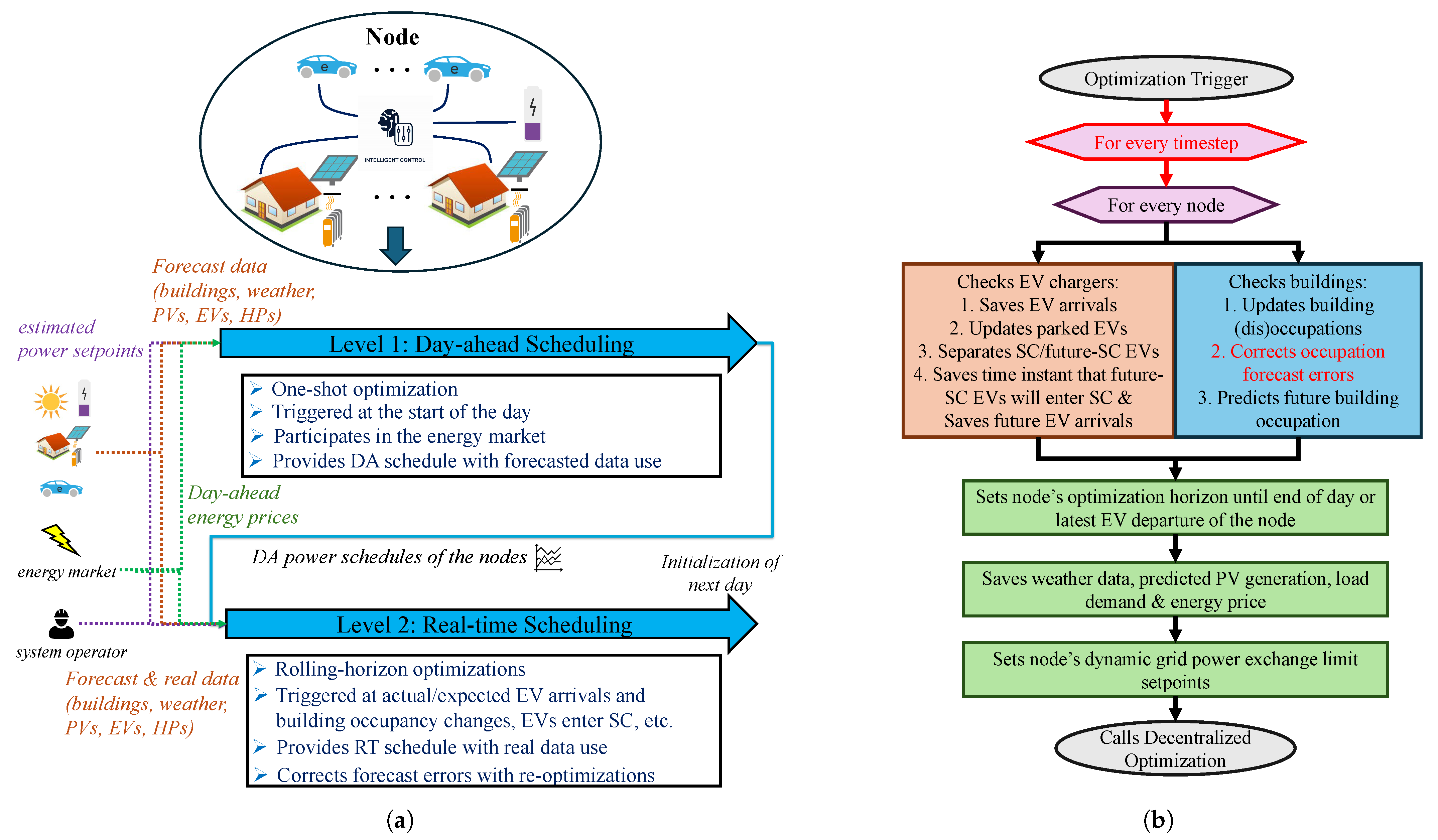
The PMS uses two optimization levels, which are described in Figure 1a. The first level is used for DA scheduling, and it is a one-shot (single) optimization of the next day. It uses forecast data about the EV driving patterns (e.g., requested energy, arrival SOC, arrival and departure time, etc.) and the buildings’ occupancy for the power management of the EVs and HPs, respectively. It is triggered at the start of the day (00:00), and in addition to providing an estimated power scheduling for the next day, it can be used in future work for other purposes, such as bidding in the wholesale reserve market for ancillary services provision. The second level is used for RT power scheduling, and it is formulated as an MPC problem that uses rolling-horizon optimization (RHO) and triggers re-optimizations upon certain events. This level initially uses predicted data about the EV driving patterns and buildings’ occupancy to manage the horizon and replaces them with actual data when the EVs finally arrive, and the buildings are (dis-)occupied, respectively.

Re-optimizations are triggered upon the events: start of the day (00:00), new/expected EV arrivals, EV participation in power management ($SOC>20\%$), and new/expected building occupancy changes. Finally, Level 2 can also be used for ancillary services provision, such as deploying offered frequency regulation reserves or congestion management. For a realistic PMS simulation, if historical data is not available for the estimated DA schedule, we assume a direct information feed between the customers and the PMS the day before. Triggering re-optimizations, the RHO of Level 2 provides uncertainty management and corrects forecast errors from the estimated DA schedule. The effectiveness of this concept has been demonstrated by inserting a level of uncertainty in all optimization triggers between the expected and the actual profiles using a normal distribution with 0′ mean and 15′ max deviation. The PMS has been successful in achieving its objectives (EV charging, building cooling/heating, PV curtailment minimization) at both levels. Hence, using a bi-level formulation can provide uncertainty management.

The flowchart of the PMS model is depicted in Figure 1b. All depicted PMS steps apply for both levels except for the red-colored ones that apply only for the RT scheduling (Level 2). Every node is checked at every timestep for optimization triggers. When an optimization is triggered, all EV chargers are checked for new EV arrivals, and the dynamic charging characteristics of every parked EV are updated. Additionally, the EVs that have $SOC>20\%$ and participate immediately in the power management (SC EVs) are separated from the EVs that will participate in the future (future-SC EVs). Thereafter, the estimated participation time of the future-SC EVs and the predicted future EV arrivals in the chargers are saved. Simultaneously, the current occupation of every building is checked, while the future dynamic building occupation is also stored. Afterward, the optimization horizon in both layers is set until the end of the day or the latest EV departure between the EVs still connected at the end of the day. The forecast data needed for the PMS, such as weather data, PV generation, load demand, energy price, etc.) during the optimization horizon is saved, and the dynamic grid power exchange limit setpoints are set for every node. All nodes share a total power capacity for grid power exchange, which is divided among the nodes according to the consumption level of their assets and is consequently used as a setpoint for imported and exported grid power. Finally, the decentralized optimization is called for the nodes with optimization triggers.

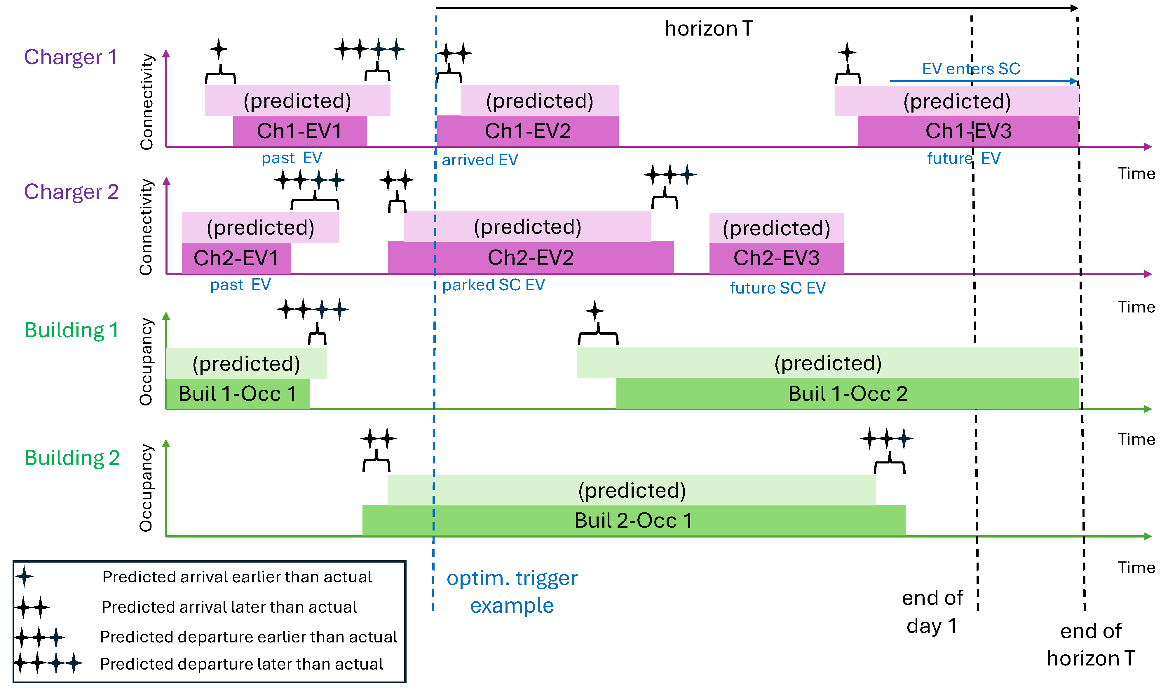
To further enlighten the function of the RHO on Level 2, an example is depicted in Figure 2. As can be seen, this node comprises 2 chargers and 2 buildings. An example of an optimization trigger is given at the actual arrival of Ch1-EV2. The PCS separates the EVs into past EVs, arrived EVs, already parked EVs, future SC EVs, and future EVs that, due to a low arrival SOC, do not enter directly into SC but after a specific time moment in the horizon. In the same manner, the buildings are separated as occupied, non-occupied, and future occupied. Because there is still a future connected EV at the end of the day, the optimization horizon is extended until its departure on the next day. For every optimization trigger, the end of the horizon still remains the same.

Regarding the correction of forecast errors in EV and arrivals/departures and buildings occupations/disoccupations, there are 4 different categories, which are marked with stars. When an EV arrives later than predicted (one star), the PMS re-optimizes at the predicted arrival moment, checks that the Ch1-EV1 has not arrived yet, and, in continuation, keeps re-optimizing for every timestep until it actually arrives. On the contrary, when an EV arrives earlier than predicted (two stars), the PMS triggers re-optimization at the arrival moment, notes that the EV arrived earlier, and does not re-optimize afterwards (until the expected/actual arrival of another EV). A similar approach applies to the departures. When the EV did not depart when predicted (three stars), the PMS keeps re-optimizing until it does, while when it departed earlier (four stars), it is erased earlier from the optimization. The corrections in the building occupancies are realized in the same manner.

4. Power Management Modeling

The developed MIQP PMS model is categorized into BESS/EV, building, node, and degradation constraints. The model constitutes an extension of the MILP problem in [66] and uses a timestep $\mathrm{\Delta }t=5^{\prime }$ to maintain an efficient trade-off between accuracy and computational expense. The utilized indices $n,j,b,bes,t,T,ch,dis,init,end$ represent the node, charger, building, BESS, time instant, optimization horizon, charging, discharging, initial, and final, respectively. All equations apply for $\forall t\in T$ unless stated otherwise.

4.1. Battery Energy Storage and EV Constraints

The EV and BESS constraints of the PMS model are listed below, where the indices $a,d$ represent the arrival and departure, respectively. The BESS modeled represents a lithium ferrophosphate battery (LFP).

$$P_{ch/dis}^{n,j/bes,t}={\mathrm{\Phi }}^{n,j}{I}_{ch/dis}^{n,j/bes,t}{V}^{n,t}$$

(1)

$$0\le P_{ch/dis}^{n,j/bes,t}\le P_{ch/di{s}_{max}}^{n,j/bes}\&0\le I_{ch/dis}^{n,j/bes,t}\le I_{ch/di{s}_{max}}^{n,j/bes}$$

(2)

Equation (1) dictates the dynamic EV and BESS charging $P_{ch}^{n,j/bes,t}$ and discharging $P_{dis}^{n,j/bes,t}$ powers, where $I_{ch}^{n,j/bes,t}$ and $I_{dis}^{n,j/bes,t}$ are the instantaneous phase charging and discharging currents, ${\mathrm{\Phi }}^{n,j}=3$ is the number of used phases, and $V^{n,t}=V_{nom}$ is the node voltage assumed steady at the nominal 230 V. The limits of charging and discharging power and current are dictated in (2), which depend on the rated LCT specifications, e.g., according to most publicly available slow AC chargers in the literature [67] or commercial V2G chargers, such as the Chademo Fermata Energy [68] (see

Table 2. BESS and EV parameters of coordinated PMS model.

Par.	Explanation	Value
$C_{e{v}_{pen}}^{n,j}$	EV Charg. Penalty	10 €/(1% SOC)
$h_{ch}^{n,j}$	EV Charg. Efficiency	0.95
$h_{bes}^n$	BESS Efficiency	0.98
$P_{c{h}_{max}}^{n,j}$	Max EV Charg. Power	$\min (P_{e{v}_r}^{n,j},22\mathrm{kW})$
$P_{di{s}_{max}}^{n,j}$	Max EV Disch. Power	$\min (P_{e{v}_r}^{n,j},20\mathrm{kW})$
$P_{ch/di{s}_{max}}^{n,bes}$	Max BESS (dis)charging Power	$0.5\mathrm{C}$
$B_{init}^{n,bes}$	BESS Initial Capacity	$0.5B_r^{n,bes}$
$V^{n,t}$	Node Voltage	230 V
${\mathrm{\Phi }}^{n,j/bes}$	Number of Phases	3
$I_{c{h}_{max}}^{n,j}$	Max EV Charg. Current	$\min (I_{e{v}_r}^{n,j},32\mathrm{A})$
$I_{di{s}_{max}}^{n,j}$	Max EV Disch. Current	$\min (I_{e{v}_r}^{n,j},29\mathrm{A})$
$S_{low}^{n,bes}$	Min BESS SOC	$10\%$
$S_{high}^{n,bes}$	Max BESS SOC	$90\%$
$V_{nom}$	Nominal Node Voltage	230 V
${\mu }_{min/max}^{bes}$	Min–Max BESS Capacity Thresholds	0.95, 1.05

).

$$B^{n,j/bes,t}=B_{init}^{n,j/bes}+\mathrm{\Delta }t{\displaystyle \sum _{t_{init}}^t}(P_{ch}^{n,j/bes,t}-P_{dis}^{n,j/bes,t})$$

(3)

$$\begin{array}{c}\hfill S^{n,j/bes,t}=B^{n,j/bes,t}/B_r^{n,j/bes}\\ \hfill S_{low}^{n,bes}\le S^{n,bes,t}\le S_{high}^{n,bes}\end{array}$$

(4)

$$I_{ch}^{n,j,t},I_{dis}^{n,j,t},B^{n,j,t}=0\forall t\notin [T_a^{n,j},T_d^{n,j}]$$

(5)

The EV/BESS battery capacity dynamics $B^{n,j/bes,t}$ at every timestep $\mathrm{\Delta }t$ are modeled in (3), where $B_{init}^{n,j/bes}$ is the initial battery capacity, equal to the arrival $B_a^{n,j}$ for EVs and 50% for the BESS. The EV/BESS SOC dynamics $S^{n,j/bes,t}$ are modeled in (4), which depend on the dynamic and rated battery capacity $B_r^{n,j/bes}$ of the BESS and EVs. The BESS SOC is always limited in a selected interval [$S_{low}^{n,bes}$, $S_{high}^{n,bes}$] to prevent accelerated aging at very low and very high SOCs. On the contrary, all variables turn to zero in (5) for the EVs outside of the EV parking time $[T_a^{n,j}$, $T_d^{n,j}]$.

$$P_{ch}^{n,j/bes,t}\le ({\displaystyle \frac{S^{n,j/bes,t}}{k}}+{\displaystyle \frac{\alpha k-\beta }{\alpha k}})P_{c{h}_{max}}^{n,j/bes}:\alpha =10,\beta =9,k=16$$

(6)

$$\begin{array}{c}\hfill I_{c{v}_{max,ch}}^{n,j/bes,t}=-\gamma I_r^{n,j/bes,t}{S}^{n,j/bes,t}+\gamma I_r^{n,j/bes,t}\\ \hfill I_{ch}^{n,j/bes,t}\le I_{c{v}_{max,ch}}^{n,j/bes,t}:\gamma =10\end{array}$$

(7)

$$\begin{array}{c}\hfill I_{c{v}_{max,dis}}^{n,j/bes,t}=\gamma I_r^{n,j/bes,t}{S}^{n,j/bes,t}\\ \hfill I_{dis}^{n,j/bes,t}\le I_{c{v}_{max,dis}}^{n,j/bes,t}:\gamma =10\end{array}$$

(8)

Equations (6)–(8) model a linear approximation of the Constant-Current–Constant-Voltage (CC-CV) BESS/EV charging/discharging region, derived by [9]. According to (6) and (7), the EVs and BESS are charged with linearly increasing power up to $SOC=90\%$, where the charging power reaches its peak value, and, consequently, the power decreases linearly to zero when SOC reaches 100%. The CV discharging region has also been considered in (8), according to which the power increases linearly to 100% when $SOC=[0\%,10\%]$, and consequently the EVs and BESS provide maximum discharging power at $SOC=[10\%,100\%]$. The variables $I_{c{v}_{max,dis}}^{n,j/bes,t},I_{c{v}_{max,ch}}^{n,j/bes,t}$ are utilized to limit the EV and BESS discharging and charging power, respectively, during their respective SOC intervals, and they depend on the rated EV and BESS currents $I_r^{n,j/bes,t}$ and the dynamic SOCs $S^{n,j/bes,t}$. Parameters $\alpha ,\beta ,\gamma ,k$ have been chosen as shown to create the slopes of the explained linear approximations but can be moderated to create steeper or flatter slopes.

$$b_{ch}^{n,j/bes,t}+b_{dis}^{n,j/bes,t}\le 1\forall t\in T$$

(9)

$$P_{ch}^{n,j/bes,t}\le b_{ch}^{n,j/bes,t}{P}_{c{h}_{max}}^{n,j/bes}\forall t\in T$$

(10)

$$P_{dis}^{n,j/bes,t}\le b_{dis}^{n,j/bes,t}{P}_{di{s}_{max}}^{n,j/bes}\forall t\in T$$

(11)

Equations (9)–(11) dictate that charging power $P_{ch}$ and discharging power $P_{dis}$ cannot be realized simultaneously. Binary variables $b_{ch}^{n,j,t}\&b_{v2g}^{n,j,t}$ are introduced and correlated to charging and discharging power, respectively, to activate only one mode at a time.

$$E_g^{n,j}=B_a^{n,j}+d^{n,j}-B_d^{n,j}$$

(12)

$$B_{end}^{n,bes}\ge {\mu }_{min}^{bes}{B}_{init}^{n,bes}\&B_{end}^{n,bes}\le {\mu }_{max}^{bes}{B}_{init}^{n,bes}$$

(13)

Moreover, (12) dictates the EV unfinished charging gap $E_g^{n,j}$, which is calculated by subtraction of the departure capacity $B_d^{n,j}$ from the sum of the arrival capacity $B_a^{n,j}$ and the requested energy $d^{n,j}$. This gap induces penalty costs for the PMS to be paid to the EV owners and is incorporated in the cost minimization of the objective function. Finally, (13) forces the final stored BESS energy $B_{end}^{n,bes}$ to remain at similar levels with the initial stored energy $B_{init}^{n,bes}$, with an accuracy error that depends on the ${\mu }_{min}^{bes},{\mu }_{max}^{bes}=5\%$ capacity thresholds, to omit the influence of the initial BESS SOC because of the daily simulation period.

4.2. Building Constraints

The constraints of the PMS model concerning the PV generation and HP heating/cooling of the buildings are listed below, derived by [4,69], where $surf,irr,sp,dhw,tank$ denote the surface, irradiation, space, domestic hot water (DHW), and tank, respectively. All constraints apply for $\forall t\in T$.

$$V_{tank}=V_{w_p}{N}_p{f}_{dhw}$$

(14)

$$A_{tank}=2\pi R_{tank}{H}_{tank}+2\pi R_{tank}^2$$

(15)

$$T_{dhw}^{n,b,t}=T_{dh{w}_{init}}^{n,b}+\mathrm{\Delta }t{\displaystyle \sum _{t_{st}}^t}{\displaystyle \frac{{(Q_{h{p}_{dhw}}-Q_{lo{s}_{dhw}})}^{n,b,t}}{V_{tank}{C}_{wat}{\rho }_{wat}}}$$

(16)

$$Q_{lo{s}_{dhw}}^{n,b,t}=U_{tank}{A}_{tank}(T_{dhw}^{n,b,t}-T_{sp}^{n,b,t})$$

(17)

$$T_{dhw}^{n,b,t_{dhw}}=T_{dhw}^{des}$$

(18)

Regarding the DHW, the total volume $V_{tank}$ and surface area $A_{tank}$ of the DHW tank are modeled in (14) and (15), where $N_p,V_{w_p},R_{tank},H_{tank}$ are the number of people in the building, the estimated water volume per person, the tank radius, and the tank height, respectively. The DHW factor $f_{dhw}$ has been set at $1.25$ to provide a 25% extra tolerance for higher DHW use. The DHW temperature dynamics $T_{dhw}^{n,b,t}$ are dictated in (16), which depend on the heating gains from the HP operation $Q_{h{p}_{dhw}}$ and heating losses $Q_{lo{s}_{dhw}}$ divided by the total thermal capacity of the tank water, where $T_{dh{w}_{init}}^{n,b}$ is the initial DHW tank temperature, $C_{wat}$ is the water specific heating capacity, and ${\rho }_{wat}$ is the water density. The tank heating losses are modeled in (17) and depend on the difference between the tank temperature $T_{dhw}^{n,b,t}$ and the building temperature $T_{sp}^{n,b,t}$, where $U_{tank}$ is the tank conductivity. Finally, (18) dictates that for every building b, the DHW tank temperature must reach the desired temperature $T_{dhw}^{des}$ at the desired time $t_{dhw}$, which has been set at 09:00 for commercial buildings and 07:00 or 19:00 for residential buildings (see

Table 3. Building parameters of the coordinated PMS model.

Par.	Explanation	Value
$C_{h{p}_{pen}}^{n,b}$	Discomfort Penalty	10 €/$\left(°\mathrm{C}\mathrm{\Delta }t\right)$
$C_{p{v}_{pen}}^{n,b}$	PV Curtail. Penalty	10 €/$\left(\mathrm{kW}\mathrm{\Delta }t\right)$
$C_b$	Build. Thermal Capacity	4.755 kWh/K
$V_b$	Build. Volume	$585{\mathrm{m}}^3$
$C_{air}$	Air Thermal Capacity	0.279 Wh/kgK
${\rho }_{air}$	Air Density	$1.225{\mathrm{kg}/\mathrm{m}}^3$
$C_{wat}$	Water Thermal Capacity	$1.16\mathrm{kWh}/\mathrm{kgK}$
${\rho }_{wat}$	Water Density	$993{\mathrm{kg}/\mathrm{m}}^3$
$r_b$	Air Change Rate	0.3 ${\mathrm{h}}^{-1}$
$T_{min}^{n,b}$	Build. Min Temp.	17°
$T_{max}^{n,b}$	Build. Max Temp.	27°
$T_{high}^{n,b}$	High Comfort Temp.	23°
$T_{low}^{n,b}$	Low Comfort Temp.	21°
$M1,M2$	Big-M Parameters	10
$T_{sup}$	HP Supply Temp.: space heating, cooling & dhw	35°, 18° & 50°
$T_{sp/dh{w}_{init}}^{n,b}$	Initial Space/DHW Temp.	22°
$T_{dhw}^{des}$	Desired DHW Temp.	50°
$N_p$	People per Build.	4
$R_{tank},H_{tank}$	Tank Radius & Height	0.23 m & 1.3 m
$V_{tank}$	Tank Volume	215 L
$U_{tank}$	Tank Conductivity	$5.98{\mathrm{W}/\mathrm{Km}}^2$
${\dot{m}}_{wat}$	HP Water Flow Rate	0.8 kg/s
$V_{w_p}$	Water Volume/Person	65 L

).

$$T_{sp}^{n,b,t}=T_{s{p}_{init}}^{n,b}+\mathrm{\Delta }t{\displaystyle \sum _{t_{st}}^t}{\displaystyle \frac{Q_{to{t}_{sp}}^{n,b,t}}{C_b+V_b{C}_{air}{\rho }_{air}}}$$

(19)

$$Q_{to{t}_{sp}}^{n,b,t}=Q_{h{p}_{sp}}^{n,b,t}{m}^{n,b}+Q_{irr}^{n,b,t}-Q_{lo{s}_{sp}}^{n,b,t}$$

(20)

$$Q_{lo{s}_{sp}}^{n,b,t}=(\sum _{sf}{U}_{sf}{A}_{sf}+C_{air}{\rho }_{air}{r}_b)(T_{sp}^{n,b,t}-T_a^t)$$

(21)

The building temperature dynamics $T_{sp}^{n,b,t}$ are modeled in (19), which depend on the initial building temperature $T_{s{b}_{init}}^{n,b}$ and the total space heating gains and losses $Q_{to{t}_{sp}}$ divided by the thermal capacity of the building mass $C_b$ and the capacity of the building air, where $V_b$, $C_{air}$, and ${\rho }_{air}$ are the building volume, the air specific capacity and air density, respectively. Equation (20) denotes that $Q_{to{t}_{sp}}$ comprise the HP heating output $Q_{h{p}_{sp}}$, the heating gains from irradiation $Q_{irr}$, and the total heating losses $Q_{lo{s}_{sp}}$, where m denotes the HP mode (+1/−1 for heating/cooling). The total heating losses $Q_{lo{s}_{sp}}$ depend on the conduction losses (first term) and ventilation losses (second term), which depend highly on the ambient temperature $T_a$ as shown in (21). The former also depends on the sum of the conductivity U over the area A of every building surface, while the latter also depends on the building air change rate $r_b$.

$$P_{h{p}_{dhw}}^{n,b,t}\le b_{dhw}{P}_{h{p}_{dhw}^{max}}^{n,b}$$

(22)

$$P_{h{p}_{sp}}^{n,b,t}\le b_{sp}{P}_{h{p}_{sp}^{max}}^{n,b}$$

(23)

$$b_{sp}+b_{dhw}\le 1$$

(24)

$$P_{h{p}_{tot}}^{n,b,t}=P_{h{p}_{sp}}^{n,b,t}+P_{h{p}_{dhw}}^{n,b,t}$$

(25)

In (22)–(24), the binary variables $b_{sp},b_{dhw}$ are introduced to enforce that the HP power consumption for DHW $P_{h{p}_{dhw}}^{n,b,t}$ and for space heating/cooling $P_{h{p}_{sp}}^{n,b,t}$ cannot occur simultaneously, where $P_{h{p}_{dhw}^{max}}^{n,b}$ and $P_{h{p}_{sp}^{max}}^{n,b}$ are the respective maximum power limits. Additionally, (25) dictates that the total HP power consumption $P_{h{p}_{tot}}^{n,b,t}$ is always the consumption for the space heating/cooling and DHW.

$$\begin{array}{c}\hfill c_{p_{hp}}^{n,b,t}=7.90471e^{-0.024(T_{ret}^{n,b,t}-T_a^t)}=7.90471e^{c_{exp}^{n,b,t}}:\\ \hfill c_{exp}^{n,b,t}=-0.024(T_{ret}^{n,b,t}-T_a^t)\end{array}$$

(26)

$$T_{ret}^{n,b,t}=T_{sup}^{sp/dhw}-Q_{h{p}_{sp/dhw}}^{n,b,t}/\left({\dot{m}}_{wat}{C}_{wat}\right)$$

(27)

Equation (26) dictates the original model of the HP’s coefficient of performance (COP) as derived by [70], which depends on the ambient temperature and the dynamic HP’s return water temperature $T_{ret}^{n,b,t}$. Due to the non-linearity of (26), the exponential part is defined as $c_{exp}^{n,b,t}$, and a piecewise linear approximation has been utilized for the COP modeling. Moreover, the HP’s return water temperature is modeled in (27), where ${\dot{m}}_{wat}$ is the flow water rate and $T_{sup}$ is the supply water temperature. $T_{sup}$ is set at 35°, 50°, and 18° for floor heating, DHW, and floor cooling, respectively, as suggested for air-to-water HPs for heating/cooling with low-temperature floor heating systems by the Sustainable Energy Authority of Ireland (SEAI) HP guide [71], and commercially available HPs, e.g., the Daikin Altherma [72].

$$\begin{array}{c}\hfill Q_{h{p}_{sp/dhw}}^{n,b,t}=P_{h{p}_{sp/dhw}}^{n,b,t}{c}_{p_{hp}}^{n,b,t}:\\ \hfill 0\le Q_{h{p}_{sp/dhw}}^{n,b,t}\le Q_{h{p}_{sp/dhw}^{max}}^{n,b}\end{array}$$

(28)

$$P_{p{v}_{dev}}^{n,b,t}=P_{p{v}_{max}}^{n,b,t}-P_{p{v}_{use}}^{n,b,t}:0\le P_{p{v}_{use}}^{n,b,t}\le P_{p{v}_{max}}^{n,b,t}$$

(29)

$$T_{dev}^{n,b,t}=\max (T_{sp}^{n,b,t}-T_{high}^{n,b},T_{low}^{n,b}-T_{sp}^{n,b,t},0):T_{min}^{n,b}\le T^{n,b,t}\le T_{max}^{n,b}$$

(30)

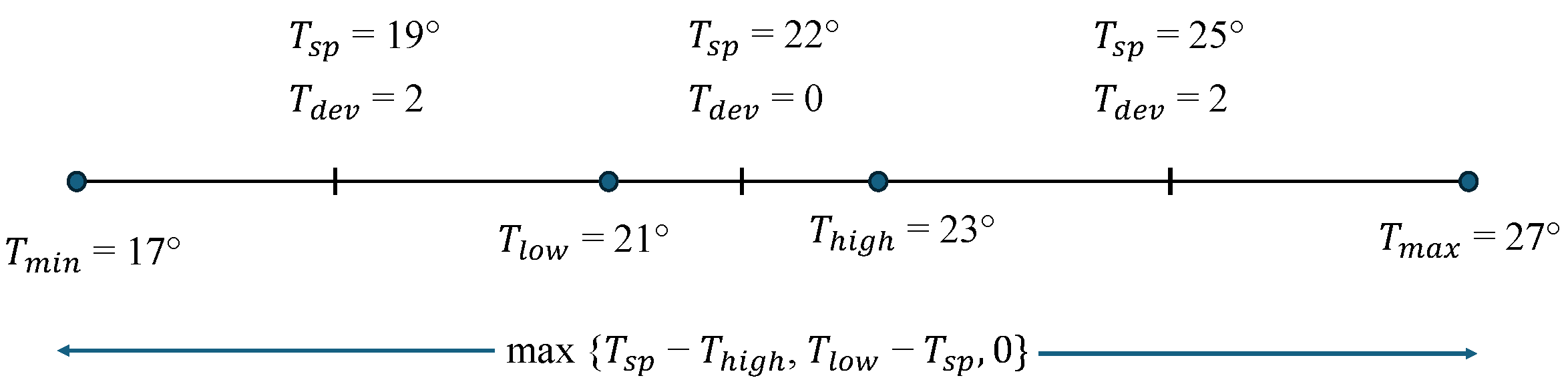
Consequently, (28) dictates the relation between the HP power consumption for space heating/cooling and DHW with the COP and their respective heating output amounts limited to the HP heating capacity $Q_{h{p}_{sp/dhw}^{max}}^{n,b}$. These equations are the only non-linear equations of the power management model that make the problem MIQP. The instantaneous PV curtailment amount $P_{p{v}_{dev}}$ is dictated in (29), where $P_{p{v}_{max}}$ and $P_{p{v}_{use}}$ are the PV generation and used PV power, respectively. The temperature deviation $T_{dev}$ is defined in (30) as the temperature difference from the nearest desired temperature interval limit $T_{low}^{n,b}$ or $T_{high}^{n,b}$. The desired temperature interval $[T_{low}^{n,b},T_{high}^{n,b}]$ has been set at [21°, 23°], while, for the needs of the model, the maximum temperature interval $[T_{min}^{n,b},T_{max}^{n,b}]$ has been set at [17°, 27°]. The variables $P_{p{v}_{dev}}$ and $T_{dev}$ are used in the objective function with cost penalties (such as with EV charging) to ensure PV max self-consumption and thermal comfort, respectively. The big-M method has been used for the linearization and integration of (30) in the PMS model, for which the reader is referred to [66]. Figure 3 depicts an intuitive explanation of (30), while Table 3 summarizes the parameters of this section.

4.3. Node Constraints

The node constraints below constitute the node power balance and the grid input and output power limits. All the node constraints apply for $\forall t\in T$.

$$P_{im}^{n,t}-P_{ex}^{n,t}={\displaystyle \sum _{j=1}^J}({\displaystyle \frac{P_{ch}^{n,j,t}}{h_{ch}^{n,j}}}-P_{dis}^{n,j,t}{h}_{ch}^{n,j})+{\displaystyle \frac{P_{ch}^{n,bes,t}}{h_{bes}^n}}-P_{dis}^{n,bes,t}{h}_{bes}^n+{\displaystyle \sum _{b=1}^B}(P_{h{p}_{tot}}^{n,b,t}+P_l^{n,b,t}-P_{pv}^{n,b,t})$$

(31)

The power balance is dictated in (31), which defines that the difference between the dynamic node imported $P_{im}^{n,t}$ and exported $P_{ex}^{n,t}$ power is the total EV/BESS charging power, HP power consumption, and base load demand cover minus the total PV rooftop generation and EV/BESS discharging power. The parameters $h_{ch}^{n,j},h_{bes}^n$ constitute the EV charger and BESS efficiencies, set at $0.95$ and $0.98$, respectively. The EV charger efficiency also comprises the EV battery losses, the BESS efficiency, and the power converter losses. The losses due to power conversion for BESS operation are lower than the respective of EV (dis)charging due to the lower needed conversion stages; power conversion for EV (dis)charging needs an additional isolation stage. Finally, (32) and (33) dictate that all the node composite power is always lower than the input and output node capacity limits, $G_{in}^n$ and $G_{out}^n$, respectively, and force the node not to import and export power simultaneously.

$$P_{im}^{n,t}={\displaystyle \sum _{j=1}^J}({\displaystyle \frac{P_{ch}^{n,j,t}}{h_{ch}^{n,j}}}-P_{dis}^{n,j,t}{h}_{ch}^{n,j})+{\displaystyle \frac{P_{ch}^{n,bes,t}}{h_{bes}^n}}-P_{dis}^{n,bes,t}{h}_{bes}^n+{\displaystyle \sum _{b=1}^B}(P_{h{p}_{tot}}^{n,b,t}+P_l^{n,b,t}-P_{pv}^{n,b,t})\le G_{in}^n$$

(32)

$$P_{ex}^{n,t}={\displaystyle \sum _{b=1}^B}(P_{pv}^{n,b,t}-P_{h{p}_{tot}}^{n,b,t}-P_l^{n,b,t})+P_{dis}^{n,bes,t}{h}_{bes}^n-{\displaystyle \frac{P_{ch}^{n,bes,t}}{h_{bes}^n}}-{\displaystyle \sum _{j=1}^J}({\displaystyle \frac{P_{ch}^{n,j,t}}{h_{ch}^{n,j}}}-P_{dis}^{n,j,t}{h}_{ch}^{n,j})\le G_{out}^n$$

(33)

4.4. Battery Degradation

Since the PMS performs energy arbitrage by using V2G and a higher number of equivalent cycles of the BESS to take advantage of the daily price deviations, it is important that the additional battery degradation cost is considered during the PMS power scheduling.

4.4.1. Non-Linear Model

$$Q_{cal}=k_{cal}(e^{-{\displaystyle \frac{E_a^c}{R}}({\displaystyle \frac{1}{T}}-{\displaystyle \frac{1}{T^r}})}{e}^{{\displaystyle \frac{\alpha F}{R}}{\displaystyle \frac{U_a^r-U_a}{T^r}}}+k_0)\sqrt{t}$$

(34)

$$Q_{cy,1}=k_{cy,1}{e}^{-{\displaystyle \frac{E_{a,cy1}}{R}}({\displaystyle \frac{1}{T}}-{\displaystyle \frac{1}{T^r}})}\sqrt{q_{tot}}$$

(35)

$$Q_{cy,2}=k_{cy,2}{e}^{-{\displaystyle \frac{E_{a,cy2}}{R}}({\displaystyle \frac{1}{T}}-{\displaystyle \frac{1}{T^r}})}{e}^{\beta {\displaystyle \frac{I_{ch}-I_{ch}^r}{c}}}\sqrt{q_{ch}}$$

(36)

The original battery degradation model dictated by (34)–(36) has been developed in [73] for an LFP cell, designed for stationary applications. More specifically, (34) models the calendar battery aging that depends mainly on the operating temperature T, SOC via the anode potential $U_a$, and time t, where $T^r$ is the rated temperature (25°) and $U_a^r$ is the anode potential at the rated SOC ($SO{C}^r=50\%$). The cyclic aging is dictated by (35) and (36), where $I_{ch/dis}^{r,cell}$ is the rated cell charging and discharging current; two equations are used for cyclic aging because different aging mechanisms are energized during charging and discharging. More in particular, (35) depends on temperature and total throughput $q_{tot}$; thus, it is activated during both charging and discharging. On the contrary, (36) depends on temperature, charging throughput $q_{ch}$, and current $I_{ch}$; thus, it is activated only during charging. All variables in (34)–(36) refer to the battery cell, while

Table 4. Battery degradation parameters of coordinated PMS model.

Par.	Explanation	Value
$k_{cal}$	Calendar coefficient in (37)	$3.694\times {10}^{-4}$
$k_0$	Constant in (37)	0.142
$k_{cy,1}$	Cyclic coefficient in (38)	$1.456\times {10}^{-4}{\mathrm{Ah}}^{-0.5}$
$k_{cy,2}$	Cyclic coefficient in (39)	$4.009\times {10}^{-4}{\mathrm{Ah}}^{-0.5}$
$\beta$	Constant in (39)	2.64 h
C	Cell capacity	3 Ah
$I_{ch}^{r,cell}$	Rated cell current	3 A
$C_Q^n$	Degradation cost	150 €/kWh
$\lambda$	Constant in (42)	${10}^{-7}$

summarizes the degradation parameters.

4.4.2. Model Linearization

The original model cannot be integrated into the MIQP problem as is because it is highly non-linear and comprises multiplication of many exponential and square-root terms. Therefore, it has been linearized by transforming it to its equivalent in the logarithmic scale.

$$\overline{Q_{cal}}({25}^{\circ },SOC=50\%)=k_{cal}(1+k_0)\sqrt{t=1day}$$

(37)

$$ln\left(Q_{cy,1}\right)=ln\left(k_{cy,1}\right)+0.5ln\left(q_{tot}^{cell}\right)$$

(38)

$$ln\left(Q_{cy,2}\right)=(ln\left(k_{cy,2}\right)-{\displaystyle \frac{\beta I_{ch}^{r,cell}}{c}})+{\displaystyle \frac{\beta }{c}}{I}_{ch}^{cell}+0.5ln\left(q_{ch}^{cell}\right)$$

(39)

Equations (37)–(39) represent the linearization of the degradation model (34)–(36). Concerning the calendar aging and (34), the duration of the simulation is fixed at one day, the BESS SOC is maintained at 50% at the beginning and end of the day, and a thermal management system is assumed to keep the operation temperature at 25°. Hence, a mean calendar capacity loss is used for the day, and (34) is transformed to (37). Moreover, assuming again a maintained temperature at 25°and using the logarithmic properties, (35) and (36) are transformed to their equivalents in the logarithmic scale (38) and (39), respectively.

4.4.3. Integration into the MIQP Model

Equation (40) correlates the EV and BESS charging and discharging currents with the cell charging and discharging currents of the respective assets $I_{ch}^{n,cell-j/bes,t}$ and $I_{dis}^{n,cell-j/bes,t}$, which are rated at $I_{ch/dis}^{r,cell}=3A$ [73]. Furthermore, the total cell current $I_{tot}^{n,cell-j/bes,t}$ is dictated in (41).

$$I_{ch/dis}^{n,cell-j/bes,t}=(I_{ch/dis}^{n,j/bes,t}/I_{max}^{n,j/bes})I_{ch/dis}^{r,cell}\forall t\in T$$

(40)

$$I_{tot}^{n,cell-j/bes,t}=I_{ch}^{n,cell-j/bes,t}+I_{dis}^{n,cell-j/bes,t}\forall t\in T$$

(41)

Moreover, (42) models the EV and BESS total and charging cell throughput dynamics $q_{tot,ch}^{n,cell-j/bes,t}$, which are needed for the calculation of $ln{\left(q_{tot,ch}\right)}^{cell-j/bes}$ in (38) and (39) with the use of the parameter $\lambda ={10}^{-7}$ to avoid infinity at zero current. Additionally, (43) dictates the limits of the cell total and charging current and throughput.

$$q_{ch/tot}^{n,cell-j/bes,t}=I_{ch/tot}^{n,cell-j/bes,t}\mathrm{\Delta }t+\lambda \forall t\in T$$

(42)

$$\begin{array}{c}\hfill 0\le I_{ch}^{n,cell-j/bes,t},I_{tot}^{n,cell-j/bes,t}\le 3\forall n,t\in T\\ \hfill 0\le q_{ch}^{n,cell-j/bes,t},q_{tot}^{n,cell-j/bes,t}=3\mathrm{\Delta }t\forall n,t\in T\end{array}$$

(43)

The variables $q_{ch}$ and $q_{tot}$ are transformed to their equivalent $ln\left(q_{ch}\right)$ and $ln\left(q_{tot}\right)$, respectively, using linear piecewise approximations of the function $y=ln\left(x\right)$, while $ln\left(Q_{cy,1}\right)$ and $ln\left(Q_{cy,2}\right)$ are similarly transformed to their equivalent $Q_{cy,1}$ and $Q_{cy,2}$, using the function $x=e^y$. The resulting degradation variables $Q_{cal}$, $Q_{cy,1}$, and $Q_{cy,2}$ constitute capacity loss percentages. In this regard, (44) represents the degradation objective, which minimizes the total BESS/EV cyclic aging with the addition of the mean BESS/EVs’ calendar aging $\overline{Q_{cal}}$. Finally, the total BESS/EV battery aging is calculated post-optimization with the original model (34)–(36) for verification purposes.

$$\begin{array}{c}\hfill \min B_{Qtot}^n=\min \mathrm{\Delta }t({\displaystyle \sum _{t=1}^T}(Q_{cy,1}^{n,bes,t}+Q_{cy,2}^{n,bes,t})B_r^{n,bes}+\\ \hfill {\displaystyle \sum _{j=1}^J}(Q_{cy,1}^{n,j,t}+Q_{cy,2}^{n,j,t})B_r^{n,j})+\overline{Q_{cal}^{n,bes}}{B}_r^{n,bes}+{\displaystyle \sum _{j=1}^J}\overline{Q_{cal}^{n,j}}{B}_r^{n,j}\end{array}$$

(44)

The utilized empirical degradation model considers various degradation factors such as temperature, time, C-rate, and throughput. However, it fails to consider the effects of SOC and depth of discharge (DOD), especially for the cyclic aging. Therefore, there is an accuracy loss for cycling during very high SOCs and DODs. Therefore, the following measures have been considered:

(1) Stationary BESS: The SOC is directly limited to deviate within the interval [10%, 90%] so that the battery is never completely depleted or charged.

(2) EVs: Firstly, the EVs are allowed to participate in the power management only after their SOC reaches 20%. Secondly, due to the CC-CV region, the EVs actively perform energy arbitrage when they are being charged in the CC region. When $SOC>90\%$, the EVs stop being consecutively charged and discharged due to the low power levels and afterwards are charged uncontrollably until departure.

4.5. Objective Function

Finally, the PMS objective function for every node n is dictated in (45). The PMS is a multi-objective MIQP model that has translated all objectives into a total cost aimed to be minimized. In this regard, all penalty costs are chosen to be much higher than the energy price to attach great importance to the customers’ comfort (see Table 2 and Table 3). The total cost comprises:

(a) For energy arbitrage: The minimum exchange grid power cost, where $P_{im},C_{buy}$ and $P_{ex},C_{sell}$ are the imported and exported power and related costs.

(b) For PV max self-consumption: The total PV curtailment cost, where $C_{p{v}_{pen}}$ is the related penalty.

(c) For thermal comfort maintenance: The total thermal discomfort cost, where $C_{h{p}_{pen}}$ is the related penalty and $O^{t,n,b}\in [0,1]$ is the dynamic building occupancy.

(d) For charging comfort maintenance: The total EV unfinished charging cost, where $C_{p{v}_{pen}}$ is the related penalty.

(e) For battery degradation mitigation: The total battery degradation cost, where $C_Q^n$ is the degradation cost. The placement of (44) inside (45) directly mitigates battery degradation. In this work, the weights of the different objectives have been adjusted in association with the respective costs. However, placing a higher weight would give a higher importance to battery degradation minimization and, hence, directly decrease it through the objective function.

To further analyze the cost objective function, this PMS represents a multi-objective problem which aims to co-optimize simultaneously various different objectives: PV curtailment, charging and thermal comfort, cost savings, and battery degradation. Translating every objective into cost, the multi-objective problem becomes single-objective with the goal of minimizing the overall cost. In that way, the cost of every objective becomes the respective weight in the overall cost function. The energy and battery degradation prices were selected to accurately represent the conditions of the PMS. The energy price $C_{buy}$ deviates between 0.20 and 0.24 €/kWh, as derived for the year 2021 by [74]. Moreover, the degradation cost $C_Q^n$ was set constant at 150€/kWh for every lost kWh, as derived by [75].

Finally, all the used penalties for EV charging, thermal discomfort, and PV curtailment were chosen intuitively to be well above the typical energy cost per kWh in the Netherlands, ×10 times over. The reasoning behind this choice is that the PMS does not prioritize the cost savings over the cover of the customers’ needs. For example, if the cost penalty for EV charging comfort were comparable to the energy prices, the PMS would try to make a decision about charging an EV at favorable prices or not charge the EV at all. However, for the PMS we aimed to develop, it has no value to perform energy arbitrage if the EVs are not charged or the buildings are not heated at the required level expected by the customers.

$$\min C_n=\mathrm{\Delta }t\left({\displaystyle \sum _{t=1}^T}(P_{im}^{n,t}{C}_{buy}^t-P_{ex}^{n,t}{C}_{sell}^t)\right)+{\displaystyle \sum _{t=1}^T}{\displaystyle \sum _{b=1}^B}\left(P_{p{v}_{dev}}^{n,b,t}{C}_{p{v}_{pen}}^{n,b}\right)+{\displaystyle \sum _{t=1}^T}{\displaystyle \sum _{b=1}^B}\left(T_{dev}^{n,b,t}{C}_{h{p}_{pen}}^{n,b}{O}^{t,n,b}\right)+{\displaystyle \sum _{j=1}^J}{E}_g^{n,j}{C}_{e{v}_{pen}}^{n,j}+B_{Qtot}^n{C}_Q^n$$

(45)

All PMS parameters used in Section 4 for the modeling of EV/BESS, buildings, and battery degradation are summarized in Table 2, Table 3, and Table 4, respectively. For the detailed explanation of the parameters used in Table 2 and Table 3, as well as for the described EV charging and building heating models, the reader is referred to our previous works in [4,69], on which this work is based. To give a small summary, as already mentioned, the 95% EV charging efficiency and maximum charging power/current levels are based on publicly available slow AC chargers in the literature [67] and commercial V2G chargers [68]. The higher 98% BESS one-way charging efficiency was selected because BESS charging requires fewer conversion stages than EV charging (no need for galvanic isolation) and is consistent with BESS efficiency studies in the literature, such as [76]. The BESS SOC and C-rate limits were used to further limit the battery degradation.

Moreover, regarding Table 3, the building’s thermal capacity and volume were chosen to represent the building as a first-order lumped RC thermal model based on EN ISO 13790. The effective thermal capacitance was selected to represent the active thermal mass of the residential building and is consistent with values commonly adopted in reduced-order building thermal models, which use the ISO 13790 5R1C methodology [77]. The values of air/water specific capacity and density are well established in the literature, while the building’s 0.3 h⁻¹ air change rate is extensively used in buildings, such as in [78]. The HP specifications (e.g., supply temperature, water flow rate, etc.) are derived from the SEAI HP guide [71] and commercially available HPs [72], while the tank specifications (dimensions, conductivity, etc.) are based on both commercial HP tanks [79] and standard tank energy losses assessment approaches [80]. Additionally, all BESS degradation parameters in Table 4 are derived from the work of the original non-linear battery cell degradation model [73].

5. Case Studies and Scenarios

5.1. Small and Large Load-Scale Scenarios

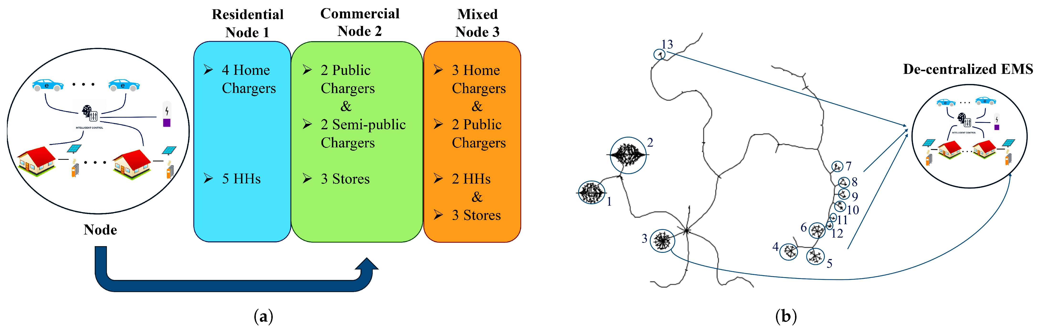
Two load-scale scenarios have been used for the testing of the PMS. The small load scenario consists of three nodes from different areas (residential, commercial, and mixed). It has been assumed that the three nodes are connected with different radial feeders to the main grid. Each node comprises a 50 kWh-rated BESS unit of 0.5 C max C-rate, while Figure 4a depicts the number of buildings and chargers per node. Buildings in residential areas, e.g., households (HHs), are occupied longer during the day (00:00–08:00, 14:00–00:00) compared to commercial buildings such as offices and stores that are mostly occupied during the day (09:00–21:00). Moreover, home chargers at residential areas are characterized by a lower frequency of incoming EV fleets which remain parked for longer times and arrive with lower SOCs compared to public and semi-public chargers. Furthermore, EVs consume approximately a 30% higher amount of energy due to cabin heating [4] during winter, while building heating consumes 50% higher amount of energy than building cooling during summer because of a higher temperature difference with ambient temperature (hence, lower COPs) [69]. Finally, the input and output node capacity limits, $G_{in}^n$ and $G_{out}^n$, respectively, are set at 400kW.

The large load scenario is depicted in Figure 4b and is a real urban grid in the Netherlands. Each one of the 13 load locations, hereby called nodes, comprises several loads (buildings) equipped with PVs, HPs, and EV chargers.

Table 5. Node characteristics of large load scenario (adapted from [81] (CC BY)).

Nodes	Buildings (PVs, HPs)	Chargers	BESS Capacity [kWh]
1	32	32	320
2	44	44	440
3	18	18	180
4	6	6	60
5	6	6	60
6	6	6	60
7	2	2	20
8	2	2	20
9	2	2	20
10	2	2	20
11	1	1	10
12	1	1	10
13	1	1	10

summarizes the number of LCTs at every node. Moreover, a BESS is installed at every node, whose capacity is set at 10 kWh per building/charger. Finally, the input and output node capacity limits, $G_{in}^n$ and $G_{out}^n$, respectively, are set at 3.785 MW for the large load example.

5.2. Data Input

The following data is used as input in the PMS:

(1) Dutch residential and commercial electricity distribution consumption profiles (year 2022) have been acquired from [82].

(2) Probability distribution functions (PDFs) of EV driving patterns, such as arrival and departure times, arrival SOCs, and requested energy by the Elaad EV charging open database [83].

(3) Weather data, such as ambient temperature, incident irradiation, wind speed, etc., which has been used for the creation of the PV generation profiles and the heating losses calculation by the Meteonorm database [84].

(4) Day-ahead market (DAM) energy price profiles (year 2022) have been acquired by the Dutch ENTSO-E platform [74].

(5) The LV distribution grid used in the large load scenario was acquired by the Dutch distribution system operator (DSO) Enexis Groep, and it represents a real Dutch distribution grid [85].

(6) A 3 kW-rated reversible HP module [72] and a 3 kW-rated HIT N245 PV module [86] for the building heating and PV generation, respectively. Moreover, the EV pool comprises the 11 kW-rated “Hyundai Kona, BMW I3, Jaguar I-Pace, and Tesla Model 3”, the 16 kW-rated “Tesla Model X and Tesla Model S”, and the 22 kW-rated “Renault Zoe” EVs.

(7) The Sony US26650FTC1 LIB iron phosphate/graphite cell of 3.2 V and 3 Ah nominal voltage and capacity, designed for stationary applications, derived by [73].

(8) Finally, the detailed version of the PV model that uses the weather data and the PV module specifications to extract the PV generation data can be found in [4]. Moreover, the respective detailed version of the HP model, which also describes the building modeling and the occupancy profiles, can be found in [69].

The input data (1)–(8) together with their sources and their explanation uses are summarized in

Table 6. Summary of data input sources, explanation, and utilization.

Source	Explanation	Utilization
[82]	Electricity distribution consumption profiles	Base load modeling
[83]	PDFs of EV driving patterns	EV fleets modeling (parking times, arrival SOC, requested energy, etc.)
[84]	Weather data	PV generation and heating losses
[74]	DAM energy price profiles	Objective function
[85]	LV distribution grid	Large-scale load scenario
[72]	HP module	HP consumption modeling
[86]	PV module	PV generation modeling
[73]	BESS module	BESS and degradation modeling
[69]	HP and building models	HP consumption modeling
[4]	PV models	PV generation modeling

.

To incorporate a level of uncertainty, Monte-Carlo Simulation has been used to generate (a) 600 random EV fleet profiles for Home, Semi-public, and Public chargers from the PDFs of (2), (b) 200 residential and commercial building occupancy profiles with random occupancy changes, as discussed in Section 3, and (c) 180 Summer and Winter PV generation profiles with random PV module orientations using the data of (3) and PV modeling in [69]. Afterward, LCT profiles have been randomly selected and distributed in the utilized load scenarios. It must be noted that this work has not developed specific forecast models for the acquired input data, hence the base load and energy prices profiles and weather data. Only specific PV and HP modules and a small pool of EVs were considered. As explained, using the stochastic EV arrival/departure data from Elaad and PV orientations (tilt angle in [0°, 90°] and azimuth in [0°, 180°]), a number of random EV consumption and PV profiles were created. Moreover, using an accuracy error of [0′, 15′], a number of deviated EV profiles and building occupancy profiles were created, the latter of which have a direct impact on the HPs. These profiles were fed to both optimization levels, except for the deviated profiles, which were fed only to Level 2. These deviated profiles were used to test the functionality of the RHO on correcting forecast errors, and this is a first step of uncertainty management. However, the RHO can be enhanced in a similar manner to correct forecast errors in all other types of data input or can be combined with stochastic or robust optimization, as also written later in our limitations and future work.

5.3. Overall Case Studies

Table 7. Case studies and scenarios of the PMS.

Cases	Flexibility	Season	Scenario	Degr.	Time
1	Loads	Winter	Small Load	No	38′
2	Loads	Summer	Small Load	No	37′
3	Loads & BESS	Winter	Small Load	No	41′
4	Loads & BESS	Summer	Small Load	No	41′
5	Loads & BESS	Winter	Small Load	Yes	1 h & 2′
6	Loads & BESS	Summer	Small Load	Yes	59′
7	Loads	Winter	Large Load	No	7 h & 50′
8	Loads	Summer	Large Load	No	7 h & 45′
9	Loads & BESS	Winter	Large Load	No	8 h & 5′
10	Loads & BESS	Summer	Large Load	No	7 h & 55′
11	Loads & BESS	Winter	Large Load	Yes	10 h & 3′
12	Loads & BESS	Summer	Large Load	Yes	9 h & 57′

summarizes the case studies of this work with their respective simulation times. Cases 1–6 are devoted to the small load scenario, and cases 7–12 to the large load scenario. Cases 1, 3, and 5 investigate the power management of flexible loads, flexible loads + BESS, and flexible loads + BESS + degradation for winter, while cases 2, 4, and 6 investigate the related comparisons during summer. Accordingly, the same applies to the large load scenario in cases 7–12. Overall, the case studies described above aim to quantify and reflect on the effect of the following influencing factors on power management characteristics (cost, grid power exchange amount, V2G energy use, BESS energy use, power flows scheduling, etc):

(1) Flexibility of loads and BESS: Stationary BESS and flexible loads, such as EVs and HPs, can both offer flexibility for energy arbitrage. While the BESS is expected to be capable of the highest flexibility because it is not prone to uncertainties, the contribution of flexible loads can be proven comparable in large aggregated loads.

(2) Load-size and load-type effect: Different load types, such as residential and commercial, can highly influence the PMS decision-making due to different characteristics of buildings and EV fleets. Additionally, a larger load scale that comprises a higher number of present flexible loads can be proven to be more flexible, also without the use of a BESS.

(3) Seasonal effect: Different seasons can have a significant impact on the consumption and power levels of the flexible loads as well as on the PV generation. Thus, it is important to encapsulate the yearly seasonal variations in the investigation of the PMS performance.

(4) Battery degradation effect: Constant battery charging and discharging can highly increase the steepness of the capacity fading and induce further costs. Therefore, especially in large load scales, accumulated degradation costs can become significant and alter the energy arbitrage decision-making.

5.4. Accuracy and Computational Burden of MIQP Formulation and Battery Degradation Model

As expected, MIQP problems are most often computationally heavier than the MILP problems, even if they do not have non-convex constraints or objective functions. In this work, the consideration of a variable HP COP in (28) made the model MIQP. Other existing PMS studies with HPs assumed a steady COP, e.g., [36,52], to keep their formulation as MILP, accepting a loss of accuracy. Moreover, the integration of the degradation model in cases 5, 6, 11, and 12 does not jeopardize the solvability of the PMS, because the constraints it adds to the PMS are linear and do not affect the convergence. However, it increases the computational time considerably. As Table 7 summarizes, regarding cases 1–6 of the small-scale load scenario, BESS integration in cases 3–4 increased the time by 3′ compared to the 38′ of cases 1–2 (7.9%). However, BESS degradation increased the time by approximately 20 min; hence, up to a 50% increase. Moreover, observing cases 7–12 of the large-scale scenario, BESS degradation in cases 11–12 added another 2 h to the 8 h needed in cases 9–10; hence, a 25% increase. After the simulation of the cases, the average COPs were calculated to be 3.4 and 6 for winter and summer, respectively. By omitting (26) and (27), (28) becomes linear and the model becomes MILP. Cases 1–6 were re-simulated with the MILP formulation, and the simulation time and optimal cost accuracy error were calculated. The accuracy error reached up to 6% for summer in cases 2, 4, and 6, while it reached up to 10% for the winter in cases 1, 3, and 5. On the contrary, the simulation time decreased up to 10% and 20% for cases 1–4 and cases 5–6, respectively.

Due to the convex nature of the problem, the solvability of the problem is not affected, and it does not lead to convergence errors in any case study. However, it can be seen that the combination of MIQP approach and battery degradation integration is computationally heavy for the PMS and considerably increases the computational time, especially for the large-scale load scenario. For example, while in the small load scenario, it can reach up to 1 h of simulation, while this time response reaches approximately 10 h for grid-level aggregator loads. To further explain the size of the optimization problem during the considered case studies,

Table 8. Size of optimization problem per case study.

Cases	LCTs	Nodes (Parallel Optim/s)	Continuous Variables	Binary Variables	Constraints	PWL Segments
1	39	3	383	52	620	26
2	39	3	383	52	620	26
3	42	3	410	58	686	32
4	42	3	410	58	686	32
5	42	3	538	58	894	64
6	42	3	538	58	894	64
7	369	13	3593	492	5820	246
8	369	13	3593	492	5820	246
9	382	13	3710	518	6106	272
10	382	13	3710	518	6106	272
11	382	13	4798	518	7874	544
12	382	13	4798	518	7874	544

summarizes the LCTs, number of nodes (which represent the in-parallel optimizations), the continuous and binary variables, the constraints, and the piecewise-linear segments in every case study. It can be seen that for cases 11 and 12 of the large load scenario, which are the cases that comprise all the considered features, the constraints and continuous variables reach up to 7874 and 4798, respectively. Moreover, the binary variables and PWL segments, which are the aspects that considerably slow down the optimization, reach up to 518 and 544 for cases 11 and 12, respectively, compared to the respective 58 and 64 of cases 5 and 6 of the small-scale scenario. Moreover, Table 8 shows the characteristics of the day-ahead optimization of Level 1, while Level 2 can comprise up to approximately 50 more re-optimizations during the daily optimization horizon. Thus, it can be seen why cases 11 and 12 of the large load scenario can reach up to a 10 h runtime.

Hence, according to the authors’ knowledge, it can be concluded that the developed PMS serves well for day-ahead and real-time scheduling for systems of small or moderate size, such as an aggregation of buildings and EV chargers within a district, while it is more suitable for planning purposes for aggregations of grid-level loads. In future work, it can be investigated if reducing the computational expense by transforming the problem into MILP and simultaneously reducing the number of binary variables and PWL segments of the optimization could make the PMS suitable also for real-time operation of grid-level load aggregation.

5.5. Simulation Setup and Utilized Software

The simulation timestep has been set to 5 min to show in detail the power flow decision-making of the PMS with a reasonable computational time. Moreover, the simulation duration was set to 1 day for both winter and summer seasons. Concerning the utilized software, the model was developed in a Python 3.9 environment and was solved with the Gurobi 11 solver due to its powerful capabilities in solving MIP problems. Finally, the simulations were performed with an Intel (R) 11th Gen Core(TM) i7-3.00 GHz processor with 16 GB installed RAM.

5.6. Limitations

The main limitations of this work are as follows: Firstly, the uncertainties considered are the building occupation and the EV driving patterns. However, there are multiple other uncertainties in the PMS, such as PV generation, load demand, etc., which should also be managed on Level 2 using the re-optimization of RHO. Moreover, instead of assuming a perfect forecast of weather data, energy prices, load demand, etc., effective forecast models should be applied and evaluated to increase the uncertainty consideration of the work. The RHO of Level 2 should also be enhanced with stochastic or robust optimization to increase the related uncertainty management.

Secondly, daily simulations were performed due to computational time. The selection of a weekly simulation, which would be the closest to the average of the season, would provide more insights, such as intra-week effects. Thirdly, modeling non-linearities (e.g., CC-CV, COPs) has been integrated with piecewise linear functions in the MIQP problem, while charging efficiencies, which are power-dependent, have been considered steady. Their consideration of the use of a non-linear solver is proposed for future work to address the level of accuracy decrease. Moreover, while the empirical battery degradation model accounts for most degradation mechanisms (time, C-rate, temperature, throughput, etc.), it does not consider the effects of high SOC and DOD on cyclic aging.

Finally, the scalability and performance of the model have only been evaluated regarding the increasing scale of the loads and not of the grids themselves. Hence, the grid topologies have been ignored together with important aspects such as the nodal optimal power flows and the consideration of the power losses, voltage deviations, and interactions between the nodes, which are also proposed for future work. However, the insights of our work, such as comparison of V2G and BESS use, total cost, and incurred degradation, etc., depend highly on the load scale, and the proposed large load-scale scenario comprises hundreds of buildings and EV chargers; thus, according to the authors’ point of view, it can support the claiming of this work.

6. Results

The results of the two load scenarios for Level 1 are presented below. Apart from some numerical differences due to the forecast error corrections, the insights of the work remain similar for Level 2.

6.1. Small Load Scenario

6.1.1. Power Management Without BESS

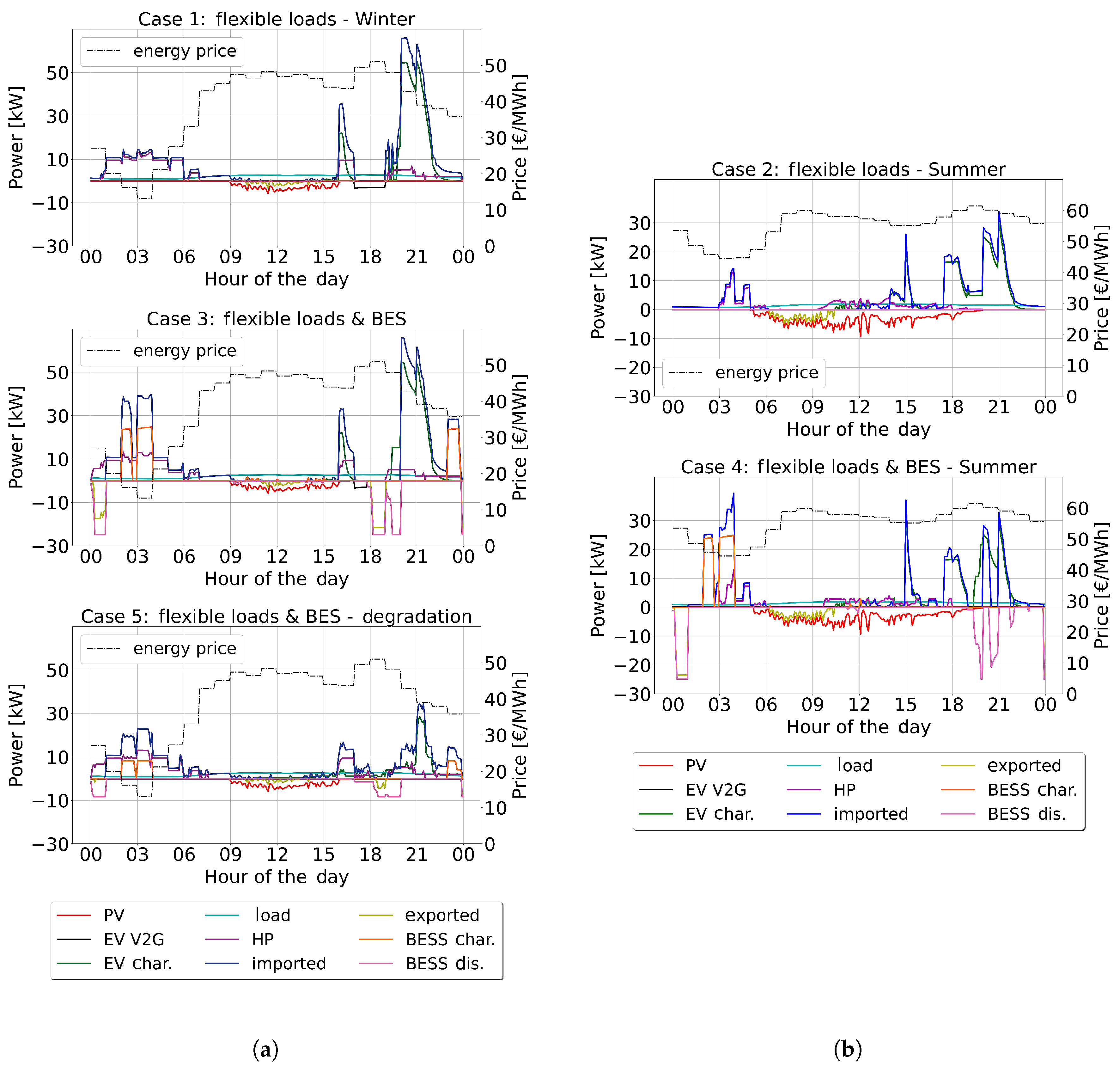
The power flows of Node 3 for winter cases 1,3, 5 and summer cases 2, 4 are depicted with the daily energy prices in Figure 5a and Figure 5b, respectively. In Case 1 (Figure 5a), grid power is imported during low energy prices [00:00–07:00] for building and DHW heating, while during [07:00–09:00], power is imported only for base load cover. Moreover, the highest energy price peak during [17:00–19:00] is avoided, and EVs are charged during the periods [16:00–17:00] and [19:00–00:00]. Additionally, V2G energy is utilized during the highest price peak to cover the base load demand. Finally, PV generation covers the load and is mostly exported because it coincides with the high energy prices [09:00–16:00]. On the contrary, in Case 2 (Figure 5b), the higher and prolonged summer PV generation is initially exported during the increasing energy prices of [05:00–10:00] and is consequently used until 19:00 for EV charging, load cover, building cooling, etc. Similarly, the high energy price peak of [19:00–20:00] is mostly avoided, while V2G energy is not preferred due to the availability of PV generation, which causes lower power losses.

6.1.2. Power Management with BESS

In Figure 5a, PV generation use, EV charging, and HP operation remain similar for cases 1 and 3. BESS is mostly charged with grid power during the lowest energy prices of [02:00–04:00], is discharged back to the grid during the highest prices of [18:00–19:00], while it is also used for EV charging and base load cover during [19:00–20:00]. Additionally, the V2G energy use during the high energy prices is considerably decreased compared to Case 1, and BESS use is preferred due to the lower power losses. Similarly, in cases 2 and 4 of Figure 5b, the management of PV generation and flexible loads behaves the same as in cases 1 and 3. However, while BESS is mainly charged again during the low prices of [02:00, 04:00], it is discharged for EV charging during the high energy prices of [19:00, 21:00]. Hence, BESS is used more for the flexibility of the node in Case 4, because most revenues are ensured by the PV generation. On the contrary, BESS is used in Case 3 mostly for revenues and cost compensation to compensate for the high imported grid energy due to the low PV availability.

6.1.3. Power Management with Battery Degradation

Regarding Case 5 in Figure 5a, the BESS charging and discharging periods remain similar with and without consideration of battery degradation cost; however, the power levels are notably decreased. Moreover, the discharged BESS energy is more utilized for building heating and EV charging than for power exportation to the grid for revenues. Hence, the BESS use is highly decreased and is preferred only for the basic needs of the node (EV charging and building heating without penalty costs) during the high energy price peaks of [17:00, 20:00]. Additionally, V2G energy is not used due to the combined high round-trip power losses and additional degradation costs. Finally,

Table 9. BESS Capacity Fading for Nodes 1–3: Cases 3–5 and Cases 4–6.

	Case 3		Case 5		Case 4		Case 6
Nodes	Daily (Wh)	Yearly (%)	Daily (Wh)	Yearly (%)	Daily (Wh)	Yearly (%)	Daily (Wh)	Yearly (%)
Node 1	3.49	2.54	2.35	1.72	2.88	2.1	1.71	1.24
Node 2	3.66	2.68	2.47	1.8	2.72	1.98	1.34	0.98
Node 3	3.41	2.48	2.4	1.76	2.29	1.76	1.16	0.84

summarizes the daily capacity fading in (Wh) and the yearly extrapolation in (%) for the BESS for all nodes and cases 3–6, showing the effectiveness of the degradation optimization model. For example, while BESS capacity fading is approximately 2.5% in Case 3, it drops to 1.8% in Case 5.

6.1.4. Power Management Cost and Grid Power Exchange Summary

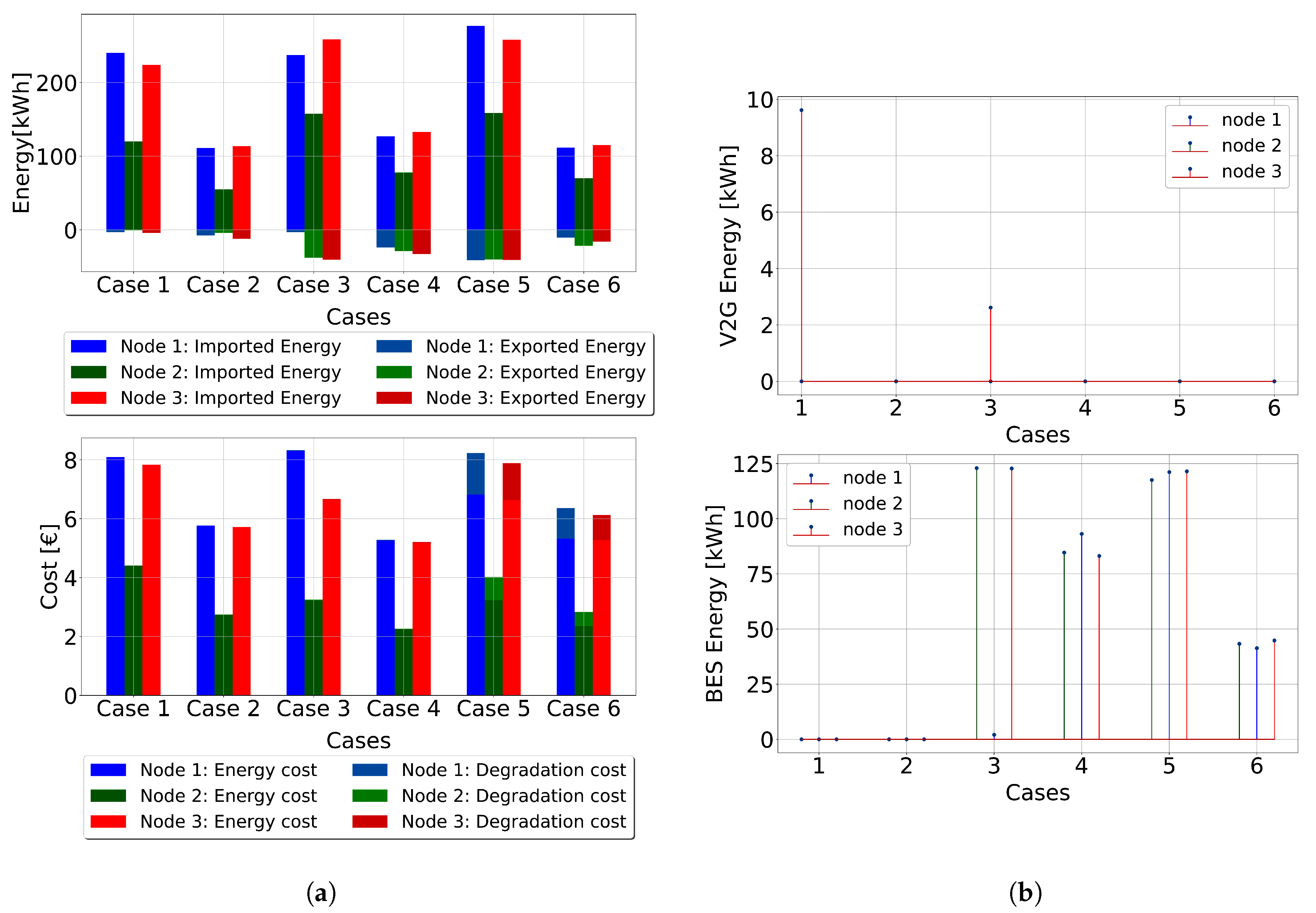
Figure 6a depicts in the upper plot the total imported and exported energy and in the lower plot the total cost (energy cost and degradation cost) of the 3 nodes. Winter cases 1, 3, and 5 have always had higher costs than their respective summer cases 2, 4, and 6 (up to 60%) because of the higher amount of imported power, as discussed in Section 5. For example, Node 1 imported 240 kWh and 110 kWh in cases 1 and 2, respectively, (118% increase). Moreover, using a higher PV generation in summer reduces the total cost, either with direct use or with grid exportation for revenues. Overall, cases 1–2 export the least amount of energy for all nodes since they are the least flexible (no BESS). Furthermore, BESS use addition decreases the cost for most nodes by a factor up to 16% (Node 3 in Case 3 compared to Case 1), while the amounts of imported and exported grid power are also increased for all nodes when cases 3 and 4 are compared to cases 1 and 2, respectively. Additionally, in battery degradation cases 5 and 6, the total cost always increases for all nodes when comparing them with their respective cases 3 and 4. While the energy cost can be lower (e.g., Node 1 in Case 5 compared to Case 3) due to lower grid power exchange to avoid higher degradation, when the degradation cost is summed up, the total cost results are always equal to or higher.

The node type also strongly impacts the exchanged grid power and total cost. The commercial node (Node 2) is generally characterized by a lower cost in all cases. This is because, as explained, commercial buildings (e.g., stores and offices) are occupied less during the day than residential buildings, and EVs are parked for a lower parking time in public chargers and request a lower amount of energy. Hence, the needed imported grid power is considerably lower (by approximately 50%) for the commercial node. For that reason, there is also a larger power window in the feeder to export BESS energy and PV generation for revenues, and, hence, Node 2 exports considerably more power when BESS is introduced, almost comparable to Node 3, which is the most flexible node. Hence, highly flexible nodes or nodes that occupy less of the power capacity can use their BESS capacity more for revenues. Finally, the degradation cost is always higher for nodes 1 and 3 because they comprise home chargers where EVs arrive with a lower SOC and request higher amounts of energy.

6.1.5. BESS Energy and V2G Energy Use Summary

Regarding the use of BESS and V2G, Figure 6b depicts the total V2G energy used (upper plot) and the total BESS energy used (lower plot) per node and case. V2G is used only in winter cases 1 and 3, because PV generation is available for a shorter time. For example, V2G energy is generally used during high energy price peaks. During the winter price peaks of [17:00–20:00], there is no more available PV generation. Moreover, concerning all other cases, BESS use is always preferred over V2G due to the higher BESS efficiency and lower power losses. The influence of seasonal variations of PV generation on V2G energy use has also been seen in [66]. In cases 5 and 6, where there is additional degradation cost combined with the power losses, V2G energy use becomes inefficient even during winter. Finally, V2G energy is more likely to be used in Node 3 (the mixed node), which has the highest flexibility, comprising both residential and commercial buildings and home and (semi-)public chargers. Regarding BESS energy use, as already discussed, winter (cases 3 and 5) favors using BESS for charging and discharging power to the grid for revenues for most of the nodes. On the contrary, the available PV generation is preferred during summer for power exportation, and the BESS is mostly used for the needs of the node instead. Finally, the consideration of battery degradation decreases the use of BESS, especially during summer, due to the additional degradation cost.

6.2. Large Load Scenario

6.2.1. Flexible Loads and BESS

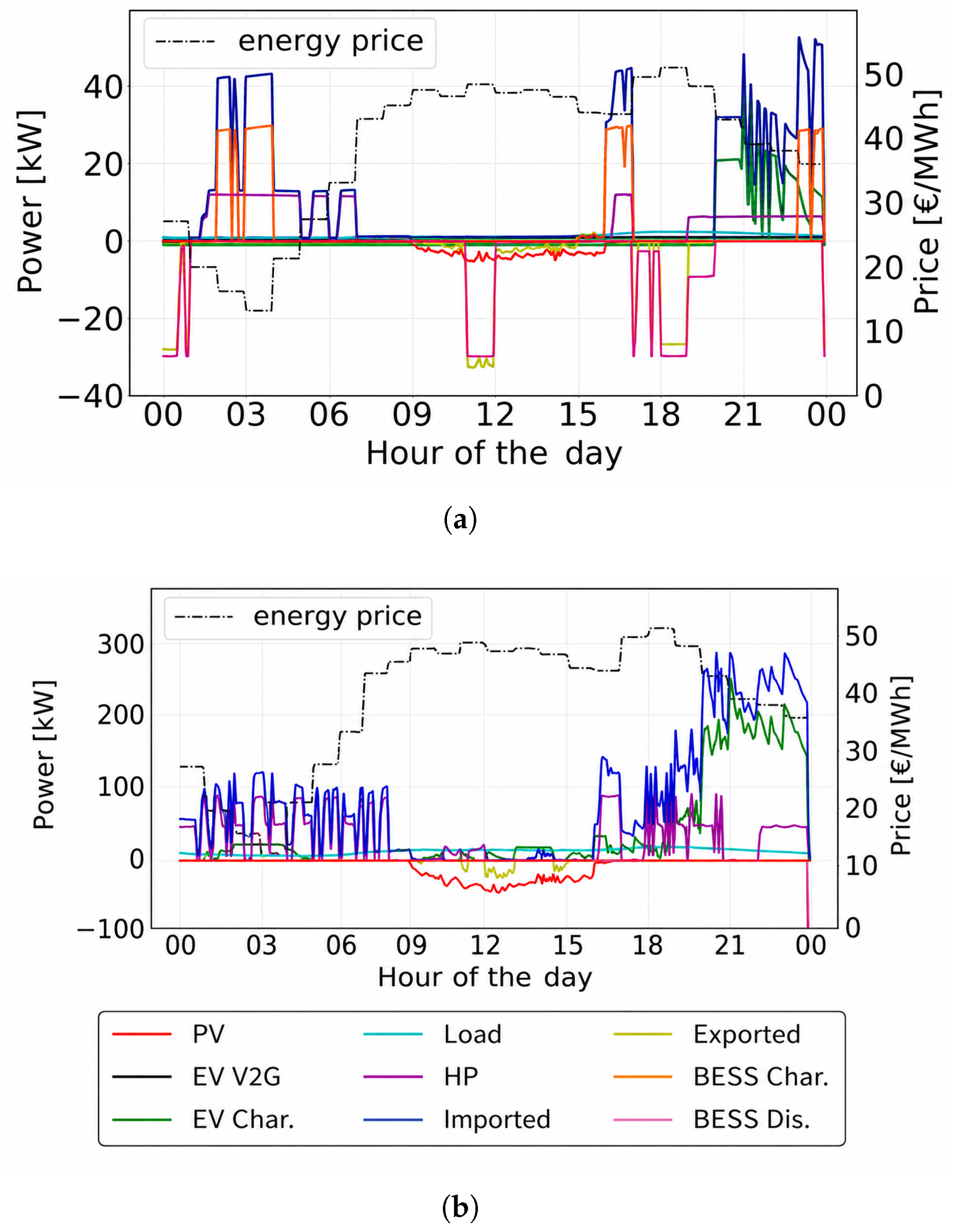
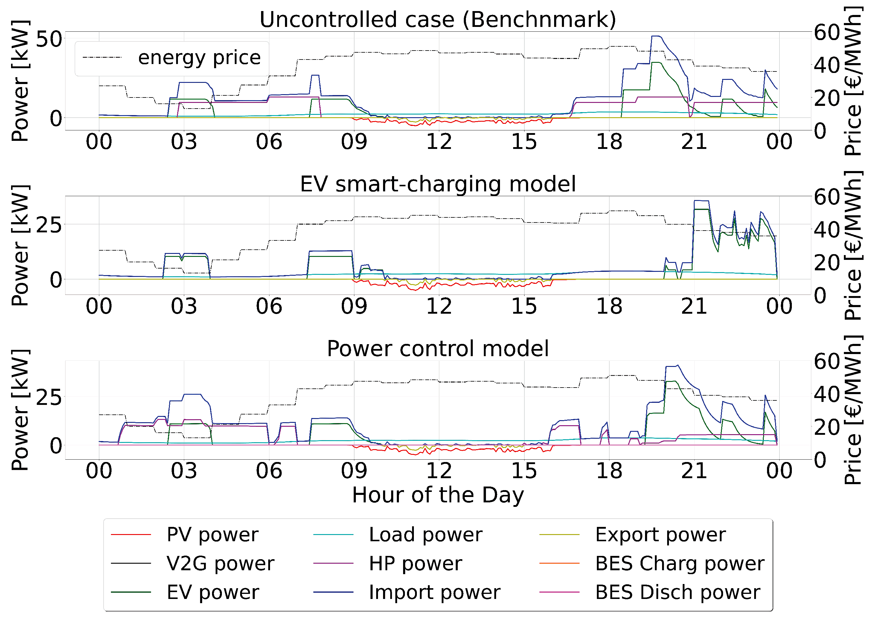
Figure 7 shows in plots (a) and (b) the power flows of nodes 2 and 6, respectively, of the large load scenario for Case 9 (BESS use during winter). Some of the previous observations from the small load scenario can also be seen here. For example, most building heating and EV charging are performed during the low energy price periods; hence, in the morning before 08:00 and in the evening after 19:00. However, in contrast with the small load scenario, less PV generation is exported to the main grid for revenues during winter, while a considerable amount is used for building heating and EV charging. Hence, in large load scales, which comprise many loads (buildings and chargers), PV self-consumption is increased, and grid power exportation is decreased. This is because when a high number of loads are constantly present at a grid, more power is consistently needed during the day, and, hence, available PV power will be firstly utilized to cover their consumption.

Regarding BESS use, BESS is hardly used in Node 2. This can be explained intuitively as follows. The BESS is constrained to have a similar SOC at the beginning and the end of the day. Hence, the amount with which it is charged during the day (e.g., during the low energy price periods) needs to be discharged during the high energy price periods. However, if during the high energy price periods, there is needed power demand for the loads and the BESS capacity is not enough to cover them, then the node needs to import grid power and cannot discharge the BESS energy to the main grid for revenues. Therefore, the high amount of loads in a large load aggregator also decreases the use of BESS, because it is preferred to use the low energy price time periods to import power for the needs of the node rather than use them to discharge the BESS to the grid for revenues. This is also validated in Figure 7b, which shows the respective power flows for Node 6 (only 6 buildings and 6 EV chargers), where BESS is considerably more utilized. Hence, it is concluded that the need for BESS is decreased when the load size is increased.

6.2.2. Power Management Cost Comparison

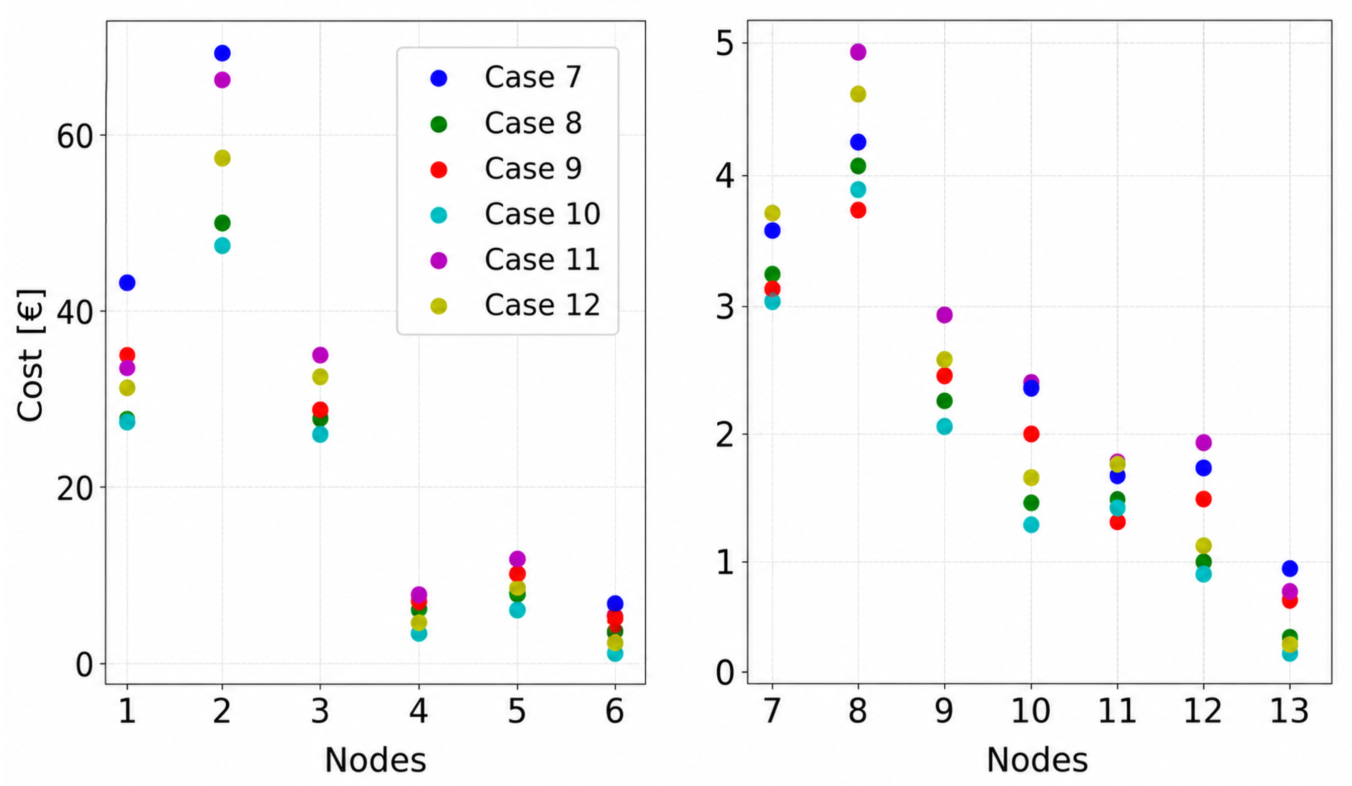
The daily energy cost for all nodes 1–13 and cases 7–12 is shown in Figure 8. As in the small load scenario, the influence of the seasonal effect is considered the most important since, for most nodes, summer cases are characterized by a lower total cost. Moreover, the total node cost always results in equal or lower values when the BESS is used, and, as a consequence, cases 9 and 10 are always less costly than their respective cases 7 and 8. Moreover, cases 8 and 10, the summer BESS cases without degradation, show the lowest total cost for almost every node. Furthermore, using BESS also closes the gap with the other cases, thus reducing the cost difference between cases with other characteristics and influencing factors. Finally, battery degradation also affects the total cost, with cases 9 and 10 always resulting in a lower cost than their respective cases 11 and 12. However, in some nodes, such as nodes 1 and 2, the contribution of the BESS for cost decrease is higher than the impact of degradation; hence, Case 7 results as the most costly case for these nodes. Nevertheless, in most of the nodes, the degradation cost is more significant, and Case 11 is the most costly case.

6.2.3. V2G Energy Comparison

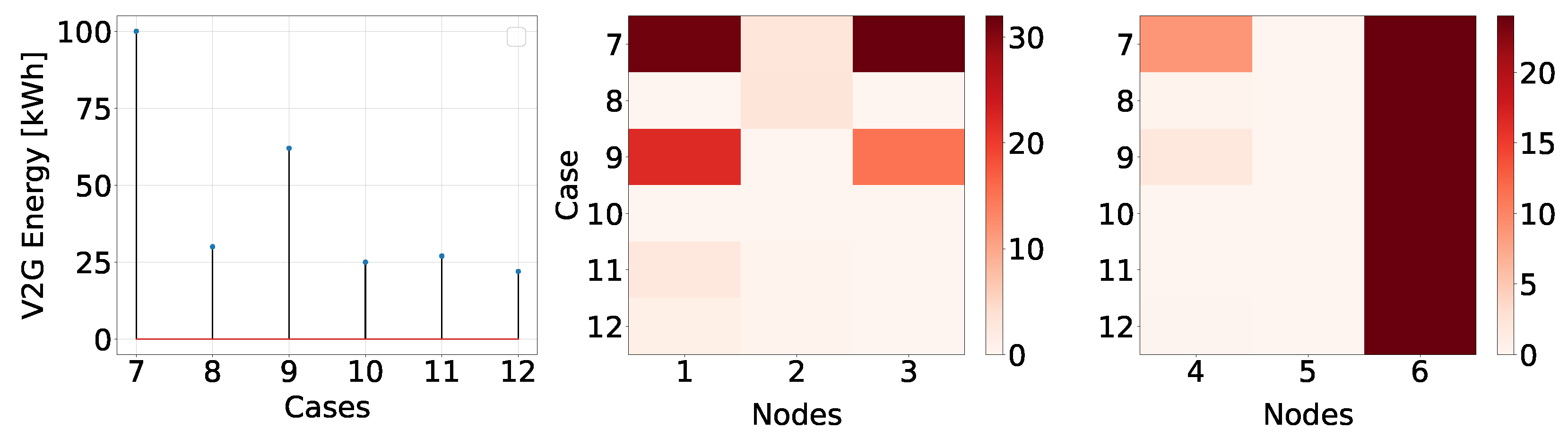
Figure 9 depicts on the left the total V2G energy used in the scenario for all cases, while the node V2G energy used is shown for the big-level nodes (1, 2, 3) and medium-level nodes (4, 5, 6) with two heatmaps on the right. As explained, V2G is more likely to be used during winter (cases 7, 9, 11) due to lower PV availability, reaching up to 100 kWh for Case 7. Moreover, introducing BESS in cases 9–12 decreases the use of V2G since BESS is preferred due to lower power losses. Furthermore, considering battery degradation decreases V2G use further (cases 11–12). Cases 7 and 9 are characterized by the highest V2G use, also in the heatmaps. Comparing Figure 9 with Figure 6b, where V2G was only used in Case 1 and slightly in Case 3, V2G is used in all cases for the large load scenario and is never zero. This is because a load aggregator of a larger size is more favorable for V2G energy use. The heatmaps also show that, excluding Node 6, larger nodes 1–3 with a higher amount of loads have more flexibility to use V2G in all cases.

6.2.4. Grid Power Exchange Comparison

Finally,

Table 10. Imported energy (Imp.) and exported energy (Exp.) in kWh: for nodes 1–13, cases 7–12.

	Case 7		Case 8		Case 9		Case 10		Case 11		Case 12
N.	Imp.	Exp.	Imp.	Exp.	Imp.	Exp.	Imp.	Exp.	Imp.	Exp.	Imp.	Exp.
1	1203.99	46.7	524.48	46.28	1647.39	487.7	527.44	55.11	927.19	73.7	644.7	180.48
2	1897.15	26.7	938.6	71.28	1864.21	43.83	924.09	88.44	2073.25	277.12	1066.84	210.47
3	889.28	13.2	517.47	27.09	1125.8	249.24	589.39	101.56	1017.74	151.74	583.02	100.1
4	244.9	17.04	111.27	20.25	248.73	20.25	152.72	60.5	294.73	68.99	131.49	44.06
5	304.86	9.39	154.09	17.82	371.7	76.31	178.61	42.51	331.28	44.11	166.68	32.58
6	194.19	10.68	68.3	20.17	281.48	98.01	101.29	54.42	255.71	71.63	66.34	22.53

summarizes the amounts of imported (Imp.) and exported (Exp.) energy for all the nodes 1–6 and cases 7–12. The imported energy greatly increases for the winter cases (150% higher for Node 1 in Case 7 than in Case 8), while the use of BESS increases imported and exported amounts at most nodes (cases 9 and 10 compared to cases 7 and 8) to use its flexibility for revenues. Moreover, the exported energy amounts are increased for all nodes in summer Case 8 compared to winter Case 7 due to the higher PV generation (e.g., 270% for Node 3). Finally, comparing the degradation cases 11 and 12 with their respective cases 9 and 10, the consideration of degradation decreases the imported and exported energy amounts for the smaller nodes; however, this is not always the case for nodes 1–3. Therefore, in larger-size nodes with a larger available BESS capacity, the PMS prefers to use its BESS capacity for revenues to compensate for the degradation cost rather than decrease the BESS equivalent cycle.

7. Discussion and Validation

7.1. Comparison with PMS Works

7.1.1. MPC Works

MPC works use the concept of the moving horizon for their control strategies. MPC models, such as this work, handle uncertainties, triggering re-optimizations of the rolling control horizon upon realization of uncertain events. A similar adaptive MPC strategy was developed in the PV–EV–BESS work in [53], where the new predicted model states are adapted at every re-optimization according to the new user preferences using a Kalman filter-based estimator. However, the modeling of various charging details, such as the CC-CV regions of the capacity degradation, was not included. MPC models that also incorporate HPs and building heating can be found in the building EMS of [36], while EVs were also added in [52]. In [52], re-optimizations are triggered at every timestep, where the new user preferences and forecasted data are fed to the mode; consequently, the control horizon moves a period T forward. While re-optimizations at every timestep provide the highest protection against uncertainties, it can become very computationally expensive if the control horizon is too long or the selected timestep is too low. The MPC models in [35,36,52] remained MILP because they considered a steady COP, i.e., the rated HP COP, the average COP over the horizon, and an approximation of the ideal COP, respectively. In this work, all cases were re-simulated with average COPS and MILP formulation (3.4 and 6 for winter and summer), finding an accuracy error increase up to 10% and computational time decrease up to 15%. On the contrary, while a variable temperature-dependent COP was considered in the building-level MPC PV–HP–TES work in [47], the HP was ON-OFF and could deliver only zero or rated heating output. In this work, the variable COP, dictated in (26), makes (28) quadratic and the PMS model MIQP. Hence, the model accuracy is increased at the expense of computational burden.

7.1.2. Multi-Objective PMS Works

There are multiple ways to solve optimization problems with multiple objectives. Rule-based strategies can be developed that adjust with rules the priority of the objectives according to the dynamic state of the problem (e.g., temperature, SOC, PV generation, load in [49]). However, these rule-based logics can become extremely complex with multiple rules and cannot find the global optima. Nash bargaining models, such as in [54], construct different subproblems for every objective and search for Pareto optimal solutions; however, they can become computationally heavy with more than two objectives. Integrating all objectives (e.g., cost, thermal comfort, emissions, etc.) with different weights in the objective, such as in [48], eliminates the computational expense of the previous methods and adjusts priorities deliberately; however, they depend on the proper weight selection. Finally, translating all objectives into one in the objective function, such as in [11,87], and this work, transforms the problem into a single simple optimization. However, it has the limitation that the objective priority depends on the resulting cost and is hardly altered.

7.2. Applicability of the PMS

The optimization of this work’s PMS has been performed from the perspective of the aggregator, which optimizes the LCTs of various LCT owners, aiming to cover their needs with the lowest cost, and communicates with the wholesale market for energy trading and the DSO for the grid constraints. Hence, regarding the perspective of the PV/EV/HP/BESS owners, the proposed PMS is directly applicable to such prosumers equipped with flexible assets such as EVs, PV systems, stationary batteries, and heat pumps. The optimization is executed locally at each node using only local measurements and forecasts together with the dynamic grid power limits communicated by the DSO. Consequently, users can minimize their electricity costs while maintaining thermal comfort and mobility requirements without requiring detailed knowledge of the distribution network. The optimization remains transparent to the user, who only needs to define comfort preferences and EV departure requirements.

Moreover, regarding the perspective of the DSO, the PMS enables the utilization of customer-side flexibility, preventing simultaneous distribution network congestion. Instead of reinforcing the network infrastructure, the DSO only communicates dynamic import/export power limits to each node based on the available grid capacity. The proposed decentralized optimization ensures that these limits are respected while maximizing the utilization of distributed energy resources. Thus, such PMS can lead to the facilitation of higher penetrations of EVs and PV systems and defer costly grid reinforcement investments.

It must be noted, though, that while the PMS requires only limited information exchange between the DSO and the prosumers, privacy issues should be carefully addressed so that the PMS is compatible with future smart-grid operation goals.

7.3. Validation

7.3.1. PMS Model

The PMS model has been validated against a rule-based uncontrolled benchmark model based on [4,69] to show the cost reduction due to control and the MPC EV smart-charging (SC) model in [87] to show its performance against other control works. The benchmark model has been created with the uncontrolled building heating model in [69], which operates the HPs only according to the desired building temperature interval [21°, 23°], and with the uncontrolled EV charging model in [4], which charges the EV fleets with rated power as soon as they arrive. It maximizes PV self-consumption according to the following rule logic:

(1) When the PV generation is higher than the total load, all the load is covered by the PV generation, and the rest of the PV power is exported to the main grid for revenues.

(2) When the total load is higher than the PV generation, all PV generation is used for its cover, and the rest is covered by imported grid power.

The MPC model in [87] performs EV charging with minimum cost and maximum self-consumption. Due to the extra features of this work, such as HP heating, the specific cost metric $C_{sp}$ in (46) has been used for the comparison (total cost C divided by the total exchanged grid power).

$$C_{sp}={\displaystyle \frac{C}{{\sum }_{t=1}^T(P_{im}^t-P_{ex}^t)}}$$

(46)

In Figure 10, the power flows of the uncontrolled, EV smart charging, and PMS models are depicted. As seen, the low energy prices during [00:00, 06:00] are not taken advantage of in the uncontrolled model as they are in the PMS model. Moreover, the EVs arrive during the energy price peak during [18:00, 20:00] and start charging immediately without avoiding the price peak, such as in the PMS. Finally, the power scheduling of the EV smart charging and PMS models is similar except for the addition of building heating. Moreover, Figure 11 depicts the comparison of nodes 1 and 2 for winter and summer between the uncontrolled model and the PMS model with and without BESS use concerning total cost and maximum needed power capacity (left plot). It can be seen that for all cases the cost is lower for the PMS model, while, in most of them, a lower power capacity is also needed. In two cases, for Node 2 during summer and winter, a higher power capacity was needed for the PMS model using BESS: 32 kW and 33 kW compared to 16 kW and 20 kW for the uncontrolled, respectively. Hence, a sensitivity analysis was realized for the power limits of these cases (right plot), proving that the PMS cost remains always lower when the same power limits are used. Finally,

Table 11. Comparison of specific cost (€/kW) for EV SC and PMS, Nodes: N1 and N2, winter–summer.

Models	Winter		Summer
	N1	N2	N1	N2
Model in [87]	3.05	3.24	4.59	4.76
Ctrl: No BESS	2.9: −4.83%	3.07: −5.25%	4.62: +0.74%	4.49: −5.81%
Ctrl: BESS	2.95: −3.09%	2.25: −30.6%	4.24: −7.56%	3.81: −20.11%

summarizes the cost comparison of the PMS and the EV SC models. The cost is highly reduced, especially when a BESS is used, reaching up to 30.6% reduction. Without the use of BESS, the specific cost of the PMS model is slightly lower (up to 5.81%), which is due to the capability of V2G use.

7.3.2. Battery Degradation Model

Validation of the original battery degradation model using experimental data has already been realized in [73] under various tests, such as storage, CC cycle, CC-CV cycle, and application-based dynamic current profile tests, founding a capacity loss error below 1% of the original capacity while the maximum relative error was below 21%.

For the validation of the linearized model, the real battery degradation has been calculated post-optimization and compared with the linear battery degradation results. Figure 12a depicts the real and linear cyclic degradation mechanisms (Qcyc 1 and Qcyc 2) and the total degradation Qcyc total for the BESS of Node 1. Moreover, the simultaneous BESS SOC and charging and discharging currents are depicted in Figure 12b. The resulting root-mean-squared error (RMSE) values are $(1.9856,1.8346,2.0652)\times {10}^{-6}$ for nodes 1–3, respectively, proving the accuracy of the developed linearized degradation model. Finally, the model’s accuracy has been validated with the models in [73,88] under 9 conditions, and the results are summarized in

Table 12. Further validation of linearized battery degradation model.

	Model [73]			Model [88]
Conditions	Calendar	Cyclic	Total	Calendar	Cyclic	Total
Condition 1	1.78%	0.67%	2.44%	1.35%	0.45%	1.8%
Condition 2	1.52%	0.79%	2.32%	1.29%	0.51%	1.8%
Condition 3	3.11%	0.74%	3.85%	1.75%	0.49%	2.23%
Condition 4	1.95%	0.76%	2.71%	1.38%	0.48%	1.86%
Condition 5	5.32%	1.96%	7.28%	10.48%	1.5%	11.98%
Condition 6	7.27%	2.15%	9.42%	11.31%	1.7%	13%
Condition 7	4.55%	2.36%	6.91%	10.06%	1.69%	11.75%
Condition 8	9.26%	2.24%	11.5%	12.1%	1.64%	13.73%
Condition 9	5.82%	2.15%	7.97%	10.68%	1.61%	12.29%

, showing an accuracy error $<3\%$ in most cases and no higher than 14%. The conditions are described below:

(1) Simulation Time (ST): 1 year (y), Battery’s year of life (YoL) 1st, Min aging.

(2) ST: 1y, YoL: ST, Min aging and avg SOC.

(3) ST: 1y, YoL: ST, Min aging and throughput (TP).

(4) ST: 1y, YoL: ST, Min aging, avg SOC, and TP.

(5) ST: 9y, YoL: 1st, Min aging.

(6) ST: 9y, YoL: 10th, Min aging.

(7) ST: 9y, YoL: ST, Min aging and avg SOC.

(8) ST: 9y, YoL: ST, Min aging and TP.

(9) ST: 9y, YoL: ST, Min aging, avg SOC, and TP.

7.4. Final Summary of Findings

Finally,

Table 13. Summary of most important findings for small-scale and large-scale load scenarios.

Scenarios	Cases	Energy Cost	Degr/Tion Cost	PV Self Cons/Tion	BESS Use	V2G Use	Imported Energy	Exported Energy	Comput. Time
Small-scale	Loads: Winter	20.3 €	0 €	73.5%	0%	9.3 kWh	562 kWh	2 kWh	38′
Small-scale	Loads/BESS: Winter	19.2 €	0 €	79%	87.5%	2.8 kWh	631 kWh	61 kWh	41′
Small-scale	Loads/BESS/ Degr/tion: Winter	17.1	4 €	80%	80%	0 kWh	675 kWh	97 kWh	62′
Small-scale	Loads: Summer	14.5 €	0 €	70.5%	0%	0 kWh	276 kWh	5 kWh	37′
Small-scale	Loads/BESS: Summer	13.2 €	0 €	74%	82.5%	0 kWh	331 kWh	63 kWh	41′
Small-scale	Loads/BESS/ Degr/tion: Summer	13.4 €	1.6 €	74%	41.3%	0 kWh	319 kWh	27 kWh	59′
Large-scale	Loads: Winter	186 €	0 €	87%	0%	100 kWh	4.78 MWh	136.1 kWh	7 h 50′
Large-scale	Loads/BESS: Winter	164 €	0 €	91%	64.5%	61 kWh	6.09 MWh	1.07 MWh	8 h 5′
Large-scale	Loads/BESS/ Degr/tion: Winter	151 €	28 €	90.5%	71.5%	26 kWh	5.39 MWh	755.9 kWh	10 h 3′
Large-scale	Loads: Summer	135 €	0 €	88%	0%	27 kWh	2.51 MWh	223.2 kWh	7 h 45′
Large-scale	Loads/BESS: Summer	128 €	0 €	91.5%	61%	25 kWh	2.72 MWh	442.7 kWh	7 h 55′
Large-scale	Loads/BESS/ Degr/tion: Summer	115 €	29 €	90%	62.5%	23 kWh	2.92 MWh	649.3 kWh	9 h 57′

summarizes all the important findings regarding the energy and degradation costs, PV self-consumption, BESS and V2G use, imported and exported energy amounts, and computational time for all case studies and load size scenarios of this work. It must be noted that $x\times 100\%$ PV self-consumption refers to the percentage of the PV generation which was used for the consumption of the loads, while $x\times 100\%$ BESS use refers to the percentage of the used BESS energy compared to the BESS equivalent cycle.

8. Conclusions

In this work, a two-level MIQP PMS model is developed for the day-ahead and real-time scheduling of PVs, EVs, HPs, and BESS for energy arbitrage respecting the grid limits. The main contributions of the PMS are, firstly, the co-integration of the LCTs and co-optimization of several related objectives, such as cost savings, PV curtailment, charging, and thermal comfort, and battery degradation, incorporating several modeling details and seeking an optimal trade-off between accuracy and computational time that is effective in both small- and large-scale load sizes. Secondly, this work contributed with a linearization and integration of a highly non-linear battery degradation model that can be extended to several empirical models of the literature. By comparing BESS and flexible loads under various conditions, it was found that while V2G is less used than the BESS in small aggregated loads due to higher power losses, opposite trends are observed in larger aggregators with a vast amount of loads; hence, the importance of BESS decreases while the load size increases. Thus, available PV generation, e.g., during summer, or stored BESS energy, and round-trip charging losses and degradation costs combined highly impact V2G usability. Moreover, the load type also has a notable impact on the flexibility of the node since commercial loads import much less grid power and use less V2G due to lower flexibility in general. Another important finding is that while degradation costs are much lower than the power management costs, they become comparable in larger load aggregators and can significantly alter the energy arbitrage decisions. Finally, the model has been compared and validated against other benchmark and control models, showing cost reductions of up to 5.81% and 30.6%, without and with BESS use, respectively.

In future work, considering more uncertainties (PV generation, weather data, load demand) is proposed to qualify the uncertainty management of the real-time scheduling level. The use of stochastic or robust optimization on Level 2 is also suggested for the enhancement of uncertainty management. Moreover, a weekly simulation is proposed to capture the intra-week effects. Finally, the dependence of the charger efficiencies on the power levels should be studied, which is expected to have a notable impact on the optimization decision-making.

References

1. Mohammad, A.; Zamora, R.; Lie, T.T. Transactive Energy Management of PV-Based EV Integrated Parking Lots. IEEE Syst. J. 2021, 15, 5674–5682. [Google Scholar] [CrossRef]
2. Arnaudo, M.; Topel, M.; Laumert, B. Vehicle-To-Grid for Peak Shaving to Unlock the Integration of Distributed Heat Pumps in a Swedish Neighborhood. Energies 2020, 13, 1705. [Google Scholar] [CrossRef]
3. European Environment Agency. Greenhouse Gas Emissions by Source Sector, EU, 2022, 2023. Available online: https://ec.europa.eu/eurostat/statistics-explained/ (accessed on 9 July 2025).
4. Damianakis, N.; Mouli, G.R.C.; Bauer, P.; Yu, Y. Assessing the grid impact of Electric Vehicles, Heat Pumps & PV generation in Dutch LV distribution grids. Appl. Energy 2023, 352, 121878. [Google Scholar] [CrossRef]
5. Brinkel, N.; Gerritsma, M.; AlSkaif, T.; Lampropoulos, I.; van Voorden, A.; Fidder, H.; van Sark, W. Impact of rapid PV fluctuations on power quality in the low-voltage grid and mitigation strategies using electric vehicles. Int. J. Electr. Power Energy Syst. 2020, 118, 105741. [Google Scholar] [CrossRef]
6. Giordano, F.; Ciocia, A.; Leo, P.D.; Mazza, A.; Spertino, F.; Tenconi, A.; Vaschetto, S. Vehicle-to-Home Usage Scenarios for Self-Consumption Improvement of a Residential Prosumer with Photovoltaic Roof. IEEE Trans. Ind. Appl. 2020, 56, 2945–2956. [Google Scholar] [CrossRef]
7. Hu, J.; Zhou, H.; Li, Y.; Hou, P.; Yang, G. Multi-time Scale Energy Management Strategy of Aggregator Characterized by Photovoltaic Generation and Electric Vehicles. J. Mod. Power Syst. Clean Energy 2020, 8, 727–736. [Google Scholar] [CrossRef]
8. Behi, B.; Baniasadi, A.; Arefi, A.; Gorjy, A.; Jennings, P.; Pivrikas, A. Cost–Benefit Analysis of a Virtual Power Plant Including Solar PV, Flow Battery, Heat Pump, and Demand Management: A Western Australian Case Study. Energies 2020, 13, 2614. [Google Scholar] [CrossRef]
9. Damianakis, N.; Yu, Y.; Mouli, G.C.R.; Bauer, P. Frequency Regulation Reserves Provision in EV Smart-Charging. In Proceedings of the 2023 IEEE Transportation Electrification Conference & Expo (ITEC), Detroit, MI, USA, 21–23 June 2023; pp. 1–6. [Google Scholar] [CrossRef]
10. Huang, S.; Wu, Q. Dynamic Tariff-Subsidy Method for PV and V2G Congestion Management in Distribution Networks. IEEE Trans. Smart Grid 2019, 10, 5851–5860. [Google Scholar] [CrossRef]
11. Vermeer, W.; Mouli, G.R.C.; Bauer, P. Optimal Sizing and Control of a PV-EV-BES Charging System Including Primary Frequency Control and Component Degradation. IEEE Open J. Ind. Electron. Soc. 2022, 3, 236–251. [Google Scholar] [CrossRef]
12. Abdelaal, G.; Gilany, M.I.; Elshahed, M.; Sharaf, H.M.; El’gharably, A. Integration of Electric Vehicles in Home Energy Management Considering Urgent Charging and Battery Degradation. IEEE Access 2021, 9, 47713–47730. [Google Scholar] [CrossRef]
13. Aljohani, T.M.; Ebrahim, A.F.; Mohammed, O.A. Dynamic Real-Time Pricing Mechanism for Electric Vehicles Charging Considering Optimal Microgrids Energy Management System. IEEE Trans. Ind. Appl. 2021, 57, 5372–5381. [Google Scholar] [CrossRef]
14. Cheng, R.; Cheng, W.; Li, J.; Chen, Z.; Shi, J.; Pan, Z.; Wu, Y.; Yu, T. Stochastic Dynamic Programming-Based Online Algorithm for Energy Management of Integrated Energy Buildings with Electric Vehicles and Flexible Thermal Loads. IEEE Access 2021, 9, 58780–58789. [Google Scholar] [CrossRef]
15. Carli, R.; Cavone, G.; Pippia, T.; De Schutter, B.; Dotoli, M. Robust Optimal Control for Demand Side Management of Multi-Carrier Microgrids. IEEE Trans. Autom. Sci. Eng. 2022, 19, 1338–1351. [Google Scholar] [CrossRef]
16. Wang, B.; Dehghanian, P.; Zhao, D. Chance-Constrained Energy Management System for Power Grids with High Proliferation of Renewables and Electric Vehicles. IEEE Trans. Smart Grid 2020, 11, 2324–2336. [Google Scholar] [CrossRef]
17. Yu, Y.; Shekhar, A.; Chandra Mouli, G.R.; Bauer, P. Comparative Impact of Three Practical Electric Vehicle Charging Scheduling Schemes on Low Voltage Distribution Grids. Energies 2022, 15, 8722. [Google Scholar] [CrossRef]
18. Tao, Y.; Qiu, J.; Lai, S. A Data-Driven Management Strategy of Electric Vehicles and Thermostatically Controlled Loads Based on Modified Generative Adversarial Network. IEEE Trans. Transp. Electrif. 2022, 8, 1430–1444. [Google Scholar] [CrossRef]
19. Wang, X.; Li, F.; Dong, J.; Olama, M.M.; Zhang, Q.; Shi, Q.; Park, B.; Kuruganti, T. Tri-Level Scheduling Model Considering Residential Demand Flexibility of Aggregated HVACs and EVs Under Distribution LMP. IEEE Trans. Smart Grid 2021, 12, 3990–4002. [Google Scholar] [CrossRef]
20. Edmunds, C.; Galloway, S.; Dixon, J.; Bukhsh, W.; Elders, I. Hosting capacity assessment of heat pumps and optimised electric vehicle charging on low voltage networks. Appl. Energy 2021, 298, 117093. [Google Scholar] [CrossRef]
21. Yilmaz, S.; Chanez, C.; Cuony, P.; Patel, M.K. Analysing utility-based direct load control programmes for heat pumps and electric vehicles considering customer segmentation. Energy Policy 2022, 164, 112900. [Google Scholar] [CrossRef]
22. Sangswang, A.; Konghirun, M. Optimal Strategies in Home Energy Management System Integrating Solar Power, Energy Storage, and Vehicle-to-Grid for Grid Support and Energy Efficiency. IEEE Trans. Ind. Appl. 2020, 56, 5716–5728. [Google Scholar] [CrossRef]
23. Ali, S.; Malik, T.N.; Raza, A. Risk-Averse Home Energy Management System. IEEE Access 2020, 8, 91779–91798. [Google Scholar] [CrossRef]
24. Wu, X.; Hu, X.; Moura, S.; Yin, X.; Pickert, V. Stochastic control of smart home energy management with plug-in electric vehicle battery energy storage and photovoltaic array. J. Power Sources 2016, 333, 203–212. [Google Scholar] [CrossRef]
25. Mateen, S.; Haque, A.; Kurukuru, V.S.B.; Khan, M.A. Discrete Stochastic Control for Energy Management with Photovoltaic Electric Vehicle Charging Station. Cpss Trans. Power Electron. Appl. 2022, 7, 216–225. [Google Scholar] [CrossRef]
26. Kazemtarghi, A.; Mallik, A. A two-stage stochastic programming approach for electric energy procurement of EV charging station integrated with BESS and PV. Electr. Power Syst. Res. 2024, 232, 110411. [Google Scholar] [CrossRef]
27. Foroozandeh, Z.; Ramos, S.; Soares, J.; Vale, Z. Goal Programming Approach for Energy Management of Smart Building. IEEE Access 2022, 10, 25341–25348. [Google Scholar] [CrossRef]
28. Imran, A.; Hafeez, G.; Khan, I.; Usman, M.; Shafiq, Z.; Qazi, A.B.; Khalid, A.; Thoben, K.D. Heuristic-Based Programable Controller for Efficient Energy Management Under Renewable Energy Sources and Energy Storage System in Smart Grid. IEEE Access 2020, 8, 139587–139608. [Google Scholar] [CrossRef]
29. Roccotelli, M.; Mangini, A.M.; Fanti, M.P. Smart District Energy Management with Cooperative Microgrids. IEEE Access 2022, 10, 36311–36326. [Google Scholar] [CrossRef]
30. Lee, J.W.; Kim, M.K. An Evolutionary Game Theory-Based Optimal Scheduling Strategy for Multiagent Distribution Network Operation Considering Voltage Management. IEEE Access 2022, 10, 50227–50241. [Google Scholar] [CrossRef]
31. Çiçek, A.; Şengör, İ.; Güner, S.; Karakuş, F.; Erenoğlu, A.K.; Erdinç, O.; Shafie-Khah, M.; Catalão, J.P.S. Integrated Rail System and EV Parking Lot Operation with Regenerative Braking Energy, Energy Storage System and PV Availability. IEEE Trans. Smart Grid 2022, 13, 3049–3058. [Google Scholar] [CrossRef]
32. Rafique, S.; Hossain, M.J.; Nizami, M.S.H.; Irshad, U.B.; Mukhopadhyay, S.C. Energy Management Systems for Residential Buildings with Electric Vehicles and Distributed Energy Resources. IEEE Access 2021, 9, 46997–47007. [Google Scholar] [CrossRef]
33. El-Taweel, N.A.; Farag, H.; Shaaban, M.F.; AlSharidah, M.E. Optimization Model for EV Charging Stations with PV Farm Transactive Energy. IEEE Trans. Ind. Inform. 2022, 18, 4608–4621. [Google Scholar] [CrossRef]
34. Zahedmanesh, A.; Muttaqi, K.M.; Sutanto, D. A Cooperative Energy Management in a Virtual Energy Hub of an Electric Transportation System Powered by PV Generation and Energy Storage. IEEE Trans. Transp. Electrif. 2021, 7, 1123–1133. [Google Scholar] [CrossRef]
35. D’Ettorre, F.; Conti, P.; Schito, E.; Testi, D. Model predictive control of a hybrid heat pump system and impact of the prediction horizon on cost-saving potential and optimal storage capacity. Appl. Therm. Eng. 2019, 148, 524–535. [Google Scholar] [CrossRef]
36. Gelleschus, R.; Böttiger, M.; Bocklisch, T. Optimization-Based Control Concept with Feed-in and Demand Peak Shaving for a PV Battery Heat Pump Heat Storage System. Energies 2019, 12, 2098. [Google Scholar] [CrossRef]
37. Duhirwe Nzivugira, P.; Hwang, J.; Ngarambe, J.; Kim, S.; Kim, K.; Song, K.; Yun, G. A novel deep learning-based integrated photovoltaic, energy storage system and electric heat pump system: Optimising energy usage and costs. Int. J. Energy Res. 2021, 45. [Google Scholar] [CrossRef]
38. Coppitters, D.; De Paepe, W.; Contino, F. Robust design optimization of a photovoltaic-battery-heat pump system with thermal storage under aleatory and epistemic uncertainty. Energy 2021, 229, 120692. [Google Scholar] [CrossRef]
39. Clift, D.; Suehrcke, H. Control optimization of PV powered electric storage and heat pump water heaters. Sol. Energy 2021, 226, 489–500. [Google Scholar] [CrossRef]
40. Facci, A.L.; Krastev, V.K.; Falcucci, G.; Ubertini, S. Smart integration of photovoltaic production, heat pump and thermal energy storage in residential applications. Sol. Energy 2019, 192, 133–143. [Google Scholar] [CrossRef]
41. Vivian, J.; Prataviera, E.; Cunsolo, F.; Pau, M. Demand Side Management of a pool of air source heat pumps for space heating and domestic hot water production in a residential district. Energy Convers. Manag. 2020, 225, 113457. [Google Scholar] [CrossRef]
42. Wakui, T.; Sawada, K.; Yokoyama, R.; Aki, H. Predictive management for energy supply networks using photovoltaics, heat pumps, and battery by two-stage stochastic programming and rule-based control. Energy 2019, 179, 1302–1319. [Google Scholar] [CrossRef]
43. Eggimann, S.; Hall, J.W.; Eyre, N. A high-resolution spatio-temporal energy demand simulation to explore the potential of heating demand side management with large-scale heat pump diffusion. Appl. Energy 2019, 236, 997–1010. [Google Scholar] [CrossRef]
44. Valinejad, J.; Marzband, M.; Korkali, M.; Xu, Y.; Al-Sumaiti, A.S. Coalition Formation of Microgrids with Distributed Energy Resources and Energy Storage in Energy Market. J. Mod. Power Syst. Clean Energy 2020, 8, 906–918. [Google Scholar] [CrossRef]
45. Good, N.; Mancarella, P. Flexibility in Multi-Energy Communities with Electrical and Thermal Storage: A Stochastic, Robust Approach for Multi-Service Demand Response. IEEE Trans. Smart Grid 2019, 10, 503–513. [Google Scholar] [CrossRef]
46. Violante, W.; Cañizares, C.A.; Trovato, M.A.; Forte, G. An Energy Management System for Isolated Microgrids with Thermal Energy Resources. IEEE Trans. Smart Grid 2020, 11, 2880–2891. [Google Scholar] [CrossRef]
47. Gasser, J.; Cai, H.; Karagiannopoulos, S.; Heer, P.; Hug, G. Predictive energy management of residential buildings while self-reporting flexibility envelope. Appl. Energy 2021, 288, 116653. [Google Scholar] [CrossRef]
48. Athanasiadis, C.L.; Papadopoulos, T.A.; Kryonidis, G.C.; Doukas, D.I. A Holistic and Personalized Home Energy Management System With Non-Intrusive Load Monitoring. IEEE Trans. Consum. Electron. 2024, 70, 6725–6737. [Google Scholar] [CrossRef]
49. Zhang, L.; Feng, G.; Huang, K.; Bi, Y.; Chang, S.; Li, A. Design and optimization for photovoltaic heat pump system integrating thermal energy storage and battery energy storage. Energy Build. 2025, 329, 115277. [Google Scholar] [CrossRef]
50. Yousefi, M.; Hajizadeh, A.; Soltani, M.N.; Hredzak, B. Predictive Home Energy Management System with Photovoltaic Array, Heat Pump, and Plug-In Electric Vehicle. IEEE Trans. Ind. Inform. 2021, 17, 430–440. [Google Scholar] [CrossRef]
51. Vermeer, W.; Chandra Mouli, G.R.; Bauer, P. Real-Time Building Smart Charging System Based on PV Forecast and Li-Ion Battery Degradation. Energies 2020, 13, 3415. [Google Scholar] [CrossRef]
52. Fotouhi Ghazvini, M.A.; Antoniadou-Plytaria, K.; Steen, D.; Tuan, L.A. Two-stage demand-side management in energy flexible residential buildings. J. Eng. 2024, 2024, e12372. [Google Scholar] [CrossRef]
53. Sen, S.; Kumar, M. Distributed-MPC Type Optimal EMS for Renewables and EVs Based Grid-Connected Building Integrated Microgrid. IEEE Trans. Ind. Appl. 2024, 60, 2390–2408. [Google Scholar] [CrossRef]
54. Li, Y.; Wang, J.; Cao, Y. Multi-objective distributed robust cooperative optimization model of multiple integrated energy systems considering uncertainty of renewable energy and participation of electric vehicles. Sustain. Cities Soc. 2024, 104, 105308. [Google Scholar] [CrossRef]
55. Huang, P.; Lovati, M.; Zhang, X.; Bales, C.; Hallbeck, S.; Becker, A.; Bergqvist, H.; Hedberg, J.; Maturi, L. Transforming a residential building cluster into electricity prosumers in Sweden: Optimal design of a coupled PV-heat pump-thermal storage-electric vehicle system. Appl. Energy 2019, 255, 113864. [Google Scholar] [CrossRef]
56. Hosseini, S.M.; Carli, R.; Dotoli, M. Robust Optimal Energy Management of a Residential Microgrid Under Uncertainties on Demand and Renewable Power Generation. IEEE Trans. Autom. Sci. Eng. 2021, 18, 618–637. [Google Scholar] [CrossRef]
57. Langer, L.; Volling, T. A Reinforcement Learning Approach to Home Energy Management for Modulating Heat Pumps and Photovoltaic Systems. Appl. Energy 2022, 327, 120020. [Google Scholar] [CrossRef]
58. Pan, T.; Zhu, Z.; Luo, H.; Li, C.; Jin, X.; Meng, Z.; Cai, X. Home Energy Management Strategy to Schedule Multiple Types of Loads and Energy Storage Device with Consideration of User Comfort: A Deep Reinforcement Learning Based Approach. Front. Therm. Eng. 2024, 4, 1391602. [Google Scholar] [CrossRef]
59. Real, A.C.; Luz, G.P.; Sousa, J.M.C.; Brito, M.C.; Vieira, S.M. Optimization of a Photovoltaic-Battery System Using Deep Reinforcement Learning and Load Forecasting. Energy AI 2024, 16, 100347. [Google Scholar] [CrossRef]
60. Felicetti, R.; Ferracuti, F.; Iarlori, S.; Monteriu, A. Peak Shaving and Self-Consumption Maximization in Home Energy Management Systems: A Combined Integer Programming and Reinforcement Learning Approach. Comput. Electr. Eng. 2024, 117, 109283. [Google Scholar] [CrossRef]
61. Latoń, D.; Grela, J.; Ożadowicz, A. Applications of Deep Reinforcement Learning for Home Energy Management Systems: A Review. Energies 2024, 17, 6420. [Google Scholar] [CrossRef]
62. Pinthurat, W.; Surinkaew, T.; Hredzak, B. An Overview of Reinforcement Learning-Based Approaches for Smart Home Energy Management Systems with Energy Storages. Renew. Sustain. Energy Rev. 2024, 202, 114648. [Google Scholar] [CrossRef]
63. Tang, X.; Chen, J.; Qin, Y.; Liu, T.; Yang, K.; Khajepour, A.; Li, S. Reinforcement Learning-Based Energy Management for Hybrid Power Systems: State-of-the-Art Survey, Review, and Perspectives. Chin. J. Mech. Eng. 2024, 37, 43. [Google Scholar] [CrossRef]
64. Zhou, H.; Zhou, Y.; Hu, J.; Yang, G.; Xie, D.; Xue, Y.; Nordström, L. LSTM-based Energy Management for Electric Vehicle Charging in Commercial-building Prosumers. J. Mod. Power Syst. Clean Energy 2021, 9, 1205–1216. [Google Scholar] [CrossRef]
65. Damianakis, N.; Kuresoo, K.; Chandra-Mouli, G.R. Battery storage integration in power systems of PVs, and flexible loads for frequency reserves provision and direct load control. Sustain. Energy Grids Netw. 2026, 47, 102404. [Google Scholar] [CrossRef]
66. Damianakis, N.; Mouli, G.R.C.; Yu, Y.; Bauer, P. Coordinated Power Control of PV Generation, Electric Mobility and Electric Heating in Different Grids. In Proceedings of the 2024 IEEE 10th International Power Electronics and Motion Control Conference (IPEMC2024-ECCE Asia), Chengdu, China, 17–20 May 2024; pp. 2082–2087. [Google Scholar] [CrossRef]
67. Lee, J.; LE, T.T.; Kim, H.; Choi, S. A Compact 17.6 kW Single-/22 kW Three-Phase Compatible EV Charger: Analysis of Active Power Decoupling, Wide Voltage Range Operation. IEEE Trans. Ind. Electron. 2025, 72, 8028–8038. [Google Scholar] [CrossRef]
68. Fermata Energy. FE-20 V2X Charger—Technical Specifications. 2026. Available online: https://www.chademo.com/products/v2g/fermata-energy-fe-20-v2x-charger (accessed on 25 June 2026).
69. Damianakis, N.; Mouli, G.C.R.; Bauer, P. Risk-averse Estimation of Electric Heat Pump Power Consumption. In Proceedings of the 2023 IEEE 17th International Conference on Compatibility, Power Electronics and Power Engineering (CPE-POWERENG), Tallinn, Estonia, 14–16 June 2023; pp. 1–6. [Google Scholar] [CrossRef]
70. Oliyide, R.O.; Cipcigan, L.M. The impacts of electric vehicles and heat pumps load profiles on low voltage distribution networks in Great Britain by 2050. Int. Multidiscip. Res. J. 2021, 11, 30–45. [Google Scholar] [CrossRef]
71. Sustainable Energy Authority of Ireland (SEAI). Heat Pumps—Technology Guide. 2020. Available online: https://www.seai.ie/sites/default/files/publications/Heat-Pump-Technology-Guide.pdf (accessed on 25 June 2026).
72. Daikin Europe N.V. Altherma Air-to-Water Heat Pump—Technical Catalogue for Installers. 2026. Available online: https://www.daikin.eu/content/dam/document-library/catalogues/heat/air-to-water-heat-pump-high-temperature/ekhbh-a/Altherma%20technical%20catalogue%20for%20installers_EPCEN08-721_Catalogues_English.pdf (accessed on 25 June 2026).
73. Schimpe, M.; von Kuepach, M.E.; Naumann, M.; Hesse, H.C.; Smith, K.; Jossen, A. Comprehensive Modeling of Temperature-Dependent Degradation Mechanisms in Lithium Iron Phosphate Batteries. J. Electrochem. Soc. 2018, 165, A181. [Google Scholar] [CrossRef]
74. ENTSO-E. Transparency Platform—Day-Ahead Prices. 2026. Available online: https://transparency.entsoe.eu/ (accessed on 25 June 2026).
75. Volta Foundation. The Battery Report 2024. Technical Report. 2025. Available online: https://volta.foundation/battery-report-2025/ (accessed on 25 June 2026).
76. Bobanac, V.; Bašić, H.; Pandžić, H. One-way voltaic and energy efficiency analysis for lithium-ion batteries. In Proceedings of the 13th Mediterranean Conference on Power Generation, Transmission, Distribution and Energy Conversion (MEDPOWER 2022), Hybrid Conference, Valletta, Malta, 7–9 November 2022; Volume 2022, pp. 261–266. [Google Scholar] [CrossRef]
77. Michalak, P. Hourly Simulation of an Earth-to-Air Heat Exchanger in a Low-Energy Residential Building. Energies 2022, 15, 1898. [Google Scholar] [CrossRef]
78. Fabrizio, E.; Monetti, V. Methodologies and Advancements in the Calibration of Building Energy Models. Energies 2015, 8, 2548–2574. [Google Scholar] [CrossRef]
79. Daikin Europe, N.V. Daikin Altherma 3—Product Catalogue. 2026. Available online: https://www.daikin.eu/ (accessed on 25 June 2026).
80. BS EN 15332:2019; Heating Boilers: Energy Assessment of Hot Water Storage Tanks. British Standards Institution: London, UK, 2019. Available online: https://knowledge.bsigroup.com/products/heating-boilers-energy-assessment-of-hot-water-storage-tanks (accessed on 25 June 2026).
81. Warmerdam, S.; Damianakis, N.; Chandra-Mouli, G.R. Power control of PV generation, flexible loads, and battery energy storage for frequency reserves provision. Sustain. Energy Grids Netw. 2026, 46, 102228. [Google Scholar] [CrossRef]
82. MFFBAS. Consumption Profiles for Electricity and Gas—Sector Documents. 2021. Available online: https://www.mffbas.nl/en/documents/ (accessed on 25 June 2026).
83. ElaadNL. Open EV Charging Data Platform. 2026. Available online: https://elaad.nl/en/data/ (accessed on 25 June 2026).
84. Meteotest AG. Meteonorm—Global Meteorological Database for Engineers, Planners and Education. 2026. Available online: https://meteonorm.com/ (accessed on 25 June 2026).
85. Enexis Groep. Open Data and Data Services. 2026. Available online: https://www.enexis.nl/over-ons/waar-staan-wij-voor/open-data (accessed on 25 June 2026).
86. Panasonic Eco Solutions Europe. Photovoltaic Module HIT® N250/N245 Datasheet. 2019. Available online: https://www.europe-solarstore.com/download/panasonic/panasonic_VBHN250SJ25_datasheet.pdf (accessed on 25 June 2026).
87. Yu, Y.; De Herdt, L.; Shekhar, A.; Mouli, G.R.C.; Bauer, P. EV Smart Charging in Distribution Grids–Experimental Evaluation Using Hardware in the Loop Setup. IEEE Open J. Ind. Electron. Soc. 2024, 5, 13–27. [Google Scholar] [CrossRef]
88. Petit, M.; Prada, E.; Sauvant-Moynot, V. Development of an empirical aging model for Li-ion batteries and application to assess the impact of Vehicle-to-Grid strategies on battery lifetime. Appl. Energy 2016, 172, 398–407. [Google Scholar] [CrossRef]
Figure 1. Description of the PMS concept: (a) Characteristics of the optimization levels of the PMS (Adapted from [65] (CC BY)). (b) Flowchart of the PMS optimization levels.
Energies 19 03582 g001
Figure 2. Example of RHO of Level 2 for daily simulation with buildings and EV chargers: Adapted from [65] (CC BY).
Energies 19 03582 g002
Figure 3. Intuitive explanation of T d e v by (30).
Energies 19 03582 g003
Figure 4. Description of the two DG scenarios: (a) Node concept and characteristics in small load scenario. (b) Distributional EMS of the large load scenario with the use of aggregators: Adapted from [81] (CC BY).
Energies 19 03582 g004
Figure 5. Small load scenario: (a) Power flow of node 3 for winter cases 1, 3, and 5. (b) Power flow of node 3 with and without BESS for summer (cases 2 and 4).
Energies 19 03582 g005
Figure 6. Small load scenario analysis: (a) Daily energy and degradation cost (lower plot) and grid power Exchange (upper plot) for nodes 1–3 and cases 1–6. (b) BESS energy use (lower plot) and V2G energy use (upper plot) for nodes 1–3 and cases 1–6.
Energies 19 03582 g006
Figure 7. Large load scenario: (a) Power flows of Node 2 for winter Case 9. (b) Power flows of Node 6 for winter Case 9.
Energies 19 03582 g007
Figure 8. Daily energy cost for nodes 1–13 and cases 7–12.
Energies 19 03582 g008
Figure 9. Total V2G energy (left) and node V2G energy for nodes 1–3 (center) and nodes 4–6 (right) for cases 7–12.
Energies 19 03582 g009
Figure 10. Comparison of power flows for the benchmark, EV SC [87], and power management algorithms: Node 1—winter.
Energies 19 03582 g010
Figure 11. Total cost and maximum used power comparison between PMS and benchmark model (Unctrl) for nodes N1–3 (left plot). Sensitivity analysis of power limits for the two specific cases (right plot).
Energies 19 03582 g011
Figure 12. Battery degradation: (a) Real and linearized cyclic battery degradation mechanisms in and post-optimization (b) Charging/discharging battery current and SOC.
Energies 19 03582 g012