Computationally Efficient Optimization of Bio-Jet Fuel Supply Chains Using Machine-Learning-Assisted Mixed-Integer Programming

Abstract

Bio-jet fuels produced from biomass-derived feedstocks represent a promising pathway for reducing the carbon intensity of aviation energy systems. However, designing supply chain networks for bio-jet fuel production requires solving large-scale mixed-integer linear programming (MILP) models that integrate facility location, feedstock allocation, material flows, and routing decisions. These models can become computationally expensive, particularly when evaluating multiple network configurations or large candidate sets of production and processing facilities. This study develops a hybrid machine learning and optimization framework to improve the computational efficiency of bio-jet fuel supply chain network design while preserving high-quality decision outcomes. The proposed iterative procedure uses supervised learning to approximate the relationship between facility location decisions and total supply chain cost. First, an initial set of supply chain configurations is generated by solving the optimization model while using randomly selected facility locations. These solutions are then used to train predictive models, including ridge regression, feed-forward neural networks, and ensemble neural networks, with facility-location configurations as inputs and total supply chain cost as the output. The trained learner is subsequently used to identify promising facility-location candidates through Thompson sampling and small-scale linear programming. These candidate solutions are evaluated by the original mixed-integer model, and the resulting observations are fed back into the learning process until convergence. Numerical experiments show that the proposed hybrid approach obtains near-optimal bio-jet fuel supply chain designs while substantially reducing computational time. For the linear case, the method achieves solutions within 0.23–0.29% of the objective function value while reducing computational time by 70.95–81.95%. For nonlinear learning models, the optimality gap decreases further to 0.13–0.15%, with computational time reductions of 45.37–60.36%. For the Texas case study and the modeling assumptions evaluated, the findings demonstrate that machine-learning-assisted optimization can reduce computational effort while preserving high-quality supply chain solutions. The extent of these benefits may vary with network size, candidate-facility structure, facility-capacity assumptions, demand characteristics, and the amount of information available to train the learning models.

1. Introduction

The transition toward lower-carbon aviation has intensified interest in bio-jet fuels derived from biomass and other renewable feedstocks. However, the viability of these fuels is shaped by more than conversion efficiency or fuel performance alone. Commercial implementation also requires an integrated supply chain capable of linking geographically dispersed feedstock resources with preprocessing sites, conversion facilities, transportation infrastructure, and final fuel demand. Recent volatility in conventional fuel markets has also reinforced the strategic value of diversifying aviation-energy supply through domestically available lower-carbon pathways. In this context, resilient sustainable aviation fuel supply chains may contribute not only to decarbonization objectives but also to longer-term energy-security and supply-diversification goals [1]. Consequently, the planning of bio-jet fuel systems is not only a technological problem but also a network design problem, where economic feasibility depends on how effectively resources, facilities, and flows are configured across space.

Mathematical optimization provides a natural framework for analyzing these network design decisions. In particular, mixed-integer linear programming (MILP) formulations can capture the discrete nature of infrastructure investment decisions together with the continuous allocation and movement of biomass, intermediates, and final fuel products. However, this modeling flexibility comes at a computational cost. As the planning problem expands to include additional regions, candidate biorefinery locations, transportation links, feedstock categories, or process alternatives, the number of decision variables and constraints can grow rapidly. This creates a practical barrier for strategic analysis, especially in settings where planners must test multiple scenarios, perform sensitivity analysis, or update the model repeatedly under changing cost, demand, or feedstock-availability assumptions.

To address this challenge, this study develops a machine-learning-assisted mixed-integer linear programming (ML-MILP) framework for biofuel supply chain network design. The approach decomposes the problem into two tasks: a supervised learning model explores strategic biorefinery-location configurations, while a reduced mathematical optimization model evaluates depot openings, biomass allocations, transportation flows, and production decisions. In doing so, the full-scale model is replaced by a sequence of reduced optimization problems, each corresponding to a candidate network configuration proposed by the learning component. 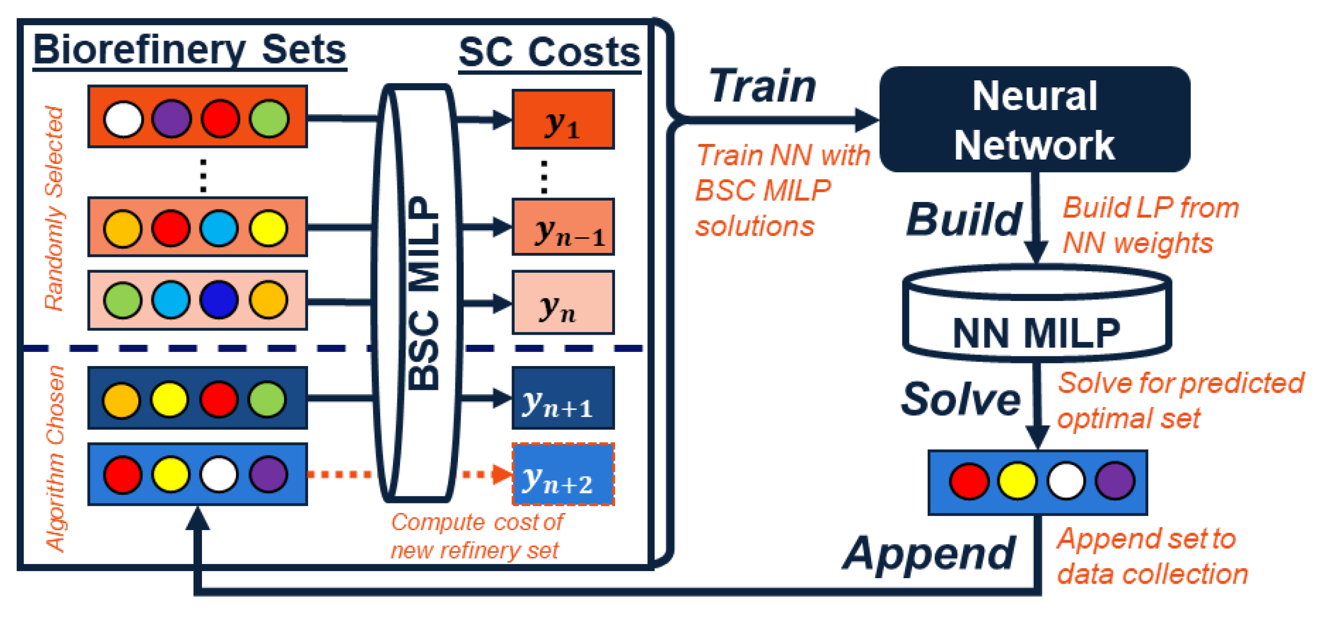Figure 1 summarizes the iterative ML-MILP workflow.

Within this framework, the optimization model serves as an evaluator of candidate decisions. For each configuration selected by the learner, the reduced model computes the associated supply chain design and returns the resulting objective function value. These evaluated configurations are then incorporated into the training set, allowing the supervised learning model to progressively approximate the relationship between strategic network-design decisions and total supply chain cost. The resulting procedure creates an iterative feedback loop in which optimization generates high-fidelity performance observations, while machine learning guides the search toward increasingly promising regions of the solution space.

In the application considered in this study, the strategic decision assigned to the learning component is biorefinery location. The learner is initially trained using solutions obtained from the reduced supply chain model under predefined biorefinery-location configurations. Based on this information, it estimates the cost implications of alternative facility-location patterns and proposes new configurations for evaluation. Although the method requires solving several reduced optimization models, each individual model is substantially smaller than the original full-scale formulation. As shown in the computational experiments, this learning-assisted decomposition can produce near-optimal biofuel supply chain designs while significantly reducing the total solution time.

The contribution of this paper is threefold. First, it presents a machine-learning-assisted solution strategy for computationally intensive mixed-integer biofuel supply chain design models. Second, it evaluates alternative supervised learning models, including linear and nonlinear predictors, for estimating the cost performance of facility-location configurations. Third, it demonstrates the computational value of the proposed framework in an industrial case study of the bio-jet fuel supply chain, showing that near-optimal solutions can be obtained with substantial reductions in computational time.

The remainder of this paper is organized as follows. Section 2 reviews the literature on biofuel supply chain optimization and learning-assisted optimization methods. Section 3 presents the mathematical formulation of the bio-jet fuel supply chain network design model. It also describes the industrial case study. Section 4 introduces the proposed learning-optimization procedures and discusses the numerical experimentation and computational performance. Finally, Section 5 concludes the paper with implications for biofuel supply chain design and future research directions.

2. Literature Review

Biofuel and biomass supply chain network design has been widely studied using mathematical programming models that integrate facility location, feedstock allocation, transportation, conversion, inventory, and demand satisfaction decisions. These models are especially relevant for strategic planning because biomass resources are geographically dispersed, transportation costs are distance-sensitive, and conversion facilities require substantial capital investment. Prior studies have formulated biomass and biofuel supply chain design problems using mixed-integer linear programming, stochastic programming, and hub-and-spoke network structures to account for facility opening decisions, material flows, conversion yields, and uncertainty in feedstock supply or demand [2,3,4,5]. Reviews of biomass-to-bioenergy and biofuel supply chain optimization have emphasized that cost-effective network design requires the simultaneous consideration of feedstock availability, preprocessing, transportation infrastructure, conversion technologies, and final fuel distribution [2,6].

A major challenge in this literature is the computational burden associated with large-scale facility location and network design models. Facility location problems are generally NP-hard, and the size of the solution space increases rapidly as the number of candidate facilities, transportation arcs, scenarios, or technology alternatives expands [7,8]. In biofuel applications, this challenge is amplified by the need to represent geographically detailed feedstock availability, multimodal transportation options, biomass quality variability, and capacity constraints. Several studies have addressed these issues through stochastic programming and decomposition-based methods. For example, Marufuzzaman et al. [3] developed a two-stage stochastic programming model for biodiesel production, while Castillo-Villar et al. [4] and Aboytes-Ojeda et al. [5] incorporated biomass quality variability into supply chain optimization models. Other work has considered price-dependent biomass availability, yield uncertainty, and climate-related storage losses [9,10,11,12]. These studies provide important modeling foundations for biofuel supply chain design, but large candidate sets and repeated scenario evaluation remain computationally demanding.

To improve computational tractability, researchers have also proposed heuristic, metaheuristic, and hybrid decomposition approaches for biomass and biofuel supply chain problems. Metaheuristics are commonly used for hard combinatorial optimization problems when exact methods become computationally expensive [13]. In supply chain and hub-location contexts, genetic algorithms, simulated annealing, and robust metaheuristic approaches have been used to search large solution spaces more efficiently [14,15]. In the biomass supply chain literature, Aboytes-Ojeda et al. [16] proposed a hybrid metaheuristic and exact-method approach for a two-stage stochastic biofuel hub-and-spoke network problem. Such approaches can reduce computational time and improve scalability, but they often require problem-specific algorithm design, parameter tuning, or specialized search operators.

More recently, machine learning has been introduced as a complementary tool for optimization and supply chain decision-making. Rather than replacing mathematical optimization, machine learning can be used to approximate expensive model components, identify promising regions of the feasible space, support policy selection, or learn decision rules from optimization outputs. Defourny et al. [17] used machine learning to support policy selection in multistage stochastic programming, while Oroojlooyjadid et al. [18] demonstrated how deep learning can integrate prediction and optimization in inventory decision-making. In biomass supply chain design, Goettsch et al. [19] developed a hybrid machine learning and stochastic MILP approach to select potential depot locations for a biomass co-firing supply chain. Their method used machine learning classifiers to screen candidate depot locations before solving the optimization model, thereby reducing the computational burden of the stochastic MILP. This work is closely related to the present study because it demonstrates the value of combining machine learning with mathematical programming in biomass supply chain network design.

Recent reviews further demonstrate the growing integration of machine learning and mathematical optimization. Scavuzzo et al. [20] reviewed machine-learning-enhanced mixed-integer linear programming methods and showed that learning-based approaches have been applied to several components of branch-and-bound algorithms, including branching, node selection, cutting-plane selection, primal heuristics, and solver configuration. Their review emphasizes that machine learning is increasingly used as a complementary mechanism for improving the efficiency of established optimization procedures rather than as a replacement for mathematical programming. Others have also expanded the methodological understanding of sustainable aviation fuel (SAF) supply chains. Liang et al. [21] systematically reviewed advances in SAF supply chain modeling and optimization, including mathematical programming, machine learning, and multi-objective approaches. They identified feedstock availability, production scalability, logistics, cost competitiveness, and policy uncertainty as continuing challenges and highlighted the need for computational methods capable of supporting integrated and scalable supply chain decisions. These recent developments reinforce the relevance of learning-assisted optimization approaches for computationally demanding SAF network-design problems.

The present study differs from prior machine-learning-assisted biomass supply chain research in how the learning component interacts with the optimization model. In Goettsch et al. [19], machine learning is used primarily as a candidate-screening mechanism to reduce the set of potential depot locations before optimization. By contrast, the proposed framework uses machine learning as an iterative decision-making component. The learner selects candidate biorefinery-location configurations, the reduced supply chain MILP evaluates those configurations, and the resulting objective-function values are incorporated into subsequent learning iterations. Thus, the proposed method treats the supply chain MILP as an expensive evaluator and reframes facility selection as a sequential learning problem. Building on preliminary work in machine-learning-assisted biofuel supply chain optimization [22], this study expands the computational analysis by evaluating additional solution procedures and comparing alternative learning-based search strategies.

Another relevant stream of literature concerns the embedding of trained machine learning models within optimization models. In particular, trained neural networks with rectified linear unit activation functions can be represented using mixed-integer linear constraints, allowing an optimization model to search over inputs that maximize or minimize the prediction of a trained neural network [23,24,25]. This capability is important for the present study because the trained neural network is not only used to estimate the relationship between biorefinery-location decisions and supply chain cost; it is also converted into an optimization model that selects the predicted best-performing combination of biorefineries.

The contribution of the present paper is therefore twofold. First, it develops an iterative machine-learning-assisted MILP framework for a bio-jet fuel hub-and-spoke supply chain network design problem. Second, it compares four learning-assisted solution procedures—ridge regression, ridge regression with Thompson sampling, neural network optimization, and ensemble neural network optimization—to evaluate the tradeoff between computational efficiency, solution quality, and model complexity. By doing so, the paper extends the biofuel supply chain optimization literature beyond exact MILP, stochastic programming, metaheuristics, and pre-optimization candidate screening, and it demonstrates how supervised learning can be used to guide facility-location decisions in a computationally expensive supply chain design problem.

To further clarify the positioning of the present study,

Table 1. Positioning of the current study relative to the prior literature.

Literature Stream	Representative Studies and Typical Approach	Gap Addressed by the Current Study
Bioenergy and biofuel supply chain optimization	Yue et al. [2]; Atashbar et al. [6]. These studies review and classify bioenergy supply chain models, planning issues, and optimization challenges.	Provides broad background on bioenergy supply chain optimization but does not propose an iterative ML-MILP solution framework.
Stochastic biofuel supply chain design	Marufuzzaman et al. [3]; Castillo-Villar et al. [4]; Aboytes-Ojeda et al. [5]. These studies use two-stage stochastic programming and decomposition-based optimization.	Models uncertainty and biomass quality variability, but does not use machine learning to guide facility-location decisions.
Biofuel network design under uncertainty	Üster and Memişoğlu [9]; Memişoğlu and Üster [10]; Geismar et al. [11]; Nur et al. [12]. These studies address biomass pricing, yield uncertainty, storage losses, and preprocessing decisions.	Addresses important sources of uncertainty, but computational acceleration through iterative learning is not the central focus.
Facility location and hub-location optimization	Owen and Daskin [7]; ReVelle and Eiselt [8]; Alumur and Kara [26]; Farahani et al. [27]. These studies establish the foundations of facility-location and hub-location modeling.	Establishes the computational difficulty of location problems, motivating learning-assisted search over candidate-facility configurations.
Metaheuristic and hybrid solution methods	Dréo et al. [13]; Xiao and Konak [14]; Ghaderi and Rahmaniani [15]; Aboytes-Ojeda et al. [16]. These studies use heuristic and hybrid methods for large-scale optimization.	Improves tractability through heuristic search, whereas the current study uses supervised learning to guide sequential biorefinery selection.
Machine-learning-assisted supply chain optimization	Defourny et al. [17]; Oroojlooyjadid et al. [18]; Goettsch et al. [19]; Keith [22]. These studies use machine learning for policy selection, inventory optimization, or candidate-location screening.	Closest prior stream. The current study goes beyond candidate screening by using machine learning iteratively to select and update biorefinery configurations based on observed MILP outcomes.
Optimization over trained neural networks	Rössig and Petkovic [23]; Tsay et al. [24]; Anderson et al. [25]. These studies develop MILP reformulations of trained ReLU neural networks.	Provides the basis for converting a trained neural network into an optimization model for selecting predicted high-performing refinery combinations.
This paper	This paper develops an iterative ML-MILP framework using ridge regression, Thompson sampling, neural network optimization, and ensemble neural network optimization.	Develops and tests an iterative-learning-guided solution framework for a Texas bio-jet fuel hub-and-spoke supply chain.

summarizes the main literature streams related to biofuel supply chain optimization, facility-location modeling, hybrid solution methods, and machine-learning-assisted optimization. The table highlights how prior studies have addressed uncertainty, biomass quality, hub-and-spoke network design, computational complexity, and neural-network reformulations. It also identifies the specific gap addressed by the present work: the development of an iterative ML-MILP framework in which machine learning does not merely screen candidate facilities before optimization, but actively guides the sequential selection of biorefinery location configurations based on observed MILP outcomes.

3. Mathematical Model and Industrial Case Study

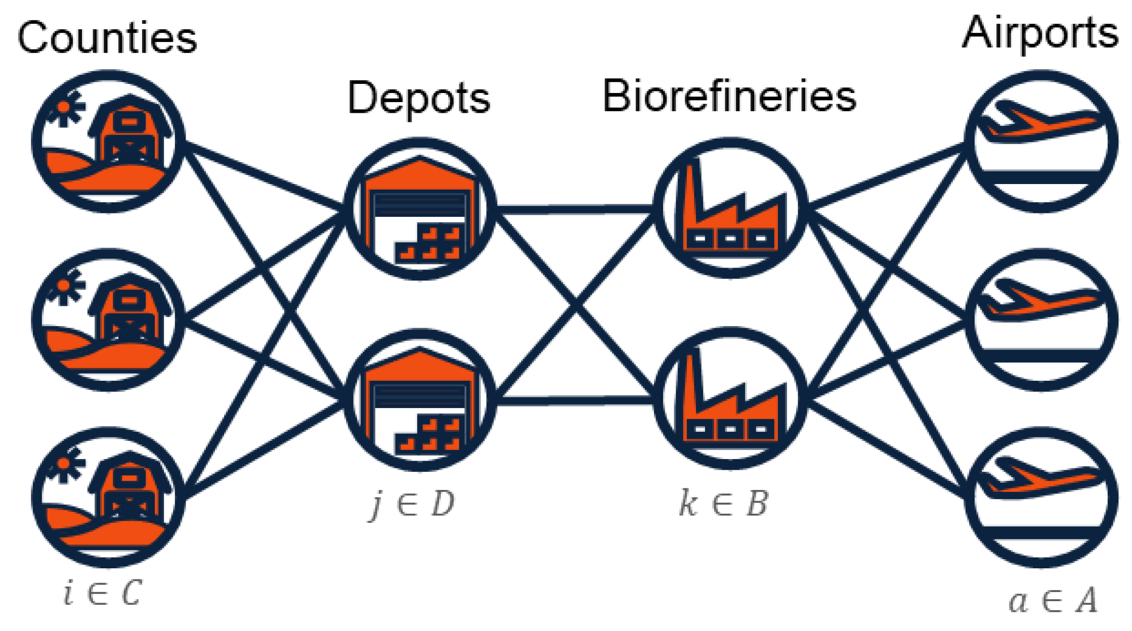
The proposed formulation models the bio-jet fuel supply chain as a hub-and-spoke network design problem that involves facility-opening and material-flow decisions. Figure 2 illustrates the structure of the supply chain. Raw switchgrass is supplied at the county level and transported by truck to candidate depot locations, where it is aggregated and densified prior to long-distance shipment. The densified biomass is then moved by rail to candidate biorefineries, where it is converted into bio-jet fuel. Finally, the produced fuel is delivered by truck to airport demand nodes. Transportation duration and traffic congestion are not explicitly modeled. All nine airport demands are represented simultaneously within a single integrated optimization problem. The model determines which depots and biorefineries to open from the available candidate sets while simultaneously optimizing biomass procurement, material flows, and fuel distribution across the entire network.

3.1. Biorefinery System, Switchgrass Feedstock, and Depot Operations

A biorefinery is an integrated processing facility in which biomass is converted into fuels, energy carriers, chemicals, and other value-added products through coordinated physical, chemical, thermochemical, or biochemical operations. Biorefineries may be differentiated by feedstock, conversion platform, product slate, and level of process integration. Within this broader context, the system considered in the present study is a biochemical lignocellulosic biorefinery supplied with switchgrass. The modeled pathway includes feedstock preprocessing, storage of biomass, the conversion process, and the final customers. The pathway is represented at the strategic supply chain level using aggregate conversion yields, facility capacities, capital costs, operating costs, and co-product credits, rather than detailed unit-operation decision variables. This representation is consistent with the scope of the study, which focuses on supply chain network design and computational performance rather than detailed process design [2,6,28].

Switchgrass was selected because it is a perennial lignocellulosic energy crop with favorable characteristics for large-scale bioenergy systems in Texas and the broader United States. Its broad climatic adaptability, relatively high biomass productivity, compatibility with marginal or lower-quality land, and comparatively modest input requirements after establishment make it a relevant candidate for regional biofuel production. In addition, switchgrass can contribute to soil conservation, long-term carbon storage, and rural economic activity while reducing direct competition with major food crops. Its suitability for a Texas supply chain also depends on the spatial distribution of feedstock resources, access to agricultural and transportation infrastructure, proximity to preprocessing and conversion facilities, and the evolving policy and market environment for low-carbon aviation fuels [2,29,30].

The model uses county-level dry biomass availability as the exogenous feedstock-supply input. Raw, non-densified switchgrass is transported from county supply nodes to selected depots, and the depot mass balance accounts for the conversion from incoming biomass to the outgoing dry, densified stream. The present formulation does not explicitly represent spatial or temporal heterogeneity in moisture content, chemical composition, ash content, particle size, or degradation during transportation and storage. Instead, these characteristics are embedded in the aggregate supply and conversion assumptions. Biomass quality variability, storage losses, and transportation-related changes in feedstock properties are important extensions for future work, particularly because they may affect usable supply, preprocessing requirements, conversion yield, and operating costs [4,5,12].

The biochemical pathway was selected because the structural carbohydrates in lignocellulosic switchgrass can be converted into intermediates that are subsequently upgraded into bio-jet fuel and co-products. The reference pathway incorporates hydrolysis, anaerobic conversion, catalytic upgrading, and lignin utilization through the 2,3-butanediol route. The process parameters used in the network model are drawn from the underlying process-design study, including a production capacity of 657,288 dry Mg/year and an overall conversion yield of 0.1323 Mg of bio-jet fuel per dry Mg of biomass [28]. Detailed pretreatment conditions, enzyme loadings, fermentation residence times, and specific microbial or yeast strains are not modeled as independent variables; rather, their combined effects are captured in the aggregate yield, capacity, capital cost, and operating cost parameters adopted from the reference design. Accordingly, the present study evaluates the supply chain implications of the selected pathway rather than optimizing its individual biochemical unit operations.

The modeled pathway should also be interpreted in light of the implementation challenges associated with lignocellulosic biochemical fuel production. Commercial deployment depends on reliable feedstock supply, effective pretreatment and hydrolysis, stable biological conversion, catalytic upgrading performance, capital availability, and the ability to manage variability at a large scale. The maturity of individual unit operations does not eliminate the integration and scale-up challenges associated with the complete pathway. For this reason, the model uses a consistent reference configuration for all candidate biorefineries and treats technology-specific process optimization and technology-readiness assessment as outside the present scope.

Depots serve as intermediate hubs for aggregation and preprocessing between geographically distributed biomass sources and centralized biorefineries. Switchgrass is transported by truck from county supply nodes to selected depots, where it is received, consolidated, preprocessed, and densified before being shipped by rail over long distances. Densification increases bulk density and improves transportation efficiency, while aggregation enables the depot to coordinate dispersed feedstock supply with the biorefinery’s larger, more stable throughput requirements. In the mathematical model, these activities are represented by depot investment costs, preprocessing capacity constraints, biomass mass-balance relationships, and the conversion of incoming non-densified biomass into an outgoing densified stream. Detailed equipment scheduling, inventory dynamics, storage degradation, and depot-level energy consumption are not explicitly modeled and are identified as opportunities for future research.

3.2. Bio-Jet Fuel Supply Chain Network Design MILP Formulation

The mixed-integer linear programming formulation presented in Equations (1)–(15) was developed for the present bio-jet fuel supply chain case study using established biomass supply chain network-design and hub-and-spoke modeling principles. The model structure builds on prior formulations that integrate geographically distributed biomass supply, facility-location decisions, preprocessing and conversion capacities, multimodal transportation, material-flow conservation, and demand satisfaction [3,4,5,16]. The present formulation adapts these general modeling concepts to the Texas bio-jet fuel system considered in this study by explicitly representing county-level switchgrass supply, intermediate depot selection and preprocessing, rail transportation of densified biomass, biorefinery-location decisions, biochemical conversion, and delivery of the resulting fuel to airport demand nodes. Accordingly, Equations (1)–(15) are not reproduced directly from a single previous study; rather, they constitute the integrated network formulation developed for the present application using parameters and process assumptions drawn from the case-study data sources described in the following subsections.

The model includes three principal groups of decision variables. The continuous variables $x_{ij}$, $y_{jk}$, and $d_{ka}$ represent, respectively, the flow of non-densified switchgrass from county i to depot j, the flow of densified biomass from depot j to biorefinery k, and the flow of bio-jet fuel from biorefinery k to airport a. The facility-location variables $W_j$ and ${\beta }_k$ indicate whether candidate depot j and candidate biorefinery k are opened, while $A_{jk}$ represents activation of the rail connection between the selected depot and biorefinery locations. The variables ${\pi }_a$ and ${\pi }_c$ represent third-party supply used to satisfy unmet fuel and co-product requirements and are penalized in the objective function. The objective in Equation (1) minimizes the combined annualized facility-investment, transportation, rail-connection, and shortage-penalty costs. Constraint (2) limits procurement by county-level biomass availability; Constraint (3) enforces the depot mass balance between incoming non-densified biomass and outgoing densified biomass; Constraints (4) and (5) impose demand satisfaction for the primary fuel and co-products; Constraints (6)–(8) impose rail, depot, and biorefinery capacity limits; Constraint (9) preserves the conversion mass balance between biomass input and fuel output; Constraint (10) links rail-connection activation to the opening of the corresponding depot and biorefinery; and Constraints (11)–(15) define the non-negativity, integrality, and binary domains of the decision variables.

• Sets:

• $\mathcal{C}$: Set of counties/suppliers, indexed by $i\in \mathcal{C}$.
• $\mathcal{D}$: Set of potential depot locations, indexed by $j\in \mathcal{D}$.
• $\mathcal{B}$: Set of potential biorefinery locations, indexed by $k\in \mathcal{B}$.
• $\mathcal{A}$: Set of airports, indexed by $a\in \mathcal{A}$.
• $\mathcal{T}$: Set of arcs from counties to depots, where $(i,j)\in \mathcal{T}$.
• $\mathcal{R}$: Set of arcs from depots to biorefineries, where $(j,k)\in \mathcal{R}$.
• $\mathcal{U}$: Set of arcs from biorefineries to airports, where $(k,a)\in \mathcal{U}$.

• Decision Variables:

• $x_{ij}$: Volume of non-densified switchgrass shipped along arc $(i,j)\in \mathcal{T}$.
• $y_{jk}$: Flow of pre-processed, densified switchgrass shipped along arc $(j,k)\in \mathcal{R}$.
• $d_{ka}$: Flow of bio-jet fuel shipped along arc $(k,a)\in \mathcal{U}$.
• $A_{jk}$: Integer variable representing the number of unit trains connecting depot $j\in \mathcal{D}$ to biorefinery $k\in \mathcal{B}$.
• ${\beta }_k$: Binary variable equal to 1 if location $k\in \mathcal{B}$ is selected as a biorefinery, and 0 otherwise.
• $W_j$: Binary variable equal to 1 if location $j\in \mathcal{D}$ is selected as a depot, and 0 otherwise.
• ${\pi }_a$: Third-party bio-diesel supply for airport $a\in \mathcal{A}$.
• ${\pi }_c$: Third-party caustic and adipic acid supply.

• Parameters:

• ${\xi }_j$: Investment cost to open a depot at node $j\in \mathcal{D}$.
• ${\varrho }_k$: Investment cost to open a biorefinery at location $k\in \mathcal{B}$.
• ${\psi }_{jk}$: Fixed cost of loading/unloading a unit train along arc $(j,k)\in \mathcal{R}$ every week for one year.
• $c_{ij}^{\mathcal{T}}$: Unit cost per metric ton shipped along arc $(i,j)\in \mathcal{T}$.
• $c_{jk}^{\mathcal{R}}$: Unit cost per metric ton shipped along arc $(j,k)\in \mathcal{R}$.
• $c_{ka}^{\mathcal{U}}$: Unit cost per metric ton shipped along arc $(k,a)\in \mathcal{U}$.
• ${\alpha }_1$: Penalty cost for demand shortage of bio-diesel.
• ${\alpha }_2$: Penalty cost for demand shortage of caustic and adipic acid.
• $s_i\left(o\right)$: Available supply in county $i\in \mathcal{C}$ under scenario $o\in \Omega$.
• ${\delta }_1$: Biomass-to-bio-jet-fuel conversion factor under anaerobic biochemical conversion.
• ${\delta }_2$: Biomass-to-caustic-and-adipic-acid conversion factor under anaerobic biochemical conversion.
• $v_{jk}$: Maximum capacity of a unit train along arc $(j,k)\in \mathcal{R}$.
• $u_j$: Pre-processing capacity of depot facility $j\in \mathcal{D}$.
• $q_k$: Production capacity of biorefinery $k\in \mathcal{B}$.
• $D_a$: Total demand for bio-diesel at airport $a\in \mathcal{A}$.
• $D_c$: Total demand for caustic and adipic acid.

The mathematical model minimizes the total costs associated with the BCS design, as shown in Equation (1). The total costs include investment costs to open depots, biorefineries, and their connecting arcs, as well as various transportation costs and demand penalty terms.

The model is formulated as a cost-minimization problem with an exogenously specified bio-jet fuel demand target rather than as a profit-maximization problem. Bio-jet fuel therefore retains inherent economic value even though sales revenue is not included explicitly in the objective function. Because the airport-demand constraints prescribe the quantity of fuel to be supplied, applying a constant selling price to every unit of required bio-jet fuel would subtract the same revenue from all solutions that satisfy the same demand and would not change the relative ranking of feasible network configurations. The objective function therefore focuses on identifying the least-cost network capable of satisfying the prescribed demand. The third-party fuel variable and its associated penalty continue to carry an economic consequence for insufficient internal production.

The secondary outputs are treated differently because their quantities are linked to biomass conversion and their market values reduce the effective net cost of the selected pathway. Accordingly, adipic acid and sodium hydroxide are represented as co-product credits rather than as evidence that the primary bio-jet fuel product lacks value.

$$Min:\sum _{j\in \mathcal{D}}{\xi }_j{W}_j+\sum _{k\in \mathcal{B}}{\varrho }_k{\beta }_k+\sum _{j\in \mathcal{D}}\sum _{k\in \mathcal{B}}{\psi }_{jk}{A}_{jk}+$$

$$\left[\sum _{i\in \mathcal{C}}\sum _{j\in \mathcal{D}}{c}_{ij}^{\mathcal{T}}{x}_{ij}+\sum _{j\in \mathcal{D}}\sum _{k\in \mathcal{B}}{c}_{jk}^{\mathcal{R}}{y}_{jk}\right.\left.+\sum _{k\in \mathcal{B}}\sum _{a\in \mathcal{A}}{c}_{kp}^{\mathcal{U}}{d}_{ka}+\sum _{a\in \mathcal{A}}{\alpha }_1{\pi }_a+{\alpha }_2{\pi }_c)\right]$$

(1)

Subject to:

$$\sum _{j\in \mathcal{D}}{x}_{ij}\le S_i\forall i\in \mathcal{C},$$

(2)

$$\sum _{i\in \mathcal{C}}(1-e_i)x_{ij}=\sum _{k\in \mathcal{B}}{y}_{jk}\forall j\in \mathcal{D},$$

(3)

$$\sum _{k\in \mathcal{B}}{d}_{ka}+{\pi }_a=D_{a}a\in \mathcal{A}$$

(4)

$$\sum _{k\in \mathcal{B}}\sum _{j\in \mathcal{D}}{\delta }_2{y}_{jk}+{\pi }_c=D_c$$

(5)

$$y_{jk}\le v_{jk}{A}_{jk}\forall j\in \mathcal{D},k\in \mathcal{B},$$

(6)

$$\sum _{i\in \mathcal{C}}\sum _{z\in \mathcal{Z}}{x}_{ijz}\le u_j{W}_j\forall j\in \mathcal{D},$$

(7)

$$\sum _{j\in \mathcal{D}}{y}_{jk}\le q_k{\beta }_k\forall k\in \mathcal{B},$$

(8)

$$\sum _{a\in \mathcal{A}}{d}_{ka}=\sum _{j\in \mathcal{D}}\delta y_{jk},\forall k\in \mathcal{B},$$

(9)

$$A_{jk}\le 0.5({\beta }_k+W_j),\forall k\in \mathcal{B},j\in \mathcal{D},$$

(10)

$$x_{ij}\ge 0\forall i\in \mathcal{C},j\in \mathcal{D},$$

(11)

$$y_{jk}\ge 0\forall j\in \mathcal{D},k\in \mathcal{B},$$

(12)

$$d_{ka}\ge 0\forall k\in \mathcal{B},a\in \mathcal{A},$$

(13)

$${\pi }_a\ge 0\forall a\in \mathcal{A},$$

(14)

$$W_j\in \{0,1\}\forall j\in \mathcal{D};{\beta }_k\in \{0,1\}\forall k\in \mathcal{B};A_{jk}\in \{0,1\}\forall j\in \mathcal{D},k\in \mathcal{B},$$

(15)

The case study retains all 254 Texas counties as potential biomass supply nodes [29]. County-level dry biomass availability for 2022 was obtained from the Billion-Ton Report [30]. The complete county set is retained because county-level biomass availability is an exogenous resource input rather than a facility-location decision. Inclusion in the set does not require a county to supply biomass; the optimization determines county participation endogenously according to available supply, transportation distance, transportation cost, depot accessibility, and the requirements of the selected network. Consequently, counties with limited biomass availability or unfavorable logistics may provide little or no biomass in the optimal solution.

The treatment of counties differs from the screening applied to candidate depots, biorefineries, and airports. Depot and biorefinery locations represent infrastructure investment decisions, and their candidate sets were narrowed using biomass proximity, transportation access, and location suitability to preserve practical relevance and computational tractability. Airports were limited to the nine largest demand centers included in the case study. Thus, the complete statewide feedstock resource base is preserved, while candidate infrastructure and final-demand nodes are screened according to their distinct roles in the network.

3.3. Depots

A shapefile provided by Oak Ridge National Laboratory was used to identify potential depot locations [31]. Train stations in the shapefile were treated as candidate depot locations, and this set was further narrowed by considering proximity to counties with relatively high biomass availability. A total of 33 potential depot locations are included in the model. The total capital investment required to open a depot is $30,178,945, with an equivalent annual cost (EAC) of $3,073,792 based on an 8% interest rate and a 20-year project life [32]. A standardized maximum preprocessing capacity of 330,000 Mg/year is used for each candidate depot to provide a consistent, representative facility scale across locations and to match the case study’s demand scope.

The standardized capacity is an upper bound rather than a required operating level. Actual depot throughput remains an endogenous model outcome determined by upstream biomass availability, transportation costs, the selected network configuration, and downstream biorefinery requirements. Therefore, an opened depot may operate below its maximum capacity. Endogenous facility sizing, discrete capacity alternatives, modular expansion, and capacity-investment decisions are outside the present scope and are identified as future extensions.

3.4. Biorefineries

Potential biorefinery locations were obtained from the Bioenergy Atlas and narrowed through a suitability analysis that emphasized proximity to railways and highways, resulting in 167 candidate locations [33]. The total capital investment for a biorefinery using hydrolysis, anaerobic conversion, catalytic upgrading, and lignin conversion through the 2,3-butanediol route is estimated at $823,698,095 in 2022 USD. The corresponding EAC plus operating cost is $208,543,998, assuming an 8% interest rate and a 20-year project life [28]. The representative production capacity is 657,288 dry Mg/year, and the conversion yield is 0.1323 Mg of bio-jet fuel per dry Mg of biomass [28]. The conversion pathway also produces monetizable co-products, namely, adipic acid and sodium hydroxide, with values of $296.5 and $31.3 per dry ton of biomass, respectively [28].

A standardized maximum biorefinery scale is used because the present study evaluates facility-location decisions under a common reference process configuration rather than optimizing facility size. As with depot capacity, the specified biorefinery capacity is an upper bound; actual throughput is determined endogenously by biomass availability, transportation costs, airport demand, and the overall network configuration. This assumption isolates the computational effects of biorefinery-location selection, which is the strategic decision assigned to the learning component. Future work may extend the formulation to include discrete technology scales, modular capacity expansion, or continuous facility-sizing decisions.

3.5. Airports

The nine most active airports in Texas, based on Federal Aviation Administration flight records for 2020, are represented as simultaneous destination nodes for the bio-jet fuel produced by the supply chain [34]. Total Texas jet-fuel consumption in 2019 was estimated at 330.2 TBtu, or 8,049,851 Mg of biofuel equivalent, according to the EIA [35]. The present supply chain is designed to satisfy 10% of this statewide demand, corresponding to 804,985 Mg of biofuel equivalent. This total is allocated among the nine airports in proportion to their respective flight activity, as shown in

Table 2. Airport demands.

Airport	Flights (2020)	Bio-Diesel Demand (Mg)
Dallas/Fort Worth (DFW)	620,831	275,493.7
George Bush t (IAH)	354,045	157,107.4
Dallas Love Field (DAL)	184,533	81,866.5
Austin-Bergstrom (AUS)	118,340	52,513.4
William P. Hobby Airport (HOU)	153,840	68,266.5
San Antonio (SAT)	165,548	73,461.9
El Paso (ELP)	83,438	37,025.6
Midland (MAF)	58,010	25,741.9
Lubbock Preston Smith (LBB)	75,466	33,488.0
Total	1,814,051	804,985

. Each airport-specific requirement is imposed concurrently through the demand constraints; the airports are not optimized independently or in separate model runs.

3.6. Transportation and Other Costs

Street distances were used for arcs $(i,j)\in \mathcal{T}$ and arc $(k,a)\in \mathcal{U}$ [36]. For arc $(j,k)\in \mathcal{R}$, railway distances were used. The cutoff point in the arcs that connect the set of counties with the depots is 170 km, as it is not recommended to ship biomass using trucks for long distances [37]. The transportation costs come in the form of linear regression results and are shown in

Table 3. Transportation costs.

Arc	Mode	Payload	Fixed Cost ($/Mg)	Variable Cost ($/(Mg*Km))	Source
$\mathcal{T}$	Truck	Raw Biomass	4.82	0.07	[38]
$\mathcal{R}$	Train	Densified Biomass	2.55	0.02	[39]
$\mathcal{U}$	Truck	Bio-Diesel	5.50	0.07	[40]

.

Of note is that the fixed transportation cost for arc $\mathcal{R}$ is very low. This is in part to utilizing unit trains in lieu of trucks but also because the fixed cost for loading and unloading the unit trains appears elsewhere in the model. This practice is in agreement with the work done by Roni [39]. In addition, the value of the co-products generated through biomass conversion, including adipic acid and sodium hydroxide, is represented as a credit that reduces the effective net cost associated with the conversion pathway and the corresponding material flows.

4. Machine Learning Solution Procedures and Computational Results

This section presents the proposed machine-learning-assisted solution procedures together with their implementation, experimental design, and comparative computational performance. Refer to Figure 1 for a visual overview of the proposed procedures.

The algorithm starts with an initial sample of solutions to the supply chain optimization problem where the refineries are randomly selected. The choice of nine biorefineries is a simplifying hypothesis specific to this case study rather than a general property of the algorithm. It is supported by the demand-to-capacity structure and cost parameters of the instance. Each biorefinery has an annual capacity of (657,88) dry Mg, which, at a conversion yield of (0.1323) Mg of fuel per dry Mg, corresponds to approximately (86,960) Mg of bio-jet fuel per facility. Given an aggregate demand of (804,985) Mg, satisfying demand exclusively through the biorefinery network would require 804,985/86,960 = 10 facilities. Nine facilities, however, supply approximately (97.2%) of total demand, with the remaining (2.8%) covered through third-party supply at a penalty cost. Because the annualized cost of opening an additional biorefinery substantially exceeds the penalty associated with covering this limited residual demand, the cost-minimizing solution opens nine facilities. This result is consistent with the optimal facility count obtained from the exact full-scale MILP benchmark. The facility cardinality enters the proposed method only through the parameter $\mathrm{\Psi }$ in the selection step. The framework is therefore not restricted to $\mathrm{\Psi }$ = 9. For instances with different demand, capacity, and cost structures, the ratio (D/q) may be used to identify an economically plausible neighborhood of candidate cardinalities. When the optimal cardinality is uncertain, the method can be applied over a narrow integer range of $\mathrm{\Psi }$, and the solution yielding the best exact-MILP objective value can be retained.

From there, a regression-type model is fit to the collection of solutions, and the best refineries for the next run are determined via the fit regression model. The selected refineries are then fed into the supply chain optimization model to generate an additional feature-response pair, which is then used to fit a new regression. This process is iterated on to achieve the final result. Four learning-assisted procedures are evaluated: L1 (ridge regression), L2 (ridge regression with Thompson sampling), NL1 (neural network), and NL2 (ensemble neural network).

Table 4. Overview of machine learning solution procedures.

Regression Algorithm	Initial Sample	Model and Hyperparameter Design	Selection Strategy
L1: Ridge Regression	30 SC optimization solutions with randomly selected refineries	Ridge regression with $\lambda =0.1$	Select refineries corresponding to maximal regression coefficients
L2: Ridge Regression with Thompson Sampling	30 SC optimization solutions with randomly selected refineries	Ridge regression with $\lambda =0.1$	Vary refineries via Thompson sampling then select refineries corresponding to maximal post-varied regression coefficients
NL1: Neural Network	30 SC optimization solutions with randomly selected refineries	NN with one hidden layer with 15 nodes	MILP used to select the best performing combination of refineries
NL2: Ensemble Neural Network	30 SC optimization solutions with randomly selected refineries	Ensemble NN with one hidden layer with 15 nodes and 10 folds	MILP used to select the best performing combination of refineries based on average performance across all folds

summarizes the common initial sample, model design, and selection strategy for each procedure according to the framework shown in Figure 3.

4.1. Regression Overview

Of paramount importance to the suggested solution procedure is how to frame the results of the supply chain optimization problem as a regression algorithm suitable for machine learning. For the regression algorithms in this work, the I/O is as follows:

Features: X

• $x_{ij}$ takes the value 1 if refinery j was selected for run i of the supply chain optimization model and 0 otherwise.

Responses: $y^{\ast }$

• $y_i^{\ast }$ denotes the savings generated by the combination of selected refineries for run i of the supply chain optimization model. It is computed according to the following formula $y_i^{\ast }=C-y_i$, where C is the solution to the supply chain optimization problem if no refineries are opened and $y_i$ is the solution to the supply chain optimization problem for the selection of refineries used for run i.

The problem is framed in this way to generate an environment where the maximal regression coefficients are desirable as they denote the refineries that generate the most savings. For linear regression, this is the mathematical equivalent of imposing a known intercept.

What follows is a discussion of the development and implementation of the four machine-learning-based algorithms in the present work.

4.2. Linear Methods

4.2.1. L1: Ridge Regression

The linear methods utilize ridge regression in order to determine the regression coefficients for the potential biorefinery locations. While as much data as desirable are available to be generated since the problem is such that data are created via runs of the optimization model, the desired experimental outcome is a reduction in computational burden; thus, the algorithms to be utilized should strive to perform well in a limited data environment.

Each configuration is represented by 167 binary location variables, whereas each trial contains 300 feature-response pairs. In addition, all feasible configurations satisfy a fixed-cardinality constraint, which induces dependence among the predictors. This relatively low sample-to-feature ratio and the resulting multicollinearity motivate the use of ridge regression rather than ordinary least squares. Ridge regularization stabilizes the coefficient estimates and reduces their sensitivity to correlated predictors through the estimator. The problem setup coupled with numerical experimentation indicates that the regression coefficients can be applied analytically via the formula below:

$$\beta ={(X^{T}X+\lambda I)}^{-1}{X}^T{Y}^{\ast }$$

(16)

The penalty term $\lambda I$ ensures a stable and uniquely defined estimate even when the predictor matrix is poorly conditioned and shrinks weak or unstable coefficients. The ridge model is therefore used as a regularized decision-support model rather than as an unrestricted global predictor of supply-chain cost.

Once the coefficients have been obtained the next step in the solution procedure is to determine the predicted maximal performing set of biorefineries. For this, we leverage problem knowledge derived from supply and capacity considerations as well as numerical experiments to impose that a good solution should contain 9 biorefineries. With this in mind, the maximal performing set according to the regression will simply be the refineries corresponding to the nine largest regression coefficients. This regression and maximal set determination scheme constitutes the approach for the first solution procedure. This procedure is outlined in Algorithm 1.

Algorithm 1 L1: Ridge-regression-powered solution procedure:

Initialize: ${\beta }_0$

for $t=0,\dots ,T-1$ do

Compute: $x_{t+1}\leftarrow argma{x}_{{\beta }^{\prime }\subset \beta ,\left|{\beta }^{\prime }\right|=9}{\sum }_{i\in {\beta }^{\prime }}{\beta }_i$

Observe: $y_{t+1}$

Update: ${\beta }_{t+1}$

end for

4.2.2. L2: Ridge Regression with Thompson Sampling

As will be demonstrated, this formulation is primed to suffer from an information exploitation problem where we start with a limited amount of data using multiple linear regression to predict the best-performing input and iterate from there. To combat this, L2 introduces Thompson Sampling to promote exploration while retaining the same ridge-regression structure. The scale parameter $\eta$ was set based on a small preliminary grid search over values on either side of unity (e.g., $\eta \in \{0.25,0.5,1,2,4\}$), evaluated by the resulting optimality gap and its variance across trials. The second solution procedure begins the same as the first with the analytical computation of regression coefficients via ridge regression. From here, a normal distribution is imposed centered around each coefficient with a standard deviation related to the mean squared error (MSE) of the regression and the variance of the input. New coefficients are randomly sampled from these distributions via the equation below, where $\eta$ is a scale parameter:

$${\beta }_i^{\ast }=normrand({\beta }_i,\eta \sqrt{{\displaystyle \frac{MSE}{diag{\left(X^{T}X\right)}_i}}})$$

(17)

Once the new coefficients have been obtained, the process to select the predicted maximal performing set of refineries is the same as above in that the 9 largest coefficients indicate the refineries that the regression thinks should be selected. This approach is outlined in Algorithm 2.

Algorithm 2 L2: Ridge Regression with Thompson sampling-powered solution procedure

Initialize: ${\beta }_0$

for $t=0,\dots ,T-1$ do

Vary: ${\beta }_t^{\ast }\leftarrow {\beta }_t$

Compute: $x_{t+1}\leftarrow arg{max}_{{\beta }^{\ast \prime }\subset {\beta }^{\ast },|{\beta }^{\ast \prime }|=9}{\sum }_{i\in {\beta }^{\ast \prime }}{\beta }_i^{\ast }$

Observe: $y_{t+1}$

Update: ${\beta }_{t+1}$

end for

4.3. Non-Linear Methods

The biorefinery-location problem is combinatorial because the selected facilities operate jointly to satisfy regional demand. The additive structure of the linear procedures does not fully capture these interactions. The nonlinear procedures therefore use neural networks to represent interactions among selected biorefineries and predict the savings associated with complete facility configurations.

4.3.1. NL1: Neural Network Optimization Algorithm

NL1 uses a relatively small feed-forward neural network because the training data are intentionally limited. The network contains one fully connected hidden layer with 15 nodes and rectified linear unit (ReLU) activation functions. The hidden layer is fully connected to an output node that predicts supply chain savings. Because the model is intended to capture nonlinear interactions, selecting facilities independently according to a simple ranking would not preserve the full learned relationship. Instead, the trained ReLU network is reformulated as an MILP to select the combination of biorefineries that yields the highest predicted savings [23].

• Sets:

• $\mathcal{K}$: Set of hidden-layer nodes, indexed by $k\in \mathcal{K}$.
• $\mathcal{I}$: Set of features corresponding to potential biorefinery locations, indexed by $i\in \mathcal{I}$.
• $\mathcal{C}$: Set of feasible biorefinery selections, defined as $\mathcal{C}=\{X=(x_1,x_2,\dots ,x_n)\mid {\sum }_{i\in \mathcal{I}}{x}_i=\mathrm{\Psi }\}$.
• $\mathcal{O}$: Set of folds, indexed by $o\in \mathcal{O}$.

• Parameters:

• $m_{ik}\left(o\right)$: First-layer weight from feature i to hidden node k for fold $o\in \mathcal{O}$.
• $b_k\left(o\right)$: Hidden-layer bias for node k for fold $o\in \mathcal{O}$.
• $n_k\left(o\right)$: Output-layer weight from hidden node k for fold $o\in \mathcal{O}$.
• $\mathrm{\Psi }$: Number of refineries to be selected.
• $U_k\left(o\right)$: Upper bound for the ReLU reformulation, defined as

  $$U_k\left(o\right)=\underset{X\in \mathcal{C}}{sup}\left\{\sum _{i\in \mathcal{I}}{m}_{ik}\left(o\right)x_i+b_k\left(o\right),1\right\},\forall k\in \mathcal{K},\forall o\in \mathcal{O}.$$
• $L_k\left(o\right)$: Lower bound for the ReLU reformulation, defined as

  $$L_k\left(o\right)=\underset{X\in \mathcal{C}}{inf}\left\{\sum _{i\in \mathcal{I}}{m}_{ik}\left(o\right)x_i+b_k\left(o\right),-1\right\},\forall k\in \mathcal{K},\forall o\in \mathcal{O}.$$

• Decision Variables:

• $a_k\left(o\right)$: Value passed to hidden node k for fold $o\in \mathcal{O}$.
• $h_k\left(o\right)$: ReLU-corrected value passed from hidden node k for fold $o\in \mathcal{O}$.
• $x_i$: Binary variable equal to 1 if refinery $i\in \mathcal{I}$ is selected and 0 otherwise.
• $y_k\left(o\right)$: Binary variable used for the ReLU reformulation for hidden node k and fold $o\in \mathcal{O}$.

$$maxR={\displaystyle \frac{1}{\left|\mathcal{O}\right|}}\sum _{o\in \mathcal{O}}\sum _{k\in \mathcal{K}}{n}_k\left(o\right)h_k\left(o\right)$$

(18)

Subject to:

$$\begin{array}{cc}\hfill \sum _{i\in \mathcal{I}}{x}_i& =\mathrm{\Psi },\hfill \end{array}$$

(19)

$$\begin{array}{cccc}\hfill \sum _{i\in \mathcal{I}}{m}_{ik}\left(o\right)x_i+b_k\left(o\right)& =a_k\left(o\right),\hfill & \hfill & \forall k\in \mathcal{K},\forall o\in \mathcal{O},\hfill \end{array}$$

(20)

$$\begin{array}{cccc}\hfill a_k\left(o\right)& \le h_k\left(o\right),\hfill & \hfill & \forall k\in \mathcal{K},\forall o\in \mathcal{O},\hfill \end{array}$$

(21)

$$\begin{array}{cccc}\hfill h_k\left(o\right)& \le U_k\left(o\right)y_k\left(o\right),\hfill & \hfill & \forall k\in \mathcal{K},\forall o\in \mathcal{O},\hfill \end{array}$$

(22)

$$\begin{array}{cccc}\hfill h_k\left(o\right)& \le a_k\left(o\right)-L_k\left(o\right)(1-y_k\left(o\right)),\hfill & \hfill & \forall k\in \mathcal{K},\forall o\in \mathcal{O},\hfill \end{array}$$

(23)

$$\begin{array}{cccc}\hfill L_k\left(o\right)& \le a_k\left(o\right)\le U_k\left(o\right),\hfill & \hfill & \forall k\in \mathcal{K},\forall o\in \mathcal{O},\hfill \end{array}$$

(24)

$$\begin{array}{cccc}\hfill y_k\left(o\right)& \in \{0,1\},\hfill & \hfill & \forall k\in \mathcal{K},\forall o\in \mathcal{O},\hfill \end{array}$$

(25)

$$\begin{array}{cccc}\hfill x_i& \in \{0,1\},\hfill & \hfill & \forall i\in \mathcal{I}.\hfill \end{array}$$

(26)

Thus, the solution approach for the NL1 neural network solution procedure can be seen in Algorithm 3. The procedure begins with a set of refinery/solution pairs and a fit neural network denoted by ${\theta }_0$. At each step, the next set of refineries ($x_{t+1}$) is selected by solving the above optimization problem. Then the SC solution given that set of refineries ($y_{t+1}$) is determined by solving the supply chain MILP. This refinery/solution pair is then added to the dataset, and the neural network is refit ${\theta }_{t+1}$ before the next iteration.

Algorithm 3 NL1: Neural-network-powered solution procedure:

Initialize: ${\theta }_0$

for $t=0,\dots ,T-1$ do

Optimize: $x_{t+1}=argmaxR\left({\theta }_t\right)$

Observe: $y_{t+1}$

Update: ${\theta }_{t+1}$

end for

4.3.2. NL2: Ensemble Neural Network

Extending this solution procedure in the same vein as the linear case with Thompson sampling is not without its challenges. Computing the posterior distribution of the fit neural network can be challenging or even intractable. For this reason, NL2 adopts the approach of Lu and Roy in that an ensemble neural network is used instead of Thompson sampling [41]. In this approach, we apply 10 folds to the data and omit a random 10% of the data each step to generate 10 distinct datasets that are each fitted with a neural network structured as above. In this scenario, the next set of refineries constitutes those that have the average maximal performance across the 10 networks. The algorithm for this ensemble approach is shown below in Algorithm 4.

Algorithm 4 NL2: Ensemble-neural-network powered solution procedure:

Initialize: ${\theta }_0^1,\dots ,{\theta }_0^{10}$

for $t=0,\dots ,T-1$ do

Optimize: $x_{t+1}=argmaxR({\theta }_t^1,\dots ,{\theta }_t^{10})$

Observe: $y_{t+1}$

Update: ${\theta }_{t+1}^1,\dots ,{\theta }_{t+1}^{10}$

end for

4.4. Software Implementation and Solver Selection

The optimization model is implemented in Julia using JuMP and solved with IBM CPLEX under a 0.5% optimality-gap tolerance. Regression model estimation and refinery-location selection are performed in MATLAB R2023b, version 23.2 using the Statistics and Machine Learning Toolbox and the Deep Learning Toolbox. The complete iterative algorithm is coordinated in Julia, with MATLAB routines called through the MATLAB.jl package for the learning and selection components.

MATLAB was selected because it provides an integrated environment for numerical experimentation, matrix operations, machine-learning implementation, visualization, reproducible scripting, and direct interaction with external optimization workflows. CPLEX was selected because the study requires repeated solutions of large MILP formulations and a reliable benchmark for exact solvers. Its mature branch-and-cut algorithms, presolve capabilities, numerical diagnostics, solver controls, and established integration with algebraic modeling environments make it suitable for evaluating the computational performance of the proposed procedures. Commercial software also has disadvantages, including licensing costs, access restrictions, and potential barriers to reproducibility. Open-source alternatives, including Python 3.11-based scientific and machine-learning libraries, together with solvers such as HiGHS, SCIP, and CBC, may improve accessibility and reproducibility, although computational performance, supported features, licensing terms, and integration effort may differ across platforms. The proposed ML-MILP framework is platform- and solver-independent in principle; MATLAB and CPLEX are implementation choices rather than methodological requirements.

4.5. Experimental Design and Benchmark

All proposed procedures are benchmarked against the full supply chain optimization model, which yields an objective-function value of $2,316,428,200 and requires 3599 s of computational time.

The proposed method follows an online, active-learning design rather than an offline supervised-learning pipeline, which governs how the data are handled. Each trial begins with an initial design of 30 feature–response pairs obtained by solving the exact supply chain MILP for randomly selected refinery configurations. At each subsequent iteration the current surrogate proposes one configuration, that configuration is evaluated by the exact MILP, and the resulting pair is appended to the accumulated data on which the surrogate is refit; 270 iterations therefore yield 300 pairs per trial, repeated over 10 independent trials. Because configurations are generated and labeled on the fly, there is no fixed held-out test set because all newly generated observations are incorporated sequentially into model updating. The exact MILP instead provides full-fidelity evaluation of every recommended configuration and supports assessment of downstream decision quality. Solution quality is accordingly certified by the optimality gap of the returned design relative to the exact benchmark (

Table 5. Detailed performance of the algorithms’ solutions.

Algorithm	Mean Solution Value	Difference to Optimal	Standard Deviation
L1: Ridge Regression	$2,323,060,838	0.29%	$2,254,306
L2: Ridge Regression with Thompson Sampling	$2,321,666,012	0.23%	$1,184,592
NL1: Neural Network	$2,319,825,893	0.15%	$1,072,780
NL2: Ensemble Neural Network	$2,319,507,373	0.13%	$1,181,481

and

Table 6. Detailed performance of algorithms’ computational time.

Algorithm	Mean Time Obtained	Time Reduction	Standard Deviation
L1: Ridge Regression	650 s	81.95%	217 s
L2: Ridge Regression with Thompson Sampling	1045 s	70.95%	518 s
NL1: Neural Network	1427 s	60.36%	313 s
NL2: Ensemble Neural Network	1966 s	45.37%	362 s

) rather than by surrogate fit on auxiliary data. Generalization is controlled within each surrogate: the linear models use ridge regularization ($\lambda$ = 0.1) to control coefficient instability and multicollinearity in the limited-data setting, and the ensemble neural network uses a resampling scheme equivalent to cross-validation, training ten networks each on a subset omitting a random 10% of the data and selecting configurations by their average predicted performance across folds.

The surrogate models are not intended to provide globally accurate predictions of supply-chain cost across the entire feasible space. Their purpose is to rank or select promising refinery configurations that are subsequently evaluated at full fidelity using the original MILP. Accordingly, the primary performance criterion is the optimality gap between the best MILP-evaluated configuration returned by each procedure and the exact benchmark, as reported in Table 5 and Table 6. Conventional predictive metrics such as MSE, MAE, and $R^2$ assess pointwise predictive accuracy on unseen observations, whereas the optimality gap directly evaluates the quality of the optimization decisions produced by the surrogate-assisted procedure.

The effective learning problem is also more structured than the nominal feature count alone suggests. Feasible observations are restricted to configurations containing exactly $\mathrm{\Psi }$ active locations, ridge regularization shrinks unstable coefficients, and the sequential design progressively concentrates evaluations in more promising regions of the solution space. The linear models therefore use ridge regularization with $\lambda =0.1$ to control coefficient instability under the limited-data setting. The ensemble neural-network procedure further reduces sensitivity to individual training samples by fitting ten models to resampled subsets of the accumulated data and selecting configurations according to their average predicted performance.

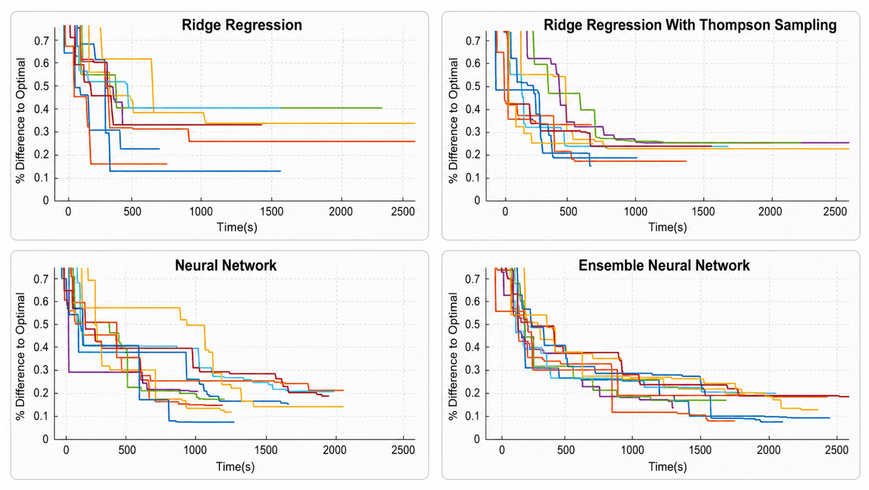
Figure 3 contains the best solution represented as a percent difference from the optimal solution observed in the process up to the current time. The benchmark objective value is not available to the learning algorithms and does not influence model fitting, candidate selection, or stopping. Instead, every proposed configuration is evaluated by the original supply chain MILP, and the gap to the benchmark is calculated ex post solely to compare the quality and convergence behavior of the four procedures. The linear methods converge faster than the nonlinear ones as expected due to the additional computational complexity of fitting a NN as opposed to analytical linear coefficients. Additionally, the introduction of Thompson Sampling does slow the convergence rate of the ridge regression but appears to greatly reduce solution variance. Both linear methods converge rather quickly but we do observe some cases where the Thompson Sampling kicks the solutions out of a steady state and obtains a lower solution value.

For the nonlinear methods, it is visually difficult to distinguish between the best solutions; however, the ensemble NN exhibits more uniform convergence behavior. The progressive reduction in optimality gap indicates that the sequential procedures identify increasingly competitive configurations; however, this pattern should not be interpreted as an independent measure of out-of-sample predictive accuracy.

For a deeper dive into performance as it pertains to solution integrity, Table 5 details statistics for the best solutions obtained from each algorithm over each of the 10 trials.

From a mean solution value standpoint, it can be seen that, with each increase in algorithmic complexity, we see a reduction in the gap to the optimal solution. The ability of the NN approaches to capture the nonlinear effects associated with the combinatorial optimization problem that is the selection of biorefinery locations really is highlighted here. From a solution variance perspective, we see that the basic ridge regression has roughly double the solution variance of the other methods.

4.6. Computational Performance

The computational performance is summarized in Table 6. The reported time is an end-to-end measure beginning with the generation of the initial random MILP sample and ending at the first occurrence of the best solution obtained during a run. Consequently, the reported values include all computational activities required by each procedure, including surrogate-model fitting, refinery-configuration selection, evaluation of selected configurations using the original supply chain MILP, iterative data updating, and implementation overhead. The values should therefore not be interpreted as the execution time of a single iteration or of an individual model component.

This phenomenon is crucial for practitioners that seek to implement this algorithm, as early termination of the algorithm may lead to a lower quality solution than what was possible. As for the nonlinear methods, we see an increase in time from the linear ones as not only do we have to fit a NN, or 10, for each iteration but also have to solve a MILP to determine the predicted optimal set of biorefineries. With that being said, we still observe significant time savings as opposed to solving the full problem.

The comparisons reported in Table 5 and Table 6 are interpreted as descriptive measures of computational performance rather than as evidence of statistical superiority among the proposed methods. The primary objective of the analysis is to characterize the practical tradeoff between solution quality and computational effort under the conditions of the Texas case study. Accordingly, emphasis is placed on the magnitude of the observed optimality gaps, computational-time reductions, and run-to-run variability. Statistical significance alone does not measure the magnitude or practical relevance of an observed difference [42]. For example, NL2 achieved a mean optimality gap of 0.13%, compared with 0.15% for NL1, while requiring a greater mean computational effort. Similarly, L1 produced the largest mean optimality gap among the four methods, 0.29%, but achieved the greatest computational-time reduction, 81.95%. These results indicate a tradeoff between solution quality and computational efficiency rather than a universal ranking of the methods. The observed differences should therefore be interpreted within the scope of the evaluated case study, algorithm settings, and 10 independent experimental trials.

Stringing all of this together, the basic Ridge-Regression-powered solution procedure is able to produce a near-optimal solution with very little computational effort. This approach, however, has high variance in solutions due to the under-determined nature of the problem. To remedy this, Thompson Sampling can be employed at the cost of the computational burden. This implementation will lower the solution variance and mean, thus yielding better performance from an optimality standpoint. The next step in increasing performance can be realized from the introduction of an NN that is able to capture the nonlinear effects associated with the combinatorial optimization problem of biorefinery location selection. Additionally, an ensemble NN has the potential to even further reduce the optimality gap.

5. Conclusions and Future Work

This study proposed a hybrid machine learning and mixed-integer linear programming (ML-MILP) solution framework for computationally intensive bio-jet fuel supply chain network design problems. The proposed approach reduces the computational burden of the full MILP formulation by transferring part of the facility-location search process to a supervised learning algorithm. Instead of solving the complete optimization problem directly, the method iteratively evaluates selected facility-location configurations through a reduced MILP model, uses the resulting objective function values to train a predictive model, and then identifies new candidate configurations with strong expected performance.

Four algorithmic variants were developed and evaluated: two based on linear learning models and two based on nonlinear learning models. These approaches were applied to a hub-and-spoke bio-jet fuel supply chain design problem in the state of Texas, where counties serve as biomass supply nodes, depots perform densification, biorefineries convert densified biomass into bio-jet fuel, and airports represent demand locations. The computational results show that all proposed methods were able to generate near-optimal supply chain designs while reducing solution time relative to solving the full optimization problem through exact methods. The nonlinear methods achieved smaller optimality gaps than the linear approaches, although this improvement came with higher computational requirements. This trade-off suggests that the selection of a learning model should depend on the decision context: linear models may be preferable when computational speed and interpretability are priorities, whereas nonlinear models may be more appropriate when marginal improvements in solution quality justify additional computational effort.

From a managerial perspective, the proposed framework provides a practical decision-support tool for strategic biofuel infrastructure planning. Bio-jet fuel supply chains involve high-capital, long-horizon decisions, including where to locate depots and biorefineries, how to allocate biomass resources, and how to route materials through the network. In practice, decision-makers often need to evaluate multiple scenarios involving feedstock availability, demand growth, transportation costs, policy incentives, technology assumptions, or regional development objectives. The economic deployment of bio-jet fuel is also affected by fuel-price volatility and policy dependence. The effective market value of bio-jet fuel may vary with feedstock and conversion costs, conventional jet-fuel prices, carbon-intensity valuation, tax incentives, production credits, low-carbon fuel programs, blending requirements, and other regional or federal policy mechanisms. These factors can materially affect commercial feasibility and investment timing, even when the physical supply chain is evaluated using a fixed-demand cost-minimization model. Solving a full-scale MILP model for each scenario can be computationally expensive and may limit the usefulness of optimization models in time-sensitive planning environments. The proposed ML-MILP framework helps address this limitation by reducing computation time while preserving high-quality solutions, allowing planners to explore a broader set of alternatives more efficiently.

The results also have implications for the deployment of sustainable aviation fuel systems. By accelerating the evaluation of candidate facility-location configurations, the proposed method can support more agile planning for emerging biofuel markets. Public agencies, energy firms, airlines, and infrastructure developers could use this type of approach to compare alternative investment strategies, identify robust regions for biorefinery development, and assess the cost implications of different feedstock and transportation assumptions. More broadly, the framework illustrates how machine learning can complement, rather than replace, mathematical optimization in industrial energy systems. Optimization remains essential for producing rigorous cost and flow evaluations, while machine learning helps guide the search process toward promising regions of the solution space.

The computational findings should be interpreted within the scope of the Texas case study and the assumptions used in the present formulation. The analysis considers one feedstock, one biochemical conversion pathway, predetermined candidate locations, standardized facility capacities, deterministic annual supply and demand, and a fixed number of selected biorefineries. Consequently, the relative performance of L1, L2, NL1, and NL2 may differ for networks with substantially different candidate-set sizes, transportation structures, endogenous facility sizing, multiple conversion technologies, uncertain or price-responsive demand, stochastic biomass availability, or stronger feedstock-quality heterogeneity.

Several opportunities remain for future research. First, incorporating facility-level attributes into the regression process could improve the predictive accuracy of the learning models and reduce the number of MILP evaluations required. Such attributes may include feedstock proximity, transportation accessibility, regional biomass density, conversion capacity, labor availability, infrastructure readiness, or policy incentives. Second, future work could extend the learning component beyond biorefinery-location decisions to include additional first-stage decisions, such as depot opening, technology selection, capacity expansion, multimodal transportation infrastructure, and the location of emerging airports, aviation hubs or fuel distribution terminals. Third, the framework could be tested under uncertainty by incorporating stochastic or robust optimization elements related to biomass supply, fuel demand, conversion yields, and transportation costs. Finally, future studies could evaluate the transferability of the proposed approach to other bioenergy and biorefinery systems, including biodiesel, hydrogen, or waste-to-energy networks.

A direct sensitivity analysis on a constant bio-jet fuel selling price was not included because, under the current fixed-demand cost-minimization formulation, the resulting revenue term would shift the net economic outcome without changing facility location, transportation, or material flow decisions. Future extensions could instead formulate the problem as a profit- or net present value maximization model with price-responsive demand, variable production, policy incentives, carbon credits, and alternative market price scenarios. Under those conditions, fuel-price sensitivity would directly affect production levels, infrastructure investment, and optimal network design.

Overall, the findings demonstrate that hybrid ML-MILP approaches can improve the computational tractability of large-scale biofuel supply chain design problems. By combining the rigor of mathematical optimization with the adaptive search capabilities of supervised learning, the proposed framework offers a promising pathway for supporting strategic decisions in bioenergy infrastructure planning and industrial decarbonization.