Article

Data-Driven Stochastic Scheduling of Renewable-Rich Oilfield Microgrids Based on Electric-to-Thermal Flexibility and Thermo-Hydraulic Safety

1
Oil Production Technology Research Institute (Supervision Company), PetroChina Xinjiang Oilfield Company, Karamay 834000, China
2
PetroChina Shenzhen New Energy Research Institute Co., Ltd., Shenzhen 518000, China
3
School of Electric Power, South China University of Technology, Guangzhou 510640, China
*
Author to whom correspondence should be addressed.
Energies 2026, 19(15), 3526; https://doi.org/10.3390/en19153526
Submission received: 1 July 2026 / Revised: 21 July 2026 / Accepted: 23 July 2026 / Published: 27 July 2026

Abstract

Renewable-rich industrial microgrids require scheduling strategies that convert uncertain renewable generation into reliable and physically feasible decisions. This challenge is particularly significant in oilfield microgrids, where photovoltaic (PV) uncertainty is coupled with crude-oil transportation and temperature requirements. This paper proposes a data-driven stochastic scheduling framework for PV-integrated oilfield microgrids using electric thermal storage boilers (ETSBs) as industrial flexibility resources. A convolutional neural network-gated recurrent unit (CNN-GRU) model is combined with probabilistic scenario generation and reduction to characterize PV uncertainty, while a physics-informed multi-objective model coordinates grid-interaction smoothing, operating cost, PV absorption, ETSB dynamics, and pipeline temperature safety. To improve schedule executability, an oilfield-specific non-dominated sorting genetic algorithm II (NSGA-II) solver is developed with thermo-hydraulic simulation, feasibility projection, ramping correction, and terminal sustainability evaluation. Case studies show that the proposed stochastic strategy reduces net-load variance by 56.82% and increases PV absorption by 17.58 percentage points, while maintaining pipeline temperature within 42.0–42.3 °C. Compared with deterministic scheduling, it limits the real-time cost deviation to 0.11%, indicating stronger day-ahead-to-real-time consistency under PV uncertainty. The proposed framework provides practical decision support for renewable-rich oilfield microgrids balancing renewable accommodation, operating economy, and thermo-hydraulic safety.

1. Introduction

1.1. Research Background and Motivation

Against the background of global carbon-neutrality targets and increasing renewable integration, oilfield energy systems face a distinctive low-carbon target conflict. On the one hand, oilfields are still responsible for extracting and transporting fossil fuels; on the other hand, the electricity and heat consumed by extraction, pumping, gathering, transportation, heating, water injection, and auxiliary services must be reduced or partly supplied by low-carbon energy [1,2]. Therefore, oilfield decarbonization is not simply renewable substitution, but a constrained energy-management problem that must reduce operational carbon intensity while maintaining continuous production, economic operation, and crude-oil transportation safety. Existing studies on oilfield source-grid-load-storage integration and wind-solar-storage capacity matching indicate that renewable generation, storage devices, and production-side loads are increasingly being coordinated in intelligent oilfield energy systems [3,4]. However, planning-level capacity matching alone cannot guarantee safe and economical day-ahead operation when renewable uncertainty is coupled with crude-oil heating and transportation.
Photovoltaic (PV) generation is attractive for oilfield microgrids because many oilfields have large available land areas and relatively independent station-level power systems. Nevertheless, PV integration in oilfields is not a conventional residential, commercial, or campus microgrid scheduling problem. In ordinary microgrids, PV uncertainty is mainly handled through batteries, electric vehicles, or aggregated demand response, whereas in oilfield microgrids the available flexibility is strongly coupled with production-side thermo-hydraulic processes. Electric thermal storage boilers (ETSBs) can absorb surplus PV electricity and release heat to pipeline heating loops, but their dispatch also affects thermal storage state, heat-exchange capability, pipeline heat loss, crude-oil fluid temperature, and paraffin-waxing risk [5,6,7]. Consequently, schedules that are optimal from an electrical or economic perspective may become infeasible if thermal dynamics and pipeline safety constraints are neglected. This motivates a physics-embedded stochastic scheduling framework that coordinates operating cost, grid-interaction smoothing, PV absorption, and thermo-hydraulic safety under renewable uncertainty.

1.2. Literature Review and Research Gap

In this context, accurate PV power forecasting is a necessary first step for managing renewable uncertainty. Early review studies have systematically summarized deterministic solar and PV forecasting methods, showing that statistical learning, numerical weather prediction, and machine-learning models can improve short-term prediction accuracy by exploiting meteorological and temporal features [8]. More recently, deep learning models, including recurrent neural networks and hybrid convolutional neural network-recurrent neural network (CNN-RNN) architectures, have further enhanced point forecasting performance by capturing nonlinear temporal dependencies in PV generation [9]. However, point forecasts cannot fully describe the uncertainty range required for risk-aware scheduling. Therefore, probabilistic forecasting methods, especially quantile-regression-based approaches, have been developed to estimate conditional prediction intervals and provide confidence-aware information for renewable energy operation [10]. In addition, Copula-based dependence modeling and scenario-generation techniques have been introduced to preserve temporal correlations among intraday PV outputs and transform probabilistic forecasts into representative scenarios for downstream stochastic optimization [11,12]. Recent reviews on probabilistic PV forecasting further emphasize that reliable renewable scheduling requires not only accurate point prediction, but also calibrated uncertainty intervals, temporal dependence preservation, and reproducible scenario construction [13,14]. Nevertheless, improved forecasting accuracy alone does not guarantee reliable field operation. For industrial oilfield microgrids, the key issue is how to transform uncertain PV information into economically efficient and physically safe scheduling decisions. Therefore, PV forecasting should not be treated as an isolated prediction task, but as the uncertainty-information layer of a downstream energy management framework.
Beyond forecasting, renewable uncertainty must ultimately be translated into operational decisions through scheduling models. For this purpose, stochastic, robust, and risk-aware scheduling methods have been extensively investigated for renewable-rich microgrids [15]. Existing reviews on microgrid energy management have shown that coordinated scheduling of distributed generation, energy storage, demand response, and grid interaction is essential for improving economic performance and operational reliability under renewable variability [16]. Representative stochastic and robust optimization studies further incorporate probabilistic scenarios, uncertainty sets, or chance-constrained formulations to hedge against uncertain renewable generation and load demand [17]. More recently, multi-objective scheduling models have been developed to balance operating cost, renewable accommodation, and grid-side stability in hybrid renewable energy systems and multi-energy microgrids [18]. Recent uncertainty-aware microgrid studies also show that stochastic, robust, and distributionally robust formulations can improve operational reliability under renewable variability, but their flexible resources are still commonly modeled from a generic electrical perspective [19,20]. However, most of these studies are developed for residential, commercial, campus, or park-level energy systems, where flexible resources are commonly represented by simplified electrical constraints, generic storage models, or aggregated demand-response variables. Such formulations are insufficient for oilfield microgrids, in which dispatch decisions are constrained not only by power balance and electricity prices, but also by production-side operating rules, reciprocating pumping-load characteristics, and thermal safety requirements for crude-oil transportation. Therefore, scheduling models for oilfield microgrids must go beyond generic electrical flexibility and explicitly represent the physical mechanisms through which industrial loads absorb renewable fluctuations.
Among these industrial flexibility resources, electric-to-thermal conversion provides a particularly promising pathway for oilfield microgrids. Power-to-heat technologies have been widely recognized as effective resources for renewable energy integration because they can shift electricity consumption, absorb surplus renewable generation, and exploit thermal inertia across coupled electricity-heat systems [21]. This role has also been highlighted in smart energy systems and thermal-storage studies, where electric heating and heat storage are regarded as key coupling resources for increasing renewable penetration across electricity-heat networks [22,23]. In particular, ETSBs can convert low-carbon electricity into stored heat and have been increasingly investigated for improving renewable accommodation and operational flexibility in integrated energy systems [24]. In oilfield production, this flexibility is especially attractive because crude-oil gathering and transportation processes require continuous heat supply and inherently contain substantial thermal inertia [25]. By adjusting ETSB charging and heat release, surplus PV power can be converted into useful thermal energy, thereby smoothing grid interaction and improving local renewable utilization [26]. Nevertheless, ETSB flexibility in oilfields cannot be scheduled in the same way as ordinary thermal storage or building heating loads. The delivered heat directly affects crude-oil viscosity, pipeline heat loss, fluid temperature evolution, and paraffin-waxing risk, which are critical to safe crude-oil transportation. If these thermo-hydraulic constraints are ignored, a dispatch plan may improve electrical indicators while violating production-side safety requirements. Therefore, ETSB-based flexibility should be modeled as a thermo-hydraulic-constrained electric-to-thermal resource that links PV absorption with crude-oil transportation safety.
Meanwhile, embedding ETSB flexibility into oilfield thermo-hydraulic safety constraints further transforms the scheduling task from a generic microgrid optimization problem into a physics-constrained industrial decision problem. In this setting, feasible dispatch decisions are shaped not only by electrical balance and market signals, but also by the dynamic coupling among electric heating, thermal storage, pipeline heat transfer, and crude-oil transportation safety. Therefore, the optimization model must coordinate economic operation, renewable accommodation, and grid-side stability while maintaining commands that are physically feasible and operationally executable. Evolutionary multi-objective algorithms, particularly the non-dominated sorting genetic algorithm II (NSGA-II), are widely used to approximate Pareto-optimal solutions for nonconvex scheduling problems [27]. Their variants have also been applied to renewable-rich microgrids and multi-energy systems with uncertain generation and flexible resources [28]. Recent multi-objective optimization studies further indicate that feasibility preservation, constraint handling, and problem-specific knowledge embedding are increasingly important when evolutionary algorithms are applied to operational energy scheduling problems [29,30]. Nevertheless, standard NSGA-II generally relies on random initialization and generic constraint-handling rules, which may be inefficient when the feasible region is narrow, nonlinear, and governed by production-side physical constraints [31,32]. This limitation motivates an oilfield-specific optimization strategy in which physical knowledge is embedded into the search process to enhance feasibility, convergence, and field executability.
In summary, existing studies have made substantial progress in PV uncertainty modeling, renewable-rich microgrid scheduling, electric-to-thermal flexibility, and evolutionary multi-objective optimization. Although capacity-planning models provide useful guidance for renewable deployment, they do not directly address day-ahead stochastic dispatch, ETSB operation, or thermo-hydraulic pipeline safety under PV uncertainty. Overall, these research streams remain insufficiently integrated for oilfield microgrids. First, PV probabilistic forecasting and scenario generation are often developed as standalone uncertainty-characterization tools, and their outputs are rarely connected with production-side safety-constrained dispatch. Second, most stochastic or robust microgrid scheduling models are designed for residential, commercial, campus, or park-level systems, where flexible resources are represented by generic storage or demand-response models rather than oilfield-specific production loads. Third, existing power-to-heat and ETSB studies usually simplify the thermal side and seldom represent the coupled effects of thermal storage dynamics, heat-exchange limits, pipeline heat loss, crude-oil fluid temperature evolution, and anti-waxing safety boundaries. Finally, conventional NSGA-II-based scheduling methods mainly rely on random initialization and generic constraint handling, which may generate physically infeasible schedules when the feasible region is governed by nonlinear thermo-hydraulic constraints, ramping limits, and terminal sustainability requirements.
Therefore, the key research gap is the lack of an integrated stochastic scheduling framework that can transform data-driven PV uncertainty into executable oilfield dispatch decisions while simultaneously coordinating renewable accommodation, operating economy, grid-interaction smoothing, production continuity, and thermo-hydraulic safety. This gap motivates the proposed physics-embedded stochastic scheduling framework for PV-integrated oilfield microgrids.

1.3. Research Question, Contributions, and Innovations

Based on the above research gaps, this study aims to answer the following question:
How can uncertain PV generation be transformed into economically efficient, renewable-accommodating, and thermo-hydraulically safe day-ahead schedules for oilfield microgrids while ensuring the physical executability of ETSB dispatch decisions? Unlike conventional stochastic microgrid scheduling, this problem involves not only electrical constraints and economic objectives, but also production continuity, thermal storage dynamics, heat-transfer limitations, pipeline temperature evolution, and anti-waxing safety requirements.
To address this challenge, this paper proposes a physics-embedded stochastic multi-objective scheduling framework for PV-integrated oilfield microgrids. The proposed framework integrates data-driven PV uncertainty modeling, ETSB electric-to-thermal flexibility, thermo-hydraulic safety constraints, and an improved NSGA-II optimization strategy. The objective is to generate day-ahead schedules that simultaneously achieve economic operation, renewable accommodation, grid-interaction smoothing, and safe oilfield production. The main contributions of this paper are summarized as follows:
  • An oilfield-oriented stochastic scheduling framework is established for renewable-rich microgrids by coupling PV uncertainty, ETSB electric-to-thermal flexibility, and crude-oil pipeline thermo-hydraulic safety. Unlike generic microgrid dispatch models, the proposed framework explicitly links renewable accommodation with paraffin-waxing prevention and oilfield operational constraints.
  • A physics-based electric-thermal-hydraulic modeling method is developed to represent oilfield flexibility at the scheduling timescale. Reciprocating pumping loads are converted into scheduling-compatible equivalent electrical demand, while ETSB storage dynamics, boiler-side temperature, heat-exchange process, pipeline heat loss, and crude-oil fluid temperature evolution are jointly modeled to characterize the coupling between electric-to-thermal flexibility and crude-oil transportation.
  • An oilfield-specific physics-embedded NSGA-II solver is proposed to improve the feasibility and executability of multi-objective scheduling solutions. By incorporating physical knowledge into initialization, state simulation, feasibility correction, ramping control, and terminal sustainability evaluation, the solver reduces physically infeasible schedules and enhances practical robustness under PV uncertainty.
  • A thermo-hydraulic safety-oriented dispatch strategy is developed for oilfield microgrids under PV uncertainty. By embedding pipeline temperature evolution, heat-exchange limits, ETSB state of charge (SOC) boundaries, ramping constraints, anti-waxing requirements, and terminal sustainability into the scheduling process, the proposed strategy ensures that economic operation and renewable accommodation remain consistent with crude-oil transportation safety.


2. Renewable Uncertainty Characterization and Scenario Generation Framework

2.1. Data-Driven PV Power Forecasting

2.1.1. Dataset Description and Preprocessing

The PV forecasting model is developed based on the open-source PVOD V1.0 dataset, which contains historical PV power output, numerical weather prediction (NWP) information, and local meteorological data (LMD) [33]. The dataset provides both solar-radiation-related variables and environmental variables, making it suitable for modeling the nonlinear relationship between meteorological conditions and PV generation. Before model training, the raw data are preprocessed to improve data quality and reduce numerical instability.
  • First, records with missing key variables, such as PV power, irradiance, temperature, or humidity, are identified. Isolated missing values are repaired using interpolation based on adjacent time points, whereas records with continuous missing segments are removed to avoid introducing artificial temporal patterns.
  • Second, physically abnormal samples are filtered according to basic operational rules. For example, negative PV power values are removed, nighttime PV output is set to zero when irradiance is unavailable, and abnormal spikes that are inconsistent with adjacent samples and irradiance conditions are treated as outliers.
  • Third, all continuous variables are normalized to the range [0, 1] using min-max normalization so that variables with different units and magnitudes can be processed by the neural network under a unified numerical scale.
  • Finally, time-related information is encoded using periodic functions to preserve the cyclic nature of daily solar generation.

2.1.2. Correlation Analysis and Feature Selection

After preprocessing, correlation analysis is performed to identify the main explanatory variables for PV power forecasting and reduce redundant inputs. The Pearson correlation coefficient is used to measure the linear correlation between each candidate feature and PV power output:
r x y = i = 1 n ( x i x ¯ ) ( y i y ¯ ) i = 1 n ( x i x ¯ ) 2 i = 1 n ( y i y ¯ ) 2
where xi and yi represent the observed values of the input features and the PV output power at the i-th sampling point, respectively. x ¯ and y ¯ are the statistical means of each sequence.
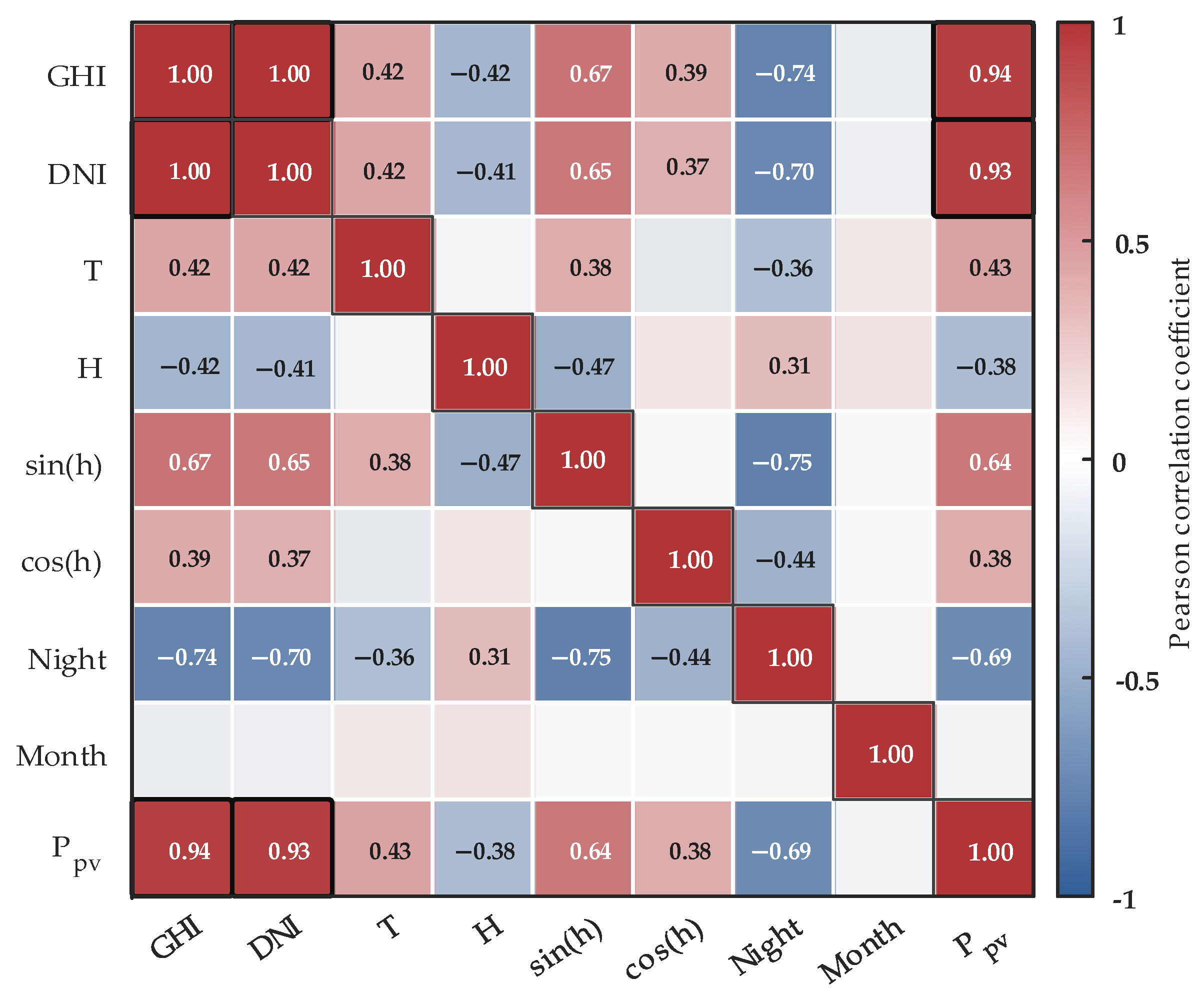
Figure 1 shows the Pearson correlation matrix of the candidate PV power characteristics. As shown in Figure 1, irradiance-related variables exhibit the strongest correlation with PV output, confirming that solar radiation is the dominant factor determining PV generation. However, global horizontal irradiance (GHI) and direct normal irradiance (DNI) are highly correlated with each other, indicating strong feature redundancy. To reduce the risk of overfitting and avoid unnecessary input dimensionality, only GHI is retained as the primary irradiance feature. Low-correlation calendar variables, such as Month, are removed because they provide limited explanatory information for short-term PV variation. In contrast, temperature and humidity are retained because they can affect PV conversion efficiency and atmospheric attenuation. In addition, sin(Hour), cos(Hour), and IsNight are introduced to describe the diurnal trajectory and distinguish daytime and nighttime operating states. IsNight is defined as a binary indicator, with IsNight = 1 for nighttime periods and IsNight = 0 for daytime periods. Therefore, the final input vector is defined as [GHI, T, H, sin(Hour), cos(Hour), IsNight], which balances physical interpretability and model compactness.

2.1.3. CNN-GRU Forecasting Model

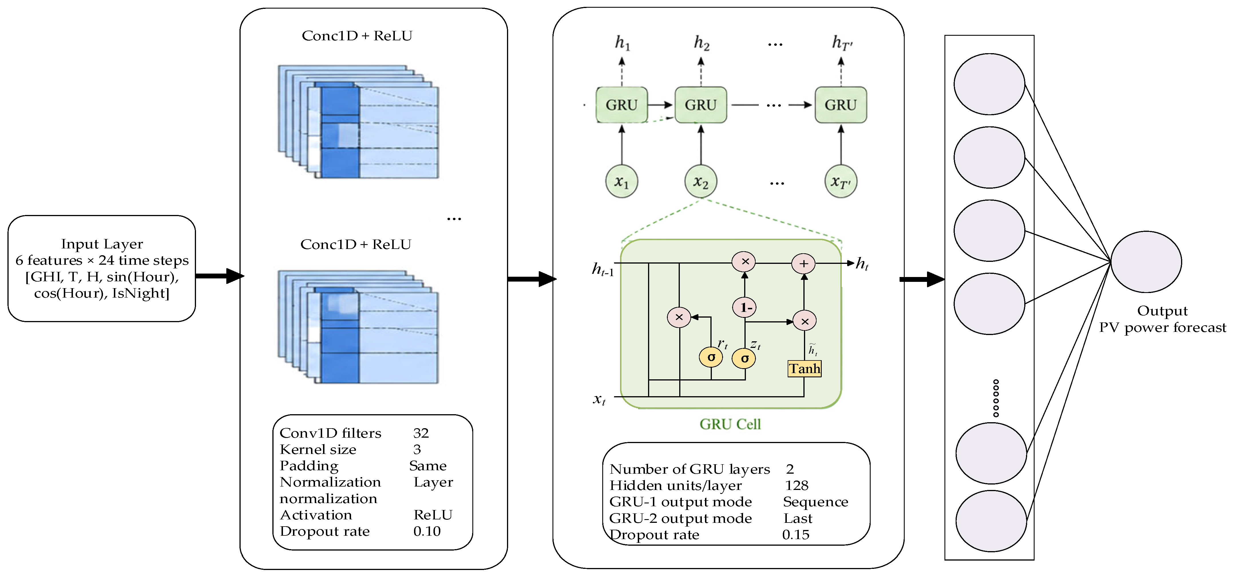
Based on the selected input features, a convolutional neural network-gated recurrent unit (CNN-GRU) forecasting model is adopted as the point forecasting engine. The reason for choosing this hybrid structure is that PV power is affected by both local meteorological patterns and sequential temporal dependencies. The one-dimensional convolutional layers are used to extract short-term local patterns from the multivariate input sequence, such as rapid changes in irradiance and weather-driven fluctuations. The gated recurrent unit (GRU) layers then model the temporal dependence of the extracted features across the forecasting window [34]. Compared with long short-term memory (LSTM), GRU has a simpler gating structure and fewer parameters, which can reduce training complexity while maintaining the ability to capture nonlinear temporal dynamics. Therefore, the CNN-GRU architecture is suitable for PV forecasting tasks where both local feature extraction and temporal memory are required.
Figure 2 illustrates the structure of the CNN-GRU forecasting model. The input layer receives a six-dimensional feature sequence over the historical time window. The convolutional module extracts local temporal features through one-dimensional convolution, normalization, Rectified Linear Unit (ReLU) activation, and dropout. The extracted feature maps are then passed to stacked GRU layers to capture sequential dependencies. Finally, a fully connected output layer maps the temporal representation to the predicted PV power.

2.1.4. Forecasting Performance Evaluation

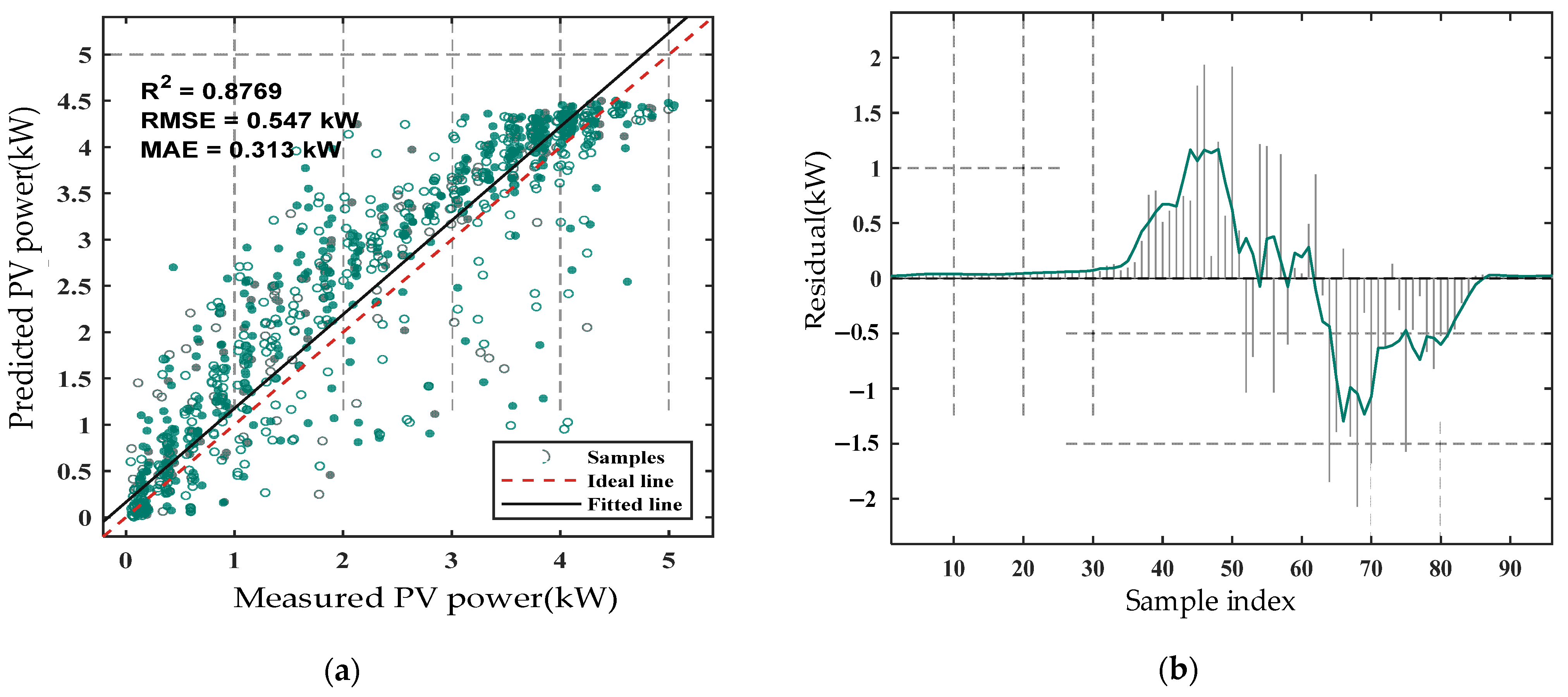
To evaluate the forecasting performance, four representative models are compared under the same training configuration: LSTM, GRU, CNN-LSTM, and CNN-GRU. LSTM and GRU are selected as recurrent neural network baselines, while CNN-LSTM and CNN-GRU are used to examine whether convolutional feature extraction can improve temporal forecasting performance. All models are trained using the Adam optimizer with an initial learning rate of 0.001, a batch size of 64, 128 recurrent hidden units, early stopping with a patience of 10 epochs, and gradient clipping with an L2-norm threshold of 1.0. The coefficient of determination (R2), root mean square error (RMSE), and mean absolute error (MAE) are used as evaluation metrics. The cross-comparison metrics for the training performance of each model are shown in Table 1.
As shown in Table 1, CNN-GRU achieves the highest R2 value of 0.8769 and the lowest RMSE of 0.547 kW among all tested models, indicating the best overall fitting accuracy and error control. Although LSTM obtains a slightly lower MAE than CNN-GRU, its RMSE is higher, suggesting that CNN-GRU performs better in suppressing larger prediction errors. This feature is important for stochastic scheduling because large PV forecast deviations can directly affect scenario generation and dispatch robustness. The comparison also shows that simply adding convolutional layers does not necessarily improve all recurrent models, as CNN-LSTM performs worse than LSTM in this case. By contrast, CNN-GRU benefits from convolutional feature extraction while maintaining a relatively compact recurrent structure. Therefore, CNN-GRU is selected as the deterministic forecasting engine for subsequent probabilistic uncertainty modeling. Therefore, CNN-GRU is selected as the deterministic forecasting engine for subsequent probabilistic uncertainty modeling. Figure 3 further shows the forecasting performance of the CNN-GRU model. The predicted PV power is generally consistent with the measured values, and the residuals are mainly distributed around zero, indicating reliable point forecasting performance and supporting the subsequent uncertainty modeling.

2.2. Uncertainty Modeling and Scenario Reduction

Although the CNN-GRU model provides accurate point forecasts, deterministic predictions alone cannot represent the uncertainty range required by risk-aware scheduling. In oilfield microgrids, PV forecast errors may affect not only grid interaction and operating cost, but also the dispatch of electric-to-thermal resources coupled with pipeline safety. Therefore, the deterministic CNN-GRU output is further extended into a probabilistic uncertainty description.

2.2.1. Quantile-Regression-Based Probabilistic Interval Construction

To characterize the conditional distribution of PV power output under different cumulative probabilities τ (τ ∈ {0.05,0.1,…,0.95}), a non-parametric quantile regression (QR) model is established [10]. Compared with assuming a fixed error distribution, quantile regression can estimate prediction intervals directly from data and is therefore suitable for renewable generation with non-Gaussian and time-varying uncertainty. For each scheduling time step t, the τ-conditional quantile of the actual PV power Pt is modeled as a linear function of the CNN-GRU point prediction P ^ t :
Q P t ( τ | P ^ t ) = a τ P ^ t + b τ
where the optimal parameter set {aτ,bτ} is determined by solving the following pinball loss minimization problem over the historical training dataset of D days:
min a τ , b τ 1 D d = 1 D ρ τ ( P d , t ( a τ P ^ d , t + b τ ) )
where Pd,t and P ^ d , t represent the measured and predicted PV power on day d, respectively; and ρτ(u) = u(τ − 1{u < 0}) is the standard asymmetric check function. By solving (3) across the quantile vector τ, the continuous conditional probability density envelope of day-ahead PV output is successfully mapped. The parameters {aτ,bτ} for each quantile level tau are obtained by minimizing the pinball loss over all historical daily profiles. Therefore, the daily power profiles are used to calibrate the conditional quantile relationship between the point forecast and the actual PV realization. These parameters are not decision variables of the scheduling model. Instead, they are forecasting-layer parameters that convert the CNN-GRU point forecast into probabilistic PV intervals, which are subsequently transformed into representative PV scenarios for the stochastic scheduling problem.

2.2.2. Gaussian-Copula-Based Temporal Dependence Modeling

Simple QR only describes the marginal distribution of PV power at each time step, failing to capture the temporal correlation of intraday power sequences. To address this limitation, this paper introduces multivariate Gaussian Copula to model the time-series dependence of PV output [35]. The specific steps are as follows:
  • Standard Normal Mapping. The historical actual PV power Pd,t is transformed into the standard normal space zd,t via the Probability Integral Transform (PIT):
z d , t = Φ 1 ( F t ( P d , t ) )
where Ft(·) is the marginal cumulative distribution function (CDF) constructed by interpolating the QR bands, and Φ−1(·) represents the inverse CDF of the standard normal distribution.
  • Covariance Modeling and Sampling. The temporal dependency of the transformed sequence Z = [zd,1,…,zd,T] is captured by calculating its chronological covariance matrix Σ R T × T . Based on the estimated covariance, Slarge correlated normal scenarios are sampled:
z ~ s N ( 0 , Σ ) , s = 1 , , S l a r g e
  • Inverse Physical Mapping. The sampled standardized trajectories zs,t are mapped back to standard uniform variables and subsequently converted into physically meaningful PV scenarios using the inverse marginal CDF:
P s , t = F t 1 ( Φ ( z ~ s , t ) )
where Ps,t is the synthesized PV output of scenario s at time step t, which inherently preserves both the deterministic forecast trend and historical temporal dependency patterns.

2.2.3. Scenario Reduction

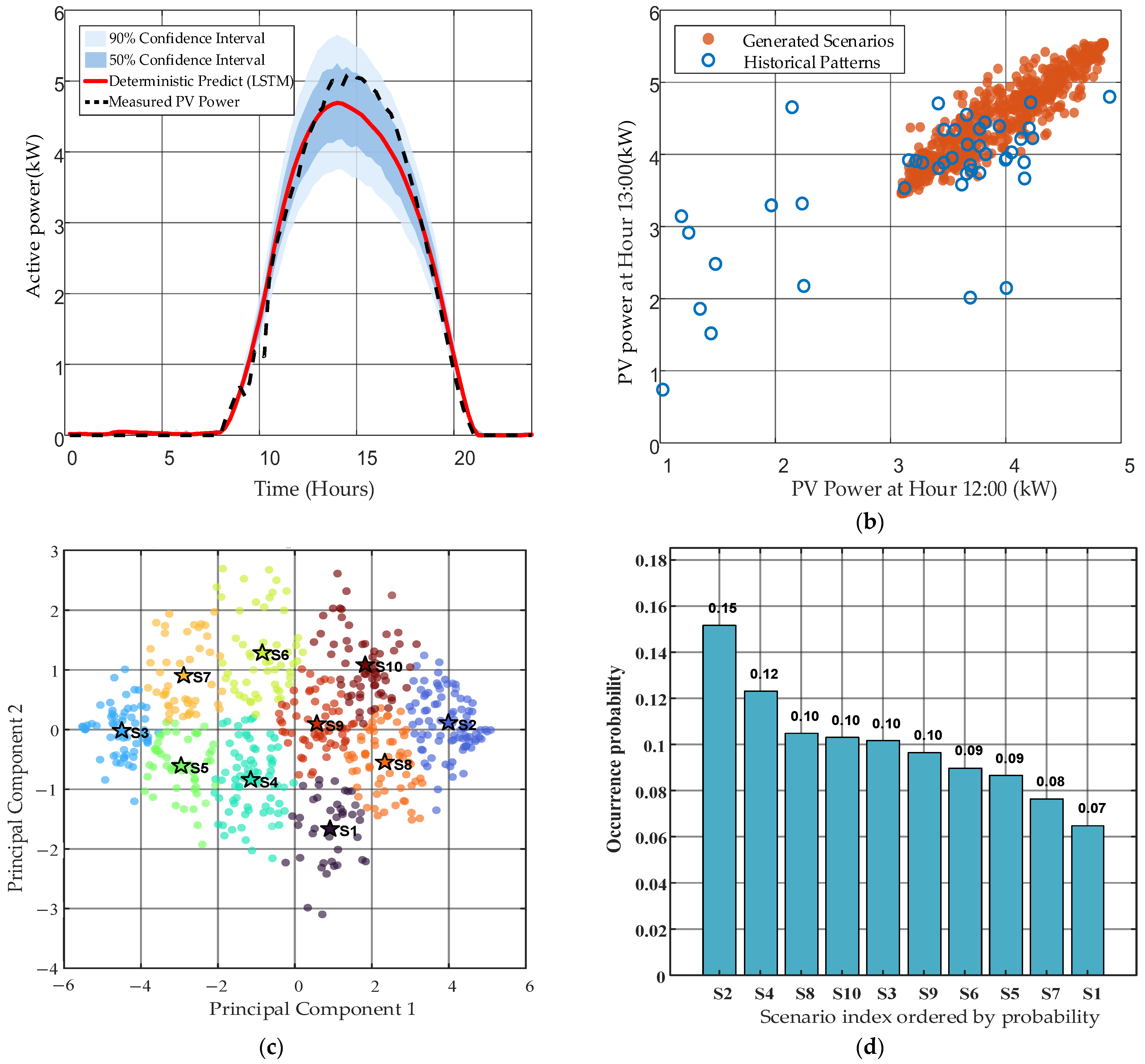
Directly using a large number of generated PV scenarios would increase the computational burden of the subsequent stochastic scheduling problem. Therefore, scenario reduction is performed to obtain a small number of representative trajectories while retaining the main uncertainty characteristics [36]. In this study, Slarge = 500 PV scenarios are first generated by the probabilistic model. Principal Component Analysis (PCA) is then applied to project the high-dimensional daily PV trajectories into a low-dimensional feature space while retaining more than 95% of the cumulative variance. K-means clustering is subsequently performed in the PCA-reduced space, and the cluster centroids are selected as representative PV scenarios. The occurrence probability of each representative scenario is calculated according to the proportion of original scenarios assigned to the corresponding cluster. Finally, S = 10 representative day-ahead PV profiles and their probabilities are obtained for stochastic scheduling.
Figure 4 presents the uncertainty modeling and scenario reduction results. Figure 4a shows that the constructed prediction intervals can cover the measured PV trajectory and provide a reasonable uncertainty envelope around the deterministic forecast. Figure 4b compares generated scenarios with historical patterns at selected time points, indicating that the Gaussian-Copula-based sampling preserves the dependence structure of PV outputs. Figure 4c shows the clustering results in the PCA-reduced space, where the generated scenarios are grouped into representative clusters. Figure 4d gives the occurrence probabilities of the selected representative scenarios. The probabilities are not uniform, indicating that the scenario set reflects the uneven likelihood of different PV fluctuation patterns. These results show that the proposed uncertainty modeling process can transform probabilistic forecasting information into a tractable scenario set for downstream stochastic optimization.
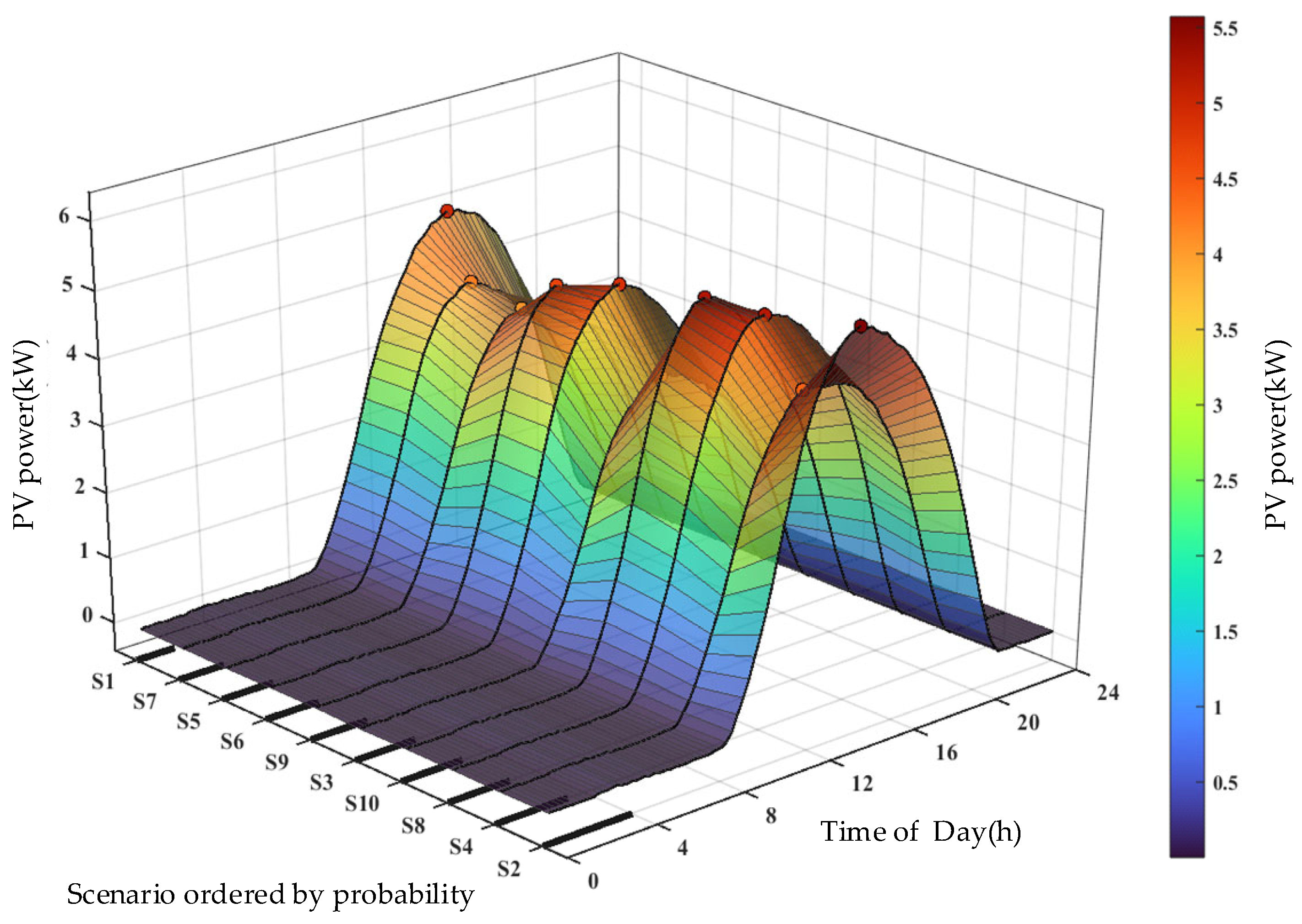
To further visualize the temporal profiles of the reduced scenario set, Figure 5 shows the representative PV trajectories ordered by occurrence probability. The selected scenarios cover different PV generation patterns, including high-output, medium-output, and low-output profiles, while preserving the typical daytime rise-and-fall structure of PV power. This confirms that the reduced scenario set retains sufficient diversity for evaluating dispatch decisions under renewable uncertainty.

3. Physics-Based Modeling of Oilfield Electric-to-Thermal Conversion and Thermo-Hydraulic Coupling

The stochastic PV scenarios generated in Section 2 provide the primary uncertainty inputs for the scheduling model. Although practical oilfield operations may also involve uncertainties from load fluctuations, equipment availability, production-plan changes, and measurement errors, this study focuses on PV uncertainty as the dominant stochastic factor in renewable-rich oilfield microgrids. This is because PV output directly affects renewable accommodation, grid interaction, and ETSB charging opportunities, while major production loads are generally operated according to predefined production plans and safety requirements at the day-ahead timescale. This assumption defines the modeling scope rather than excluding other uncertainties.
To ensure the physical executability of scheduling decisions, the impacts of production-side characteristics are represented through physics-based models and operational constraints. Specifically, pumping-unit power fluctuations, ETSB thermal dynamics, and crude-oil pipeline temperature limitations are incorporated into the scheduling framework. Therefore, this section establishes the oilfield-specific physical models that couple renewable uncertainty with production processes and provide the basis for safe and executable stochastic scheduling.

3.1. Time-Scale Transformation of Reciprocating Pumping Loads

The rigid electrical load of an oilfield mainly consists of reciprocating pumping units, gathering and transportation pump stations, and auxiliary production facilities. Among them, reciprocating pumping units usually account for a major share of electricity consumption and exhibit a typical periodic power profile during each stroke cycle [37]. If this second-level mechanical fluctuation is directly embedded into an hourly day-ahead scheduling model, the optimization dimension and computational burden would increase substantially. More importantly, such high-frequency oscillations are not directly actionable for day-ahead dispatch. Therefore, a time-scale transformation is required to preserve the energy contribution of pumping loads while making them compatible with the scheduling horizon. To simplify the mathematical representation, the instantaneous active power Pbase(t) of a pumping unit within one stroke cycle can be idealized as a piecewise sinusoidal function:
P b a s e ( t ) = P H m a x sin ( ω H λ ) , 0 λ < T H , P K m a x sin ω K ( λ T H ) , T H λ < T 0
where Pbase(t) is the active power of the pumping unit at time t, T0 and TH are the active power cycle and energy dissipation cycle of the pumping unit’s stroke, respectively, PHmax and PKmax are the peak energy-dissipating power and peak energy-supplying power of the oil pump, respectively, ωH and ωK are the angular frequencies of the energy-dissipating phase and energy-supplying phase of the oil pump, respectively. λ = tkT0, representing the instantaneous time during the k-th cycle of the pumping unit, is used solely to simplify the mathematical expression.
For day-ahead energy management, the scheduling model does not need to track the second-level oscillatory trajectory of each pumping unit. Instead, the cyclic power profile is converted into an equivalent average power over one stroke cycle. Consequently, an Integral-Average Transformation is implemented to derive the equivalent mean power Pbase,avg over a scheduling horizon:
P b a s e , a v g = 2 π · T 0 P H m a x · T H + P K m a x · ( T 0 T H )
This transformation preserves the energy-equivalent contribution of the cyclic pumping process while avoiding the direct introduction of high-frequency mechanical dynamics into the hourly optimization problem. Based on the equivalent power of each pumping-unit type, the aggregated rigid baseload of the oilfield Pbase,total(t) is formulated as:
P b a s e , t o t a l ( t ) = i = 1 N p u m p N i ( t ) P b a s e , a v g , i + P o t h e r ( t )
where Npump represents the classification of different models within the pump group, Ni(t) is the activation status of the i-th class of pumping units, and Pother(t) accounts for fixed auxiliary electrical demands. Through this time-scale transformation, the rigid production load is represented by a scheduling-compatible electrical demand profile, which provides the baseline load for the subsequent PV absorption and ETSB dispatch model. The pumping-unit parameters used in this study are listed in Appendix Table A1.

3.2. ETSB Electric-to-Thermal Conversion and Pipeline Thermo-Hydraulic Coupling

After the rigid electrical load is determined, the remaining dispatchable flexibility mainly comes from the ETSB-based electric-to-thermal conversion process. Unlike ordinary electrical storage or building heating loads, the ETSB in an oilfield is directly connected with crude-oil gathering and transportation safety. Its charging power affects the thermal storage state, while its heat release determines whether the pipeline fluid temperature can be maintained above the paraffin-waxing threshold. Therefore, the ETSB must be modeled together with heat exchange and pipeline temperature evolution.
This subsection establishes a coupled electric-thermal-hydraulic model for the ETSB and the crude-oil pipeline. The model links the dispatch variable Peb,act,s(t) with the thermal storage state Sth,s(t), boiler temperature Tboiler,s(t), heat supplied to the pipeline Qd,s(t), and pipeline fluid temperature Tpipe,s(t). This coupling makes it possible to evaluate whether a candidate dispatch command is not only electrically beneficial, but also physically feasible for crude-oil transportation. For details on the parameters discussed in this section, see Table A1 in the Appendix.

3.2.1. Thermal Storage State Dynamics of the ETSB

The ETSB stores electrical energy in the form of heat and releases thermal energy to the pipeline heating loop when required. Considering electro-thermal conversion efficiency, self-dissipation, standby heat loss, and heat extraction for pipeline heating, the SOC evolution of the ETSB under scenario s is described as:
S t h , s ( t + 1 ) = ( 1 γ l o s s Δ t ) S t h , s ( t ) + η e b P e b , a c t , s ( t ) Δ t Q d , s ( t ) Δ t Q l o s s Δ t Q c a p
where Sth,s(t) represents the SOC of the thermal storage under scenario s at time t, γloss is the self-discharge coefficient, ηeb is the electro-thermal conversion efficiency, Peb,act,s(t) denotes the actual power consumption of the ETSB, Qcap is the rated thermal capacity, and Qd,s(t) is the thermal load extracted for pipeline heating, Q l o s s represents the standby thermal dissipation rate, and Δt is the discrete time interval for the scheduling horizon. The SOC is further mapped to the boiler-side thermal state through a linear temperature relationship:
T b o i l e r , s ( t ) = S t h , s ( t ) ( T m a x T m i n ) + T m i n
where Tmax and Tmin are the upper and lower operating temperature limits of the ETSB. Equations (10) and (11) describe the available thermal energy and heat-exchange potential of the ETSB. Therefore, they provide the physical basis for determining whether the ETSB can absorb surplus PV power or supply sufficient heat to the pipeline at each scheduling period.

3.2.2. Heat Exchange and Pipeline Temperature Regulation

The heat supplied by the ETSB must compensate for pipeline heat loss and maintain the crude-oil fluid temperature within the safe operating range. The pipeline heat loss under scenario s is expressed as:
Q p i p e _ l o s s , s ( t ) = K p i p e T p i p e , s ( t ) T s o i l
where Kpipe is the pipeline insulation coefficient and Tsoil is the surrounding soil temperature at the pipeline burial depth. Based on the current pipeline temperature and the target operating temperature, the ideal heat demand is calculated as:
Q d e m a n d , s ( t ) = Q p i p e _ l o s s , s ( t ) + K g a i n T t a r g e t T p i p e , s ( t )
where Kgain is the feedback gain of the temperature regulation process and Ttarget is the desired pipeline temperature. However, the actual heat delivered to the pipeline is also constrained by the heat-exchange capability between the ETSB and the pipeline loop. Therefore, the heat supplied to the pipeline is limited by:
Q d , s ( t ) = max 0 , min Q d e m a n d , s ( t ) , h H E X T b o i l e r , s ( t ) T w a t e r _ i n
where hHEX is the heat-exchange coefficient and Twater_in is the inlet water temperature of the pipeline heating loop. This expression ensures that the heat supplied to the pipeline does not exceed either the thermal demand or the physical heat-exchange capacity. The temporal evolution of the internal pipeline fluid temperature Tpipe,s(t) is then updated:
T p i p e , s ( t + 1 ) = T p i p e , s ( t ) + Δ t C p i p e Q d , s ( t ) Q p i p e _ l o s s , s ( t )
where Cpipe is the equivalent thermal capacity of the pipeline system. Equation (15) links the ETSB heat-supply decision to the dynamic pipeline safety state. If the ETSB dispatch is insufficient, the pipeline temperature may decrease toward the paraffin-waxing threshold; if excessive heat is supplied, the system may waste electrical energy or violate upper thermal limits. Therefore, this thermo-hydraulic model embeds crude-oil transportation safety directly into the energy scheduling process.

4. Physics-Embedded Stochastic Multi-Objective Scheduling Model

Based on the PV uncertainty scenarios generated in Section 2 and the oilfield electric–thermal–hydraulic models established in Section 3, this section formulates a stochastic multi-objective scheduling model for PV-integrated oilfield microgrids. The model coordinates grid-interaction smoothing, operating economy, PV absorption, and crude-oil pipeline safety under renewable uncertainty. Unlike conventional microgrid dispatch models that usually rely on deterministic PV forecasts and simplified electrical load descriptions, the proposed formulation embeds thermo-hydraulic safety constraints directly into the scheduling process. In this way, the ETSB is optimized not merely as a controllable electrical load, but as an electric-to-thermal flexibility resource coupled with pipeline temperature regulation.

4.1. Formulation of Multi-Objective Functions

The scheduling decision variable is the day-ahead ETSB power command, which is further corrected through the physical feasibility mechanisms described in Section 4.3. For each representative PV scenario, the actual ETSB power affects the grid interaction, PV curtailment, thermal storage state, and pipeline temperature. Therefore, three objectives are formulated to represent grid-side stability, operating economy, and renewable accommodation.
  • Minimization of expected grid-interaction variance (f1). The first objective aims to reduce the temporal fluctuation of the power exchanged between the oilfield microgrid and the external grid. A smoother grid-interaction profile can mitigate PV-induced power shocks at the point of common coupling and improve operational stability:
min f 1 = s = 1 S π s V a r P g r i d , s ( t )
where f1 is the expected net-load variance, Var(·) represents the 24-h temporal variance operator, and πs is the probability of scenario s. Pgrid,s(t) denotes the purchased power from the utility grid and is constrained to be non-negative:
P g r i d , s ( t ) = max 0 , P g r i d , r i g i d ( t ) + P e b , a c t , s ( t ) P p v , s ( t )
where Pgrid,rigid(t) represents the aggregated rigid load, Ppv,s(t) denotes the output of the PV system under scenario s.
  • Minimization of expected operational expenditure (f2). The second objective describes the expected electricity procurement cost under the time-of-use tariff. By shifting ETSB electricity consumption to periods with lower electricity prices or higher PV availability, the scheduling model can improve operating economy while maintaining thermal safety:
min f 2 = s = 1 S π s t = 1 T c ( t ) P g r i d , s ( t ) Δ t
where f2 represents the expected electricity procurement cost, and c(t) denotes the time-of-use (TOU) electricity tariff at time step t.
  • Minimization of expected PV curtailment rate (f3). The third objective aims to improve local PV absorption. In the oilfield microgrid, surplus PV power can be converted into stored heat through the ETSB, but this absorption capability is constrained by the ETSB capacity, SOC, heat-exchange ability, and pipeline temperature safety. The expected PV curtailment rate is formulated as:
min f 3 = s = 1 S π s t = 1 T P c u r t , s ( t ) t = 1 T P p v , s ( t ) + ε
P c u r t , s ( t ) = max 0 , P p v , s ( t ) P g r i d , r i g i d ( t ) + P e b , a c t , s ( t )
where f3 is the expected PV curtailment rate, Pcurt,s(t) denotes the PV power that cannot be locally absorbed at time t under scenario s, and ε is a small positive constant used to avoid numerical singularity. These three objectives are conflicting: increasing ETSB consumption may reduce PV curtailment and smooth grid interaction, but it may also increase electricity cost or push the thermal storage state toward its limits. Therefore, the scheduling problem is solved as a stochastic multi-objective optimization problem to obtain Pareto trade-offs among stability, economy, and renewable utilization.

4.2. Operational and Security Constraints

The operational constraints are imposed to ensure both electrical feasibility and production-side safety. In contrast to generic microgrid constraints, the constraints in this study explicitly include the thermo-hydraulic safety boundary of crude-oil transportation. This is essential because an ETSB schedule that appears beneficial from the grid side may be infeasible if it causes excessive SOC depletion, insufficient heat supply, or unsafe pipeline temperature. First, the Peb,act,s(t) of the ETSB is further bounded by its rated maximum capacity:
0 P e b , a c t , s t P e b , m a x ,   t , s
where Peb,max represents the rated maximum active power capacity of the ETSB.
Second, the ETSB power variation is constrained by the thermal and mechanical response capability of the electric-to-thermal system:
P e b , a c t , s ( t ) P e b , a c t , s ( t 1 ) Δ P e b , m a x , t = 1,2 . . . T , s
where ΔPeb,max denotes the maximum allowable power variation of the ETSB within a single time interval.
Third, the thermal storage SOC is restricted within safe operating limits:
S t h , s m i n S t h , s ( t ) S t h , s m a x , t , s
where [ S t h , s m i n , S t h , s m a x ] define the lower and upper SOC boundaries. Maintaining the SOC within this range avoids excessive depletion or overcharging of the thermal storage unit.
Fourth, the pipeline fluid temperature must be maintained within the allowable safety range:
T p i p e m i n T p i p e , s ( t ) T p i p e m a x , t , s
where [ T p i p e m i n , T p i p e m a x ] represents the safe temperature range to avoid crude oil solidification.
Finally, to ensure the continuity of the autonomous scheduling, the final state of the ETSB at the end of the scheduling horizon is encouraged to approach the target terminal SOC and pipeline temperature to its initial equilibrium point, facilitating “closed-loop” operation for the subsequent day:
S t h , s ( T + 1 ) S t h , s t a r g e t , T p i p e , s ( T + 1 ) T p i p e , s t a r g e t , s
where S t h , s t a r g e t and T p i p e , s t a r g e t represent the target terminal SOC of the thermal storage and the target terminal pipeline temperature, respectively. This condition prevents the optimizer from obtaining an apparently low-cost schedule by excessively consuming the thermal storage at the end of the day, thereby improving the executability of the dispatch plan for continuous daily operation. Equation (25) indicates that the terminal restoration requirement is enforced through the terminal sustainability penalty rather than as a strict equality constraint.

4.3. Oilfield-Specific Physics-Embedded NSGA-II Solver

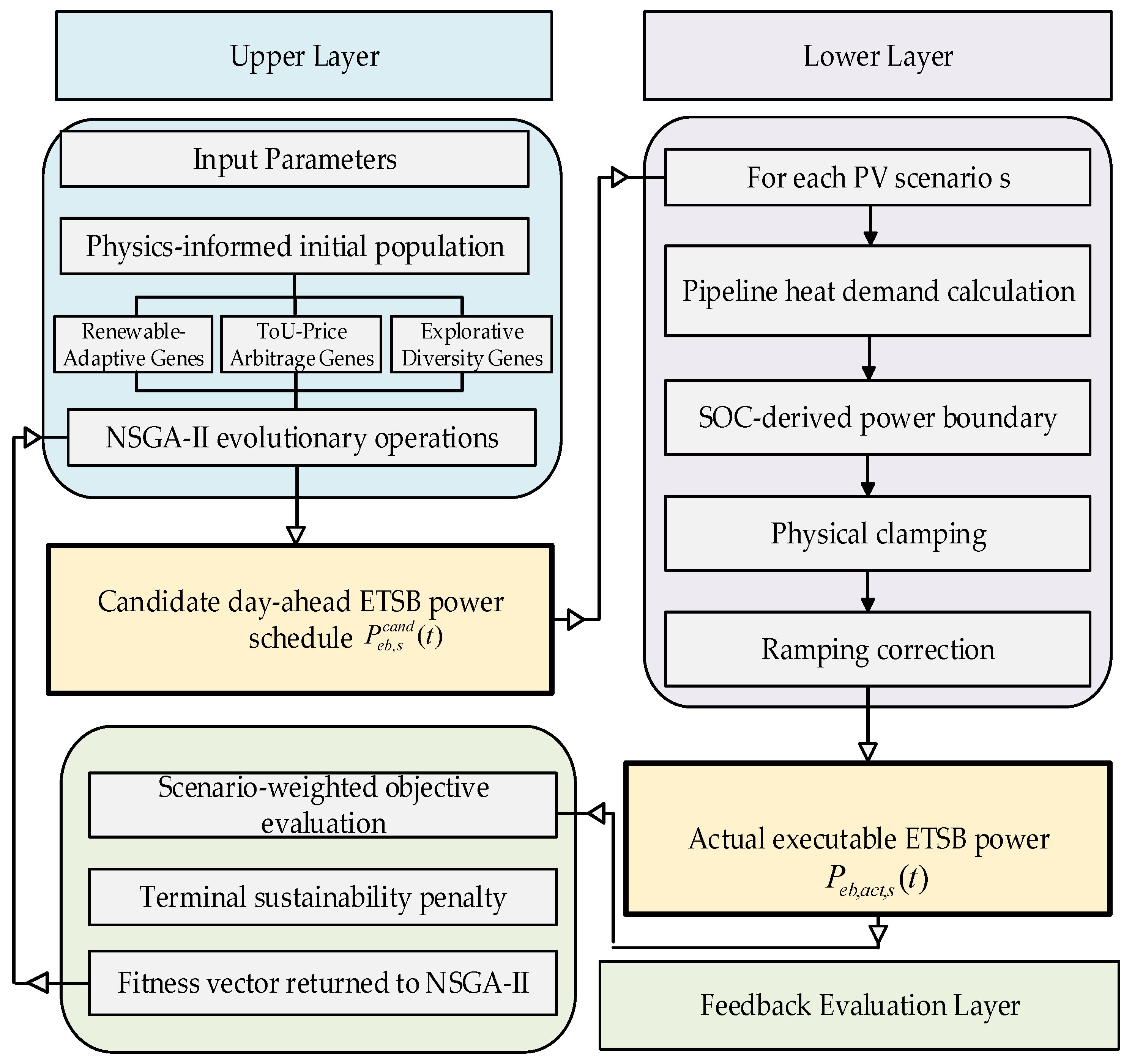
To improve feasibility, convergence, and operational executability, this study develops an oilfield-specific physics-embedded NSGA-II solver. The key idea is to embed production-side physical knowledge into the evolutionary search process rather than treating the oilfield microgrid as a black-box electrical load. As shown in Figure 6, the proposed solver consists of an upper evolutionary search layer, a lower physical correction and simulation layer, and a feedback evaluation layer. The upper layer generates candidate day-ahead ETSB power schedules. The lower layer evaluates each candidate under representative PV scenarios, calculates heat demand, derives SOC-based feasible power boundaries, applies physical clamping, and corrects ramping violations. The feedback layer then computes scenario-weighted objectives and terminal sustainability penalties before returning the fitness vector to NSGA-II.

4.3.1. Physics-Informed Population Initialization

Standard NSGA-II usually initializes individuals randomly, which may be inefficient when many randomly generated ETSB schedules violate thermal storage or pipeline safety requirements. To guide the initial population toward physically meaningful regions, a domain-knowledge-guided initialization strategy is adopted. The initial population with Npop = 120 is divided into three groups with a 1:1:1 ratio.
The first group is the renewable-adaptive gene group. For time periods with relatively high PV output, the ETSB power is initialized according to the PV envelope so that the initial schedules have the ability to absorb surplus renewable energy.
The second group is the time-of-use price arbitrage gene group, in which higher ETSB charging levels are assigned to valley-price periods to improve economic performance.
The third group is the explorative diversity gene group, where stochastic perturbations are introduced to preserve population diversity and avoid premature convergence. Through this initialization strategy, the initial population covers renewable accommodation, economic operation, and exploratory search directions, which improves the search efficiency of the subsequent evolutionary process.

4.3.2. Bilevel Search-Simulation Architecture

The proposed scheduling problem contains two different layers of complexity. The evolutionary algorithm searches for a 24-h day-ahead ETSB power trajectory, while the feasibility of this trajectory depends on recursive thermo-hydraulic state transitions under multiple PV scenarios. Directly encoding all SOC and pipeline temperature states as decision variables would significantly increase the dimensionality of the optimization problem. Therefore, a bilevel search-simulation architecture is constructed.
In the upper layer, NSGA-II evolves the candidate ETSB power schedule. In the lower layer, a forward physical simulation engine updates the SOC, boiler temperature, heat exchange, and pipeline temperature for each PV scenario. This design keeps the decision space compact while retaining the physical fidelity of the oilfield electric–thermal–hydraulic process. As a result, the optimizer searches over actionable dispatch commands, while the state variables are generated through physical simulation rather than treated as independent decision variables.

4.3.3. Self-Coupling Correction and Physical Clamping

During the evolutionary search, a candidate ETSB power command may violate the SOC-derived feasible region. Instead of only penalizing such infeasible individuals after evaluation, this study introduces a backward-mapping correction mechanism. For each scenario and time step, the feasible lower and upper bounds of the ETSB power are derived from the SOC state equation:
P e b _ m i n , s ( t ) = S t h , s m i n ( 1 γ l o s s Δ t ) S t h , s ( t ) Δ t Q c a p + Q d , s ( t ) + Q l o s s / η e b
P e b _ m a x , s ( t ) = S t h , s m a x ( 1 γ l o s s Δ t ) S t h , s ( t ) Δ t Q c a p + Q d , s ( t ) + Q l o s s / η e b
where Peb,min,s(t) and Peb,max,s(t) are the SOC-derived lower and upper feasible power boundaries. These boundaries represent the minimum and maximum ETSB power that can be executed without violating the SOC limits after considering heat extraction and standby heat loss.
The candidate power command generated by NSGA-II is then projected onto the feasible interval:
P e b , a c t , s ( t ) = Π [ P e b _ m i n , s ( t ) , P e b _ m a x , s ( t ) ] P e b , s c a n d ( t )
Π [ a , b ] ( x ) = min b , max { a , x }
where P e b , s c a n d represents the candidate power command generated by the NSGA-II under scenario s, Π[a, b] (·) denotes the projection operator onto the closed interval [a, b]. If the candidate ETSB power lies within the feasible range, it is retained; otherwise, it is clipped to the nearest admissible boundary. This physical clamping mechanism reduces infeasible individuals before the thermo-hydraulic forward simulation, thereby improving both computational efficiency and practical executability.

4.3.4. Temporal Dynamic Ramping Filter

Even if the SOC constraints are satisfied, the ETSB power trajectory may still contain abrupt changes that exceed the allowable ramping capability. Such commands are difficult to execute in practical oilfield operation and may also cause unnecessary thermal stress. Therefore, a temporal dynamic ramping filter is applied after physical clamping to sequentially correct the ETSB power trajectory:
P e b , a c t , s ( t ) = max P e b , a c t , s ( t 1 ) Δ P e b m a x , min P e b , a c t , s ( t ) , P e b , a c t , s ( t 1 ) + Δ P e b m a x
This filter ensures that the actual ETSB power at each time step remains within the upward and downward ramping limits determined by the previous executable power. Therefore, the generated schedule is not only feasible in terms of SOC, but also consistent with the dynamic response capability of the electric-to-thermal system.

4.3.5. Terminal Sustainability Penalty

To ensure inter-temporal operational continuity, a Sustainability Penalty Function Ψterm using the ReLU activation structure is integrated into the fitness evaluation. For any scenario s, the terminal deviations of SOC and pipeline temperature are quantified:
Δ S t h , s t e m = max 0 , S t h , s t a r g e t S t h , s ( T + 1 ) ε s
Δ T p i p e , s t e m = max 0 , T p i p e , s t a r g e t T p i p e , s ( T + 1 ) ε t
where Δ S t h , s t e m and Δ T p i p e , s t e m denote the terminal SOC deviation and terminal pipeline-temperature deviation under scenario s, respectively, ε s and ε t are allowable tolerance thresholds for terminal SOC and pipeline-temperature restoration, respectively. The terminal sustainability penalty is calculated as the scenario-weighted expectation over all representative PV scenarios:
Ψ t e r m = s = 1 S π s λ 1 Δ S t h , s t e m + λ 2 Δ T p i p e , s t e m
where λ1, λ2 are penalty coefficients for terminal SOC deviation and terminal pipeline-temperature deviation, respectively. Since the three objectives have different physical units and numerical magnitudes, each objective is first normalized before being integrated with the terminal penalty:
f ~ i = f i f i m i n f i m a x f i m i n + ε , i = 1,2 , 3
where f i m i n and f i m a x denote the minimum and maximum values of the i-th objective in the current population, respectively, and ε is a small positive constant used to avoid numerical singularity. The final fitness vector used in the improved NSGA-II is then formulated as:
F o p t = f ~ 1 + β 1 Ψ t e r m , f ~ 2 + β 2 Ψ t e r m , f ~ 3 + β 3 Ψ t e r m T
where β1, β2, and β3 are penalty weighting factors. By embedding the terminal sustainability penalty into the normalized objective vector, the solver can distinguish physically sustainable schedules from solutions that are numerically attractive but unsuitable for continuous oilfield operation.

5. Results Analysis

To evaluate the effectiveness and practical applicability of the proposed physics-embedded stochastic scheduling framework, simulations are conducted on a typical PV-integrated oilfield microgrid. The evaluation is organized from three perspectives. First, the stochastic multi-objective optimization results are analyzed to clarify the trade-off among grid-interaction smoothing, operating cost, and PV absorption. Second, deterministic and stochastic scheduling schemes are compared under the same PV uncertainty scenarios to examine whether scenario-based optimization improves out-of-sample robustness. Third, sensitivity analyses are performed to investigate the influence of PV penetration and initial ETSB thermal SOC on system performance.
The scheduling horizon is set to 24 h with a time interval of 0.25 h, resulting in 96 scheduling intervals. PV uncertainty is represented by 10 representative daily scenarios generated in Section 2. Unless otherwise specified, the baseline configuration adopts a PV penetration level of 90% and an initial ETSB thermal SOC of Sth(0) = 0.5. The main model and solver parameters are listed in Appendix Table A2.

5.1. Stochastic Optimization Performance

This subsection analyzes the scheduling results under the baseline configuration.

5.1.1. Computational Efficiency and Convergence Analysis

To further evaluate the computational practicality of the proposed physics-embedded NSGA-II, the computational environment and solver settings are summarized in Table 2.
As shown in Table 2, the proposed method required 8.4953 s to complete one full stochastic day-ahead optimization run, corresponding to an average computational time of 0.0850 s per generation. Although the proposed algorithm embeds additional thermo-hydraulic forward simulation, physical clamping, ramping correction, and terminal sustainability evaluation into the NSGA-II search process, the overall runtime remains low. Since the day-ahead scheduling task is solved offline before real-time operation, this computational burden is acceptable for practical oilfield microgrid energy management.
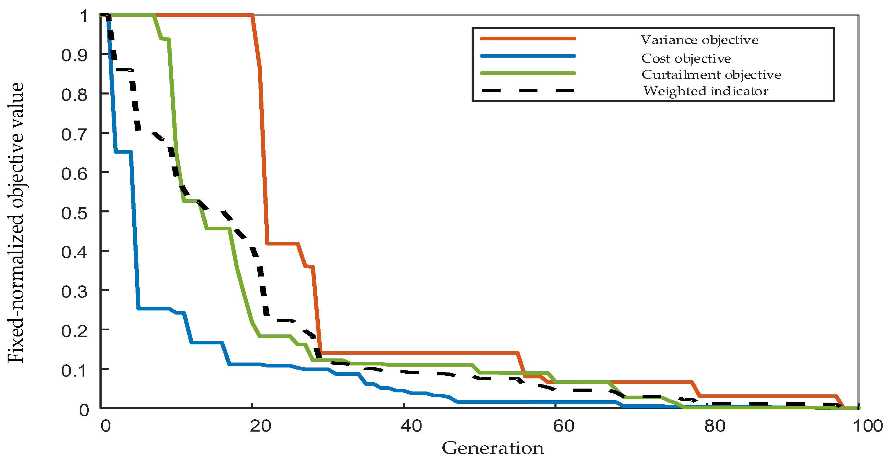
Figure 7 shows the convergence characteristics of the proposed physics-embedded NSGA-II based on fixed-normalized objective values. The fixed-normalized values are calculated using fixed reference ranges so that objectives with different units can be compared on the same scale. The weighted compromise indicator is used only to visualize the overall convergence trend and does not replace the Pareto dominance relationship. The cost objective decreases rapidly during the early generations, indicating that the solver can quickly identify lower-cost dispatch patterns. The curtailment objective also decreases progressively, reflecting the improved utilization of ETSB flexibility for absorbing surplus PV power. The variance objective presents a delayed but significant drop after approximately 20 generations, suggesting that grid-interaction smoothing requires coordinated adjustment among PV uncertainty, thermal storage states, and ramping constraints. After about 60 generations, all three objective values and the weighted compromise indicator approach stable low levels, demonstrating that the proposed solver can achieve stable convergence within the preset 100 generations.

5.1.2. Pareto Front and Compromise-Solution Selection

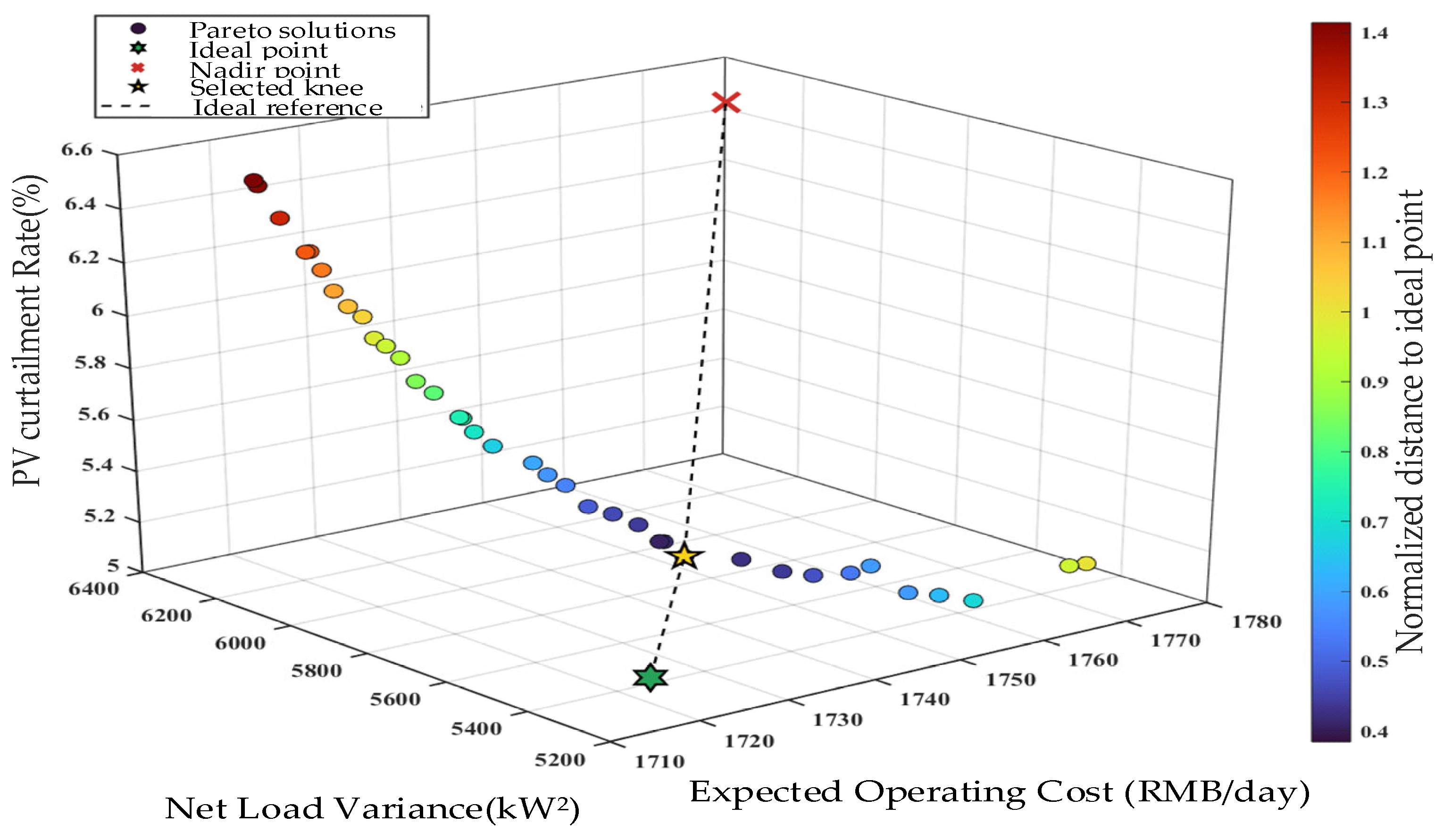
The proposed physics-embedded NSGA-II solver is first used to obtain the Pareto front of the stochastic multi-objective scheduling problem. The three objectives correspond to expected operating cost, expected net-load variance, and expected PV curtailment rate. Since these objectives are conflicting, the Pareto front is used to identify the trade-off relationship rather than a single universally optimal solution.
Figure 8 shows the three-dimensional Pareto front obtained under the baseline case. The non-dominated solutions reveal an evident trade-off among economy, grid-side smoothing, and PV absorption. When the expected operating cost decreases, the PV curtailment rate and net-load variance tend to increase, indicating that excessively cost-oriented dispatch may reduce renewable absorption and weaken grid-interaction smoothing. In contrast, solutions with lower curtailment and lower variance generally require more ETSB operation, which increases electricity procurement cost under the time-of-use tariff.
For the following dynamic analysis, a compromise solution is selected from the knee region of the Pareto front. This selection does not imply that the knee point is optimal for all operating preferences. Instead, it provides a balanced solution for illustrating how the proposed framework coordinates cost, PV absorption, and grid stability under thermo-hydraulic constraints.

5.1.3. Active Power Balance Under the Selected Solution

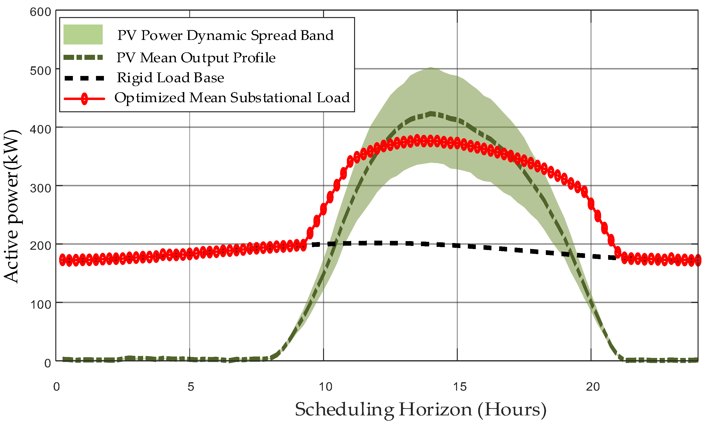
After selecting the compromise solution, the expected active power balance is analyzed to clarify how ETSB-based electric-to-thermal flexibility participates in PV absorption. Figure 9 shows the PV uncertainty envelope, the mean PV output, the rigid oilfield load, and the optimized mean substation load.
As shown in Figure 9, the rigid oilfield load remains relatively stable compared with the PV output, while PV generation mainly appears during the daytime period. Without flexible electric-to-thermal conversion, part of the midday PV output would exceed the instantaneous absorption capability of the rigid load. Under the optimized schedule, the ETSB increases electricity consumption during the PV-abundant period, thereby converting part of the renewable electricity into stored thermal energy. This behavior raises the controllable load during high-PV hours and reduces the mismatch between PV generation and oilfield demand.
The result indicates that the ETSB provides a useful demand-side flexibility resource for PV absorption. However, its dispatch is not simply to maximize electricity consumption during daytime; it is jointly constrained by the thermal SOC, heat-exchange capability, ramping limit, and pipeline temperature safety modeled in Section 3 and Section 4.

5.1.4. Thermal State Evolution and Pipeline Safety

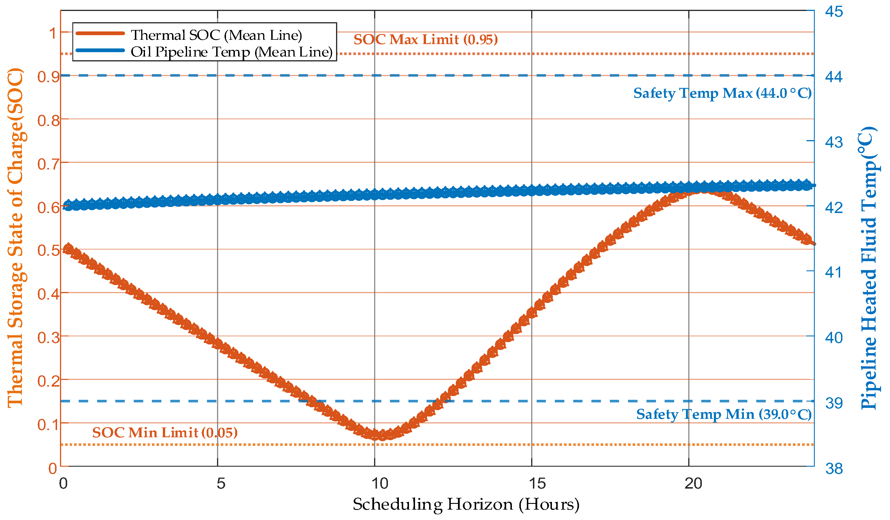
The thermo-hydraulic feasibility of the selected dispatch solution is further evaluated by tracking the ETSB thermal SOC and the pipeline fluid temperature. This analysis is necessary because a schedule that improves PV absorption may still be unacceptable if it violates thermal storage limits or reduces the pipeline temperature below the anti-wax safety threshold.
Figure 10 presents the joint evolution of the ETSB thermal SOC and pipeline fluid temperature. The SOC changes significantly over the scheduling horizon, reflecting the charging and discharging behavior of the ETSB when absorbing PV electricity and supplying heat to the pipeline. Meanwhile, the pipeline fluid temperature remains within approximately 42.0–42.3 °C, which is above the paraffin-waxing threshold of 39.0 °C and below the upper safety limit. This result shows that the selected schedule can utilize thermal storage flexibility while maintaining the required crude-oil transportation temperature.
It should be noted that the relatively narrow temperature range is obtained under the parameter settings of the studied case. Therefore, the result demonstrates feasibility for the investigated oilfield microgrid configuration, while field deployment would still require calibration using site-specific pipeline parameters and operating conditions.

5.2. Comparison with Benchmark Optimization Algorithms

To evaluate the effectiveness of the proposed physics-embedded NSGA-II, it was compared with three representative multi-objective optimization algorithms: standard NSGA-II, Multi-objective Evolutionary Algorithm Based on Decomposition (MOEA/D), and Strength Pareto Evolutionary Algorithm 2 (SPEA2) (SPEA2). MOEA/D decomposes a multi-objective optimization problem into a set of scalar subproblems and solves them collaboratively, whereas SPEA2 uses an external archive, strength-based fitness assignment, and density estimation to preserve non-dominated solutions [38,39]. All algorithms were tested under the same stochastic PV scenario set, system parameters, population size, and maximum generation number. For each algorithm, 20 independent runs were conducted with different random seeds.
The obtained solutions were evaluated using two Pareto-front quality indicators, namely hypervolume (HV) and spacing, as well as five engineering metrics: operating cost, net-load variance, PV curtailment rate, physical feasibility rate, and runtime. HV measures the convergence and coverage of the obtained Pareto front, and a larger HV value indicates better overall Pareto-front quality [40]. Spacing evaluates the distribution uniformity of non-dominated solutions, and a smaller spacing value indicates a more even solution distribution [41].
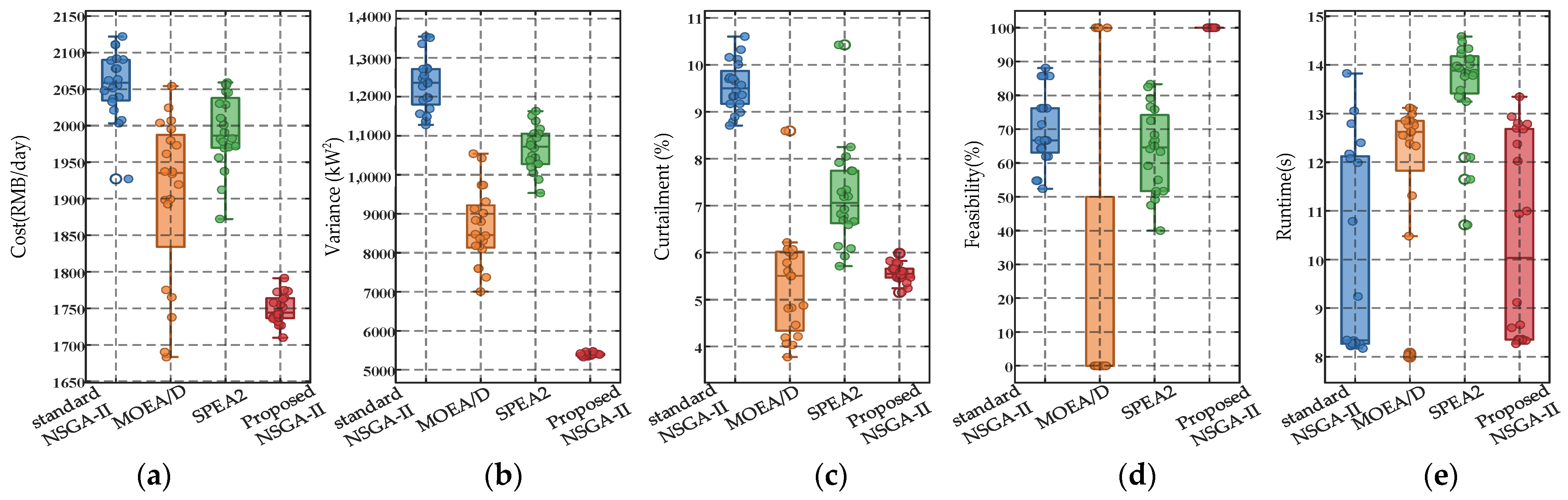
As shown in Table 3, the proposed NSGA-II achieves the largest HV value of 1.0855, which is higher than those of standard NSGA-II, MOEA/D, and SPEA2. This indicates that the proposed method obtains a Pareto front with better convergence and broader objective-space coverage. In terms of Spacing, SPEA2 achieves the smallest value, while the proposed NSGA-II obtains the second-best result. This suggests that although SPEA2 provides a slightly more uniform solution distribution, the proposed algorithm achieves better overall Pareto-front quality.
In the engineering comparison, the physical feasibility rate evaluates whether algorithm-generated schedules can be executed under oilfield thermo-hydraulic constraints. A solution is considered feasible only when all operational and thermo-hydraulic constraints are satisfied across representative PV scenarios. Figure 11 further compares the engineering performance distributions over 20 independent runs. The proposed NSGA-II achieves the lowest operating cost and the lowest net-load variance, showing stronger economic performance and grid-interaction smoothing capability. Although MOEA/D obtains a slightly lower PV curtailment rate in some runs, its physical feasibility is substantially lower and less stable. In contrast, the proposed NSGA-II maintains a 100% feasibility rate in all runs, indicating that its schedules satisfy ETSB limits, ramping constraints, SOC boundaries, and pipeline temperature safety requirements. The runtime of the proposed method remains close to standard NSGA-II and lower than SPEA2, demonstrating acceptable computational efficiency. Therefore, the observed improvements are not isolated outcomes of a single optimization trial, but consistent advantages obtained under stochastic algorithmic conditions.

5.3. Robustness Comparison Between Deterministic and Stochastic Dispatch

To examine the value of explicitly considering PV uncertainty, a deterministic scheduling scheme is introduced as a benchmark. In the deterministic scheme, the ETSB day-ahead schedule is optimized using only the nominal PV profile. In the stochastic scheme, the schedule is optimized using the representative PV scenarios and their occurrence probabilities. Both optimized schemes are then evaluated under the same 10 PV scenarios to compare their out-of-sample performance. A base case without ETSB is also included to quantify the benefit of introducing electric-to-thermal flexibility. The comparison focuses on three metrics: expected operating cost, net-load variance, and PV absorption rate. The quantitative index results of different scheduling strategies are listed in Table 4 for intuitive comparison.
As shown in Table 4, both deterministic and stochastic scheduling improve PV absorption and reduce net-load variance compared with their corresponding base cases. This confirms that ETSB-based electric-to-thermal conversion can provide effective flexibility for the studied oilfield microgrid. The deterministic optimized scheme increases the PV absorption rate from 76.28% to 95.82% and reduces net-load variance by 30.45%. The stochastic optimized scheme increases the PV absorption rate from 76.84% to 94.42% and reduces net-load variance by 56.82%. The stochastic scheme achieves a larger reduction in net-load variance, indicating that scenario-based optimization provides more conservative regulation margins for PV fluctuation. Its expected operating cost is higher than that of the deterministic optimized scheme, which reflects the cost of reserving flexibility under uncertainty. Therefore, the stochastic scheme is not simply lower-cost; rather, it provides a different trade-off by improving grid-interaction robustness and renewable accommodation reliability under uncertain PV output.
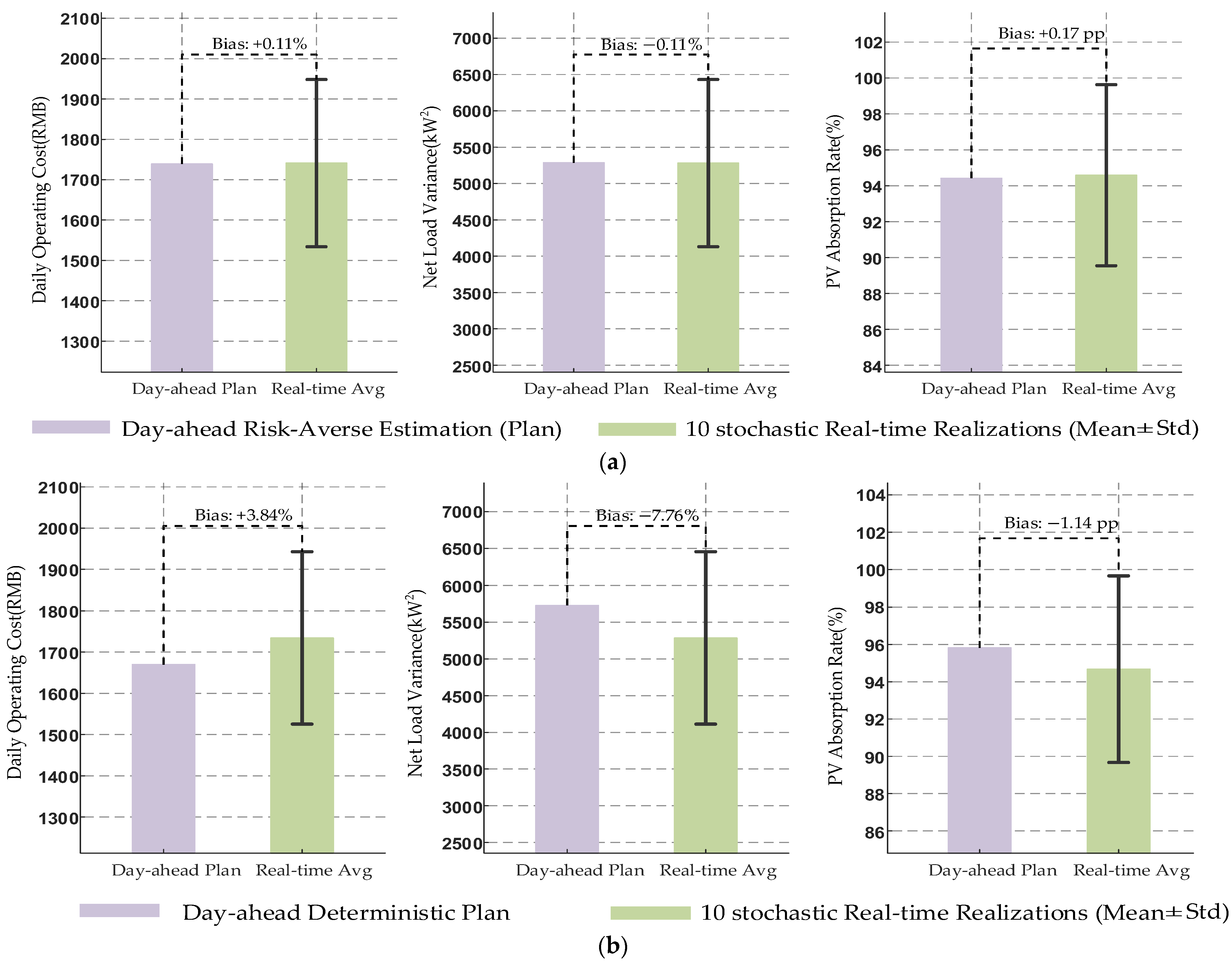
The day-ahead-to-real-time deviation is further analyzed to evaluate whether the optimized schedules remain consistent when tested under PV uncertainty. Figure 12 compares the day-ahead planned values with the real-time average values over the 10 stochastic scenarios, where the error bars represent the standard deviation across scenarios.
As shown in Figure 12, the stochastic scheme exhibits smaller deviations between day-ahead estimation and real-time scenario evaluation. Its cost deviation is approximately +0.11%, the net-load variance deviation is approximately −0.11%, and the PV absorption deviation is approximately +0.17 percentage points. In contrast, the deterministic scheme shows larger deviations because the optimized schedule is based on a single nominal PV profile and is therefore more sensitive to PV forecast errors. These results indicate that stochastic scheduling improves the consistency between day-ahead planning and scenario-based real-time evaluation in the studied case.
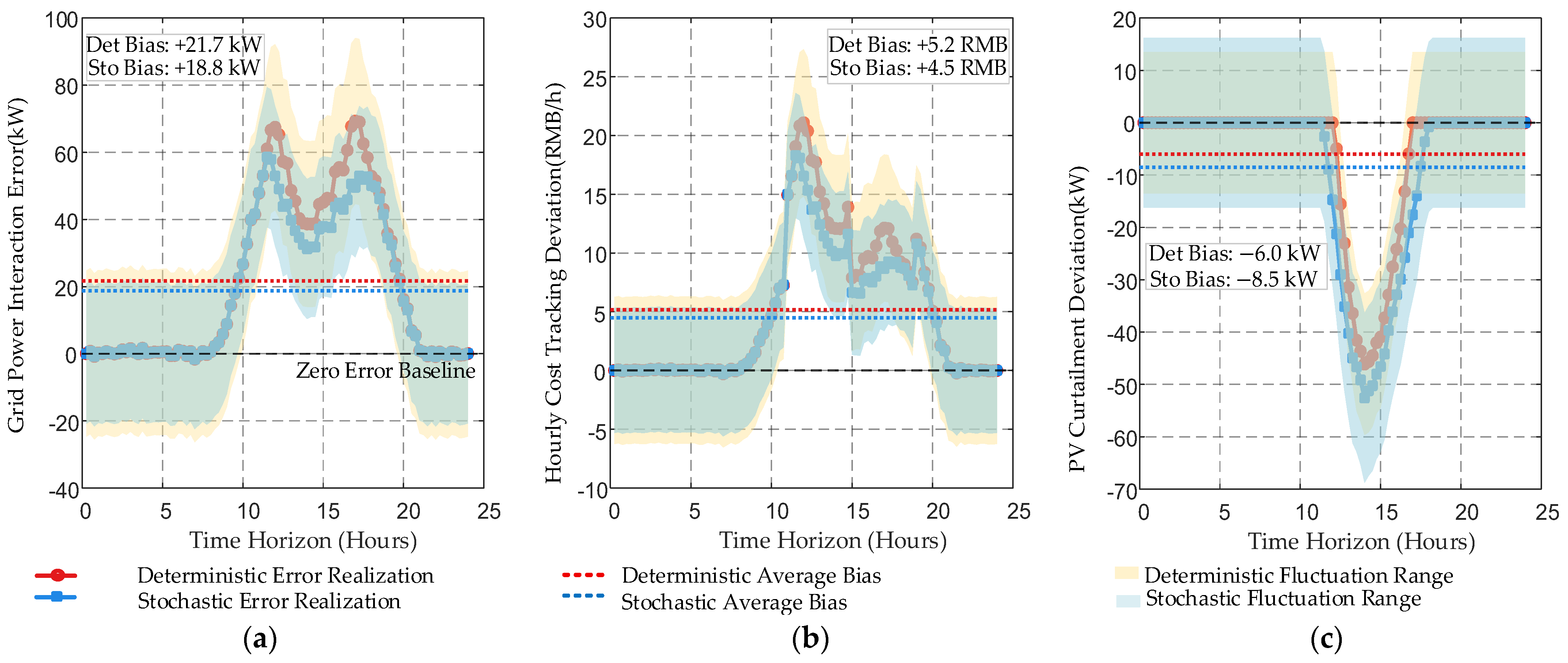
To further examine the temporal characteristics of the deviations, the worst PV fluctuation scenario is selected for hourly tracking-error analysis. Figure 13 compares the deterministic and stochastic schemes in terms of grid-interaction error, operating-cost deviation, and PV curtailment deviation.
As shown in Figure 13a,b, the deterministic scheme produces larger grid-interaction and cost deviations during the daytime PV fluctuation period, especially between 10:00 and 18:00. This is because its ETSB schedule is optimized for the nominal PV trajectory and has limited ability to accommodate deviations from that trajectory. The stochastic scheme shows smaller error bands in the same period, indicating that scenario-based optimization reserves more flexible capacity for uncertain PV changes. Figure 13c shows that the stochastic scheme can reduce curtailment deviation during periods of PV surplus by increasing ETSB electricity consumption within the feasible thermal range. This result supports the role of ETSB thermal storage as a buffer for uncertain renewable generation, while the actual effectiveness remains dependent on ETSB capacity and pipeline heat demand.

5.4. Parametric Sensitivity and Operational Boundary Investigation

Sensitivity analysis is conducted to examine how the proposed scheduling framework performs under different renewable penetration levels and different initial ETSB thermal states. The purpose is to identify operating conditions under which ETSB flexibility is more valuable and to provide practical guidance for field operators. Two parameters are considered: the PV penetration level βpv and the initial thermal SOC Sth(0).

5.4.1. Performance Under Different PV Penetration Levels

To evaluate the adaptability of the scheduling framework under different renewable development stages, three PV penetration levels are tested: 50%, 90%, and 130%. For each penetration level, deterministic and stochastic scheduling schemes are evaluated using the same performance metrics. Table 5 reports the improvement rates after ETSB integration.
As shown in Table 5, the benefit of ETSB flexibility varies with PV penetration. At 50% PV penetration, the PV absorption improvement is limited because surplus PV energy is relatively insufficient, and ETSB operation mainly relies on grid electricity for thermal charging. As PV penetration increases to 90% and 130%, more daytime renewable energy becomes available for electric-to-thermal conversion, and the ETSB becomes more useful for both PV absorption and grid-interaction smoothing. At 130% PV penetration, the stochastic scheme achieves a 47.71% reduction in net-load variance, while the deterministic scheme achieves 22.61%. This indicates that uncertainty-aware scheduling becomes more valuable when PV output is high and more volatile. However, the results should be interpreted within the studied parameter setting, especially the assumed ETSB capacity, pipeline heat demand, and PV scenario distribution.

5.4.2. Sensitivity to Initial ETSB Thermal SOC

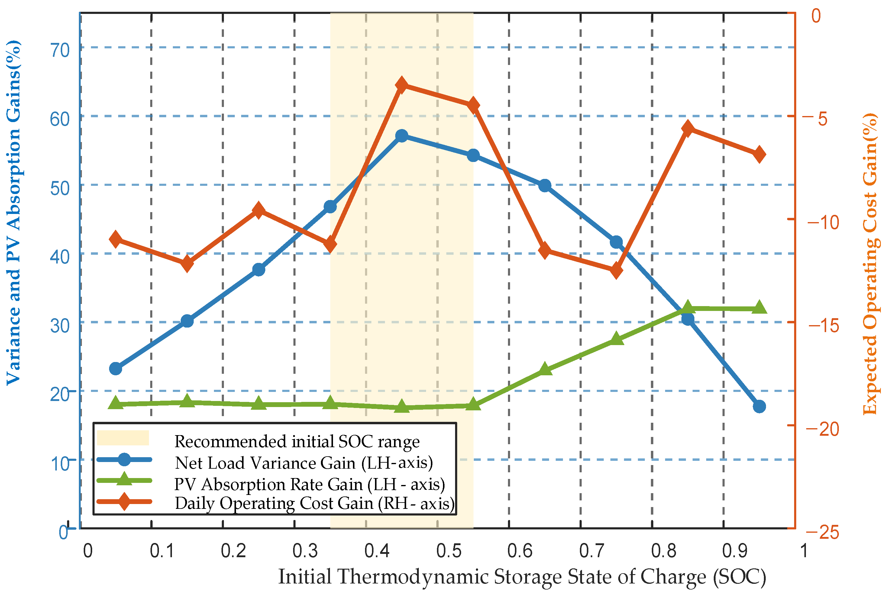
The initial thermal SOC determines both the available heat reserve and the remaining storage capacity of the ETSB. If the initial SOC is too low, the system may need to charge early to maintain pipeline thermal safety. If the initial SOC is too high, the storage headroom for absorbing midday PV surplus becomes limited. Therefore, the initial SOC is swept from 0.05 to 0.95 with a step size of 0.1 under the baseline 90% PV penetration level.
Figure 14 shows the changes in net-load variance gain, PV absorption gain, and operating-cost gain under different initial SOC values. The results indicate that extremely low or high initial SOC values are not favorable for balanced operation. When Sth(0) is too low, the ETSB has limited thermal reserve and may require additional charging before the PV peak. When Sth(0) is too high, the remaining storage capacity is insufficient to absorb surplus PV power during the daytime. The intermediate range of Sth(0) ∈ [0.35, 0.55] provides a relatively balanced condition between thermal reserve and storage headroom. Therefore, this range can be regarded as a recommended SOC operating range for the studied oilfield microgrid. This result provides an operator-oriented guideline rather than a universal fixed threshold. In practical applications, the recommended SOC range should be recalibrated according to ETSB capacity, pipeline length, crude-oil properties, ambient temperature, and PV penetration level.

6. Discussion

The proposed physics-embedded stochastic scheduling framework is designed as a day-ahead decision-support tool for renewable-rich oilfield microgrids. Its practical value depends not only on the numerical improvements obtained in the case study, but also on whether the required data, physical parameters, communication infrastructure, execution mechanisms, and safety protection logic can be integrated into field production environments. In addition, the current study is still subject to several limitations, including simulation-based validation, simplified thermo-hydraulic modeling, limited component-level ablation of the proposed solver, and the absence of lifecycle cost modeling. Therefore, this section discusses practical deployment requirements, scalability to larger systems, the extension from day-ahead scheduling to rolling operation, and the main limitations and future extensions of the proposed framework.

6.1. Engineering Deployment in Practical Oilfield Microgrids

The proposed framework is intended as a day-ahead decision-support tool for renewable-rich oilfield microgrids. Its practical deployment requires coordinated information from renewable generation, electrical operation, and thermo-hydraulic production processes. The main data, communication, and execution requirements are summarized in Table 6. In general, the communication burden is moderate because the optimization layer operates at the day-ahead or hourly timescale and can be integrated with existing supervisory control and data acquisition (SCADA), energy management system (EMS), or station-level energy management systems. The central scheduler generates ETSB power references, while local controllers should retain equipment-level safety authority, including emergency shutdown, power limitation, and temperature protection.
Some thermo-hydraulic parameters, such as equivalent pipeline thermal capacity, insulation heat-loss coefficient, heat-exchange coefficient, and effective thermal storage capacity, are difficult to measure directly. In field applications, these parameters can be initialized using equipment specifications and manufacturer-rated values, and then calibrated using field tests and historical power-temperature trajectories. Because they may vary with season, soil temperature, crude-oil properties, pipeline aging, insulation degradation, and production throughput, periodic recalibration is required. Therefore, the proposed model should be regarded as an updatable physics-informed scheduling model rather than a fixed offline model.

6.2. Scalability to Larger and More Complex Microgrid Systems

The proposed framework is scalable in principle because it separates uncertainty characterization, physical simulation, and multi-objective optimization. However, larger oilfield microgrids with multiple PV stations, ETSBs, pumping stations, storage units, and pipeline branches may make a fully centralized stochastic multi-objective model difficult to solve and maintain. Therefore, practical scaling should rely on hierarchical scheduling, regional decomposition, and scenario management.
(1)
A hierarchical scheduling architecture can be adopted, where a field-wide coordinator determines aggregate grid-interaction targets, renewable absorption requirements, and thermal reserve margins, while local station controllers allocate ETSB or flexible-load commands according to equipment capacity, local pipeline temperature, and thermal storage state.
(2)
Regional decomposition can be used for geographically dispersed oilfields, where each station or gathering area solves a local scheduling subproblem and exchanges boundary information with the central coordinator.
(3)
Scenario management can reduce the stochastic optimization burden. The PCA-K-means scenario reduction used in this study can be further extended using probability-weighted clustering, Wasserstein-distance-based reduction, or adaptive scenario selection. In engineering applications, the reduced scenario set should retain decision-relevant uncertainty patterns, such as high-output surplus PV periods, rapid irradiance drops, and low-generation cases that may affect thermal safety.
For more complex multi-energy systems, the same physics-embedded principle can be extended to batteries, gas-fired boilers, hydrogen production, carbon capture units, or flexible pumping loads. However, model fidelity should match the scheduling timescale. Day-ahead optimization should use simplified but physically meaningful models to retain computational tractability, while detailed dynamic models can be placed in the local execution or real-time verification layer. Parallel scenario evaluation, adaptive population sizing, and surrogate-assisted thermo-hydraulic simulation can also be introduced to further reduce runtime.

6.3. From Day-Ahead Scheduling to Multi-Stage Rolling Optimization

The present framework is formulated as a day-ahead scheduling model, which is suitable for determining the baseline ETSB dispatch plan, reserving thermal flexibility, and coordinating PV absorption over the 24-h horizon.
Although the day-ahead plan provides a global operating baseline, forecast errors, real-time irradiance fluctuations, load disturbances, equipment constraints, and production changes may still cause deviations between planned and realized trajectories. A natural extension is a multi-stage rolling scheduling architecture. In the day-ahead stage, stochastic optimization generates the baseline schedule and feasible operating envelopes for ETSB power, SOC, and pipeline temperature. In the intraday stage, the remaining schedule is updated using refreshed PV forecasts and recent load information, for example every 4–6 h. In the hour-ahead or sub-hourly stage, rolling optimization further refines the ETSB command based on the latest measurements of PV output, SOC, and pipeline temperature.
A model predictive control structure is suitable for this extension. At each rolling step, the optimizer solves a finite-horizon problem using updated forecasts and measured states, implements only the first control action, and repeats the optimization when new measurements become available. This receding-horizon mechanism can reduce forecast-error accumulation, improve day-ahead-to-real-time consistency, and prevent excessive use of thermal storage in the current period at the expense of future feasibility.

6.4. Limitations and Future Extensions

The above discussion also reveals several limitations of the current study. These limitations and corresponding future extensions are summarized in Table 7.
These limitations do not invalidate the proposed framework, but they indicate that the current model should be interpreted as a physics-informed scheduling foundation rather than a complete field automation system.

7. Conclusions

This paper proposed a physics-embedded stochastic multi-objective scheduling framework for PV-integrated oilfield microgrids. The research question stated in Section 1.3 can be answered as follows: uncertain PV generation can be transformed into economically efficient, renewable-accommodating, and thermo-hydraulically safe day-ahead schedules by combining data-driven PV scenario generation, physics-based electric-thermal-hydraulic modeling, and physics-embedded multi-objective optimization. In this framework, data-driven PV uncertainty scenarios provide the stochastic inputs, ETSB electric-to-thermal conversion and crude-oil pipeline thermo-hydraulic constraints define the physical feasibility boundary, and the physics-embedded NSGA-II solver uses feasibility projection, ramping correction, and terminal sustainability evaluation to generate executable dispatch decisions.
In this framework, the ETSB is not treated as a generic flexible load, but as a dispatchable thermal flexibility resource coupled with pipeline temperature safety. The case results show that the proposed stochastic strategy reduces the expected net-load variance by 56.82% and improves the PV absorption rate by 17.58 percentage points under the baseline configuration. Meanwhile, the pipeline temperature is maintained within 42.0–42.3 °C, safely above the paraffin-waxing threshold. Compared with deterministic scheduling, the stochastic scheme achieves better out-of-sample consistency, with only 0.11% real-time cost deviation. The identified SOC operating range of Sth(0) ∈ [0.35, 0.55] also provides a practical reference for field operation. These results indicate that coordinated ETSB dispatch can improve renewable accommodation and grid-interaction smoothing while maintaining crude-oil transportation safety.

Future work will focus on field pilot validation, component-level ablation analysis of the proposed solver, lifecycle cost modeling, distributed thermo-hydraulic pipeline modeling, and multi-stage rolling optimization under real communication and measurement conditions.

Author Contributions

Conceptualization, J.G. and F.X.; methodology, X.C. and M.M.; software, X.C.; validation, M.M., J.L. and G.G.; formal analysis, J.G. and X.C.; investigation, M.M. and J.L.; resources, J.G. and G.G.; data curation, X.C.; writing—original draft preparation, J.G. and X.C.; writing—review and editing, F.X., M.M. and G.G.; visualization, J.L. and X.C.; supervision, J.G. and F.X.; project administration, J.G. All authors have read and agreed to the published version of the manuscript.

Funding

This work was supported by the Science Research and Technology Development Project of PetroChina Company Limited, “Research and Application of Key Technologies for the Integrated Development of Oil, Gas and New Energy” (Grant No. 2023ZZ31YJ02).

Data Availability Statement

The PV data used in this study were obtained from the open-source PVOD V1.0 dataset. The main oilfield model parameters used for simulation are provided in Appendix A. Additional operational data are not publicly available due to confidentiality restrictions.

Conflicts of Interest

Authors J.G., M.M., X.C., and J.L. were employed by Oil Production Technology Research Institute and Supervision Company, PetroChina Xinjiang Oilfield Company during the conduct of this study. Author G.G. was employed by PetroChina Shenzhen New Energy Research Institute Co., Ltd. This research was supported by the Science Research and Technology Development Project of PetroChina Co., Ltd., “Research and Application of Key Technologies for the Integrated Development of Oil, Gas and New Energy” (Grant No. 2023ZZ31YJ02). Apart from the disclosed employment and project funding, the authors declare no other commercial or financial relationships that could be construed as potential conflicts of interest.

Appendix A

Table A1. Main parameters of the oilfield electric–thermal–hydraulic model.
ParameterValueUnit
Pumping UnitCYJY10-3-53HB
Npump4
Qcap1500kWh
η e b 0.98
γ l o s s 0.0021/h
Q l o s s 1.5kW
Peb,max80kW/h
Peb,max200kW
Tmax/Tmin480/80°C
hHEX3.5kW/°C
Twater_in55°C
Cpipe850kWh/°C
Kpipe1.5kW/°C
Tsoil8°C
T p i p e m i n 39.0°C
T p i p e m a x 44.0°C
S t h , s m i n 0.05
S t h , s m a x 0.95
S t h , s t a r g e t 0.5
T p i p e , s t a r g e t 42.5°C
Kgain35.0kW/°C
TOU tariff (valley) 0.35RMB/kWh
TOU tariff (flat)0.70RMB/kWh
TOU tariff (peak)1.25RMB/kWh
Table A2. Main parameters of the physics-embedded NSGA-II solver.
ParameterValueUnit
Npop120
Generations100
Crossover fraction0.85
λ 1 5000
λ 2 2000

References

  1. Li, G.; Wang, T.; Li, J.; Tian, S.; Song, X.; Liu, Z.; Ma, Z. Pathways and prospects for intelligent and green development of oil and gas driven by multi-energy integration. Xinjiang Oil Gas 2025, 21, 1–13. [Google Scholar] [CrossRef]
  2. Teng, W. Development path of integration of oil and gas with new energy in Xinjiang Oilfield under the background of “Dual Carbon”. Xinjiang Oil Gas 2025, 21, 14–19. [Google Scholar] [CrossRef]
  3. Shu, H.; Ni, C.; Wang, L.; Yan, C.; Sun, D.; Li, W.; Wang, F.; Xu, H.; Sheng, Q. Analysis and description of key technologies of intelligent energy system integrated with source-grid-load-storage in the oil field. Processes 2023, 11, 2169. [Google Scholar] [CrossRef]
  4. Chen, H.; Li, Z.; Wang, Y.; Huang, L.; Wang, Y.; Zhou, T. Design of capacity matching model for microgrid wind-solar-storage considering equipment selection. Xinjiang Oil Gas 2025, 21, 41–49. [Google Scholar] [CrossRef]
  5. Bao, Y. Assessment of the applicability of PV/T electric heating system for the storage of crude oil. J. Phys. Conf. Ser. 2023, 2655, 012019. [Google Scholar] [CrossRef]
  6. Aiyejina, A.; Chakrabarti, D.P.; Pilgrim, A.; Sastry, M.K.S. Wax formation in oil pipelines: A critical review. Int. J. Multiph. Flow 2011, 37, 671–694. [Google Scholar] [CrossRef]
  7. Malkawi, D.S.; Rabady, R.I.; Malkawi, M.S.; Al Rabadi, S.J. Application of paraffin-based phase change materials for the amelioration of thermal energy storage in hydronic systems. Energies 2023, 16, 126. [Google Scholar] [CrossRef]
  8. Antonanzas, J.; Osorio, N.; Escobar, R.; Urraca, R.; Martinez-de-Pison, F.J.; Antonanzas-Torres, F. Review of photovoltaic power forecasting. Sol. Energy 2016, 136, 78–111. [Google Scholar] [CrossRef]
  9. Zhu, J.; He, Y. A novel hybrid model based on evolving multi-quantile long and short-term memory neural network for ultra-short-term probabilistic forecasting of photovoltaic power. Appl. Energy 2024, 377, 124601. [Google Scholar] [CrossRef]
  10. Ren, X.; Liu, Y.; Zhang, F.; Li, L. A deep learning quantile regression photovoltaic power-forecasting method under a priori knowledge injection. Energies 2024, 17, 4026. [Google Scholar] [CrossRef]
  11. Zhou, N.; Xu, X.; Yan, Z.; Shahidehpour, M. Spatio-temporal probabilistic forecasting of photovoltaic power based on monotone broad learning system and Copula theory. IEEE Trans. Sustain. Energy 2022, 13, 1874–1885. [Google Scholar] [CrossRef]
  12. Fan, Y.; Liu, W.; Zhu, F.; Wang, S.; Yue, H.; Zeng, Y.; Xu, B.; Zhong, P. Short-term stochastic multi-objective optimization scheduling of wind-solar-hydro hybrid system considering source-load uncertainties. Appl. Energy 2024, 372, 123781. [Google Scholar] [CrossRef]
  13. Van der Meer, D.W.; Widén, J.; Munkhammar, J. Review on probabilistic forecasting of photovoltaic power production and electricity consumption. Renew. Sustain. Energy Rev. 2018, 81, 1484–1512. [Google Scholar] [CrossRef]
  14. Yang, D. A guideline to solar forecasting research practice: Reproducible, operational, probabilistic or physically based, ensemble, and skill (ROPES). J. Renew. Sustain. Energy 2019, 11, 022701. [Google Scholar] [CrossRef]
  15. Liang, Z.; Chung, C.Y.; Zhang, W.; Wang, Q.; Lin, W.; Wang, C. Enabling high-efficiency economic dispatch of hybrid AC/DC networked microgrids: Steady-state convex bi-directional converter models. IEEE Trans. Smart Grid 2025, 16, 45–61. [Google Scholar] [CrossRef]
  16. Zia, M.F.; Elbouchikhi, E.; Benbouzid, M. Microgrids energy management systems: A critical review on methods, solutions, and prospects. Appl. Energy 2018, 222, 1033–1055. [Google Scholar] [CrossRef]
  17. Wu, J.; Li, B.; Chen, J.; Lou, S.; Chen, Z.; Hu, Y. Study on multiobjective modeling and optimization of offshore micro integrated energy system considering uncertainty of load and wind power. Complexity 2020, 2020, 8820332. [Google Scholar] [CrossRef]
  18. Lu, Z.; Gao, Y.; Xu, C.; Li, Y. Configuration optimization of an off-grid multi-energy microgrid based on modified NSGA-II and order relation-TODIM considering uncertainties of renewable energy and load. J. Clean. Prod. 2023, 383, 135312. [Google Scholar] [CrossRef]
  19. Xiao, H.; Long, F.; Zeng, L.; Zhao, W.; Wang, J.; Li, Y. Optimal scheduling of regional integrated energy system considering multiple uncertainties and demand response. Electr. Power Syst. Res. 2023, 217, 109169. [Google Scholar] [CrossRef]
  20. Liu, G.; Starke, M.; Xiao, B.; Tomsovic, K. Robust optimisation-based microgrid scheduling with islanding constraints. IET Gener. Transm. Distrib. 2017, 11, 1820–1828. [Google Scholar] [CrossRef]
  21. Bloess, A.; Schill, W.-P.; Zerrahn, A. Power-to-heat for renewable energy integration: A review of technologies, modeling approaches, and flexibility potentials. Appl. Energy 2018, 212, 1611–1626. [Google Scholar] [CrossRef]
  22. Lund, H.; Østergaard, P.A.; Connolly, D.; Mathiesen, B.V. Smart energy and smart energy systems. Energy 2017, 137, 556–565. [Google Scholar] [CrossRef]
  23. Elkhatat, A.; Al-Muhtaseb, S.A. Combined “Renewable Energy–Thermal Energy Storage (RE–TES)” Systems: A Review. Energies 2023, 16, 4471. [Google Scholar] [CrossRef]
  24. Zhang, L.; Ma, C.; Wang, L.; Wang, X. Theoretical analysis and economic evaluation of wind power consumption by electric boiler and heat storage tank for distributed heat supply system. Electr. Power Syst. Res. 2024, 228, 110060. [Google Scholar] [CrossRef]
  25. Wang, X.; Cui, J.; Ren, B.; Liu, Y.; Huang, Y. Integrated energy system scheduling optimization considering vertical-axis wind turbines and thermal inertia in oilfield management areas. Front. Energy Res. 2024, 12, 1340580. [Google Scholar] [CrossRef]
  26. Liu, Y.; Dou, Z.; Wang, Z.; Guo, J.; Zhao, J.; Li, C. Optimal configuration of electricity-heat integrated energy storage supplier and multi-microgrid system scheduling strategy considering demand response. Energies 2024, 17, 5436. [Google Scholar] [CrossRef]
  27. Deb, K.; Pratap, A.; Agarwal, S.; Meyarivan, T. A fast and elitist multiobjective genetic algorithm: NSGA-II. IEEE Trans. Evol. Comput. 2002, 6, 182–197. [Google Scholar] [CrossRef]
  28. Teo, T.T.; Logenthiran, T.; Woo, W.L.; Abidi, K.; John, T.; Wade, N.S.; Greenwood, D.M.; Patsios, C.; Taylor, P.C. Optimization of fuzzy energy-management system for grid-connected microgrid using NSGA-II. IEEE Trans. Cybern. 2021, 51, 5375–5386. [Google Scholar] [CrossRef] [PubMed]
  29. Blank, J.; Deb, K. Pymoo: Multi-objective optimization in Python. IEEE Access 2020, 8, 89497–89509. [Google Scholar] [CrossRef]
  30. Tian, Y.; Shi, Z.; Zhang, Y.; Zhang, L.; Zhang, H.; Zhang, X. Solving optimal power flow problems via a constrained many-objective co-evolutionary algorithm. Front. Energy Res. 2023, 11, 1293193. [Google Scholar] [CrossRef]
  31. Lv, Y.; Li, K.; Zhao, H.; Lei, H. A multi-stage constraint-handling multi-objective optimization method for resilient microgrid energy management. Appl. Sci. 2024, 14, 3253. [Google Scholar] [CrossRef]
  32. Liu, Y.; Liu, J.; Guo, Z.; Lu, J.; Deng, Q. Accelerating multi-objective evolutionary algorithms for cascade hydropower scheduling via a physics-embedded TCN. Water 2026, 18, 1220. [Google Scholar] [CrossRef]
  33. Yao, T.; Wang, J.; Wu, H.; Zhang, P.; Li, S.; Wang, Y.; Chi, X.; Shi, M. A photovoltaic power output dataset: Multi-source photovoltaic power output dataset with Python toolkit. Sol. Energy 2021, 230, 122–130. [Google Scholar] [CrossRef]
  34. Mienye, I.D.; Swart, T.G.; Obaido, G. Recurrent neural networks: A comprehensive review of architectures, variants, and applications. Information 2024, 15, 517. [Google Scholar] [CrossRef]
  35. Zhang, H.; Zandehshahvar, R.; Tanneau, M.; Van Hentenryck, P. Weather-informed probabilistic forecasting and scenario generation in power systems. Appl. Energy 2025, 384, 125369. [Google Scholar] [CrossRef]
  36. Dong, X.; Sun, Y.; Malik, S.M.; Pu, T.; Li, Y.; Wang, X. Scenario reduction network based on Wasserstein distance with regularization. IEEE Trans. Power Syst. 2024, 39, 4–13. [Google Scholar] [CrossRef]
  37. Yue, J.; Sun, Z.; Li, H.; Zhu, W.; Li, F.; Wang, Z. Development of a distributed group control strategy for pumping well groups connected by multisource DC microgrids. Sci. Rep. 2024, 14, 5443. [Google Scholar] [CrossRef] [PubMed]
  38. Nallolla, C.A.; P, V.; Chittathuru, D.; Padmanaban, S. Multi-objective optimization algorithms for a hybrid AC/DC microgrid using RES: A comprehensive review. Electronics 2023, 12, 1062. [Google Scholar] [CrossRef]
  39. Konneh, D.A.; Howlader, H.O.R.; Elkholy, M.H.; Senjyu, T. An agile approach for adopting sustainable energy solutions with advanced computational techniques. Energies 2024, 17, 3150. [Google Scholar] [CrossRef]
  40. Guerreiro, A.P.; Fonseca, C.M.; Paquete, L. The hypervolume indicator: Computational problems and algorithms. ACM Comput. Surv. 2021, 54, 119. [Google Scholar] [CrossRef]
  41. Audet, C.; Bigeon, J.; Cartier, D.; Le Digabel, S.; Salomon, L. Performance indicators in multiobjective optimization. Eur. J. Oper. Res. 2021, 292, 397–422. [Google Scholar] [CrossRef]
Figure 1. Pearson correlation matrix of candidate PV forecasting features.
Energies 19 03526 g001
Figure 2. Architecture of the CNN-GRU model for PV power forecasting.
Energies 19 03526 g002
Figure 3. Forecasting performance of the CNN-GRU model: (a) measured versus predicted PV power; (b) residual distribution.
Energies 19 03526 g003
Figure 4. Probabilistic PV uncertainty modeling and scenario reduction results: (a) quantile-regression-based prediction intervals; (b) temporal dependence between selected intraday time points; (c) PCA-K-means clustering results of generated PV scenarios; (d) occurrence probabilities of the reduced representative scenarios.
Energies 19 03526 g004
Figure 5. Representative PV scenarios ordered by occurrence probability.
Energies 19 03526 g005
Figure 6. Overall architecture of the proposed physics-embedded NSGA-II solver for oilfield stochastic scheduling.
Energies 19 03526 g006
Figure 7. Convergence trajectories of the fixed-normalized objective values and weighted compromise indicator.
Energies 19 03526 g007
Figure 8. Three-dimensional Pareto front of the proposed stochastic multi-objective scheduling model.
Energies 19 03526 g008
Figure 9. Expected active power balance under the selected compromise solution.
Energies 19 03526 g009
Figure 10. Joint evolution of ETSB thermal SOC and pipeline fluid temperature.
Energies 19 03526 g010
Figure 11. Engineering performance distributions of different multi-objective optimization algorithms over 20 independent runs: (a) operating cost; (b) net-load variance; (c) PV curtailment rate; (d) physical feasibility rate; (e) computational runtime.
Energies 19 03526 g011
Figure 12. Day-ahead and real-time performance deviations under stochastic stress testing: (a) stochastic scheduling; (b) deterministic scheduling.
Energies 19 03526 g012
Figure 13. Hourly tracking errors under the worst PV fluctuation scenario: (a) grid-interaction error; (b) operating-cost deviation; (c) PV curtailment deviation.
Energies 19 03526 g013
Figure 14. Sensitivity of system performance to the initial ETSB thermal SOC.
Energies 19 03526 g014
Table 1. Performance comparison of different PV forecasting models.
ModelR2RMSE (kW)MAE (kW)
LSTM0.86910.5640.292
GRU0.85450.5950.344
CNN-LSTM0.84890.6060.335
CNN-GRU0.87690.5470.313
Table 2. Computational environment and solver settings of the proposed NSGA-II.
ItemValue
CPUAMD Ryzen 7 6800H with Radeon Graphics
Operating systemMicrosoft Windows 11
SoftwareMATLAB R2023b
Population size120
Maximum generations100
PV scenarios10
Scheduling horizon24 h
Time step0.25 h
Decision variables96
Function evaluations12,000
Total runtime8.4953 s
Average runtime per generation0.0850 s/gen
Table 3. Performance comparison of multi-objective optimization algorithms in terms of HV and spacing.
AlgorithmMean HVStandard Deviation of HVMean SpacingStandard Deviation of Spacing
Standard NSGA-II0.179790.0224040.0421460.010841
MOEA/D0.536590.220510.0765860.049605
SPEA20.412520.055870.0219240.0047959
Proposed NSGA-II1.08550.0519750.0269270.0053179
Table 4. Performance comparison between deterministic and stochastic scheduling schemes.
ModelOperational CaseExpected Cost (RMB/Day)Net Load Variance (kW2)PV Absorption Rate (%)
DeterministicBase Case1584.638236.6776.28%
Optimized1669.975728.5695.82%
Improvement−5.39%+30.45%+19.53 pp
StochasticBase Case1591.5012,243.3676.84%
Optimized1739.065286.6194.42%
Improvement−9.27%+56.82%+17.58 pp
Table 5. Performance gains under different PV penetration levels.
PV Penetration (βpv)ModelExpected Cost (%)Net Load Variance (%)PV Absorption Rate (pp)
50%Deterministic−29.70+91.14+0.00
Stochastic−29.17+88.59+0.15
90%Deterministic−5.39+30.45+19.53
Stochastic−9.27+56.82+17.58
130%Deterministic−1.92+22.61+16.55
Stochastic−1.08+47.71+16.65
Table 6. Practical deployment requirements and implementation issues.
AspectRequired InformationCurrent Role in the FrameworkPractical Challenge
PV uncertaintyHistorical PV output, NWP data, local meteorological measurements, irradiance observationsCNN-GRU forecasting, probabilistic scenarios, scenario reductionMissing data, sensor drift, weather-pattern changes
Electrical operationRigid load profile, pumping-unit status, auxiliary load, TOU tariff, grid interactionBaseline load and cost evaluationLoad deviation and incomplete equipment-status information
Thermo-hydraulic processETSB power, SOC, boiler temperature, pipeline temperature, soil temperatureThermal storage and pipeline safety constraintsParameter calibration and nonlinear thermal behavior
CommunicationSCADA/EMS, local controllers, industrial Ethernet/fiber/private wirelessData transmission and command deliveryDelay, packet loss, cybersecurity, equipment compatibility
Execution layerETSB command, ramping limit, emergency protection, temperature alarmFeasible ETSB dispatch implementationController override and actuator response uncertainty
Table 7. Limitations of the study and proposals for future research.
LimitationInfluence on Current StudyFuture Extension
Simulation-based validationSensor noise, communication delay, actuator uncertainty, and operator intervention are not fully representedField pilot testing in real oilfield microgrids
Lumped thermo-hydraulic modelSpatial temperature gradients and nonlinear viscosity-flow coupling are simplifiedDistributed pipeline thermal model and online parameter calibration
Limited solver ablationThe independent contributions of initialization, clamping, ramping correction, and terminal penalty are not isolatedComponent-level ablation experiments and statistical significance tests
Simplified economic objectiveETSB startup, shutdown, degradation, and maintenance costs are not includedLifecycle-aware ETSB scheduling
Day-ahead-only implementationForecast errors may still accumulate between planning and executionIntraday and intra-hour rolling optimization
Disclaimer/Publisher’s Note: The statements, opinions and data contained in all publications are solely those of the individual author(s) and contributor(s) and not of MDPI and/or the editor(s). MDPI and/or the editor(s) disclaim responsibility for any injury to people or property resulting from any ideas, methods, instructions or products referred to in the content.