Energy and Exergy Potential of a Flow-Controlled Photovoltaic–Thermal Collector for Charging Thermochemical Energy Storage Under Intermittent Tropical Irradiance

Abstract

Photovoltaic–thermal (PVT) collectors co-generate electricity and heat—natural front ends for thermochemical energy storage (TCES)—provided the heat transfer fluid stays above the reactor’s desorption temperature. Using an eight-node model of a 0.6834 m² collector at 8.64° N whose thermal core is partially validated against measured data from the same tropical–coastal site (rooftop PV module temperature, RMSE 3.8 °C; prototype absorber-to-water heat transfer, RMSE 1.3 °C), flow-regulated to the ≈95 °C SrCl₂/NH₃ desorption threshold, we quantify the energy and exergy delivered for charging under tropical–monsoon intermittency. The 95 °C setpoint operation, the ≈5.3 h charging window, and all reported exergy yields are simulated: the built prototype delivered hot water peaking at 79 °C and did not reach the 95 °C setpoint. On a measured clear-sky day (clearness index K_t = 0.52), the collector yields 1.38 kWh of energy but only 0.43 kWh of exergy (first-law efficiency ≈ 38%; gross exergy efficiency ≈ 13%); across a 30-seed synthetic-intermittency ensemble, the exergy yield is 0.678 kWh at ≈14% gross exergy efficiency (≈52% combined first-law efficiency). In both cases, the thermal stream dominates the energy output while the electrical stream dominates the exergy output—on the sunlit day, the exergy is about 80% electrical—because 95 °C heat carries a Carnot factor (exergetic quality factor, 1 − T_a/T₇, at the instantaneous ambient dead state) of only ≈0.18 and an integrated Bejan/Kotas thermal-exergy quality of only ≈0.09. The controller holds the outlet within 1.4 K of the setpoint for ≈5.3 h, whereas no fixed flow in the 0.5–5.0 L min⁻¹ range ever reaches it: feedback control is a structural enabler, not an optimisation. On overcast days, the threshold is never reached and charging heat collapses to zero, leaving a PV-only generator. Exergy delivery is nonetheless nearly controller-independent: the accumulated exergy delivery deficit after a 50% irradiance drop is 937 kJ, a controller-independent value changing only 1.3% across a systematic 4 × 4 gain sweep (K_p 0.33–2.7×, K_d 0.25–5× of nominal), and predictive control improves it by ≤1%. For PVT–TCES at this scale, the decisive lever is deployability, not control sophistication.

1. Introduction

The global push towards decarbonisation has positioned solar energy as a cornerstone of modern energy systems. Photovoltaics accounted for approximately 58% of new electricity-generating capacity additions worldwide in 2024 [1]. Despite this expansion, a conventional silicon PV module utilises only 15–20% of the incident solar energy as electricity; the remaining 65–70% of the absorbed spectrum is dissipated as waste heat that raises cell temperature and degrades electrical efficiency by approximately 0.2–0.5% per kelvin [2]. This dissipated fraction is an exergy loss that standalone PV cannot recover.

Photovoltaic–thermal (PVT) collectors address this loss directly by simultaneously recovering electrical and thermal energy from the same aperture. The HTF circulating behind the PV cells cools the cells (recovering electrical efficiency) while extracting useful thermal energy at 40–85 °C [3]. With a suitable downstream demand, integrated PVT systems can approach a solar fraction of unity [4]. However, the technology is thermodynamically attractive but commercially under-deployed: the IEA Solar Heating and Cooling Programme reports that the total installed PVT collector area worldwide reached only 1.6 million m² by the end of 2023, with newly installed PVT area falling by 30.3% in that single year [5].

This under-deployment is not attributable to electrical performance but to the limited usability of the recovered thermal stream. PVT output at 40–85 °C is too low-grade for most industrial processes and temporally misaligned with building heating demand, which peaks in winter when the solar resource is weakest. Without a compelling, dispatchable end-use, the economic case for PVT over standalone PV is weak [6].

Thermochemical energy storage (TCES) changes this picture fundamentally. TCES stores thermal energy as chemical potential through reversible endothermic–exothermic reactions, offering energy densities five to ten times higher than sensible or latent heat storage, negligible heat loss during storage, and theoretically unlimited storage duration [7]. Sorption-based TCES systems operate within the temperature range produced by PVT collectors, and on discharge deliver useful heat for space heating or drive absorption–cooling cycles [8]. Prior work by the present author demonstrated this potential through the integration of a compressor-assisted thermochemical sorption energy storage system with a PVT collector using SrCl₂/NH₃ [9,10], extending seasonal thermochemical-sorption storage concepts demonstrated for domestic dwellings [11].

A critical enabling condition for this integration has not been addressed in the literature. TCES reactions are governed by thermodynamic equilibrium: the HTF supplied from the PVT collector must keep the reactor above a chemistry-dependent threshold to sustain desorption. If the HTF temperature falls below this threshold—even transiently—the endothermic reaction stalls, conversion becomes incomplete, and in salt hydrate systems such as SrCl₂, repeated incomplete cycles cause deliquescence and agglomeration that progressively degrade material performance [12]. A proportional–integral–derivative (PID) controller acting on HTF flow rate is the natural first approach. Çetin et al. [13] demonstrated PID-based exergy maximisation in a geothermal power plant; however, geothermal systems have thermally stable inputs, and their disturbance tests are manually assigned step changes, not the rapid, stochastic irradiance transients of solar operation. No existing study has evaluated PID flow rate control in a PVT–TCES integrated system under dynamic solar intermittency, nor quantified the exergy delivery deficit that accumulates during the transient period between an irradiance disturbance and PID recovery.

This paper addresses that gap, supplying the lower anchor of a coordinated effort to bracket the achievable performance of this system class. A feedback-only PID controller cannot anticipate a disturbance; it can only react once the disturbance has propagated to the measured outlet temperature. Its performance therefore constitutes a physically meaningful lower bound on what any more sophisticated—necessarily anticipatory—controller can achieve. The present study characterises that lower bound rigorously on an experimentally grounded plant, so that the value added by predictive control is measured against a trustworthy reference rather than a loosely tuned strawman. The contributions are five-fold. First, we establish that closed-loop flow control is a structural enabling condition for PVT–TCES operation, not a peripheral optimisation: no fixed flow rate in the practical range brings the reactor within 47 K of its desorption threshold. Second, we define and quantify the transient exergy delivery deficit metric ΔEx_deficit and show, through a systematic 4 × 4 gain sweep (K_p 0.33–2.7× and K_d 0.25–5× of nominal), that it possesses a controller-independent lower bound over the gain space—937 kJ on the jointly validated plant—that no PID re-tuning can breach, providing a reusable benchmark for the configuration. Third, all second-law quantities are computed with the rigorous Bejan/Kotas integrated thermal-exergy formulation, which we show corrects a systematic +22% overestimate embedded in the constant-temperature approximation widely used in PVT exergy work. Fourth, the analysis is conducted under measured-like stochastic tropical–coastal irradiance, corroborated against real monsoon days of differing clearness and variability, and uses conditional-integration anti-windup—features that prior geothermal PID-exergy studies do not exercise. Fifth, the collector model is partially validated against measured data from the same tropical–coastal site—a rooftop PV module-temperature record and a purpose-built, PID-controlled PVT prototype (Section 3.6)—so that the 937 kJ benchmark and the PID baseline rest on a plant grounded in measured physics rather than on a purely synthetic construct. A companion comparison on the same validated plant (Section 5.3) shows that anticipatory and model-free predictive controllers improve on this benchmark by at most about 1% under synthetic forcing and 0.07–0.24% on measured monsoon days; for PVT–TCES at this scale, the practical lever is therefore deployability, not control sophistication.

Table 1. Positioning of the present work against six closest published studies. ✓ = criterion addressed; ✗ = criterion not addressed; “partly” denotes partial treatment; parenthetical notes qualify the entry.

Study	PVT?	TCES Coupling?	Closed-Loop PID?	Sub-Min Intermittency?	ΔEx of Recovery?
Tiwari & Sodha 2006 [14]	✓	✗	✗	✗	✗
Keçebaş 2013 [15]/ Çetin 2021 [13]	✗ (geothermal)	✗	✓	✗	✗
Badescu 2007 [16]	partly	✗	✗ (Pontryagin)	✗	✗
Araújo & Pereira 2017 [17]	✗ (FPC)	✗	✓ (P-only)	✗	✗
Jiang et al. 2022 [18]	✓	✓	✗	✗	✗
Zou et al. 2025 [19]	✓	✗ (HP)	✗	✓	✗
Present work	✓	✓	✓	✓	✓ (Equation (14))

positions the present work against the six closest published studies, and the modelled system is shown in Figure 1 (the eight model nodes are numbered ①–⑧).

2. Background and Related Work

2.1. PVT Exergy and the Flow Rate Optimum

The relationship between HTF flow rate and PVT exergy output has been studied extensively under steady-state conditions [14,20,21,22]. These results consistently show that the exergy-optimal flow rate shifts with irradiance—which motivates closed-loop adjustment in real operation. A sensitivity analysis of a hybrid thermochemical-sorption TES system integrated with PVT [18] showed that a 20 K difference in PVT outlet temperature produced a measurable shift in overall exergy efficiency; under intermittent solar irradiance, this 20 K swing occurs repeatedly in fixed-flow-rate systems.

2.2. PID Control for Exergy Maximisation via Flow Rate

PID-based flow rate control for exergy maximisation originates in geothermal district-heating research [15,23]. Çetin et al. [13] extended this to a geothermal power plant, with reported gains of 25% in exergy efficiency and 23% in power output. All three, however, address thermally stable geothermal sources with manually assigned step disturbances, not solar transients; gains tuned for such slow dynamics would be fundamentally mismatched to a solar-driven PVT system. In the solar–thermal domain, Badescu [16] proposed an optimal flow rate control strategy whose Pontryagin-maximum-principle formulation is not well-suited to real-time implementation; Araújo and Pereira [17] showed that proportional flow rate control improves solar domestic hot water performance but did not address TCES coupling.

2.3. Intermittency as a Control Challenge

Cloud transients generate irradiance ramp rates at the array level of 10–100 kW s⁻¹ [24]. Most PVT studies treat solar irradiance as a quasi-static parameter [22]. Yan et al. [25] found that feedwater flow rate in a solar-aided coal-fired power plant must track solar reductions within <200 s; beyond this lag, measurable exergy destruction accumulates. Zou et al. [19] showed that a 2 m³ thermal-storage tank suppresses PVT-outlet fluctuations by 46.7%—but only for transients slower than the storage thermal time constant. For faster transients, active flow rate control is the only mechanism available.

2.4. TCES Temperature Requirements

TCES desorption requires the reactor temperature to exceed an equilibrium threshold determined by the condenser pressure [7,8]. From a second-law perspective, the exergy delivered to the reactor is proportional to the temperature differential above the ambient dead state; a reduction in HTF outlet temperature during a transient simultaneously reduces both the rate of exergy delivery and the reaction driving force. These are compounding, irrecoverable losses, which makes the PID response time to irradiance disturbances the single most important control performance metric for this application.

2.5. Research Gaps Motivating This Study

Three non-overlapping gaps emerge. (i) PID-based flow rate control for exergy maximisation has been validated only for geothermal systems with stable heat inputs, never under the rapid stochastic forcing of solar operation. (ii) PVT exergy analyses have established the irradiance dependence of the optimal flow rate but have not investigated the dynamic response under realistic intermittent irradiance, nor have they adopted the rigorous integrated exergy accounting that high per-pass temperature rises demand. (iii) PVT–TCES integration studies have demonstrated thermodynamic feasibility but have not addressed the closed-loop flow rate control problem required to protect TCES reaction conditions. No existing study quantifies the exergy delivery deficit accumulated during PID recovery transients, identifies the critical disturbance conditions under which PID protection fails, or establishes a reusable feedback-only benchmark against which anticipatory controllers can be judged. The present work closes all three gaps for the SrCl₂/NH₃ configuration and, by characterising the feedback-only benchmark, supplies the reference point that gives the subsequent predictive-control results their meaning.

3. Methodology

The integrated simulation framework comprises five components: (i) a solar geometry and irradiance transposition model; (ii) an eight-layer PVT physics model; (iii) a PID controller operating on outlet fluid temperature via flow rate manipulation; (iv) an energy and exergy performance analyser; and (v) five case-study scenarios. Implementation is in Python 3.11.7 (NumPy 1.26.4, SciPy 1.11.4, Matplotlib 3.8.0); a reproducibility script is released alongside this paper.

3.1. Solar Irradiance Model

The simulation runs from 06:00 to 18:00 local solar time. Clear-sky global horizontal irradiance (GHI) is modelled as a sinusoidal approximation of the diurnal solar arc:

$$G_{\mathrm{c}\mathrm{l}\mathrm{e}\mathrm{a}\mathrm{r}}(t)=1000\hspace{0.17em}\mathrm{s}\mathrm{i}\mathrm{n}\left[{\displaystyle \frac{\pi (t-6)}{12}}\right]$$

(1)

Solar intermittency is superimposed by adding zero-mean Gaussian noise of standard deviation σ_G = 120 W m⁻² (representative of cumulus cloud shadows at the study site), with the result clipped to a physically meaningful range:

$$G_h(t)=\mathrm{c}\mathrm{l}\mathrm{i}\mathrm{p}\left[\hspace{0.17em}{G}_{\mathrm{c}\mathrm{l}\mathrm{e}\mathrm{a}\mathrm{r}}(t)+\mathcal{N}(0,{\sigma }_G^2),\hspace{0.33em}0,\hspace{0.33em}1100\hspace{0.17em}\right]$$

(2)

In Equation (2), $𝒩$(0, σ_G²) denotes an independent zero-mean Gaussian (normal) random draw of variance σ_G² applied at each control step, G_clear is the deterministic clear-sky envelope of Equation (1), G_h is the resulting global horizontal irradiance (GHI), and the clip[·] operator bounds the result to the physically admissible range 0–1100 W m⁻².

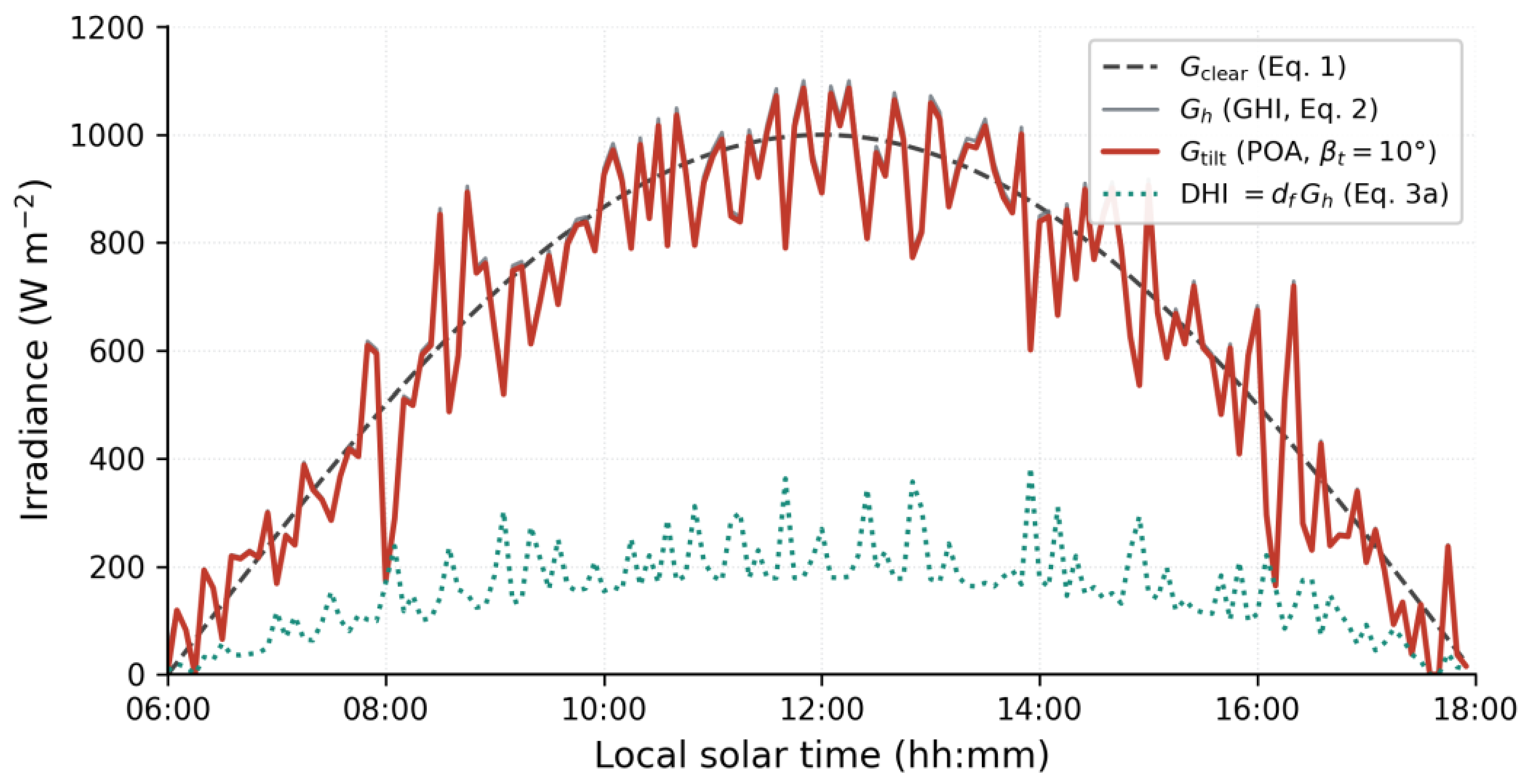
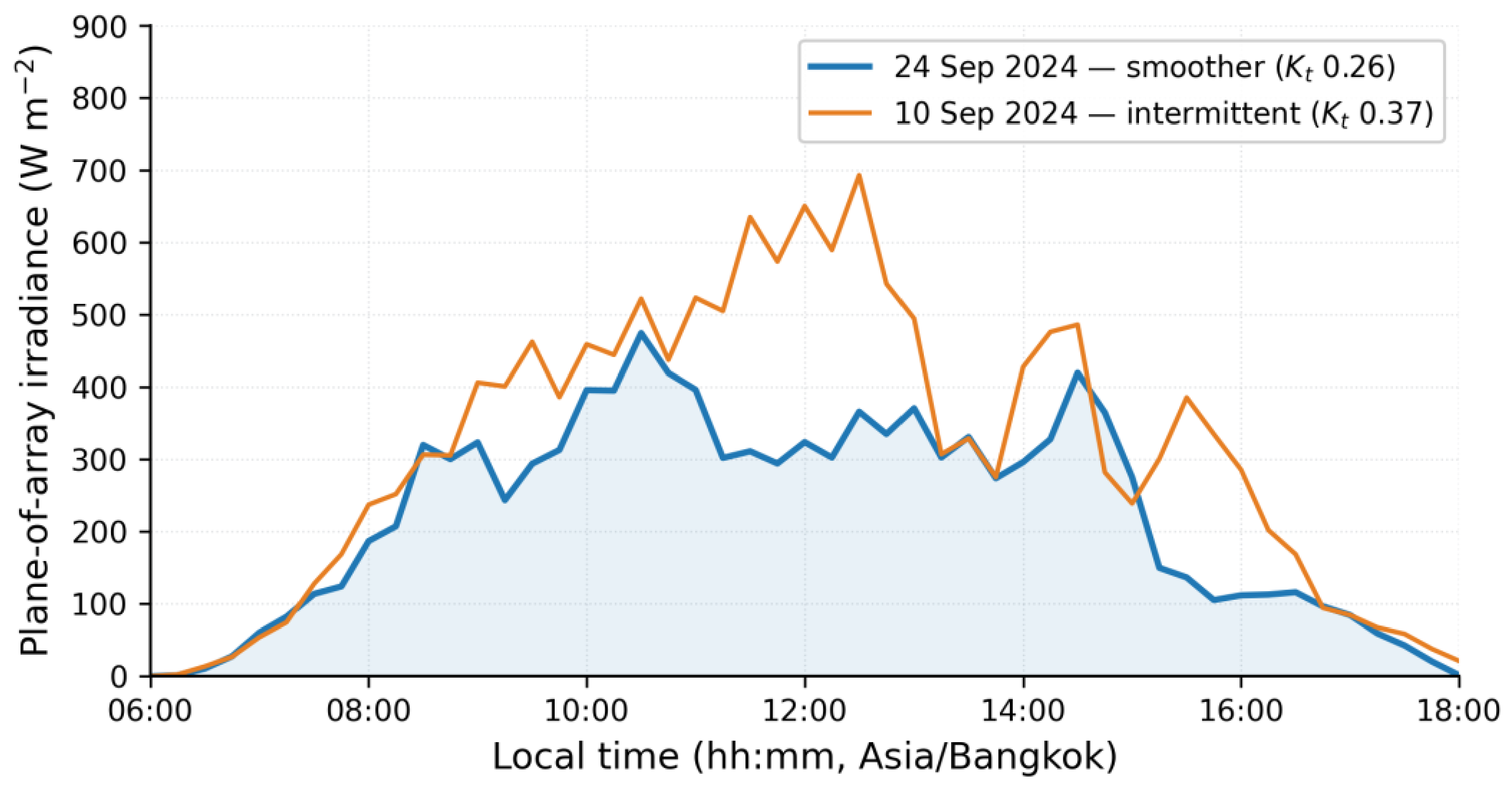
Figure 2 plots a single realisation of the stochastic forcing alongside the corresponding plane-of-array (POA) irradiance; its realism is corroborated in Section 3.6, where measured POA irradiance for two monsoon days of differing variability at the same site shares the diurnal envelope and cloud-driven intermittency (Figure 3).

The simulation date is n_d = 81 (vernal equinox, 22 March), representative of the annual-mean solar geometry for the site. The POA irradiance is obtained by isotropic-sky transposition [26], with the diffuse fraction d_f computed from the full three-branch Erbs (1982) correlation [27]:

$$d_f=\left\{\begin{array}{ll}1-0.09\hspace{0.17em}{k}_t,& k_t\le 0.22\\ 0.9511-0.1604\hspace{0.17em}{k}_t+4.388\hspace{0.17em}{k}_t^2-16.638\hspace{0.17em}{k}_t^3+12.336\hspace{0.17em}{k}_t^4,& 0.22<k_t\le 0.80\\ 0.165,& k_t>0.80\end{array}\right.$$

(3)

The Python implementation of Equation (3) is given in Listing S1 (Supplementary Materials). The corresponding routine in the original notebook used only the first and third branches, biassing the POA irradiance upward by 30–80% for partly cloudy conditions (0.22 < k_t < 0.80); the corrected form is used throughout this study.

The diffuse fraction d_f splits the GHI into its diffuse and beam horizontal components, which are transposed to the plane of array by the isotropic-sky (Liu–Jordan) model [26]. With the day number n_d, solar declination δ = 23.45° sin [360°(284 + n_d)/365], hour angle ω = 15°(t − 12) and zenith angle given by cos θ_z = sin φ sin δ + cos φ cos δ cos ω at the site latitude φ = 8.643° N, the instantaneous clearness index is k_t = G_h/(G_sc cos θ_z), with G_sc = 1367 W m⁻²; then

$$\mathrm{D}\mathrm{H}\mathrm{I}=d_f\hspace{0.17em}{G}_h, \mathrm{B}\mathrm{H}\mathrm{I}=G_h-\mathrm{D}\mathrm{H}\mathrm{I}$$

(3a)

$$G_{\mathrm{t}\mathrm{i}\mathrm{l}\mathrm{t}}=\mathrm{B}\mathrm{H}\mathrm{I}\hspace{0.17em}{R}_b+\mathrm{D}\mathrm{H}\mathrm{I}\hspace{0.17em}{\displaystyle \frac{1+\mathrm{c}\mathrm{o}\mathrm{s}{\beta }_t}{2}}+G_h\hspace{0.17em}\rho \hspace{0.17em}{\displaystyle \frac{1-\mathrm{c}\mathrm{o}\mathrm{s}{\beta }_t}{2}}, R_b={\displaystyle \frac{\mathrm{c}\mathrm{o}\mathrm{s}\theta }{\mathrm{c}\mathrm{o}\mathrm{s}{\theta }_z}}$$

(3b)

where β_t = 10° is the collector tilt, ρ = 0.20 the ground albedo and cos θ = cos θ_z cos β_t for the south-facing collector. Equation (3b) defines the plane-of-array irradiance G_tilt used throughout (Equations (5), (6), (13a) and (14)); at this small tilt and low latitude R_b ≈ 1, which is why the POA tracks the GHI closely in Figure 2 and Figure 3.

3.2. Eight-Layer PVT Model

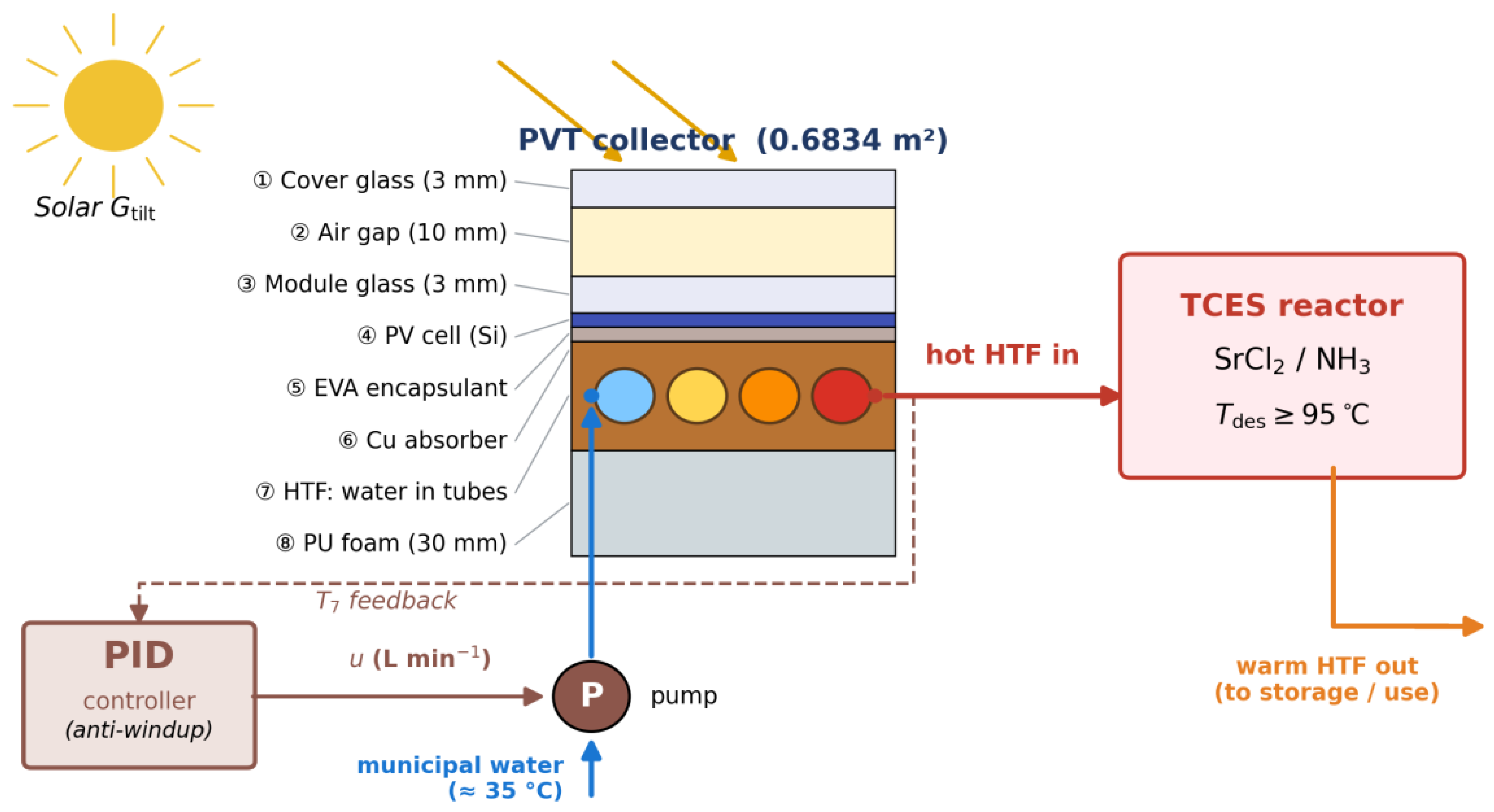
The collector is modelled as a one-dimensional lumped-capacitance system comprising eight thermal nodes, numbered ①–⑧ in Figure 1: (1) cover glass, (2) air gap, (3) module glass, (4) PV cell, (5) EVA adhesive, (6) copper absorber and tube, (7) HTF, and (8) PU foam back-insulation. The PV electrical efficiency is temperature-dependent:

$$\eta (T_4)={\eta }_{\mathrm{r}\mathrm{e}\mathrm{f}}\left[\hspace{0.17em}1-\beta \hspace{0.17em}(T_4-T_{\mathrm{r}\mathrm{e}\mathrm{f}})\hspace{0.17em}\right]$$

(4)

$$P_{\mathrm{e}\mathrm{l}\mathrm{e}\mathrm{c}}=\eta (T_4)\hspace{0.17em}{G}_{\mathrm{t}\mathrm{i}\mathrm{l}\mathrm{t}}\hspace{0.17em}{\tau }_{\mathrm{c}\mathrm{o}\mathrm{v}}\hspace{0.17em}{\tau }_{\mathrm{m}\mathrm{o}\mathrm{d}}\hspace{0.17em}A$$

(5)

The energy balance equation for the PV-cell node (illustrative of the formulation; the complete eight-equation system is written out in Appendix B and implemented in Listing S2 of the Supplementary Materials) is:

$$m_4{c}_4{\displaystyle \frac{d{T}_4}{dt}}={\alpha }_{\mathrm{p}\mathrm{v}}{\tau }_{\mathrm{c}\mathrm{o}\mathrm{v}}{\tau }_{\mathrm{m}\mathrm{o}\mathrm{d}}{G}_{\mathrm{t}\mathrm{i}\mathrm{l}\mathrm{t}}A-P_{\mathrm{e}\mathrm{l}\mathrm{e}\mathrm{c}}+h_{\mathrm{c}\mathrm{o}\mathrm{n}\mathrm{d}}A(T_3-T_4)-h_{\mathrm{c}\mathrm{o}\mathrm{n}\mathrm{d}}A(T_4-T_5)$$

(6)

Here h_cond = 200 W m⁻² K⁻¹ is the solid inter-layer conduction coefficient (

Table 2. System parameters (PVT collector and PID controller).

Parameter	Symbol	Value	Unit
Collector aperture area	A	0.6834	m2
Tube–fluid contact area	Atube	0.41	m2
Reference electrical efficiency (STC)	ηref	0.16	–
Temperature coefficient	β	0.0045	K−1
STC reference temperature	Tref	25	°C
Sky radiation coefficient	hrad	5.0	W m−2 K−1
Tube-to-fluid convection	hfluid	350	W m−2 K−1
PU foam back loss coefficient	hins	0.83	W m−2 K−1
Inter-layer (solid) conduction coefficient	hcond	200	W m−2 K−1
Air-gap conduction coefficient	hgap	5.5	W m−2 K−1
Cover-glass absorptance	αglass	0.04	–
Cover glass transmittance	τcov	0.91	–
Module glass transmittance	τmod	0.92	–
PV cell absorptance	αpv	0.90	–
HTF inlet temperature (municipal once-through feed)	Tin	35	°C
Exergy dead-state (reference) temperature	Ta(t)	instantaneous ambient	°C
PID setpoint (TCES threshold)	Tsp	95	°C
PID proportional gain	Kp	0.015	–
PID integral gain	Ki	2 × 10−4	–
PID derivative gain	Kd	0.20	–
Control timestep	Δt	10	s
Pump flow range	[umin, umax]	[0.05, 0.5]	L min−1

), applied over the aperture area A to each internal solid–solid link (nodes ③–④, ④–⑤, ⑤–⑥ and ⑥–⑧); the glazing stack (nodes ①–②–③) is coupled through the air-gap coefficient h_gap = 5.5 W m⁻² K⁻¹, and the cover glass absorbs a fraction α_glass = 0.04 of the incident irradiance. The complete eight-equation system is written out in Appendix B, and the nodal masses and heat capacities are listed in

Table 3. Nodal masses, specific heats and lumped heat capacities of the eight-node model (nodes ①–⑧ of Figure 1; transcribed from the released implementation).

Node	Component	m (kg)	c (J kg−1 K−1)	m·c (J K−1)
①	Cover glass	5.1	800	4080
②	Air gap	0.008	1005	8.0
③	Module glass	5.1	800	4080
④	PV cell	0.5	800	400
⑤	EVA adhesive	0.5	2000	1000
⑥	Copper absorber + tube	3.0	385	1155
⑦	HTF (water, 0.8 L)	0.8	4180	3344
⑧	PU foam back	0.82	1500	1230

.

The fluid-node energy balance (which is the algebraic linkage to the PID actuator) is:

$$m_7{c}_7{\displaystyle \frac{d{T}_7}{dt}}=h_{\mathrm{f}\mathrm{l}\mathrm{u}\mathrm{i}\mathrm{d}}{A}_{\mathrm{t}\mathrm{u}\mathrm{b}\mathrm{e}}\left(T_6-T_7\right)-\dot{m}\hspace{0.17em}{c}_{p,w}(T_7-T_{\mathrm{i}\mathrm{n}})$$

(7)

The useful thermal heat removal rate that defines the input to the TCES reactor is:

$${\dot{Q}}_{\mathrm{t}\mathrm{h}}(t)=\dot{m}(t)\hspace{0.17em}{c}_{p,w}\left[T_7(t)-T_{\mathrm{i}\mathrm{n}}\right]$$

(8)

The front-side convection coefficient depends on wind speed via the McAdams correlation, h_conv(v) = 5.7 + 3.8 v (in W m⁻² K⁻¹), so that the simulation responds correctly to the diurnal wind profile:

$$h_{\mathrm{c}\mathrm{o}\mathrm{n}\mathrm{v}}(v)=5.7+3.8\hspace{0.17em}v$$

(9)

The eight coupled ODEs are integrated over each control interval Δt = 10 s using scipy.integrate.odeint with relative and absolute tolerances of 1 × 10⁻⁶ and 1 × 10⁻⁸ respectively and a maximum internal step size of 1 s. Initial conditions are set to the ambient temperature at simulation start (06:00). Physical and control parameters are listed in Table 2.

The modelled aperture A = 0.6834 m² is the reference collector used consistently throughout this modelling programme; the experimental prototype of Section 3.6 is a larger unit (full Jinko JKM355PP-72 module, ≈1.94 m² aperture) used to validate the intensive collector heat transfer physics at a different scale. Because every reported efficiency is a per-unit-area ratio, a 2.8× change in aperture (0.6834 → 1.94 m², with nodal masses and flow limits scaled) changes the first- and second-law efficiencies by less than 0.5%, while absolute yields scale linearly.

3.3. PID Controller

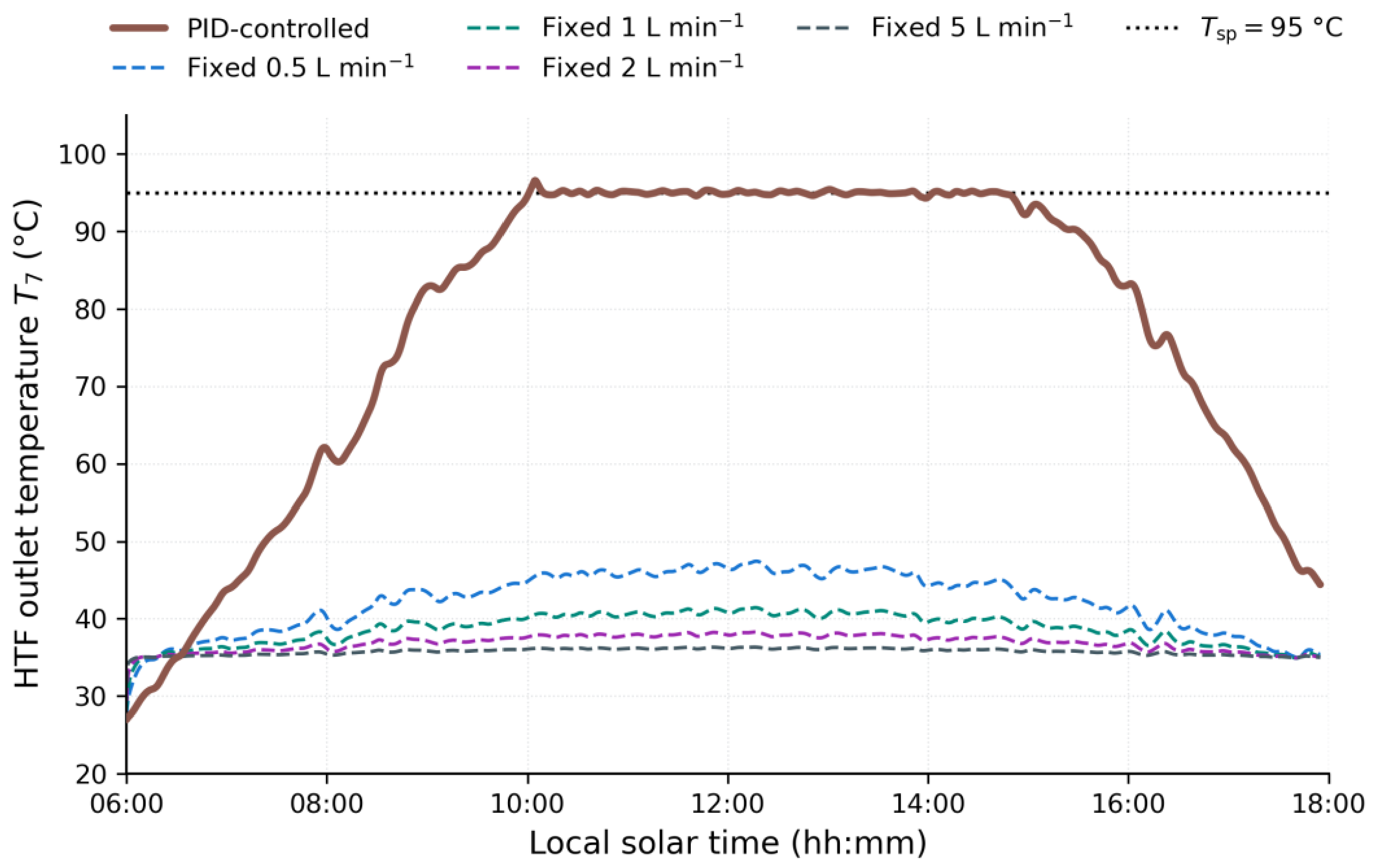
A discrete-time PID controller regulates the pump flow rate u(k) with the objective of holding the HTF outlet temperature T₇ at the setpoint T_sp = 95 °C, corresponding to the SrCl₂/NH₃ desorption threshold. The error and the control law are:

$$e(k)=T_7(k)-T_{\mathrm{s}\mathrm{p}}$$

(10)

$$u(k)=K_p\hspace{0.17em}e(k)+K_i{\displaystyle {\sum }_{j=0}^k}e(j)\hspace{0.17em}\mathsf{\Delta }t+K_d\hspace{0.17em}{\displaystyle \frac{e(k)-e(k-1)}{\mathsf{\Delta }t}}$$

(11)

In Equation (11), k is the current discrete control step, j is the summation (integration) index running over control steps 0, …, k, e(j) is the outlet temperature error of Equation (10) at step j, and Δt = 10 s is the control interval, so the middle term is the accumulated integral error. The regulated (controlled) variable is the outlet temperature T₇—a measurable proxy for the reactor desorption threshold constraint—not exergy directly; the energy and exergy quantities of Section 3.4 are performance evaluation metrics computed from the resulting trajectories, not control objectives.

The controller output is bounded to [u_min, u_max] = [0.05, 0.5] L min⁻¹. Conditional-integration anti-windup is implemented: when saturated at u_max, the integral updates only if e < 0; when saturated at u_min, only if e > 0. This prevents exergy-destroying overshoot when the controller emerges from a saturated state—a condition that recurs repeatedly under cloud transients. The PID implementation is given in Listing S3 (Supplementary Materials).

The control variable u is treated as an idealised bounded flow command; the physical actuator is a small variable-speed circulation pump, and its finite turndown and minimum stable flow are the practical constraints on realising the low-flow regime the controller commands. The 0.05–0.10 L min⁻¹ active band identified below is not a modelling abstraction: the co-located PVT prototype of Section 3.6 is driven by a 12 V DC circulation pump that sustains stable outlet temperature regulation in precisely this band under monsoon operation, demonstrating that an embedded-systems-cost pump can deliver the ultra-low flow on which the desorption threshold temperature rise depends. The ≈60 K per-pass rise required to reach the TCES setpoint is achievable only at flows roughly an order of magnitude below the typical PVT design point; that this is the regime in which small pumps approach their low-flow stability limit is precisely why deployability, not control sophistication, is the decisive lever for this system class (Section 5.1).

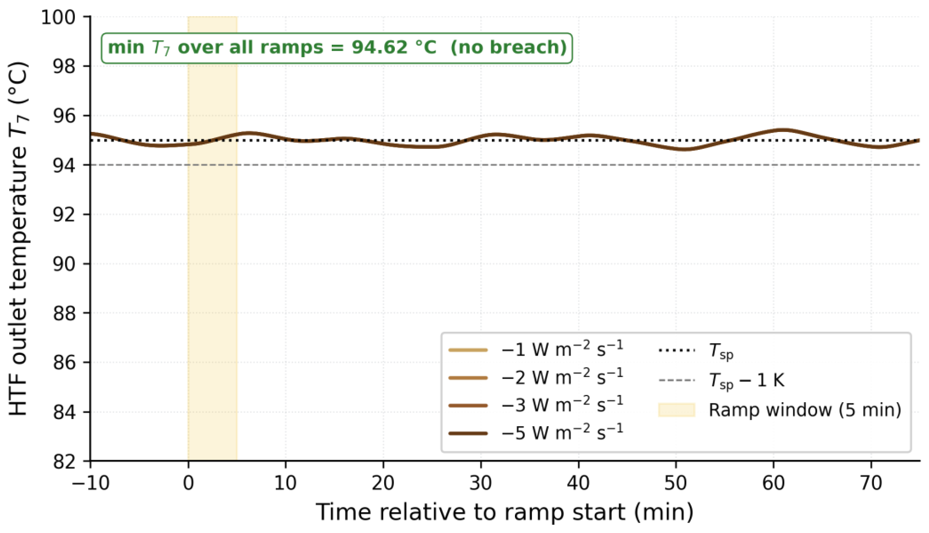
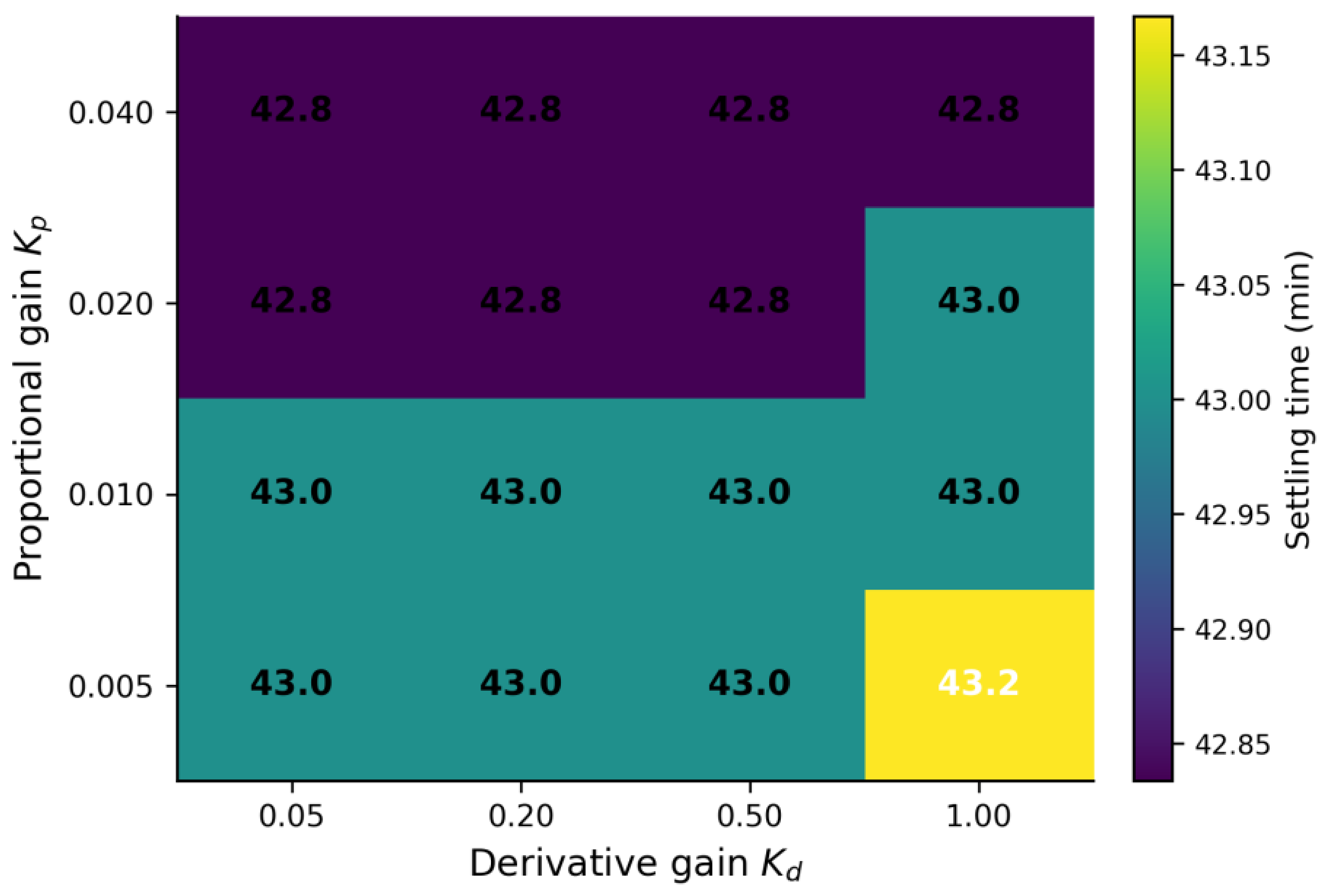
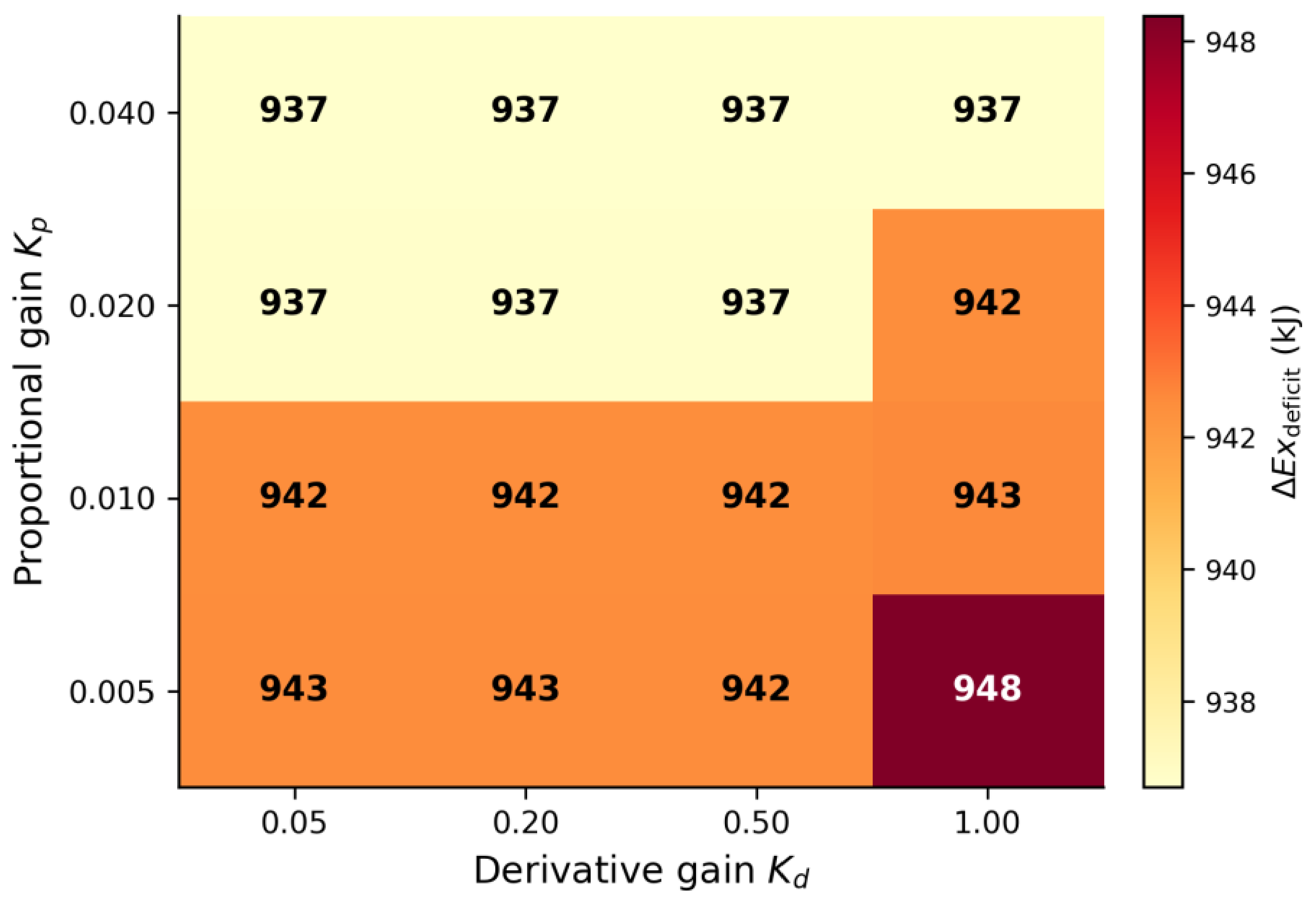
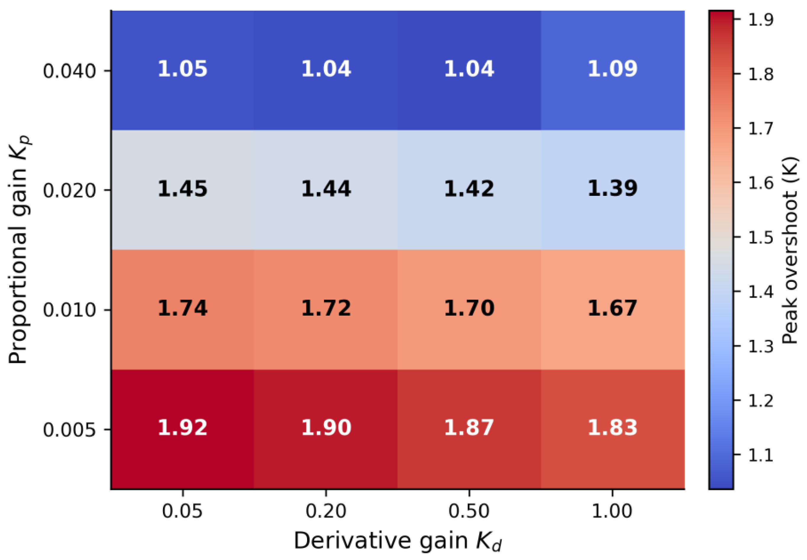
The gain set was selected by manual sensitivity tuning informed by the plant’s identified input-to-outlet response time: at the noon operating point, a step in irradiance or flow relaxes with an effective 63% response time τ_eff ≈ 13–15 min, dominated by the thermally coupled glazing stack (the bare absorber-plus-fluid estimate (m₆c₆ + m₇c₇)/(h_fluid A_tube) ≈ 31 s is far shorter; Table 3, Appendix B). Gains an order of magnitude faster or slower than the adopted set were rejected as noise-amplifying or sluggish. We do not claim a formal optimal-tuning procedure: the 4 × 4 sweep of Section 4.5 confirms a posteriori that the principal transient metrics vary by at most a few percent across the swept range, so the central conclusions do not depend on the precise gain values.

3.4. Energy and Exergy Performance Metrics

Throughout the exergy analysis the dead state (reference environment) is the instantaneous ambient temperature T_a(t)—the same time-varying ambient that forces the collector energy balance (Table 2); it is distinct from the STC reference temperature T_ref = 25 °C of the PV model (Equation (4)) and from the HTF inlet temperature T_in = 35 °C. All exergy efficiencies reported here are gross values: they are referenced to the collector control volume (aperture to HTF outlet) and exclude pump electrical consumption. At the throttled operating band (0.05–0.10 L min⁻¹) the pumping penalty is small—the ideal hydraulic exergy is ≈0.03 W (≈0.007% of the daily exergy yield), and even a realistic 12 V DC circulation pump drawing ≈5 W while energised consumes ≈7 Wh day⁻¹ at the 11.6% mean duty cycle, i.e., ≈1% of the total daily exergy yield—so the net exergy efficiency lies within about one relative percent of the gross value quoted throughout.

The thermal exergy delivered to the TCES reactor is computed from the rigorous Bejan/Kotas integrated form [28], which accounts for the cooling of the HTF as it transfers heat from T₇ to T_in:

$${\dot{Ex}}_{\mathrm{t}\mathrm{h}}(t)=\dot{m}(t)\hspace{0.17em}{c}_{p,w}\left\{\hspace{0.17em}[\hspace{0.17em}{T}_7(t)-T_{\mathrm{i}\mathrm{n}}\hspace{0.17em}]-T_a(t)\hspace{0.17em}\mathrm{l}\mathrm{n}{\displaystyle \frac{T_7(t)}{T_{\mathrm{i}\mathrm{n}}}}\hspace{0.17em}\right\}$$

(12)

The implementation is given in Listing S4 (Supplementary Materials). The constant-temperature approximation used in earlier PVT exergy work overestimates the thermal exergy by about 22% at the present operating point (Section 4.1, Figure S6).

The solar exergy uses the temperature-dependent Petela coefficient [29]:

$$\psi (T_a)=1-{\displaystyle \frac{4}{3}}\left({\displaystyle \frac{T_a}{T_{\odot }}}\right)+{\displaystyle \frac{1}{3}}{\left({\displaystyle \frac{T_a}{T_{\odot }}}\right)}^4$$

(13)

The solar and electrical exergy rates follow directly—electricity is pure exergy, and the solar exergy is the Petela-weighted plane-of-array irradiance:

$${\dot{Ex}}_{\mathrm{s}\mathrm{o}\mathrm{l}\mathrm{a}\mathrm{r}}(t)=\psi \left(T_a(t)\right)\hspace{0.17em}{G}_{\mathrm{t}\mathrm{i}\mathrm{l}\mathrm{t}}(t)\hspace{0.17em}A$$

(13a)

$${\dot{Ex}}_{\mathrm{e}\mathrm{l}\mathrm{e}\mathrm{c}}(t)=P_{\mathrm{e}\mathrm{l}\mathrm{e}\mathrm{c}}(t)$$

(13b)

Writing a second-law (exergy) balance over the collector control volume—bounded by the aperture (solar exergy inflow) and the HTF outlet (thermal exergy outflow to the reactor), with dead state T_a(t)—gives Ėx_solar = Ėx_elec + Ėx_th + Ėx_loss + T_a·$\stackrel{.}{\mathrm{S}}$_gen, where Ėx_loss collects the exergy carried away by the convective, radiative and back-insulation losses and T_a·$\stackrel{.}{\mathrm{S}}$_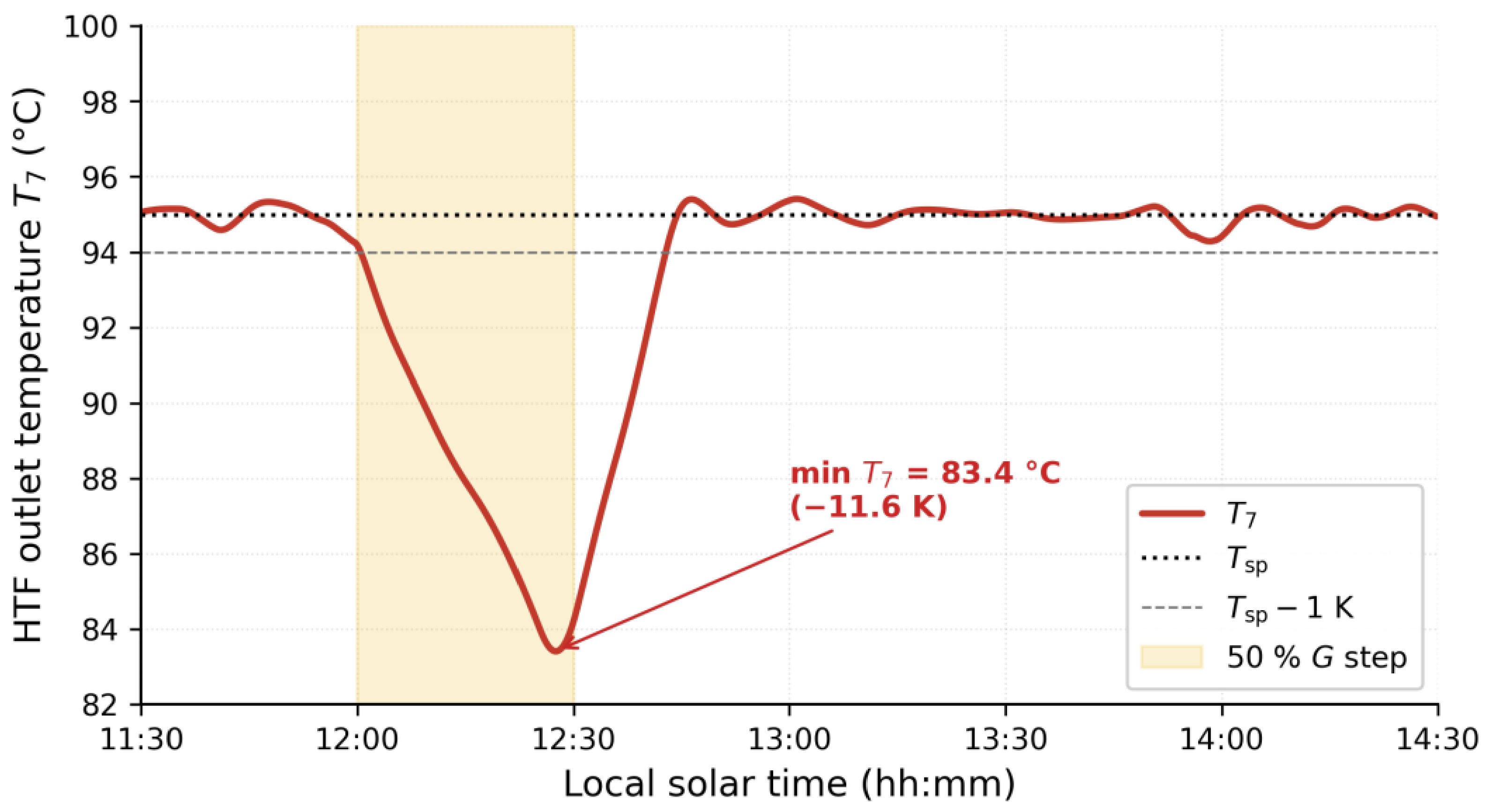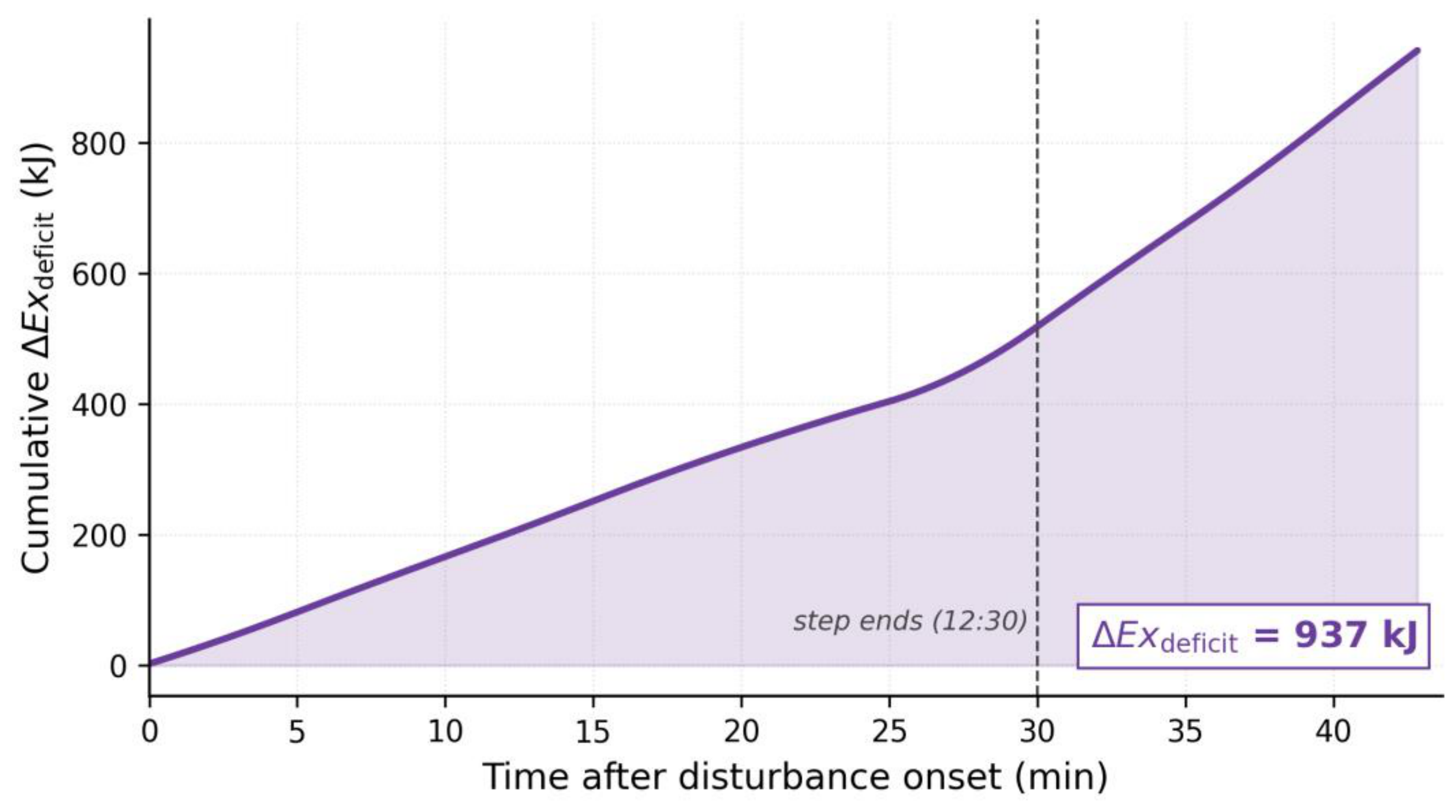gen is the internal irreversibility. The principal novelty metric of this paper is the exergy that fails to reach the reactor, relative to the undisturbed baseline, during a PID recovery transient—the accumulated exergy delivery deficit:

$$\mathsf{\Delta }E{x}_{\mathrm{d}\mathrm{e}\mathrm{f}\mathrm{i}\mathrm{c}\mathrm{i}\mathrm{t}}={\int }_{t_{\mathrm{d}\mathrm{i}\mathrm{s}\mathrm{t}}}^{t_{\mathrm{s}\mathrm{e}\mathrm{t}\mathrm{t}\mathrm{l}\mathrm{e}}}\left[\hspace{0.17em}\psi \left(T_a(t)\right)\hspace{0.17em}{G}_{\mathrm{t}\mathrm{i}\mathrm{l}\mathrm{t}}(t)\hspace{0.17em}A-P_{\mathrm{e}\mathrm{l}\mathrm{e}\mathrm{c}}(t)-\dot{m}(t)\hspace{0.17em}{c}_{p,w}\left\{\left(T_7(t)-T_{\mathrm{i}\mathrm{n}}\right)-T_a(t)\hspace{0.17em}\mathrm{l}\mathrm{n}{\displaystyle \frac{T_7(t)}{T_{\mathrm{i}\mathrm{n}}}}\right\}\hspace{0.17em}\right]\hspace{0.17em}dt$$

(14)

with t_dist the disturbance onset, t_settle the time at which T₇ returns to within 1 K of T_sp, and the three integrand terms given by Equations (13a), (13b) and (12) at the common dead state T_a(t). By the control-volume balance above, the integrand equals Ėx_loss + T_a·$\stackrel{.}{\mathrm{S}}$_gen: the metric measures undelivered exergy relative to the undisturbed baseline, not internal irreversibility alone—during an irradiance reduction it is dominated by the un-captured solar term, the true irreversibility being only the recovery-transient subset. This is precisely why, as shown in Section 4.5, ΔEx_deficit is a controller-independent benchmark for the configuration: the controller can act only on the small recovery-transient term.

3.5. Case Studies

Table 4. Summary of the five case-study scenarios.

Case	Disturbance/Setup	Reported Metrics
1	Full-day stochastic forcing, Monte-Carlo (N = 30 seeds)	Daily energy + exergy yields, peak temperatures, time at Tsp
2	50% step reduction in Gtilt at solar noon, 30 min hold	Settling time, undershoot, overshoot, ΔExdeficit (Equation (14))
3	Sustained linear ramps at −1, −2, −3, −5 W m−2 s−1 for 5 min	Minimum HTF outlet temperature, threshold-breach assessment
4	PID vs. fixed flow at u ∈ {0.5, 1.0, 2.0, 5.0} L min−1	Peak Tout, peak Tpv, time at Tsp
5	4 × 4 grid in (Kp, Kd), 0.33–2.7× and 0.25–5× of nominal	Heat-maps of settling time, ΔExdeficit, overshoot

summarises the five case-study scenarios examined in this section; each case isolates one aspect of the controller’s dynamic response and its exergy consequences.

3.6. Experimental Validation and Real-Weather Forcing

The thermal model of Section 3.2 and the irradiance forcing of Section 3.1 are grounded here against measured data from the study site. Two independent sources are used. The first is a three-year record (March 2023 to June 2026) from the Walailak University rooftop monitoring system of a 2.54 MWp grid-connected photovoltaic plant, logging plane-of-array irradiance from two independent pyranometers (and their geometric mean), ambient temperature, module temperature and wind speed at 15 min resolution. The second is a purpose-built single-panel PVT collector—a Jinko JKM355PP-72 module fitted with a copper-tube absorber, foam-insulated back and glazed front, regulated by a PID-controlled 12 V DC circulation pump acting on the outlet water temperature and operating in the same 0.05–0.10 L min⁻¹ band as the simulated controller command (Section 3.3)—constructed and instrumented at the same site. The prototype module (≈1.94 m² aperture) is larger than the 0.6834 m² modelled reference collector; because the validation compares temperatures and per-area heat transfer coefficients, it tests the collector heat transfer physics at a different scale rather than the modelled once-through temperature rise. Because the prototype construction (cover → air gap → module glass → cell → absorber/tube → fluid → insulated back) mirrors the eight-node stack of Section 3.2, and because its pump controller is a physical instance of the flow rate feedback law studied in this paper, it provides a partial but well-posed hardware test of both the collector physics and the control concept.

Measured forcing is reconstructed by transposing the WU global horizontal irradiance to the plane of array with the same optics used in Section 3.1 (Erbs diffuse split, isotropic sky). Figure 3 overlays the two September 2024 prototype-campaign days, which differ in daily clearness and sub-daily variability (both cloud-affected—neither is a clear-sky day). The measured envelope and its cloud-driven excursions are consistent with the synthetic forcing of Figure 2, confirming that the σ = 120 W m⁻² stochastic model is representative of the site; the three-year record additionally supplies many genuinely clear and intermittent days that are retained as drop-in forcing for the planned multi-day analysis. Note that the smoother campaign day (24 September, K_t = 0.26) has a lower daily clearness index than the more intermittent day (10 September, K_t = 0.37): within a cloudy monsoon fortnight, daily transmittance and sub-daily variability are only weakly correlated, so the day with fewer fast fluctuations is not necessarily the brighter one.

Table 5. All irradiance days used in this study.

Label	Date	Source	Kt	VI	Role
Synthetic stochastic day	nd = 81 (22 March)	Equations (1) and (2), σG = 120 W m−2	≈0.7	–	Cases 1–5 forcing (Section 4)
Synthetic clear archetype	–	shared-plant generator	0.74	1.03	Appendix A.2
Synthetic intermittent archetype	–	shared-plant generator	0.72	1.27	Appendix A.2
Measured—smoother	24 September 2024	WU pyranometers	0.26	low	Section 3.6 validation
Measured—intermittent	10 September 2024	WU pyranometers	0.37	high	Section 3.6 validation
Measured—clear-sky	23 February 2026	WU pyranometers	0.52	1.00	Section 6 output (abstract headline)
Measured—overcast	7 May 2024	WU pyranometers	0.13	1.00	Section 6 output

collates every measured and synthetic day used in this study.

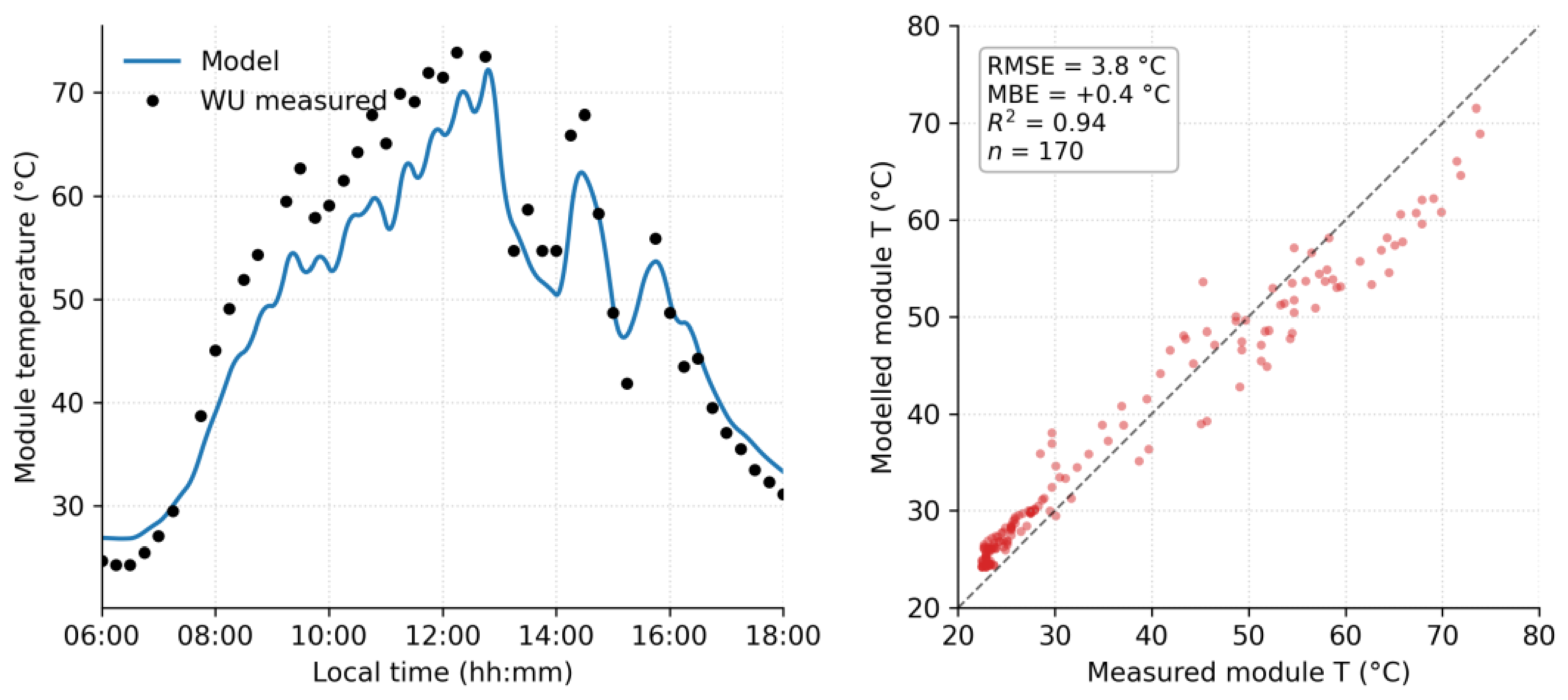
The front-side thermal core of the model—the optics and the convective/radiative balance of nodes 1–4, which set the cell operating temperature and hence both the η(T) penalty and the exergy delivery deficit benchmark—is validated against the measured temperature of a bare rooftop PV module driven by the WU plane-of-array irradiance, ambient temperature and wind. Integrating the lumped energy balance C·dT_m/dt = (ατ − η(T_m))·G_POA − U(v)·(T_m − T_a), with a single site-calibrated loss coefficient (U ≈ 12 W m⁻² K⁻¹, consistent with the restricted ventilation of the close-mounted array, NOCT-equivalent ≈ 57 °C), reproduces the measured module temperature with an RMSE of 3.8 °C, a mean bias of +0.4 °C and R² = 0.94 over n = 170 fifteen-minute samples (Figure 4). The model captures both the diurnal envelope and the cloud-driven dips and relaxes to 1–2 °C below ambient at night, the correct radiative behaviour. This supports the optical and convective/radiative physics that underpins the exergy delivery deficit benchmark.

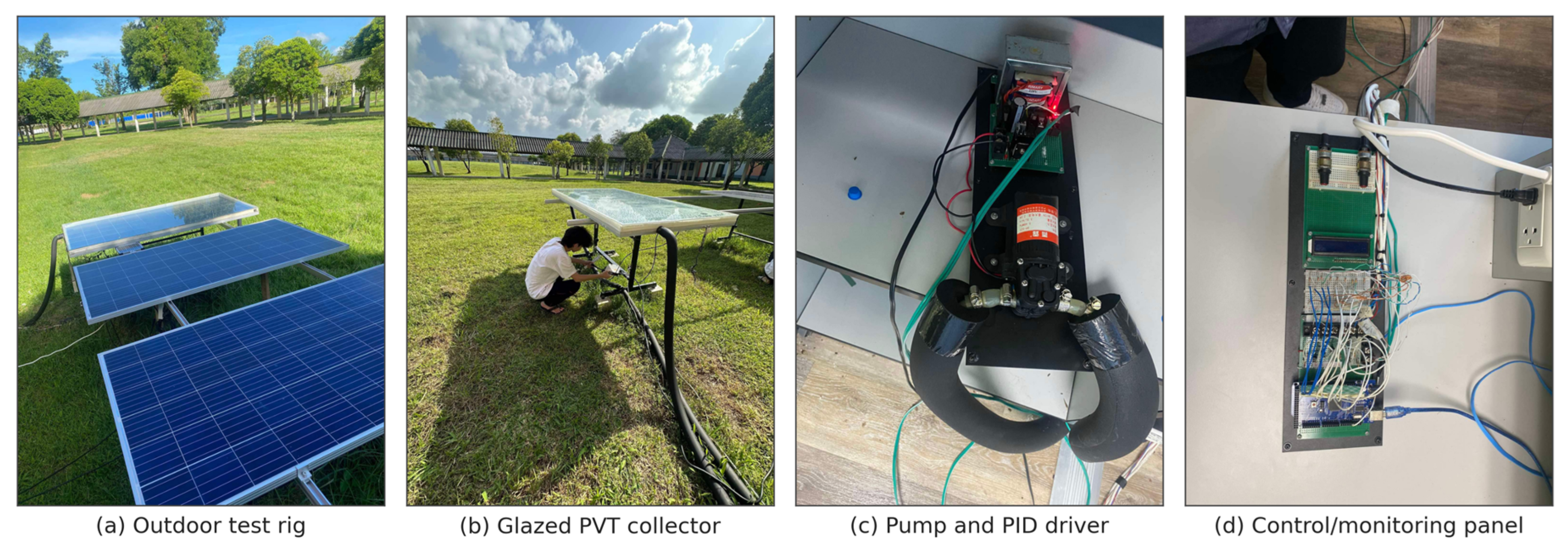
Figure 5 shows the prototype rig: the glazed copper-tube PVT collector, the variable-speed circulation pump and its PID driver, and the control and data-acquisition panel. The controller modulates the 12 V pump to regulate the outlet water temperature—the same flow rate feedback principle analysed throughout this paper—and the rig was operated outdoors under September monsoon skies. On-site irradiance was not logged during these (rainy) campaigns, which is precisely why the co-located WU pyranometer record supplies the forcing for the prototype analysis.

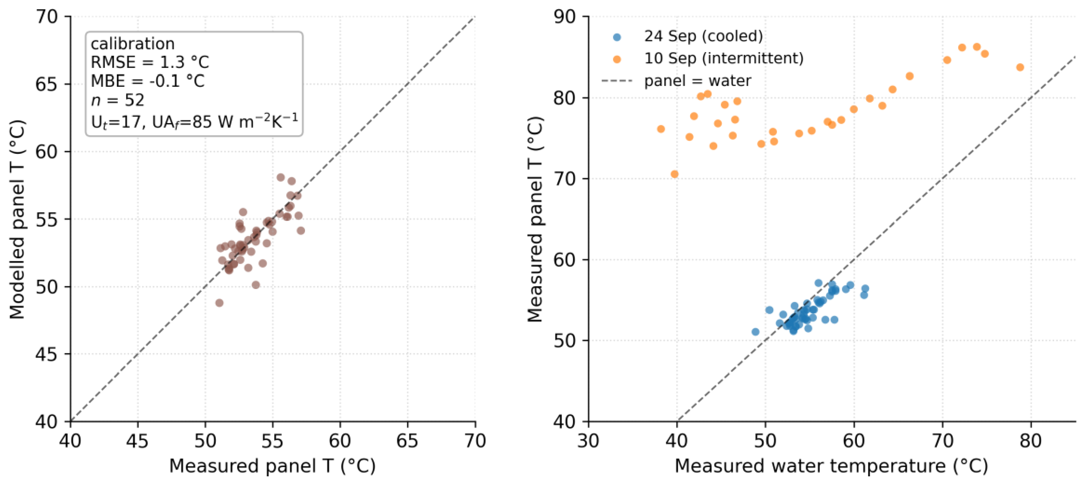
Because the prototype water inlet temperature was not logged, the panel temperature is predicted from the WU forcing using the measured outlet water temperature as the fluid boundary condition, which isolates the absorber-to-water heat transfer physics. On the well-cooled campaign day (24 September 2024, low-variability), the model reproduces the measured panel temperature with an RMSE of 1.3 °C (n = 52); the fitted absorber-to-water conductance, UA_f ≈ 85 W m⁻² K⁻¹, is high and consistent with well-bonded copper tubing (Figure 6, left). An adversarial baseline that simply equates panel and water temperature achieves only RMSE 2.1 °C, so the energy balance model improves the prediction by about 39% in RMSE—real structure rather than overfitting. On the intermittent day (10 September), with the pump cycling under fast cloud transients, the measured panel temperature sits well above the water temperature, and the fitted conductance collapses to ≈9 W m⁻² K⁻¹ (Figure 6, right): the model thus correctly reproduces flow-limited panel–water decoupling, the very mechanism that the flow rate controller of this paper exists to manage.

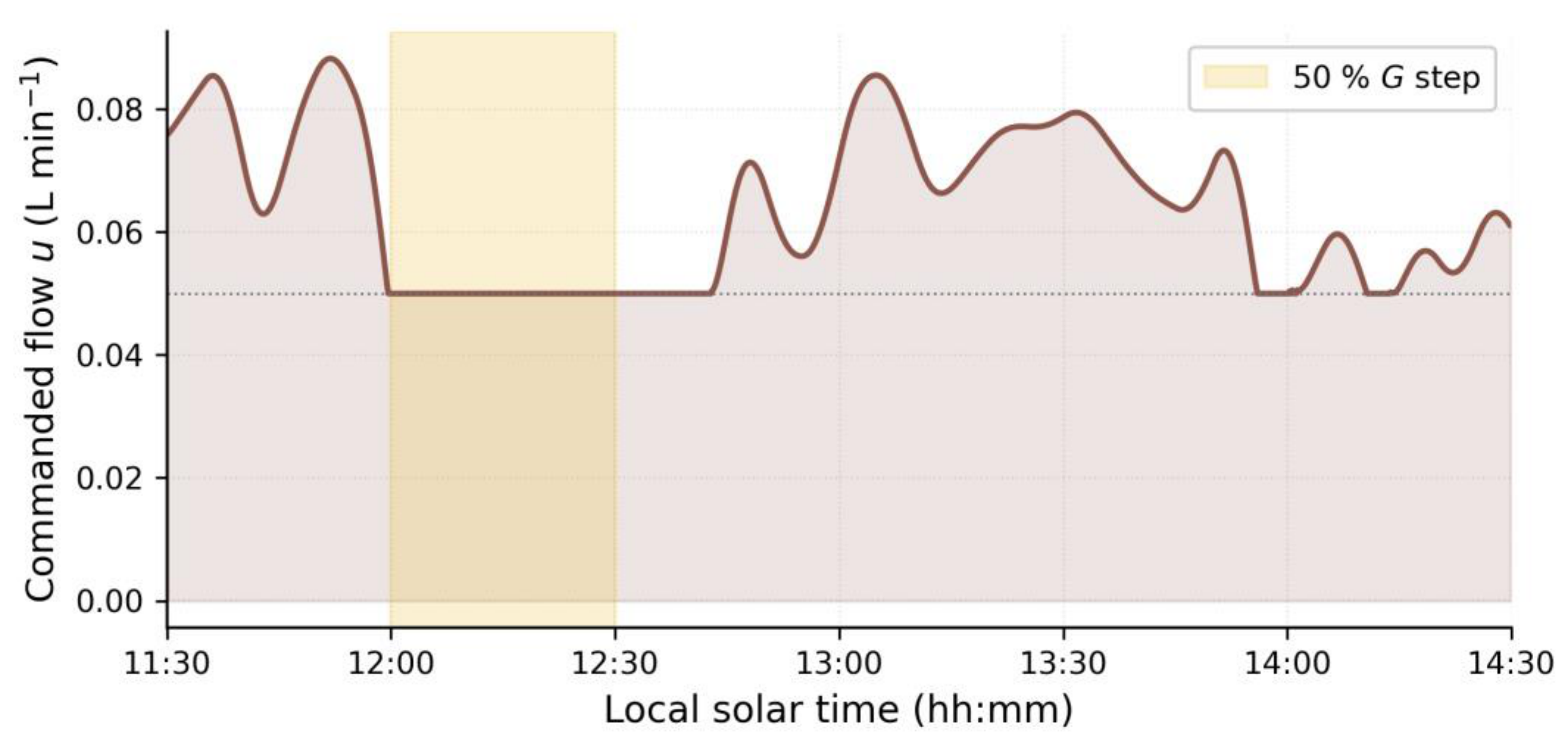
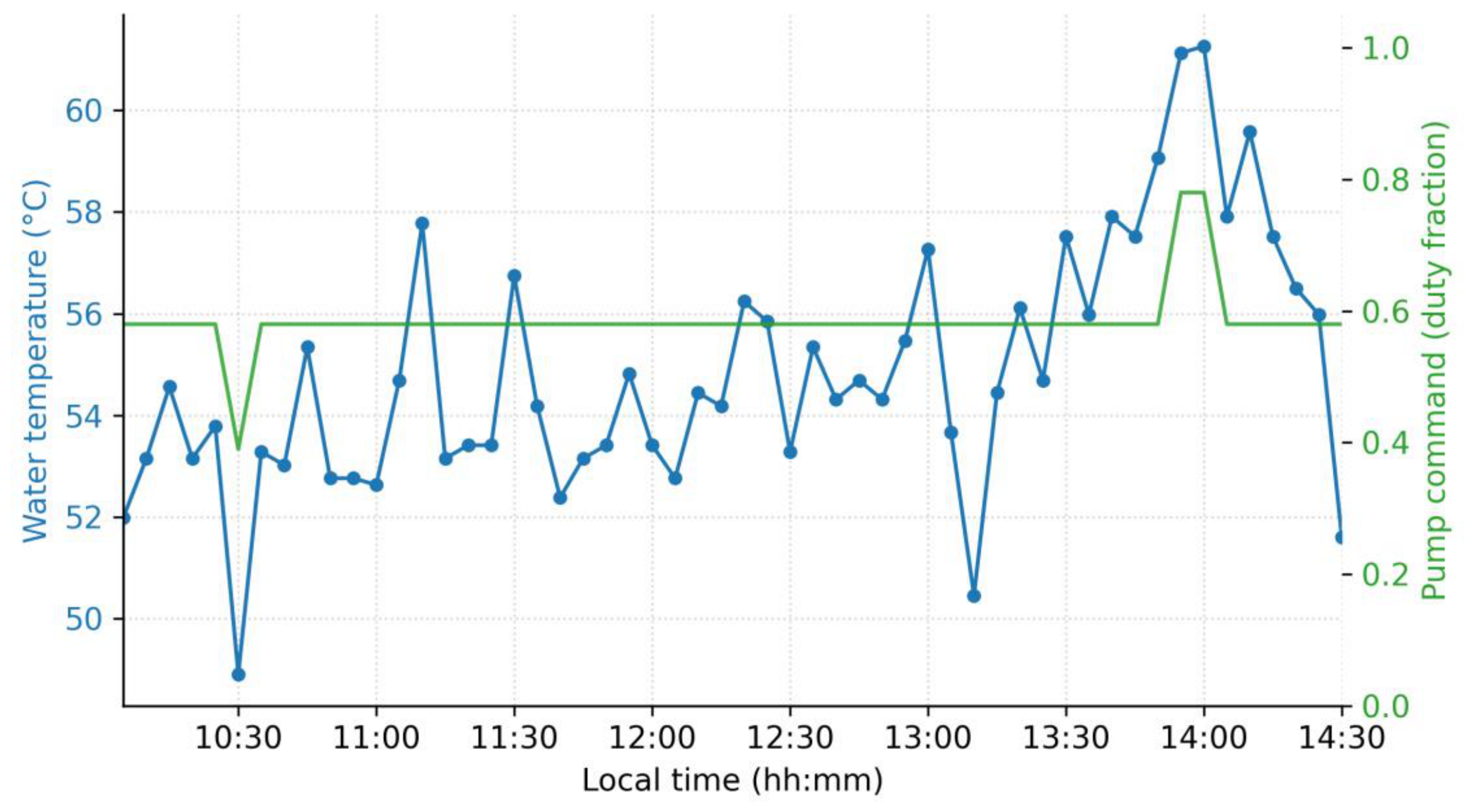
Under the same monsoon conditions, the prototype delivered usable hot water—a peak outlet up to 79 °C—daily maxima of 46–79 °C across the four campaign days (61–79 °C on the three non-stagnant days) and daily means of 39–56 °C—while the PID modulated the pump flow (Figure 7). This is a real-world demonstration of the PVT-to-TCES charging service that the simulated system is designed to provide: the controller trades a measure of electrical efficiency for a thermal stream hot enough to approach the desorption threshold, exactly as in the simulation.

The validation establishes the model’s thermal behaviour, not its electrical model: the prototype panel was not held at its maximum-power point, so the measured apparent efficiency (0.10–0.12, rising anomalously with temperature) could not validate the temperature-dependent η(T) relation, which is supported by the manufacturer datasheet and enters the thermal balance weakly (η·G_tilt ≪ ατ·G_tilt). The module validation addresses the front optical/convective core common to PV and PVT, and the cooled-collector validation demonstrates absorber/panel heat transfer rather than the full once-through rise; two of the four prototype days are flow-limited, and one module loss coefficient is site-calibrated. Within this scope the agreement is strong, and the central physics underpinning the 937 kJ deficit benchmark is experimentally supported.

4. Results

4.1. Case 1—Baseline Tracking Under Stochastic Irradiance

Figure S1 shows the closed-loop temperature response under a single realisation (seed = 1) of the stochastic irradiance forcing. After the morning warm-up of approximately 3.5 h, the controller reaches the 95 °C setpoint and holds the HTF outlet within +1.4 K for the remainder of the high-irradiance window. The PV cell temperature reaches 103.6 °C around solar noon—the deliberate trade-off of operating the panel hot to deliver heat at the SrCl₂/NH₃ desorption threshold.

Figure S2 shows the corresponding commanded pump flow rate. The controller operates in a narrow active band around 0.05–0.10 L min⁻¹, with the u_min = 0.05 L min⁻¹ bound active only during warm-up and at end-of-day. The very low actuator duty cycle is a direct consequence of the high temperature-rise constraint required by the TCES setpoint.

Figure S3 overlays the POA irradiance and the PV electrical power, which peaks at about 60 W around solar noon; the 5–10 W oscillation on P_elec originates from the PID flow modulation (reduced flow raises cell temperature and depresses electrical output, and vice versa).

Figure S4 reports the first-law efficiency timeline. The hybrid (electrical + thermal) efficiency settles around 52% during the productive window; the electrical share is suppressed to ≈9.3% by the high PV cell temperature, while the thermal share reaches ≈43%. Figure S5 presents the corresponding daily energy distribution for the seed-1 realisation: of its 5.08 kWh of solar input, 0.47 kWh (9.3%) is converted to electricity, 2.19 kWh (43.0%) is recovered as useful thermal energy, and 2.42 kWh (47.6%) is lost (the N = 30 ensemble means are 5.14, 0.479 and 2.209 kWh;

Table 6. Case 1 Monte-Carlo headline metrics (N = 30).

Metric	Mean ± σ	Unit
Total solar energy input	5.14 ± 0.07	kWh
Electrical energy yield	0.479 ± 0.007	kWh
Thermal energy yield	2.209 ± 0.041	kWh
Exergy yield (rigorous, Equation (12))	0.678 ± 0.010	kWh
Daily mean exergy efficiency (gross, pump work excluded)	14.26 ± 0.03	%
Peak HTF outlet temperature	96.4 ± 0.3	°C
Peak PV cell temperature	103.6 ± 0.13	°C
Mean pump duty cycle	11.63 ± 0.15	%
Time at Tsp (within ±2 K)	5.32 ± 0.25	h
Total water throughput	41.6 ± 0.5	L

).

Figure S6 directly compares the two thermal-exergy formulations. The constant-temperature approximation $\stackrel{.}{\mathrm{Q}}$·(1 − T_a/T_out) returns a daily exergy yield of 0.821 kWh, whereas the rigorous Bejan/Kotas integrated form (Equation (12)) returns 0.671 kWh—a 22% overestimate by the simple formulation. The corresponding daily mean exergy efficiency drops from 17.5% to 14.3%. This is not a small correction and should be applied as default in future PVT studies where the per-pass temperature rise is comparable to (T_in − T_a).

Figure S7 shows the time-resolved exergy decomposition under the corrected formulation. Electrical and thermal exergies are approximately equal in magnitude through the high-irradiance window, with the overall exergy efficiency η_ex (right axis) stable in the 14–18% band over the productive window.

Across a Monte-Carlo ensemble of N = 30 independent random seeds, the headline metrics are tightly clustered: daily exergy yield 0.678 ± 0.010 kWh (spanning 0.657–0.696 kWh across the 30 seeds); daily mean exergy efficiency 14.26 ± 0.03%; time at setpoint 5.3 ± 0.3 h; total water throughput 41.6 ± 0.5 L (Table 6). The ensemble standard deviations are below 1.5% of the means; consistent with the modest sample, we report this spread as a robustness check rather than as a tight statistical confidence interval. The single-realisation (seed = 1) yield is 0.671 kWh under the rigorous formulation—the value against which the constant-temperature overestimate is computed (0.821/0.671 ≈ 1.22, Section 4.1)—while the 0.678 kWh ensemble mean is the headline figure quoted throughout.

4.2. Case 2—Step Disturbance and PID Recovery

Figure 8 shows the PID response to a 50% step reduction in G_tilt imposed at solar noon and held for 30 min. As the step is applied, T₇ drops by 11.6 K below the setpoint, reaching a minimum of 83.4 °C. On disturbance removal, T₇ recovers within 12.8 min to within 1 K of the setpoint, with a modest overshoot of 1.6 K—well within the +2 K tolerance band imposed by the TCES reaction-protection constraint.

Figure 9 shows the corresponding pump flow response. The controller saturates at u_min during the step (when no actuation can recover the missing solar input) and then ramps the flow up smoothly on recovery.

Figure 10 reports the principal novelty metric: the cumulative exergy-delivery deficit during the disturbance and recovery transient (Equation (14)). Over the 42.8 min interval from disturbance onset to settling—the 30 min hold plus the 12.8 min recovery, the latter almost exactly one plant response time τ_eff (Section 3.3)—the integrated ΔEx_deficit reaches 937 kJ. The dotted vertical line marks the end of the irradiance step (t = 30 min): the linearly growing cumulative curve before this point indicates that the deficit is dominated by the irrecoverable solar exergy lost during the irradiance reduction itself—when no PVT control action can recover the missing input. This finding has direct implications for which control architectures will and will not improve the result (Section 5.3).

4.3. Case 3—PID Robustness to Sustained Irradiance Ramps

Figure 11 reports the PID response to sustained linear irradiance ramps imposed at solar noon over a 5 min window, with rates from −1 to −5 W m⁻² s⁻¹. Despite the very wide range tested—the worst case drops the deterministic irradiance to zero within the 5 min window—the controller maintains the HTF outlet temperature within −0.4 K of the setpoint in every case, with no breach of the T_sp − 1 K reaction protection band. The minimum T₇ observed across all four ramps is 94.62 °C, dominated by the cumulative stochastic background noise rather than the deterministic ramp.

The robustness has a two-part physical explanation: (i) the collector thermal mass (≈3 kg of copper absorber, node ⑥, m₆c₆ ≈ 1.16 kJ K⁻¹, plus the 0.8 L water inventory, node ⑦, m₇c₇ ≈ 3.34 kJ K⁻¹, thermally backed by the glazing stack; Table 3) buffers the immediate effect of the ramp on T₇—the plant’s effective input-to-outlet response time is τ_eff ≈ 13–15 min (Section 3.3), far longer than the 5 min ramp window; (ii) the controller throttles to u_min within 10 s of detecting the descending error, preserving the heat-carrying capacity of the residual collected energy.

4.4. Case 4—PID vs. Fixed-Flow Operation

Figure 12 compares the PID-controlled HTF outlet temperature against four fixed-flow benchmarks (u = 0.5, 1.0, 2.0, 5.0 L min⁻¹) under identical stochastic irradiance forcing; the three highest rates exceed the controlled pump’s own u_max = 0.5 L min⁻¹ and represent alternative fixed-speed design points typical of conventional PVT practice, not the modelled actuator. The contrast is stark: under PID control the outlet reaches the 95 °C TCES threshold and remains within ±2 K of it for approximately 5.3 h; under any of the fixed-flow benchmarks, the outlet temperature never exceeds 48 °C.

Table 7. Comparison of PID and fixed-flow operation across four representative flow rates (single seed-1 realisation; the ensemble-mean peak outlet under PID is 96.4 ± 0.3 °C, Table 6).

Control Mode	Flow Rate (L min−1)	PeakTout (°C)	PeakTpv (°C)	Time at Tsp (h)
PID-controlled	0.05–0.10 (auto)	96.6	103.6	≈5.3
Fixed flow	0.5	47.4	57.0	0
Fixed flow	1.0	41.4	51.3	0
Fixed flow	2.0	38.3	48.2	0
Fixed flow	5.0	36.3	46.4	0

quantifies this.

Even at the lowest physically reasonable fixed rate (0.5 L min⁻¹), the pump removes thermal energy from the absorber faster than the 0.6834 m² aperture can supply it. The per-pass temperature rise is limited to ΔT ≈ 12 K at solar noon, leaving the outlet ≈47 K below the SrCl₂/NH₃ desorption threshold; no TCES discharge can occur in any of the fixed-flow cases. The PID controller, by throttling the flow down to 0.05–0.10 L min⁻¹, forces a per-pass rise of more than 60 K and delivers heat at the required temperature.

4.5. Case 5—Gain Sensitivity

Figure 13, Figure 14 and Figure 15 report the response of the three principal step-disturbance metrics to a 4 × 4 grid of (K_p, K_d) gains—K_p ∈ [0.005, 0.040] (0.33–2.7× nominal, an 8-fold span) and K_d ∈ [0.05, 1.00] (0.25–5× nominal, a 20-fold span)—with K_i held at the nominal value. Three findings emerge.

First (Figure 14), the accumulated exergy delivery deficit ΔEx_deficit is remarkably insensitive to gain choice—it varies from 937 to 948 kJ across the entire grid, a span of only 1.3%. This is because ΔEx_deficit is dominated by the irrecoverable solar exergy lost during the 30 min irradiance reduction itself, with only a small additional contribution from the recovery transient. Reducing ΔEx_deficit substantially below the 937 kJ bound therefore requires anticipatory control (i.e., MPC with an irradiance forecast), not tighter PID tuning.

Second (Figure 15), the peak overshoot exhibits a clear monotonic trend with K_p, decreasing from 1.9 K at K_p = 0.005 to 1.0 K at K_p = 0.040. K_d has negligible effect on overshoot in this regime. The nominal K_p = 0.015 therefore sits in the lower-overshoot half of the range; if a tighter overshoot envelope is required for reaction protection reasons, K_p can be increased to 0.04 with no penalty in ΔEx_deficit.

Third (Figure 13), the settling time—the 30 min imposed hold plus the physical recovery—is essentially flat at 42.8–43.2 min across the entire grid: the ≈12.8 min recovery is almost exactly one plant response time τ_eff ≈ 13 min (Section 3.3), i.e., it is rate-limited by the collector’s thermal masses rather than by the controller dynamics. Faster recovery would therefore require either reducing the thermal mass or providing anticipatory control.

4.6. Summary of Headline Results

Table 8. Principal numerical results across the five case studies.

Metric	Value	Unit
Case 1: daily exergy yield (Bejan/Kotas, N = 30)	0.678 ± 0.010	kWh
Case 1: daily mean exergy efficiency (gross, pump work excluded)	14.26 ± 0.03	%
Case 1: electrical energy yield	0.479 ± 0.007	kWh
Case 1: thermal energy yield	2.209 ± 0.041	kWh
Case 1: time at Tsp = 95 °C ± 2 K	5.32 ± 0.25	h
Case 1: peak PV cell temperature	103.6 ± 0.13	°C
Case 1: mean pump duty cycle	11.6 ± 0.15	%
Case 2: settling time (1 K)	12.8	min after step end
Case 2: peak undershoot below Tsp	11.6	K
Case 2: peak overshoot above Tsp	1.6	K
Case 2: ΔExdeficit (Equation (14))	937	kJ
Case 3: minTout under sustained 5 W m−2 s−1 ramp	94.62 (no breach)	°C
Case 4: time at Tsp for fixed flow ≥ 0.5 L min−1	0	h
Case 5: ΔExdeficit sensitivity to gain	937–948 (1.3% span)	kJ

collates the principal numerical results across the five cases (synthetic stochastic forcing; the corrected exergy formulation, Equation (12), is used throughout). For the measured-day counterparts see Section 6: the measured clear-sky day (23 February 2026, K_t = 0.52) yields E_tot = 1.384 kWh, Ex_tot = 0.434 kWh, η_I = 38.1% and ψ_II = 12.9%. The two scenarios’ exergy efficiencies agree closely (14.3% vs. 12.9%), while the first-law figures differ (≈52% vs. 38.1%) because the moderate-clearness measured day captures less useful thermal energy per unit of aperture input than the higher-clearness synthetic days—a difference in forcing, not an inconsistency.

5. Discussion

5.1. PID as Enabling Control—Not Optimiser

The clearest finding of this study is that closed-loop flow rate control is a structural enabling condition for PVT–TCES integration, not a performance optimisation. Case 4 (Section 4.4) shows that no fixed-flow operating point in the 0.5–5.0 L min⁻¹ range can sustain outlet temperatures within 47 K of the SrCl₂/NH₃ desorption threshold. This is a structural consequence of the heat capacity of water and the available solar power per square metre: a per-pass temperature rise of 60 K is only achievable at flow rates an order of magnitude below the typical PVT design point. Without an active controller to throttle the pump into this regime, the integrated system cannot operate as designed. This reframes PID—and any successor controller—from a peripheral optimisation choice to a primary architectural component of any PVT–TCES installation.

5.2. PID Is Robust to Realistic Cloud Transients

Case 3 (Section 4.3) demonstrates that the controller maintains the HTF outlet within −0.4 K of the setpoint under sustained ramps as severe as −5 W m⁻² s⁻¹ over 5 min—the worst case is dominated by stochastic background noise rather than the deterministic ramp. The robustness is structural: the absorber thermal mass and rapid throttling to u_min together render the system insensitive to single-cloud-passage events at the present collector scale. The implication is that a properly tuned PID with conditional-integration anti-windup is sufficient to protect the TCES reaction window against the typical cloud transients of tropical–coastal climates.

5.3. The Reactive-Control Penalty: ΔEx_deficit Has a Controller-Independent Bound

Case 2 (Section 4.2) quantifies the principal novelty metric: ΔEx_deficit = 937 kJ over the 30 min step disturbance and the 12.8 min recovery. The gain sensitivity analysis (Case 5, Section 4.5) shows that this value cannot be reduced substantially below ≈937 kJ by any reasonable PID tuning—the entire 4 × 4 gain grid lies within 1.3% of the nominal value. ΔEx_deficit is dominated by the irrecoverable solar exergy that the system cannot deliver during the irradiance reduction itself, not by the recovery overshoot: the controller is by construction blind during the initial 60–90 s of the disturbance, and the integral of unmet exergy demand during this window dominates the cumulative metric. Because the figure is set by the disturbance and the plant, not by the controller, it is a controller-independent benchmark for this PVT–TCES configuration and the rigorously characterised feedback-only lower bound.

We are explicit that this benchmark is a property of the plant as well as of the disturbance: re-deriving it on the jointly validated shared plant—which corrects a non-conservative back-insulation coupling and re-aligns the absorber time constants relative to the original per-paper model—raises it from 745 kJ on the uncorrected model to 937 kJ, while leaving its controller-independence intact (a 1.3% span across the gain sweep, against 1.5% before). The value is therefore ‘structural’ in the precise and defensible sense that it is invariant to controller tuning, not in the sense of being independent of the plant; we report it on the validated plant. That plant is no longer a purely synthetic construct: its thermal core reproduces measured rooftop module temperatures at the study site (Section 3.6; RMSE 3.8 °C, R² = 0.94, n = 170); its shared eight-node formulation passes the 26-test verification suite summarised in Appendix A.1; and its active water loop is realised in a co-located, PID-controlled PVT prototype, so the 937 kJ benchmark is anchored to measured physics rather than to model idealisation.

A model predictive controller fed by a short-horizon irradiance forecast can pre-position the flow before the disturbance propagates to T₇, reducing the under-delivered exergy; the 937 kJ value is the worst-case, feedback-only benchmark against which any such anticipatory architecture is judged—a lower bound over PID tunings, yet the maximum that anticipation improves upon—and the value of anticipation is precisely the distance by which predictive control falls below it; on this plant and under the measured monsoon forcing of Section 3.6, companion studies (Korkua et al., under review) find this to be of order 1% or less. Indeed, on the two measured Walailak University days (a smoother day, 24 September 2024, clearness index K_t = 0.26; and a more intermittent day, 10 September 2024, K_t = 0.37; Table 5) the PID baseline delivers 0.190 and 0.286 kWh of daily exergy, and the predictive controllers add only 0.07–0.24%, because the measured plane-of-array irradiance rarely lifts the outlet to the 95 °C setpoint (regulation-window tracking RMSE of 6–13 K for all three controllers). The practical implication is that, for PVT–TCES at this scale and latitude, the decisive lever is deployability—a controller that captures the available exergy at embedded-systems cost—rather than the small exergy margin that anticipation buys.

5.4. The Corrected Exergy Formulation Matters

Figure S6 shows that the simplified constant-temperature exergy form $\stackrel{.}{\mathrm{Q}}$·(1 − T_a/T_out), widely used in earlier PVT exergy work, overestimates the daily exergy yield by about 22% relative to the rigorous Bejan/Kotas integrated form for the present configuration. For a PVT–TCES configuration where the HTF temperature swing across the heat exchanger is comparable to (T_in − T_a), this correction is essential. Future studies of PVT exergy involving significant per-pass temperature rises should adopt the Bejan/Kotas form by default.

5.5. Position Relative to the Existing Literature

The daily mean exergy efficiency of 14.3% reported here (the synthetic 30-seed ensemble value; the measured clear-day counterpart is 12.9%, Section 6), computed with the rigorous formulation, is at the lower end of the 14–22% range reported for PVT collectors by Fudholi et al. [20] and in the studies surveyed by Şirin et al. [22]. The lower position reflects two effects: (a) the simultaneous TCES-threshold constraint (95 °C), which forces the PV cell into a 100 °C-class temperature regime and incurs the ≈6.5 pp electrical-efficiency penalty; and (b) the rigorous exergy formulation, which reduces all reported values by ≈20% relative to the constant-T approximation. The 25–29% steady-state values reported by the geothermal-based PID exergy studies [13,15,23] are not directly comparable, as those systems operate against a thermally stable input source.

5.6. Limitations

(i) The TCES reactor is represented by a setpoint constraint; explicit SrCl₂/NH₃ reaction kinetics from the previously published reactor model [10] are not coupled to the PVT model here. Doing so is planned future work. (ii) As detailed in Section 3.6, the experimental grounding validates the collector’s thermal behaviour but not its electrical model: the prototype inlet temperature was not logged and the panel was not at its maximum-power point, so η(T) rests on the manufacturer datasheet, the validation covers panel/absorber heat transfer rather than the full once-through rise, and one module loss coefficient is site-calibrated (standard NOCT/Faiman practice). (iii) The stochastic irradiance is a Gaussian additive noise model on a deterministic envelope; it does not capture the long-range correlation structure of real cloud-shadow time series [30]. A wavelet-based variability model is planned for a follow-up multi-day study. (iv) The Monte-Carlo ensemble is N = 30 seeds; the spread (below 1.5% of the mean) is reported as a robustness range rather than as a tight statistical confidence interval. (v) Pump electrical consumption is neglected, so all reported exergy efficiencies are gross values (Section 3.4). This is justified by the low daily mean duty cycle (11.6%) and the ultra-low-flow band—the pumping penalty is at most of order 1% of the daily exergy yield—so the net-versus-gross correction does not affect any conclusion; pump work should nonetheless be included in any techno-economic extension. (vi) The pump is modelled as an ideal flow source bounded to [0.05, 0.50] L min⁻¹ with no head–flow or efficiency curve; the deployability conclusion presumes a pump capable of stable delivery in the 0.05–0.10 L min⁻¹ band. Pump minimum-stable-flow/turndown (and, for centrifugal designs, low-flow instability) is the governing hardware constraint and should be verified against the selected pump in any deployment; the WU prototype (Section 3.6) demonstrates feasibility with a small 12 V DC circulation pump, and a full pump-curve characterisation is left to future techno-economic work.

6. Energy and Exergy Output Under Contrasting Measured Days

To characterise the first- and second-law output of the controlled collector beyond the validation days, the validated plant was driven by measured Walailak University data for two contrasting days—a clear-sky day (23 February 2026, K_t = 0.52) and an overcast day (7 May 2024, K_t = 0.13); both are drawn from the three-year rooftop record and are distinct from the September 2024 validation days of Section 3.6 (Table 5). For each day the electrical yield E_el, the useful thermal yield Eth and their sum E_tot were evaluated, with the corresponding exergies: electrical exergy equals electrical energy (electricity is pure exergy), Ex_th follows the Bejan/Kotas form of Equation (12), and Ex_tot = E_el + Ex_th; η_I and ψ_II are the first-law efficiency and the Petela-referenced (Equation (13)) exergy efficiency.

On the sunlit day the thermal stream dominates the energy output while the electrical stream dominates the exergy output: although the thermal energy is roughly three times the electrical energy, the ≈95 °C heat carries an exergetic quality factor (Carnot factor, 1 − T_a/T₇, at the instantaneous ambient dead state) of only ≈0.18—and an integrated Bejan/Kotas quality Ex_th/Eth of only ≈0.09—so the total exergy is less than one-third of the total energy and is about 80% electrical (Figure 16;

Table 9. First- and second-law daily output (kWh) and efficiencies. E_el, Eth, E_tot: electrical, thermal and total energy; Ex_th, Ex_tot: thermal and total exergy (electrical exergy = E_el). η_I, first-law efficiency; ψII, gross exergy efficiency (Petela reference; pump work excluded).

Day	Controller	Eel	Eth	Etot	Exth	Extot	ηI (%)	ψII (%)
Clear sky	PID	0.338	1.046	1.384	0.096	0.434	38.1	12.9
Overcast	PID	0.104	0.000	0.104	0.000	0.104	11.7	12.6

). On the overcast day the controller holds the pump nearly closed because the outlet cannot reach the desorption threshold, so the thermal output collapses to essentially zero and the collector delivers only electricity (E_tot = Ex_tot = 0.10 kWh); the clear-sky day delivers 1.38 kWh of energy but only 0.43 kWh of exergy.

7. Conclusions and Future Work

7.1. Conclusions

This paper has presented, to our knowledge, the first dynamic response analysis of PID flow rate control in a solar PVT collector charging a SrCl₂/NH₃ thermochemical energy storage reactor under intermittent solar irradiance and has used it to establish a rigorously characterised feedback-only performance benchmark for the configuration. An eight-layer lumped-capacitance thermal model is coupled to a discrete-time PID controller with conditional-integration anti-windup and exercised through five case studies. The eight-layer plant model underlying these results is partially validated against measured data from the same tropical–coastal site (Section 3.6), so the conclusions below rest on a measurement-grounded plant. We emphasise that the validation is partial (thermal core and absorber-to-water heat transfer; the electrical model and the full once-through temperature rise are not experimentally closed) and that the 95 °C setpoint operation, the ≈5.3 h charging window, all reported exergy yields and the 937 kJ deficit are simulation results: the built prototype reached a peak outlet of 79 °C, not the 95 °C setpoint. The principal conclusions are:

(1) Under the adopted gain set (K_p = 0.015, K_i = 2 × 10⁻⁴, K_d = 0.20) and a 10 s control update interval, the HTF outlet temperature is held within +1.4 K of the 95 °C TCES desorption setpoint for 5.3 ± 0.3 h around solar noon, despite stochastic irradiance perturbations of σ = 120 W m⁻².

(2) No fixed-flow operating point in the 0.5–5.0 L min⁻¹ range can sustain outlet temperatures within 47 K of the TCES setpoint; closed-loop flow control is therefore a structural enabling condition for PVT–TCES integration.

(3) Following a 50% step reduction in irradiance held for 30 min, the accumulated exergy delivery deficit is ΔEx_deficit = 937 kJ (Equation (14)), evaluated on the jointly validated plant. This is, to our knowledge, the first published value of this metric for a PVT–TCES system and, because it is set by the disturbance and the plant rather than by the controller, it serves as a reusable, controller-independent benchmark against which any predictive controller for this configuration must be evaluated.

(4) PID gain sensitivity over the 4 × 4 grid (K_p 0.33–2.7×, K_d 0.25–5× of nominal) changes ΔEx_deficit by only 1.3%, demonstrating that the metric is limited by the disturbance itself—not by controller tuning. Substantial reductions therefore require anticipatory control, not tighter PID gains.

(5) The controller is robust to sustained linear irradiance ramps as severe as −5 W m⁻² s⁻¹ over 5 min; the minimum HTF outlet temperature in all tested ramp cases is 94.62 °C, well above the T_sp − 1 K reaction protection band.

(6) The TCES-protective operating mode incurs a structural electrical-efficiency penalty of ≈6.5 pp relative to STC, attributable to the elevated PV cell temperature (peak 103.6 °C) required to maintain the setpoint.

(7) The rigorous Bejan/Kotas exergy formulation gives a daily mean exergy efficiency of 14.3 ± 0.03% and a total exergy yield of 0.678 ± 0.010 kWh (30-seed ensemble)—values that correct a +22% overestimate in the constant-T approximation and should serve as the corrected reference for future PVT–TCES studies.

(8) The eight-layer plant model is partially validated at the study site: its thermal core reproduces measured rooftop PV module temperature with an RMSE of 3.8 °C (R² = 0.94, n = 170), and a purpose-built, PID-controlled glazed copper-tube PVT prototype validates the absorber-to-water heat transfer (panel-temperature RMSE 1.3 °C; copper-consistent conductance UA_f ≈ 85 W m⁻² K⁻¹) while delivering hot water with a peak outlet up to 79 °C (daily maxima 46–79 °C; daily means 39–56 °C) under monsoon skies. The 937 kJ benchmark and the PID baseline therefore rest on a plant grounded in measured physics under real tropical forcing rather than on a purely synthetic model. A companion comparison on the same plant shows that anticipatory and model-free predictive controllers recover at most about 1% of additional exergy under synthetic forcing and 0.07–0.24% on measured monsoon days, so the practical lever for PVT–TCES at this scale is deployability rather than control sophistication.

7.2. Future Work

The controller-independent ΔEx_deficit bound of 937 kJ identified in Case 5 motivates a planned extension to model predictive control (MPC). An MPC implementation tailored to this system would ingest a short-horizon irradiance forecast and pre-position the flow rate during the approach of a cloud shadow. The expected improvement is structural—reducing the irrecoverable component of ΔEx_deficit by anticipating the disturbance rather than reacting to it—and the magnitude is quantified in companion studies (Korkua et al., under review) that use the present 937 kJ value as their reference anchor. Three additional extensions are planned: (i) closing the full dynamic water-loop validation with logged inlet temperature and maximum-power-point electrical measurements, extending the thermal-core and prototype validation of Section 3.6; (ii) explicit coupling with the dynamic SrCl₂/NH₃ reactor model of [10]; and (iii) a multi-day simulation across seasonal irradiance archetypes.