Adaptive Multi-Branch Heterogeneous Fusion Network for Wind Vector Prediction

Abstract

Accurate wind vector prediction is essential for renewable energy utilization and power system stability, yet existing methods struggle to jointly model local dynamics, global structures, and temporal robustness. To address this limitation, an Adaptive Multi-Branch Heterogeneous Fusion Wind Prediction Network (AMBHFN) is proposed. Local dynamic, global structural, and temporal robustness modeling are assigned to dedicated heterogeneous branches, whose outputs are coordinated through the Adaptive Multi-Branch Prediction Collaboration Mechanism (AMBPC). Multi-source meteorological variables and terrain information are used for local dynamic modeling, while global spatiotemporal structures are captured by a 3D U-shaped fully convolutional branch and temporal robustness is enhanced by an iTransformer-based multi-agent branch with graph convolution. Experiments on ERA5 data show that AMBHFN outperforms eight retrained baselines over the 0–23 h forecast horizon, with an average error reduction of more than 12%. At the first forecast step, the root mean square error (RMSE) and mean absolute error (MAE) are 0.33 m/s and 0.25 m/s, respectively. Under the strict 22.5° threshold, wind direction forecast accuracy (WDFA) reaches 97.72% at 0 h and 78.06% at 6 h. Fine-tuning in two target regions reduces the 13–23 h RMSE to 1.54 and 1.96. Statistical tests confirm significant improvements over MFWPN, and ablation studies verify the complementarity of the three branches. With 128 giga floating-point operations (GFLOPs) and a 22 ms per-sample forward inference time, AMBHFN achieves a competitive balance among accuracy, stability, and efficiency.

1. Introduction

Against the backdrop of the “Dual Carbon” strategic goals and the accelerating global transition toward a clean and low-carbon energy structure, wind power has emerged as one of the most scalable renewable energy resources and plays a fundamental role in enhancing energy security and optimizing wind power generation [1]. Its advancement is widely regarded as a pivotal pathway for achieving the global clean energy transition and climate governance targets [2]. As installed wind capacity continues to grow and high-penetration grid integration becomes increasingly common, more stringent requirements are imposed on power system dispatch and stable operation because of the inherent uncertainty of wind power output.

As a pivotal technology underpinning efficient wind power accommodation and stable grid integration, wind vector forecasting directly determines the accuracy of power output estimation, the effectiveness of dispatch optimization, and overall system stability [3]. However, wind field evolution is governed by complex terrain, atmospheric dynamics, and thermal processes and is characterized by pronounced nonlinearity, multi-scale coupling, and high uncertainty. These factors make it difficult for global structures to be modeled robustly while stable temporal evolution is maintained. Consequently, the development of models capable of effectively integrating multi-scale spatiotemporal information while enhancing predictive robustness has emerged as a key scientific challenge for the efficient utilization of wind energy and refined wind vector forecasting.

Wind speed forecasting methods are generally categorized into three mainstream paradigms: physical models, statistical models, and artificial intelligence approaches. Based on the modeling architecture, they can be further classified into single-model and hybrid-model frameworks. Physical models characterize wind field evolution on the basis of atmospheric dynamics and fluid mechanics, with the governing equations numerically solved under prescribed initial and boundary conditions. For example, a statistical–dynamical model proposed by Neumann and Lawrence was applied to represent tropical cyclone tracks [4]. An air–sea coupled ensemble data assimilation system developed by Chen and Zhang was shown to further improve prediction accuracy [5]. A CFD–observation coupling method proposed by Tang et al. was applied to microscale wind resource assessment under complex terrain conditions [6]. Although these models provide strong physical interpretability and are capable of capturing large-scale dynamic processes, they require substantial computational resources because of their reliance on high-resolution numerical simulations. In addition, they are highly sensitive to initial conditions and show limited adaptability to complex topography and small-scale scenarios. Consequently, the focus of research has progressively shifted toward data-driven statistical modeling strategies.

Statistical modeling approaches establish relationships describing wind speed evolution based on historical observational data and offer distinct advantages in computational efficiency and ease of implementation. For example, an autoregressive model proposed by Hill et al. was used to characterize the linear temporal dependence of wind speed [7]. An ARMA model was adopted by Rajagopalan and Santoso to describe the stochastic disturbance process of wind speed series [8]. A joint prediction framework for wind speed and wind direction was developed by Erdem and Shi based on the ARMA methodology [9]. To further improve prediction accuracy, decomposition and combination strategies have been introduced in subsequent studies. An ARIMA model based on wavelet transform was developed to enhance temporal feature extraction capability [10]. A KF-ANN model integrating Kalman filtering with ARIMA was proposed to improve prediction robustness [11]. A decomposition-based combined prediction framework was constructed to enhance forecasting performance [12]. A time series ensemble model was also developed to further improve prediction accuracy [13]. In addition, adaptive statistical multi-model approaches and Gaussian process regression methods have been widely applied [14,15]. Although the computational burden is reduced to some extent by these statistical approaches, they still rely on predefined model structures. Therefore, the strong nonlinearity and complex spatiotemporal coupling relationships of wind fields are difficult to capture effectively.

Artificial intelligence methods, particularly those based on deep learning, have demonstrated strong capabilities in nonlinear modeling and multi-source information fusion. These methods have therefore been widely applied in wind speed prediction. For example, a fully convolutional neural network was proposed by Zhang et al. to achieve end-to-end regional wind speed prediction [16]. However, convolutional structures primarily emphasize local spatial features, while long-term temporal dependencies remain insufficiently captured. Consequently, recurrent neural networks were further introduced to enhance temporal modeling capability. A long short-term memory network proposed by Hochreiter and Schmidhuber effectively alleviated the gradient vanishing problem [17]. A gated recurrent unit developed by Chung et al. improved training efficiency while simplifying the network structure [18]. On this basis, a dual-layer LSTM framework was proposed by Zhang et al. to achieve multivariate point–interval joint prediction [19]. A bidirectional LSTM model was constructed by Jaseena and Kovoor to enhance bidirectional temporal modeling capability [20]. An ensemble GRU method was proposed by Li et al. to improve the reliability of interval prediction [21]. Although temporal modeling capability has been strengthened, spatial correlations remain insufficiently characterized by these approaches. To address this limitation, joint spatiotemporal modeling methods have been further investigated. A ConvLSTM model was proposed by Shi et al., in which convolutional structures were embedded into recurrent units to enable joint modeling of temporal and spatial features [22]. An Eidetic 3D LSTM model was developed by Wang et al. to enhance three-dimensional spatiotemporal feature extraction capability [23]. A CNN–LSTM hybrid framework was constructed by Chen et al. to achieve joint spatiotemporal feature extraction from multi-source meteorological data [24]. However, these methods typically rely on regular grid structures, and non-Euclidean spatial relationships and long-range dependencies remain difficult to capture effectively.

To address the aforementioned limitations, graph structures and attention mechanisms have been introduced to model complex spatial dependencies. A spatiotemporal graph neural network proposed by Khodayar and Wang was used to characterize spatial dependencies in wind fields [25]. A GAOformer model developed by Lin et al. enabled adaptive fusion of multiscale spatiotemporal features [26]. A MultiWaveNet model proposed by Gao et al. enhanced the modeling capability of environmental spatiotemporal sequences [27]. On this basis, research has been further extended to Earth system prediction frameworks. An Earthformer model was proposed by Gao et al. for unified spatiotemporal forecasting [28]. A cascaded meteorological prediction system named FuXi was constructed by Chen et al. to improve large-scale forecasting performance [29]. Although representation capability has been significantly improved by these approaches, limitations in stability and generalization remain in single-model frameworks.

Therefore, research has gradually shifted toward hybrid models and ensemble learning frameworks, in which the complementary strengths of different models are integrated. A CNN–LSTM–CEEMDAN model was proposed by Li et al. through the integration of signal decomposition and deep learning architectures [30]. A hybrid framework developed by Altan et al. integrated LSTM, decomposition techniques, and the grey wolf optimization algorithm [31]. An ensemble nonlinear learning method proposed by Chen et al. fused multiple deep temporal models for improved forecasting performance [32]. A hybrid wind speed prediction system developed by Wang et al. achieved collaborative forecasting through multi-model integration [33]. In addition, a spatiotemporal-enhanced pretraining model named STELLM was proposed by Wu and Ling [34]. A high-resolution wind vector prediction model named Windformer, proposed by He et al., further advanced research in this field [35]. However, a unified mechanism for multiscale feature modeling is still lacking in existing hybrid methods. Trade-offs among feature representation consistency, computational efficiency, and prediction accuracy remain unresolved. This limitation is particularly pronounced in short-term wind vector prediction scenarios [36,37].

Motivated by the above challenges, this study proposes AMBHFN, a high-precision wind vector prediction model. AMBHFN organizes wind vector forecasting through task-oriented functional decomposition, in which dedicated modeling mechanisms are assigned to functionally distinct prediction objectives, thereby enabling structured collaboration in the modeling of multi-scale spatiotemporal dynamics. Multi-source meteorological variables and terrain information are jointly encoded to provide a unified input representation. The modeling of local variability, global spatial structure, and temporal evolution is distributed across dedicated branches, thereby reducing interference among heterogeneous dynamic representations.

A dual-path feature extraction strategy enhanced by spatial attention is adopted to preserve fine-grained structures and long-range spatial dependencies. The MFWVP branch performs local dynamic modeling by refining local spatial features and capturing rapid wind-field variations. In parallel, the 3D UFC branch employs a 3D convolutional encoder–decoder to model large-scale spatiotemporal structures and preserve global structural consistency across forecast horizons. The iTMASGC branch enhances temporal robustness through an iTransformer-based multi-agent framework with graph convolution, in which temporal dynamics are independently modeled by each agent and information is exchanged through graph-based interactions to mitigate long-horizon error accumulation. Finally, identity mapping and global dependency modeling are combined within AMBPC to adaptively coordinate the prediction outputs of the MFWVP, 3D UFC, and iTMASGC branches, thereby integrating local dynamics, global structural information, and temporal robustness into the final wind vector prediction.

The main contributions of this study are summarized as follows:

1.

Task-oriented functional decomposition for wind vector prediction.

Wind vector forecasting is explicitly decomposed into three complementary functional objectives: local dynamic modeling, global spatiotemporal structure modeling, and long-term temporal robustness modeling. Unlike MFWPN, Windformer, GAOformer, and STELLM, which mainly focus on multivariate fusion, graph-attention-based spatial dependency modeling, or pretraining-based representation learning, AMBHFN assigns these objectives to dedicated heterogeneous branches, thereby enabling functional specialization and reducing interference among representations.

2.

Heterogeneous collaborative architecture for wind field forecasting.

A multi-branch heterogeneous architecture is designed, in which task-specific prediction mechanisms operate in parallel. Attention mechanisms, 3D convolution, iTransformer, and graph convolution are integrated as operators within specialized prediction branches. The contribution lies in the architecture-level decomposition of wind vector forecasting into complementary prediction objectives and the prediction-level collaboration among the resulting outputs. Each branch produces task-specific predictions, thereby enabling structured collaboration among heterogeneous modeling mechanisms.

3.

Prediction-level adaptive collaboration mechanism.

An Adaptive Multi-Branch Prediction Collaboration Mechanism (AMBPC) is proposed as the prediction-level coordination component of the architecture. Within AMBPC, adaptive prediction-level fusion is employed to coordinate the outputs of heterogeneous predictive branches. By combining identity mapping and global dependency modeling, AMBPC dynamically balances short-term variability, spatial consistency, and long-term temporal stability across forecasting horizons.

4.

Multi-agent graph-enhanced temporal robustness modeling.

An iTransformer-based multi-agent strategy enhanced by graph convolution is introduced for temporal robustness modeling. Temporal dynamics are independently captured by each agent, while information exchange among agents is enabled through graph-based interactions, thereby mitigating error accumulation and improving the robustness of long-term wind vector forecasting.

2. Materials and Methods

2.1. Experimental Setup

All experiments are conducted on the same dataset. The parameters of AMBHFN are optimized using the Adam optimizer, while a Noam learning rate scheduling strategy is adopted to dynamically adjust the learning rate as training progresses. The software environment and key training hyperparameters used in this study are summarized in

Table 1. Configurations used in the experiments of this study.

Item	Version
Python	3.12
ubuntu	22.04
PyTorch	2.5.1
GPU	NVIDIA GeForce RTX 4090D (24 GB) (NVIDIA Corporation, Santa Clara, CA, USA)
CPU	18 vCPUs allocated from an Intel Xeon Platinum 8474C processor (Intel Corporation, Santa Clara, CA, USA)
Learning rate	Noam scheduler, peak learning rate = 0.001
Batch size	4
Number of layers	MidMetaNet: 8; MAS encoder: 2; 3D U-Net: 4 encoder layers, 4 decoder layers, and 1 bottleneck layer
Hidden state dimensions	MFWVP: 256; MAS: 64; FFN: 256; 3D U-Net initial features: 32

. The selected hyperparameters are determined through a validation-based optimization procedure under the same training/validation split. Because the model contains Transformer-related components, the Noam learning rate schedule is adopted, with a warm-up-and-decay strategy used to mitigate gradient instability during the early training stage while maintaining convergence at later stages. The batch size is set to 4 to balance GPU memory consumption, gradient stability, and training efficiency on the NVIDIA GeForce RTX 4090D platform (NVIDIA Corporation, Santa Clara, CA, USA). For model depth, the number of MidMetaNet layers is set to 8 to provide sufficient local dynamic refinement without excessive feature degradation, while the MAS encoder depth is set to 2 to retain temporal interaction capability and avoid over-parameterization. The hidden dimensions are selected based on comparisons of validation RMSE and MAE across several candidate settings, and the final dimensions are adopted because they yield stable improvements in accuracy at an acceptable computational cost. During optimization, only one group of hyperparameters is adjusted at a time, while the remaining settings are kept unchanged, so that the effects of the learning rate schedule, batch size, model depth, and hidden dimensions can be consistently evaluated on the validation set. Overall, the final hyperparameter configuration is determined by jointly considering validation accuracy, convergence stability, and resource consumption within the validation-based optimization procedure.

2.2. Data

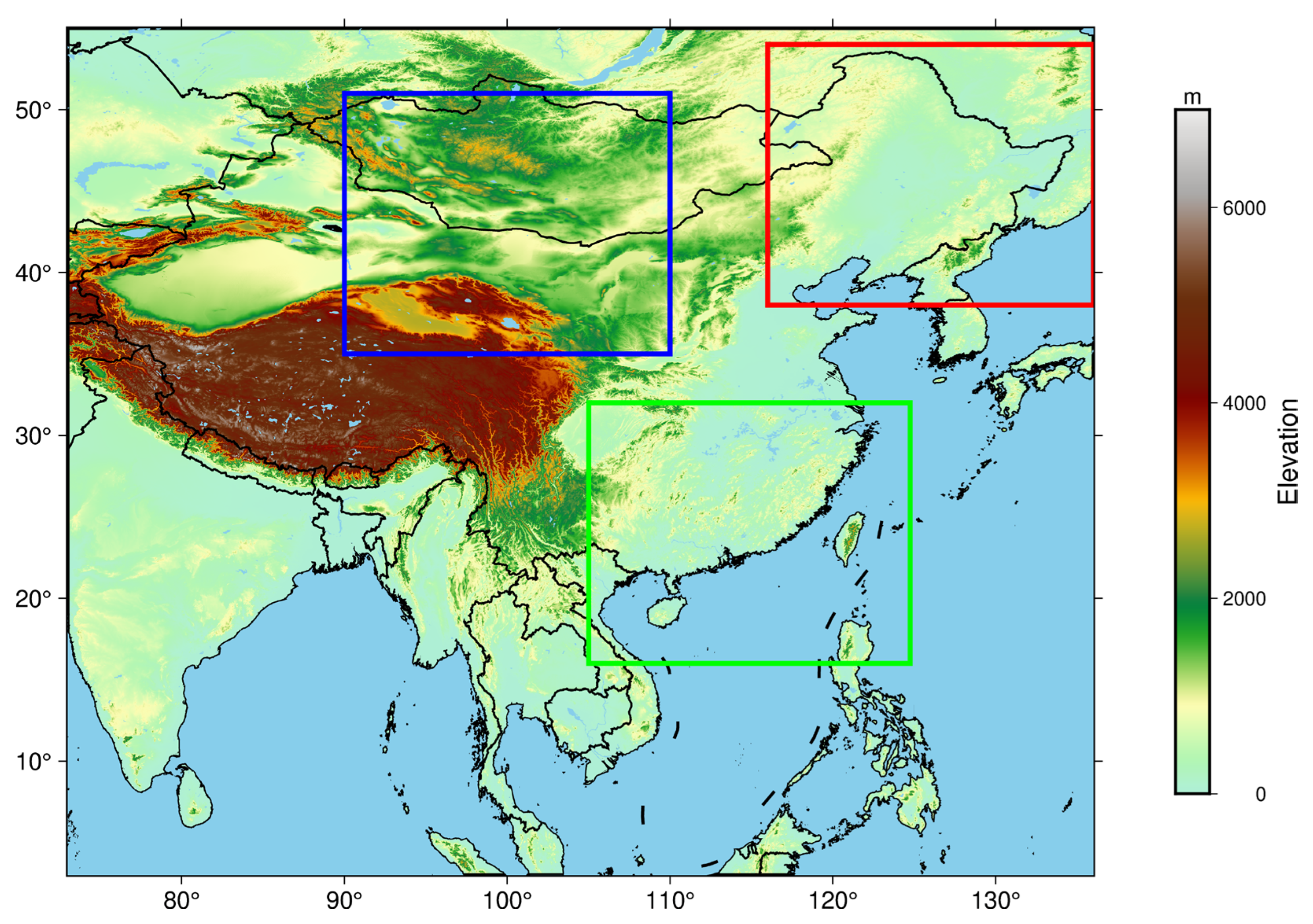
The ERA5 global reanalysis dataset is adopted as the fundamental data source in this study. The zonal and meridional wind components at a height of 100 m are selected as target variables to represent horizontal wind vectors, as this level corresponds to a key layer for wind energy development and atmospheric boundary layer research. Therefore, this study focuses on 100 m wind vector forecasting rather than 10 m station-height wind prediction. To improve model accuracy and generalization capability, geopotential height, air temperature, and elevation are incorporated as auxiliary variables. Geopotential height is used to characterize large-scale circulation patterns, air temperature reflects the modulation effect of thermal structures on wind fields, and elevation is used to describe terrain-induced forcing on near-surface winds. All data are provided at a spatial resolution of 0.25° × 0.25° and a temporal resolution of 1 h, enabling detailed representation of spatiotemporal variations in wind fields. Northeast China [38–54°N, 116–136°E] is selected as the primary experimental region. Northern China and the Mongolian Plateau [35–51°N, 90–110°E], as well as the southeastern coastal area of China and parts of Southeast Asia [16–32°N, 105–125°E], are selected as the transfer experimental regions. These regions are utilized to evaluate model performance and generalization under complex terrain and diverse climatic conditions. As illustrated in Figure 1, the primary experimental region is indicated by the red box, while the blue and green boxes denote the transfer experimental regions. To ensure the objectivity and reproducibility of the results, data from 2018 to 2022 are divided into training and validation sets at a ratio of 9:1, whereas data from 2023 are used as an independent test set for final performance evaluation.

2.3. AMBHFN Framework

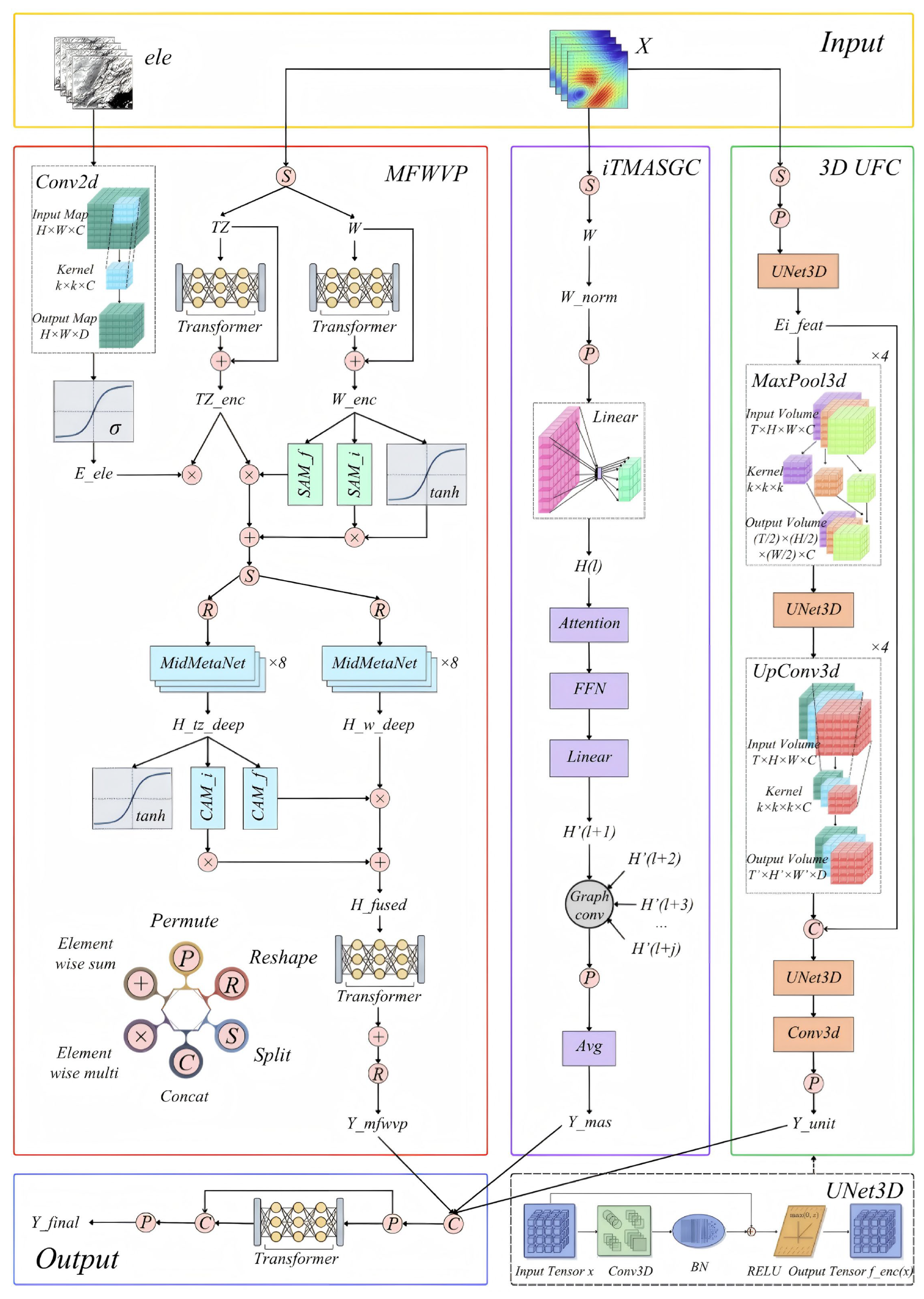
To capture complementary spatiotemporal characteristics of wind fields, a high-precision wind vector prediction model, AMBHFN, is proposed, in which wind vector forecasting is explicitly decomposed into local dynamic modeling, global structural modeling, and temporal robustness modeling. These heterogeneous prediction objectives are assigned to dedicated branches and coordinated through an adaptive fusion mechanism.

Multi-source meteorological variables and terrain information are jointly encoded, thereby enabling short-term wind field variability and multivariate coupling relationships to be effectively characterized through cross-variable spatiotemporal interaction and reconstruction. This branch is designed to emphasize rapid local variations and abrupt wind-field changes. Global spatiotemporal structures are captured by a residual-connected 3D convolutional U-shaped encoder–decoder, in which hierarchical feature extraction and multi-scale reconstruction are employed to maintain a consistent representation of large-scale wind field evolution. Temporal robustness is further enhanced within an iTransformer-based multi-agent framework, in which temporal features are projected into a latent space, refined through graph-based inter-agent interaction, and aggregated to reduce error accumulation during long-horizon prediction.

The prediction outputs generated by MFWVP, 3D UFC, and iTMASGC are first concatenated to form a joint prediction state and are then adaptively coordinated through AMBPC. Through this prediction-level collaboration, complementary information from the three branches is integrated, while local details, global structures, and temporal consistency are jointly preserved in the final wind vector prediction. The overall architecture of AMBHFN is illustrated in Figure 2.

2.4. Referred Modules

2.4.1. Spatial Attention Module

To enhance spatial collaboration across variables, a spatial attention mechanism (SAM) is introduced and defined as follows [38]:

$$SAM\left(X\right)=\sigma \left({Conv}_{7\times 7}\left(\left[{AvgPool}_c\right(X);{MaxPool}_c(X\left)\right]\right)\right)$$

(1)

where ${AvgPool}_c$ and ${MaxPool}_c$ denote channel-wise average pooling and max pooling operations, ${Conv}_{7\times 7}$ denotes a 7 × 7 convolutional layer, and $\sigma$ represents the Sigmoid activation function.

2.4.2. MidMetaNet

To address structural degradation during mid-term wind forecasting, the difficulty in preserving long-range dependencies, and the progressive loss of local details, MidMetaNet is incorporated as a basic operator within the local dynamic branch. By integrating spatial attention with local feature modeling capability, MidMetaNet supports the joint representation of local structure and temporal variation in wind fields. MidMetaNet consists of an eight-layer MetaBlock stack, in which SpatialAttention and MixMLP are alternately combined to capture both long-range dependencies and local details [39].

SpatialAttention is used to model long-range spatial dependencies in wind fields and to highlight key regions such as high-wind-speed zones and terrain convergence belts. Its formulation is given as follows:

$$SpatialAttention\left(X\right)=X+\left[W_2\ast \left(AttentionModule\left(GELU\right(W_1\ast X+b_1\left)\right)\right)+b_2\right]$$

(2)

$MixMLP$ is designed to enhance local feature representation and to compensate for the limitations of spatial attention in local modeling. Its formulation is given as follows:

$$MixMLP\left(X\right)=Drop\left(W_2\ast Drop\left(\sigma \left({DWConv}_{3\times 3}\right(W_1\ast X+b_1\left)\right)\right)\right)+b_2$$

(3)

On this basis, the core update process of $MidMetaNet$ is formulated as follows:

$$H^{l+1}=H^l+DropPath({\gamma }_1\cdot SpatialAttention(Norm(H^l)))$$

(4)

$$H^{l+2}=H^{l+1}+DropPath({\gamma }_2\cdot MixMLP(Norm(H^{l+1})))$$

(5)

The two operations described above are alternately stacked across eight layers, through which spatial and local information are jointly modeled and temporal continuity is maintained.

2.4.3. Channel Attention Mechanism

To adaptively model auxiliary variable correlations and capture intrinsic meteorological dependencies, a channel attention mechanism (CAM) is introduced and defined as follows [38]:

$$CAM(H_{TZ}^{deep})=\sigma \left(MLP(AvgPool(H_{TZ}^{deep}))+MLP(MaxPool(H_{TZ}^{deep}))\right)$$

(6)

where $AvgPool$ and $MaxPool$ denote average pooling and max pooling operations over the spatial dimensions, MLP denotes the shared multilayer perceptron, and σ denotes the Sigmoid activation function.

2.5. Multi-Feature Wind Vector Prediction Branch for Local Dynamic Modeling (MFWVP)

To capture rapid wind-field variations and localized abrupt changes, MFWVP is introduced as the local dynamic branch of AMBHFN. Wind components, auxiliary meteorological variables, and terrain information are decoupled and jointly encoded into a unified spatiotemporal feature space, thereby enhancing the representation of short-term wind variability, cross-variable interactions, and terrain-induced local disturbances.

2.5.1. Multi-Dimensional Meteorological Feature Encoding for Local Dynamics

The input includes raw meteorological data $X_{raw}\in R^{B\times T\times 4\times H\times W}$ and terrain elevation $ele\in R^{H\times W}$. First, $X_{raw}$ is split into wind components $W$ (u, v) and auxiliary variables $TZ$ (temperature and geopotential height at 1000 hPa), while terrain elevation is encoded using a 2D convolution to obtain $E_{ele}\in {\mathbb{R}}^{2\times H\times W}$. This design allows wind-related variables and terrain constraints to be represented separately before local dynamic interaction.

After variable decoupling, the encoder extracts features at each time step using a dual-branch structure. An identity branch preserves local details and produces $X$, while a Transformer branch captures long-range dependencies and produces $X_{se}$. Finally, the two representations are fused through a weighted combination, yielding $X_{enc}$. The fusion weights $w_1$ and $w_2$ are implemented as global learnable scalar parameters and are shared across all channels, spatial locations, and time steps. This process enables local detail preservation and dependency-aware refinement within the same dynamic encoding stage.

Finally, fusion within the encoder is achieved through a gating constraint [40]:

$$W{\prime }_{enc}=(W_{enc}\odot SAM(T{Z}_{enc}\left)\right)+\left(SAM\right(T{Z}_{enc})\odot \tanh (T{Z}_{enc}))+(W_{enc}\odot \sigma \left(E_{ele}\right))$$

(7)

where $\sigma$ denotes the Sigmoid function and $\mathrm{t}\mathrm{a}\mathrm{n}\mathrm{h}$ denotes the hyperbolic tangent activation function.

2.5.2. Cross-Variable Spatiotemporal Interaction for Local Dynamics

To avoid interference between wind components and auxiliary variables, two independent MidMetaNet networks are employed for separate local dynamic modeling. At this stage, the outputs at each time step are reorganized into sequences $H_W=\{W{\prime }_{enc,1},\dots ,W{\prime }_{enc,T}\}$ and $H_{TZ}=\{T{Z}_{enc,1},\dots ,T{Z}_{enc,T}\}$, and are processed by their respective MidMetaNet networks, yielding $H_W^{deep}$ and $H_{TZ}^{deep}$.

Then, channel attention is applied to perform cross-variable fusion, enabling weighted interaction between wind-related and auxiliary features:

$$H_{fused}=\left(H_W^{deep}\odot {CAM}_f(H_T^{deep})\right)+\left({CAM}_i(H_T^{deep})\odot \tanh (H_T^{deep})\right)$$

(8)

2.5.3. Local Dynamic Decoding and Prediction Reconstruction

The high-dimensional feature $H_{fused}$ obtained through cross-variable interaction and fusion is subsequently fed into the decoder. A dual-branch design is retained in the decoder, in which a self-attention branch is employed for dependency modeling and dimensional mapping of the fused features, while an identity mapping branch is introduced to preserve local information and prevent information loss caused by excessive compression. The decoding process is formulated as follows:

Within this dual-branch decoder, a Transformer branch performs dependency-aware modeling and produces $D_{se}$, while an identity branch preserves local information and maintains $D$. Finally, the two representations are fused through a weighted combination, yielding $Y{\prime }_{2D}\in {\mathbb{R}}^{(B·T)\times 2\times H\times W}$. The decoder fusion weights are implemented as global learnable scalars shared across feature channels, spatial locations, and time steps.

Finally, the output is reshaped to restore the spatiotemporal structure and to generate the local dynamic prediction output $Y_{mfiwpn}\in {\mathbb{R}}^{B\times T\times 2\times H\times W}$, which contains the u and v components.

2.6. Three-Dimensional U-Shaped Fully Convolutional Branch for Global Structural Modeling (3D UFC)

To model global spatiotemporal structures and ensure structural consistency across all forecasting horizons, the 3D UFC branch is constructed as the global structural branch of AMBHFN. It is based on a symmetric U-shaped fully convolutional encoder–decoder architecture, in which UNet3DBlock is used as the core unit.

2.6.1. UNet3DBlock for Stable Global Feature Extraction

To address gradient vanishing and insufficient global feature extraction in deep 3D convolutional networks, a residual-connected 3D convolutional unit, UNet3DBlock, is designed as the core module of the global structural branch. The input to the module is a spatiotemporal wind-field feature tensor x. In the main branch, two successive 3 × 3 × 3 3D convolutions, batch normalization (BN), and ReLU activation are performed, and the resulting output is added element-wise to the output of the residual branch, as expressed by:

$$F\left(X\right)=\sigma \left({BN}_2\right(W_2\ast \sigma \left({BN}_1\right(W_1\ast x\left)\right)\left)\right)+Residual\left(x\right)$$

(9)

where $W_1$ and $W_2$ denote 3D convolution weights, ${BN}_1$ and ${BN}_2$ denote batch normalization operations, $\sigma$ denotes the ReLU activation function, and $\ast$ denotes the 3D convolution operation.

The residual branch $Residual\left(x\right)$ adopts a mapping strategy based on the channel consistency between the input and output:

$$r=Residual(x)=\left\{\begin{array}{ll}{W}_{res}\ast x,& if C_{in}\ne C_{out}\\ x,& if C_{in}=C_{out}\end{array}\right.$$

(10)

Here, $W_{res}$ denotes the weight of a 1 × 1 × 1 3D convolution, through which channel alignment is performed when the input and output channels differ, while an identity mapping is directly adopted when they are consistent.

2.6.2. Input Transformation and Global Structural Encoder

The input consists of a 24 h sequence of raw meteorological data $X_{\mathit{raw}}\in R^{B\times T\times C\times H\times W}$, where $C = 4$, corresponding to the four channels $u, v, z$ and $t$. A dimension permutation is first applied to $X_{\mathit{raw}}$ to obtain $X_{3D} = \mathit{Permute}(X_{\mathit{raw}}) \in R^{B\times 4\times T\times H\times W}$. This arrangement treats temporal and spatial dimensions jointly, allowing 3D convolutions to extract continuous spatiotemporal structural features from the 24 h input sequence.

The encoder is composed of four cascaded UNet3DBlock modules, in which structural feature extraction and synchronized spatiotemporal downsampling are performed layer by layer, while multi-scale structural features are preserved [41]:

$$E_{i+1}^{feat}=f_{enc(i+1)}(E_i)\to E_{i+1}=MaxPool3d\left(E_{i+1}^{feat}\right)$$

(11)

Here, $f_{\mathit{enc}}$ denotes the UNet3DBlock operation. At the deepest layer, global structural fusion is performed through a bottleneck module, where the deepest encoded representation $E_4$ is processed to obtain the final fused deep feature $H_{\mathit{deep}}$.

2.6.3. Structural Decoder and Output Mapping

To mitigate the loss of spatial details caused by the encoding process, a symmetric decoder structure is designed to progressively recover wind-field structures through multi-scale feature fusion and to generate the global structural prediction results.

In the decoding stage, 3D transposed convolution $\mathit{UpConv}3d$ is employed for upsampling, and feature maps at corresponding scales preserved by the encoder, $E_i^{\mathit{feat}}, i \in [1,2,3,4]$, are incorporated through concatenation operations $(\parallel )$:

$$D_i=f_{dec\left(i\right)}\left([UpConv3d(H_{deep})\parallel E_i^{feat}]\right)$$

(12)

where $f_{\mathit{dec}}$ denotes the UNet3DBlock operation. In the output stage, a 1 × 1 × 1 3D convolution is first applied to map the feature channels to 2 corresponding to u and v wind components, yielding $Y{\prime }_{3D}={\mathit{Conv}3d}_{1\times 1\times 1}\left(D_1\right) \in R^{B\times 2\times T\times H\times W}$.

Finally, a dimension reordering operation is performed to restore the standard spatiotemporal wind field format, yielding the global structural output $Y_{\mathit{unet}} \in R^{B\times T\times 2\times H\times W}$.

2.7. iTransformer-Based Multi-Agent System with Graph Convolution for Temporal Robustness (iTMASGC)

To improve temporal robustness and reduce error accumulation, iTMASGC is designed as the temporal robustness branch of AMBHFN. Local temporal dynamics are independently modeled by each agent, and inter-agent information exchange is enabled by graph convolution through a learnable inter-agent adjacency matrix. Final outputs are obtained by aggregating the outputs of all agents, thereby reducing error propagation and improving long-horizon stability.

2.7.1. Individual Temporal Perception

In the iTransformer-based multi-agent system, each agent is implemented as an independent temporal model based on the 100 m wind components. First, each variable is normalized along the time dimension to standardize the input data. To mitigate interference from noise in long sequences, the normalized input $X_{norm}$ is first permuted across dimensions and then projected into a latent space through a linear transformation, yielding the initial temporal representation $H^{\left(0\right)}\in R^{B\times C\times d_{model}}$, where the latent dimension is set to $d_{model}=64$ [42,43].

2.7.2. Layer-Wise Temporal Co-Evolution

To model the temporal interaction between the u and v components of wind fields, self-attention is applied across variables. At each layer, the feature update process is as follows:

$$H_{attn}^{(l)}=Attention(H^{(l)}),\hspace{1em}{H}^{(l+1)}=FFN(H_{attn}^{(l)})$$

(13)

Subsequently, a linear projection is performed to map the updated features back to the temporal dimension, producing the reconstructed temporal representation ${\widehat{H}}^{(l+1)}\in R^{B\times C\times T}$.

Local temporal modeling is first performed independently by each agent. After local modeling is completed, temporal features from all agents are fused through graph convolution to facilitate inter-agent information exchange. The inter-agent graph is initialized with a fully connected structure, excluding self-connections, and its edge weights are learned during training. Specifically, a learnable parameter matrix $E\in {\mathbb{R}}^{N\times N}$ is constrained by a Sigmoid function and multiplied by the fully connected structural mask $M$, yielding:

$$A=\sigma \left(E\right)\odot M$$

(14)

The adjacency matrix is then symmetrized as:

$$A_s={\displaystyle \frac{A+A^{\top }}{2}}$$

(15)

Self-loops are added to obtain:

$$\widehat{A}=A_s+I$$

(16)

Finally, degree normalization is performed as:

$$\tilde{A}=D^{-1/2}\widehat{A}{D}^{-1/2},\hspace{1em}{D}_{ii}={\sum }_j{\widehat{A}}_{ij}$$

(17)

The graph convolution operation produces updated representations $X_1^{\left(l\right)},\dots ,X_N^{\left(l\right)}$ from the input features ${\widehat{H}}_1^{\left(l\right)},\dots ,{\widehat{H}}_N^{\left(l\right)}$ and the normalized adjacency matrix $\tilde{A}$, with $X_i^{\left(l\right)}$ denoting the updated representation of agent i. This process enables effective integration of local temporal features and global interaction information.

2.7.3. Individual Temporal Prediction and Collective Decision-Making

Finally, the output features of each agent are transformed back to the physical space through inverse normalization and dimension adjustment. Through this transformation, the dimensionality is restored from $(B,C,T)$ to $(B,T,C)$, and the temporal prediction values $Y_i\in R^{B\times T\times C}$ are obtained. Each iTransformer produces independent predictions, while prediction accuracy varies across regions and datasets. To address this, the predictions from N iTransformer agents are averaged after learnable adjacency-based interaction to obtain the temporal robustness output $Y_{mas}$.

2.8. Adaptive Multi-Branch Prediction Collaboration Mechanism (AMBPC)

In wind vector prediction, the three branches provide functionally complementary prediction mechanisms for modeling local dynamics, global structures, and temporal robustness. MFWVP is effective in short-term forecasting (0–6 h) by modeling local variations and abrupt changes with multi-variable coupling and terrain constraints. Global three-dimensional structural evolution is captured by the 3D UFC, thereby maintaining spatial consistency across all horizons. The iTransformer-based multi-agent system models temporal dynamics and improves long-term forecasting (12–23 h) by enhancing stability and reducing error accumulation. Based on these characteristics, an adaptive prediction collaboration mechanism is designed.

First, prediction outputs from MFWVP, 3D UFC, and iTMASGC are concatenated to obtain a joint prediction state $F_{raw}\in {\mathbb{R}}^{B\times 6\times T\times H\times W}$, after which a dimension permutation is performed to obtain frame-level prediction states $X_t\in {\mathbb{R}}^{B\times 6\times H\times W}$. For each forecast time step, the corresponding state is denoted by $X_t$. To reduce redundancy and coordinate differences among branch predictions, a three-path collaboration module is used. The TransformerBlock path models cross-branch dependencies, the identity path preserves branch-specific predictive information, and the CubeAttention path enhances local cube-wise spatiotemporal interactions. The fused predictive state is computed as:

$$\begin{array}{c}{Z}_t=w_1·\mathrm{T}\mathrm{r}\mathrm{a}\mathrm{n}\mathrm{s}\mathrm{f}\mathrm{o}\mathrm{r}\mathrm{m}\mathrm{e}\mathrm{r}\mathrm{B}\mathrm{l}\mathrm{o}\mathrm{c}\mathrm{k}\left(X_t\right)+w_2·X_t+w_3·\mathrm{C}\mathrm{u}\mathrm{b}\mathrm{e}\mathrm{A}\mathrm{t}\mathrm{t}\mathrm{e}\mathrm{n}\mathrm{t}\mathrm{i}\mathrm{o}\mathrm{n}\left(X_t\right)\end{array}$$

(18)

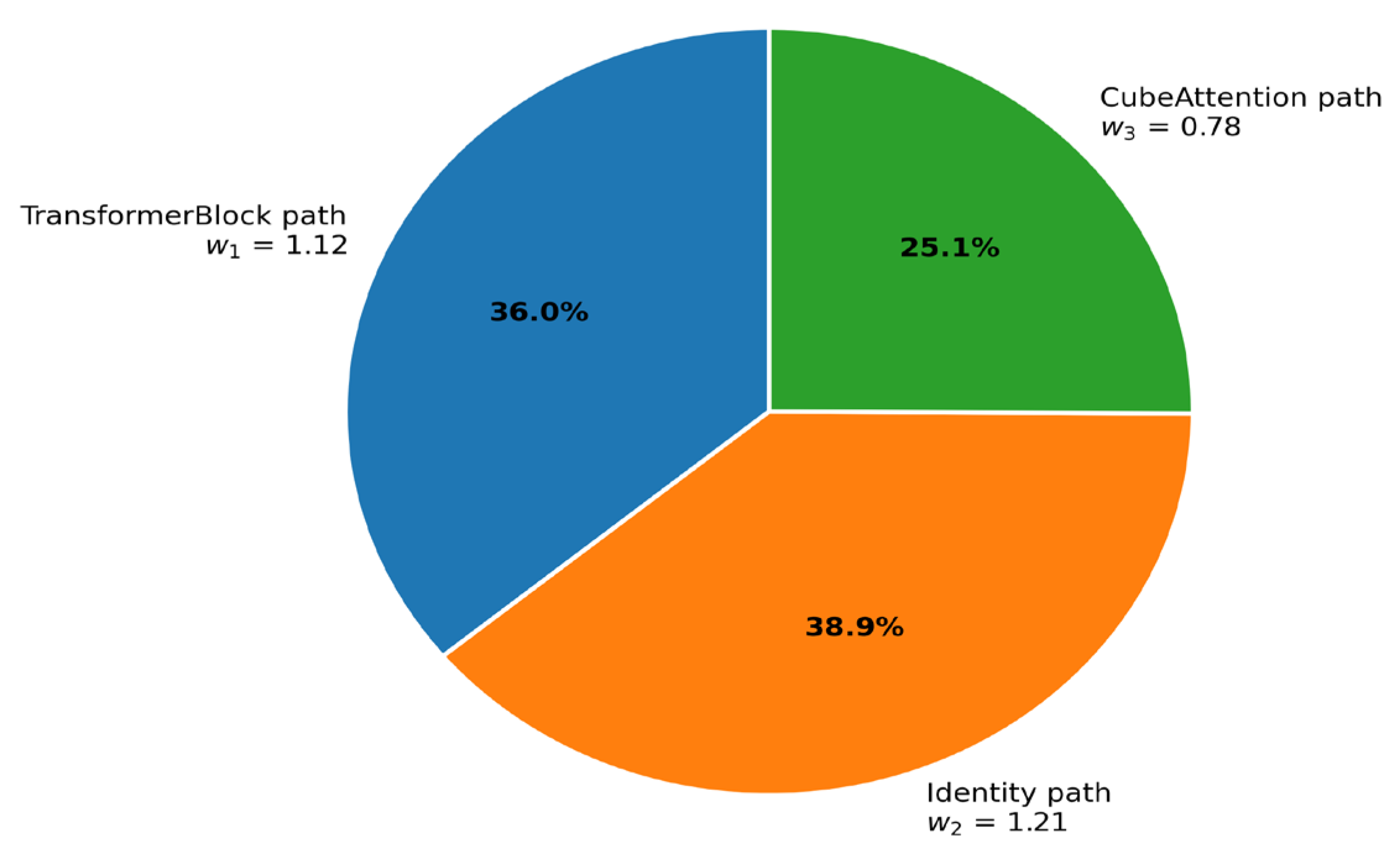
where $w_1$, $w_2$, and $w_3$ are globally learned scalar fusion weights corresponding to the TransformerBlock path, identity path, and CubeAttention path, respectively. They are initialized to 1 and jointly optimized with the entire network through back-propagation during training. Because they are implemented as global scalar parameters, the fusion weights do not vary spatially, temporally, or across feature channels. Instead, the same values are shared across all spatial locations, forecast time steps, and feature channels and are applied to the prediction tensors through broadcasting. After training, the learned scalar weights are $w_1=1.12$, $w_2=1.21$, and $w_3=0.78$, indicating that the identity path has the largest scaling coefficient, followed by the TransformerBlock path and the CubeAttention path. These global scalar weights are shared across spatial locations, forecast time steps, and feature channels, and are applied to the prediction tensors through broadcasting.

After all temporal steps are processed, the predictive states are concatenated again to reconstruct the complete spatiotemporal tensor. Subsequently, a slicing operation is applied to extract the predictive states of the u and v wind components. Finally, a dimension permutation is performed to restore the dimension order of the original input and obtain the final prediction output $Y_{final}\in {\mathbb{R}}^{B\times T\times 2\times H\times W}$. The global scalar fusion weights are expressed as three path-level coefficients, and their learned values are visualized in Figure 3 to improve interpretability. Their sum-normalized relative magnitudes are approximately 36.0%, 38.9%, and 25.1% for the TransformerBlock, identity, and CubeAttention paths, respectively. These values represent the relative scaling strengths of the three collaboration paths and should be interpreted as path-level scaling coefficients.

2.9. Evaluation Metrics

Due to the spherical nature of the Earth, latitude–longitude grids introduce a spatial imbalance because grid cells at higher latitudes represent smaller physical areas than those near the equator. To correct this geometric bias, a latitude-dependent weight is introduced as follows:

$$w(h)={\displaystyle \frac{\cos ({\theta }_h)}{\frac{1}{H}{\sum }_{j=1}^H\cos ({\theta }_j)}}$$

(19)

Based on this spatial weighting, RMSE, MAE, and ACC are formulated to better reflect the true geophysical distribution of errors. The weighted RMSE is computed by first weighting the squared errors across all samples and spatial grid cells, after which a global square root is taken:

$$RMS{E}_t=\sqrt{{\displaystyle \frac{{\sum }_{b=1}^B{\sum }_{h=1}^H{\sum }_{\mathcal{l}=1}^{W}w(h)({\widehat{y}}_{b,t,h,\mathcal{l}}-y_{b,t,h,\mathcal{l}}{)}^2}{B·W·{\sum }_{h=1}^{H}w(h)}}}$$

(20)

Similarly, the weighted MAE measures the weighted average absolute deviation under the same spatial correction:

$$MA{E}_t={\displaystyle \frac{{\sum }_{b=1}^B{\sum }_{h=1}^H{\sum }_{\mathcal{l}=1}^{W}w(h)|{\widehat{y}}_{b,t,h,\mathcal{l}}-y_{b,t,h,\mathcal{l}}|}{B·W·{\sum }_{h=1}^{H}w(h)}}$$

(21)

ACC measures the spatially weighted correlation between predicted and observed anomalies, thereby allowing correlation consistency to be evaluated without latitude-induced distortion:

$$AC{C}_t={\displaystyle \frac{{\sum }_{b=1}^B{\sum }_{h=1}^H{\sum }_{\mathcal{l}=1}^{W}w(h)({\widehat{y}\prime }_{b,t,h,\mathcal{l}}-{\mu }_{\widehat{y}\prime })({\mathrm{y}\prime }_{b,t,h,\mathcal{l}}-{\mu }_{y\prime })}{\sqrt{{\sum }_{b=1}^B{\sum }_{h=1}^H{\sum }_{\mathcal{l}=1}^{W}w(h)({\widehat{y}\prime }_{b,t,h,\mathcal{l}}-{\mu }_{\widehat{y}\prime }{)}^2}\sqrt{{\sum }_{b=1}^B{\sum }_{h=1}^H{\sum }_{\mathcal{l}=1}^{W}w(h)({\mathrm{y}\prime }_{b,t,h,\mathcal{l}}-{\mu }_{y\prime }{)}^2}}}$$

(22)

where $\widehat{y}\prime$ and $y\prime$ denote the predicted and observed anomalies, and ${\mu }_{\widehat{y}\prime }$ and ${\mu }_{y\prime }$ denote their corresponding means. For wind direction evaluation, the wind direction angle is computed using $\theta =atan2(v,u)$. To assess prediction accuracy under different directional accuracy requirements, three tolerance thresholds are defined: $\alpha \in \{90^{\circ },45^{\circ },22.5^{\circ }\}$. A prediction is considered correct if the circular angular deviation does not exceed the specified threshold:

$$WDF{A}_{t,\alpha }={\displaystyle \frac{1}{N}}{\displaystyle \sum _{i=1}^N}\mathrm{I}\left(\min \left(\left|{\widehat{\theta }}_i-{\theta }_i\right|,360^{\circ }-\left|{\widehat{\theta }}_i-{\theta }_i\right|\right)\le \alpha \right)\times 100\%$$

(23)

This multi-level threshold design enables a more comprehensive evaluation of directional prediction accuracy under both relaxed and strict conditions.

3. Results

3.1. Comprehensive Performance Analysis

A comprehensive benchmarking system covering mainstream wind vector prediction methods is constructed to systematically evaluate the proposed model under a multi-dimensional metric framework. Baseline models are organized according to the development trajectory of spatiotemporal prediction methods to ensure completeness and rigor. TCN is used as a temporal convolutional baseline to capture long-range temporal dependencies through causal convolutions [44]. As a representative spatiotemporal framework, ConvLSTM jointly models the spatial structure and temporal evolution of wind fields [22]. E3DLSTM combines 3D convolution with memory mechanisms to enhance the modeling of short-term spatiotemporal dynamics [23]. MMVP models temporal dynamics via motion matrices and is suited for strongly nonlinear wind fields [45]. TAU introduces adaptive temporal attention to capture both short- and long-term dependencies and reduce error accumulation in long-horizon forecasting [46]. TropiCycloneNet incorporates physical priors into data-driven learning for meteorology-oriented modeling [41]. STDGN uses decoupled attention to model complex multivariate spatiotemporal dependencies [47]. MFWPN is further included as a strong multivariate fusion baseline aligned with practical engineering scenarios [39]. All baseline results reported in this study are obtained by retraining the corresponding models using the same dataset and under the same input–output, normalization, training, and evaluation settings as those used for AMBHFN.

The experiments are conducted under a twice-daily forecasting scheme with initialization times of 00:00 and 12:00, in which each sample uses the preceding 24 h meteorological sequence as input and each run directly produces wind vector predictions for the subsequent 24 h. For AMBHFN and all baseline models, the same ERA5 dataset, study region, 2018–2022 training/validation split, 2023 test set, normalization strategy, and 24 h input–24 h output setting are used. For AMBHFN and each baseline model, five independent runs are conducted with different random seeds under the same experimental protocol, and the best-performing checkpoint is selected based on validation-set performance for final test evaluation and reporting. The results are presented in

Table 2. RMSE results for different models.

Models	0 h	1 h	2 h	3 h	4–6 h	7–12 h	13–23 h
TCN	0.50	0.77	0.98	1.17	1.45	1.98	2.67
ConvLSTM	0.58	0.94	1.20	1.39	1.64	1.96	2.41
E3DLSTM	0.66	0.91	1.12	1.30	1.60	2.16	2.76
MMVP	1.91	1.92	1.93	1.95	1.98	2.01	2.26
TAU	0.48	0.73	0.91	1.04	1.26	1.65	2.20
TropiCycloneNet	0.53	0.67	0.81	0.93	1.12	1.50	2.07
STDGN	0.44	0.73	0.94	1.10	1.36	1.79	2.33
MFWPN	0.42	0.66	0.83	0.96	1.16	1.55	2.13
AMBHFN	0.33	0.57	0.74	0.86	1.06	1.42	1.94

,

Table 3. MAE results for different models.

Models	0 h	1 h	2 h	3 h	4–6 h	7–12 h	13–23 h
TCN	0.39	0.59	0.75	0.89	1.11	1.53	2.11
ConvLSTM	0.44	0.73	0.93	1.08	1.27	1.52	1.88
E3DLSTM	0.49	0.70	0.86	0.99	1.23	1.66	2.15
MMVP	1.47	1.48	1.49	1.50	1.53	1.57	1.77
TAU	0.37	0.56	0.69	0.80	0.96	1.25	1.70
TropiCycloneNet	0.40	0.51	0.61	0.70	0.84	1.13	1.61
STDGN	0.33	0.55	0.72	0.84	1.03	1.36	1.79
MFWPN	0.32	0.51	0.64	0.73	0.88	1.17	1.64
AMBHFN	0.25	0.43	0.56	0.65	0.80	1.06	1.49

and

Table 4. ACC results for different models.

Models	0 h	1 h	2 h	3 h	4–6 h	7–12 h	13–23 h
TCN	0.98	0.94	0.91	0.87	0.81	0.64	0.39
ConvLSTM	0.98	0.94	0.90	0.87	0.83	0.73	0.58
E3DLSTM	0.97	0.94	0.91	0.88	0.83	0.66	0.44
MMVP	0.68	0.67	0.66	0.65	0.63	0.61	0.51
TAU	0.98	0.96	0.94	0.92	0.89	0.79	0.63
TropiCycloneNet	0.98	0.96	0.94	0.92	0.88	0.78	0.62
STDGN	0.99	0.96	0.94	0.92	0.88	0.77	0.59
MFWPN	0.99	0.97	0.94	0.93	0.89	0.80	0.63
AMBHFN	0.99	0.97	0.95	0.93	0.90	0.81	0.64

, with the values in Table 2 and Table 3 reported in m/s. The evaluation metrics include RMSE, MAE, and ACC. RMSE is used to evaluate prediction errors with greater sensitivity to large deviations, MAE reflects the overall deviation level, and ACC measures the anomaly correlation between predictions and observations. Based on this metric system, the predictive performance of different models is systematically compared across multiple evaluation dimensions.

In Table 2, Table 3 and Table 4, the labels from 0 to 23 h denote the forecast lead times within the direct 24 h output sequence, with 0 h corresponding to the first-step prediction based on the preceding 24 h input sequence. The reported values are obtained by averaging the two daily forecasts initialized at 00:00 and 12:00. AMBHFN is compared with TCN, ConvLSTM, E3DLSTM, MMVP, TAU, TropiCycloneNet, STDGN, and MFWPN using RMSE, MAE, and ACC across the full forecasting horizon. Classical models such as TCN, ConvLSTM, and E3DLSTM exhibit clear performance degradation with increasing lead time, with larger errors and lower ACC at longer forecast lead times. MMVP performs the worst overall, exhibiting consistently high errors. TropiCycloneNet shows moderate improvement but still exhibits noticeable error growth. TAU and STDGN achieve more stable results, while MFWPN provides the strongest baseline with relatively balanced accuracy and stability among existing methods.

In contrast, AMBHFN achieves the lowest errors across most lead times and maintains competitive ACC over both short- and long-term forecast horizons, with only limited degradation as the forecast horizon increases. Compared with MFWPN, AMBHFN achieves lower weighted RMSE and MAE and higher ACC. As shown in

Table 5. Weighted paired statistical test results between AMBHFN and MFWPN.

Metric	t-Test p	Wilcoxon p	95% CI	Significant
RMSE	0.000001	0.000014	[−0.1630, −0.1320]	✓
MAE	0.000001	0.000013	[−0.1307, −0.1076]	✓
ACC	0.000003	0.000005	[0.0076, 0.0112]	✓
WDFA 90°	0.000001	0.000035	[0.1464, 0.1661]	✓
WDFA 45°	0.000001	0.000017	[0.1437, 0.1538]	✓
WDFA 22.5°	0.000001	0.000018	[0.6961, 0.7589]	✓

, both the paired t-tests and Wilcoxon signed-rank tests indicate statistically significant improvements in weighted RMSE, MAE, and ACC, with all p-values below 0.001 and all 95% confidence intervals excluding zero. Although the ACC improvement is smaller in magnitude, it remains statistically significant. These results indicate enhanced spatiotemporal modeling capability and stable temporal performance throughout the forecast horizon.

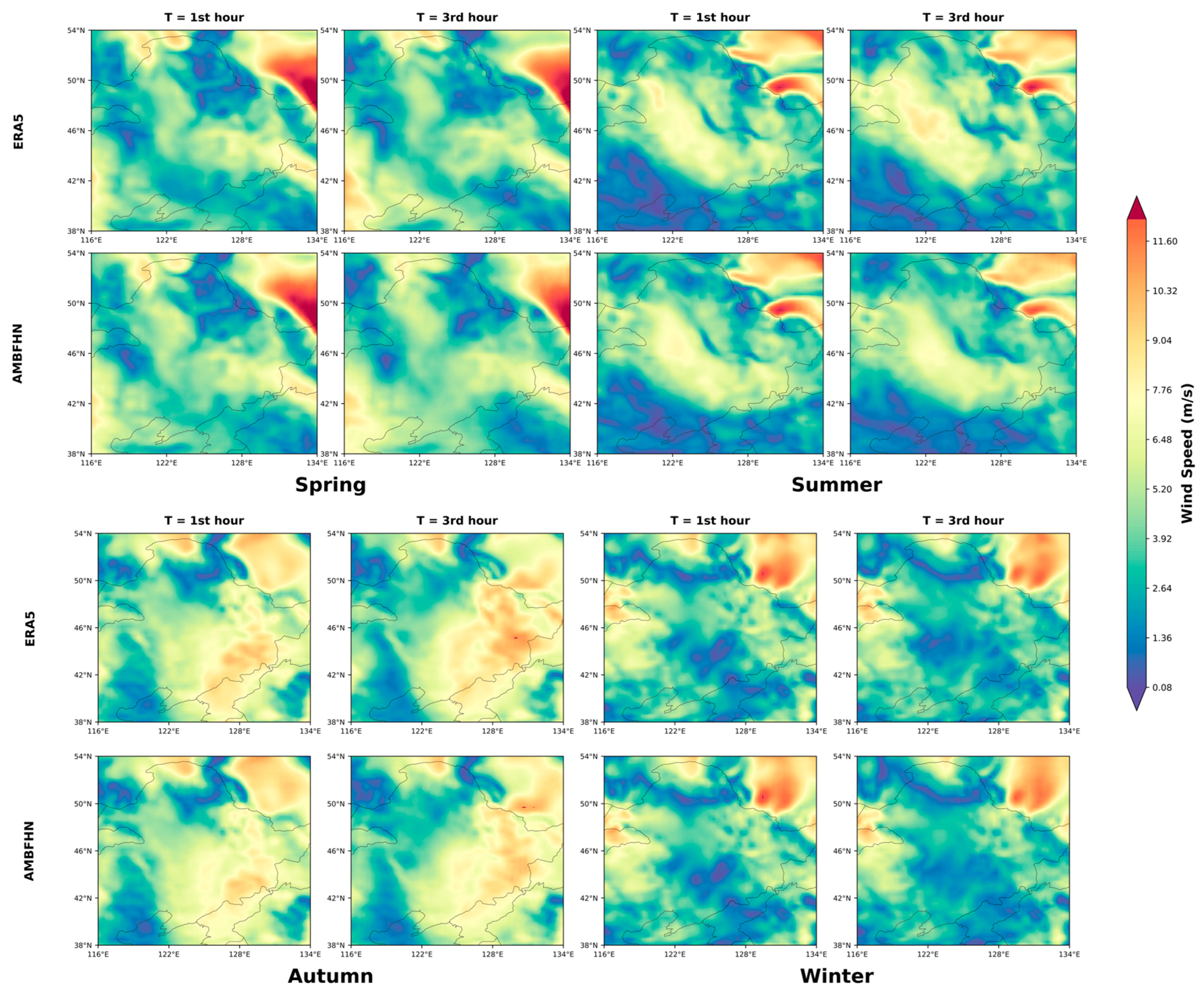
Figure 4 compares spatial wind speed distributions over Northeast China in 2023 across four seasons for the 1 h and 3 h lead times. AMBHFN predictions show a high degree of spatial consistency with ERA5 observations, with dominant wind patterns and high-wind-speed regions well reconstructed in all seasons. In spring and summer, high-wind-speed bands and their local gradients are accurately captured, and clear spatial structures are maintained at 3 h. In autumn, large-scale transition zones are reproduced, with spatial evolution trends consistent with observations. In winter, despite more heterogeneous conditions, the relative distribution of low- and high-wind-speed regions is preserved. These results indicate strong structural preservation and cross-season generalization capability. This performance is enabled by collaborative modeling across the three branches through adaptive multi-branch fusion.

Table 6. WDFA results of different models for wind direction prediction.

Models	0 h (%)			3 h (%)			6 h (%)			12 h (%)
	α = 90	α = 45	α = 22.5	α = 90	α = 45	α = 22.5	α = 90	α = 45	α = 22.5	α = 90	α = 45	α = 22.5
TCN	99.61	98.61	95.19	97.53	91.79	77.27	95.12	85.02	65.20	87.46	69.87	47.21
ConvLSTM	99.58	98.49	94.86	97.29	90.74	74.05	95.47	85.39	64.41	91.52	76.77	53.62
E3DLSTM	99.44	97.98	93.23	97.29	91.10	75.85	94.51	83.83	63.31	86.23	67.54	44.24
MMVP	90.29	75.95	54.58	89.96	75.18	54.04	89.69	74.45	53.85	87.96	71.42	49.34
TAU	99.72	98.97	96.40	98.37	94.41	83.04	96.97	90.38	74.74	92.97	81.00	60.74
TropiCycloneNet	99.44	98.08	93.80	98.11	93.86	82.91	96.52	89.53	74.63	92.54	81.68	62.95
STDGN	99.75	99.09	96.80	98.18	93.80	81.56	96.52	88.93	71.82	92.14	78.62	56.74
MFWPN	99.80	99.22	97.31	98.38	94.92	84.96	97.19	91.08	76.64	93.12	81.84	63.17
AMBHFN	99.82	99.36	97.72	98.50	94.95	85.18	97.33	91.58	78.06	93.16	81.90	63.23

compares the wind direction prediction performance of AMBHFN with that of eight comparison models at lead times of 0 h, 3 h, 6 h, and 12 h. WDFA is used as the evaluation metric under three tolerance thresholds of 90°, 45°, and 22.5°, with smaller thresholds corresponding to stricter accuracy requirements. Results show that AMBHFN achieves optimal or near-optimal WDFA values across most lead times and thresholds. At 0 h, WDFA reaches 99.82%, 99.36%, and 97.72% under the three thresholds, with a gain of 0.41 percentage points over MFWPN under the strictest threshold. At 3 h, the gain over MFWPN under the 22.5° threshold is 0.22 percentage points. At 6 h, WDFA under 22.5° reaches 78.06%, exceeding MFWPN by 1.42 percentage points. At 12 h, AMBHFN reaches 63.23% under the strict threshold, exceeding MFWPN by 0.06 percentage points. Although this horizon-specific gain is small in magnitude, the weighted paired statistical analysis in Table 6 confirms that the overall WDFA improvement under the 22.5° threshold is statistically significant.

Overall, AMBHFN exhibits more gradual performance degradation over 0–12 h and maintains competitive stability in long-term wind direction prediction under strict accuracy requirements. As shown in Table 6, the paired t-tests and Wilcoxon signed-rank tests demonstrate statistically significant overall WDFA improvements under the 90°, 45°, and 22.5° thresholds. Although the gains under the 90° and 45° thresholds are small in magnitude, they remain statistically significant. This advantage is supported by the stable structural representation provided by UNet3DBlock and the effective error control achieved through prediction-level adaptive multi-branch fusion.

To determine whether the numerical improvements over the strongest baseline are statistically significant, paired statistical tests are conducted between AMBHFN and MFWPN based on matched test samples. For each metric, the paired difference is defined as $d_i=m_i^{AMBHFN}-m_i^{MFWPN}$, where $i$ denotes the matched test case. For RMSE and MAE, negative differences indicate lower errors for AMBHFN, while for ACC and WDFA, positive differences indicate higher accuracy. The paired t-test is used to determine whether the mean paired difference is significantly different from zero, and its statistic is computed as:

$$t={\displaystyle \frac{\overline{d}}{s_d/\sqrt{n}}}$$

(24)

where $\overline{d}$ and $s_d$ denote the mean and standard deviation of the paired differences, and the corresponding p-value is reported as $p_t$. The Wilcoxon signed-rank test is further applied to the nonzero paired differences as a nonparametric counterpart. After the absolute differences $\left|d_i\right|$ are ranked, the positive and negative rank sums are denoted by $W^{+}$ and $W^{-}$, and the test statistic is defined as:

$$W=\min (W^{+},W^{-})$$

(25)

The corresponding Wilcoxon p-value is reported as $p_W$. In addition, the 95% confidence interval is obtained by bootstrap resampling of ${d_i}_{i=1}^n$. Based on $B$ bootstrap-resampled mean differences ${\overline{d}}^{\ast \left(b\right)}$, the confidence interval is computed as:

$$C{I}_{95\%}=\left[Q_{2.5\%}({\overline{d}}^{\ast }),Q_{97.5\%}({\overline{d}}^{\ast })\right]$$

(26)

As shown in Table 5, both the paired t-test and the Wilcoxon signed-rank test yield p-values below 0.001 for all six reported metrics, and all 95% confidence intervals exclude zero. These results confirm that AMBHFN achieves statistically significant improvements over MFWPN in weighted RMSE, MAE, ACC, WDFA under the 90° threshold, WDFA under the 45° threshold, and WDFA under the 22.5° threshold. The WDFA gains under the 90° and 45° thresholds are statistically significant but small in magnitude.

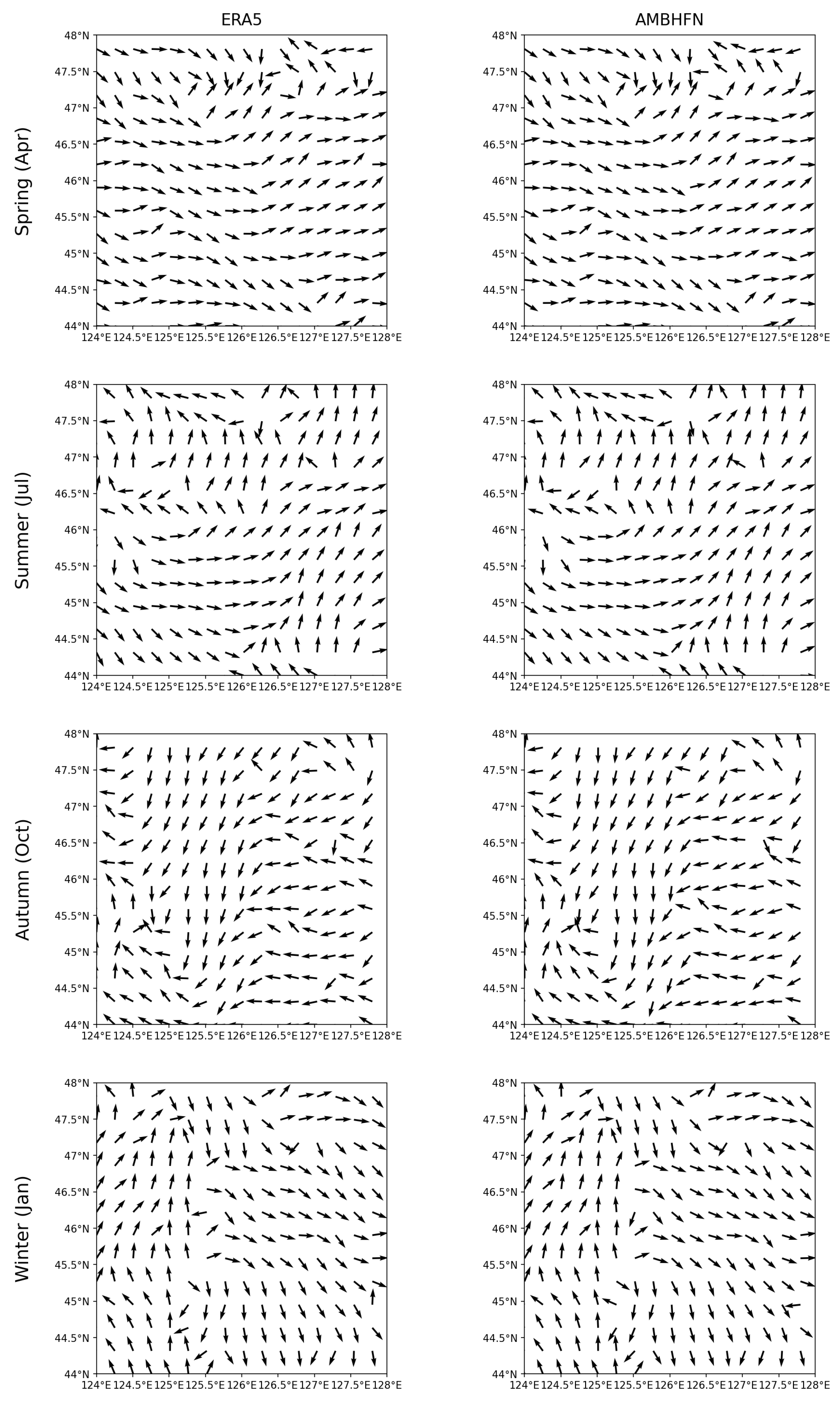
Figure 5 compares ERA5 observations with AMBHFN predictions of seasonal wind direction fields to evaluate model performance across representative flow structures. The arrows in Figure 5 indicate the wind directions. In spring, both ERA5 and AMBHFN exhibit a westerly-dominated flow from west to east in the central region, with local disturbances and rotational features near 47.5°N in the north being accurately reproduced. In summer, ERA5 shows southerly flow in the eastern region around 127°E and prevailing westerlies in the central region, and this combined pattern is effectively captured by AMBHFN. In autumn, a dominant northerly-to-easterly flow and a central divergent structure are observed in ERA5, which are consistently reproduced in terms of both directional distribution and spatial expansion. In winter, ERA5 presents strong northward transport in the western region around 125°E and northwesterly flow in the southeast, which are also well captured by the model.

Overall, dominant wind directions, regional circulation structures, and key local features are consistently reconstructed across seasons, indicating strong structural preservation under complex terrain and cross-season conditions. This performance is attributed to the collaborative modeling performed across the three parallel branches.

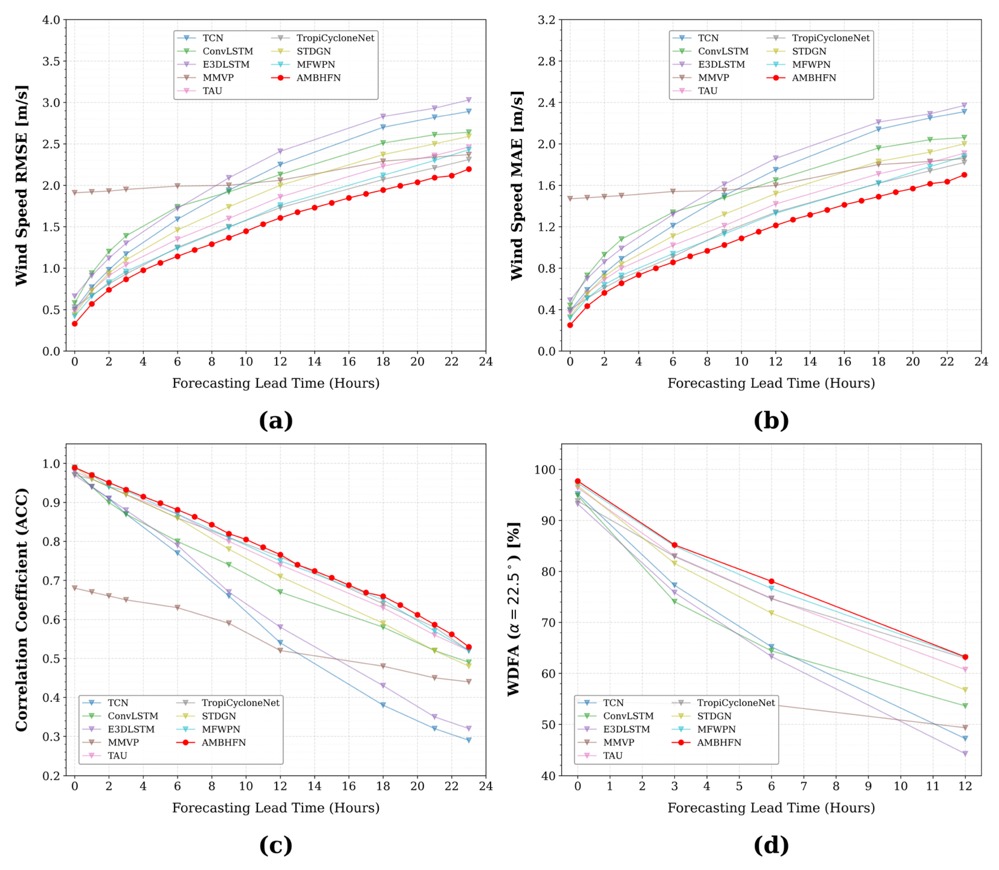
Figure 6a–d compares the performance of different models over the 24 h prediction window, corresponding to 0–23 h forecast lead times, using RMSE, MAE, ACC, and WDFA. With increasing lead time, all models exhibit progressive error accumulation, characterized by rising RMSE and MAE and declining ACC and WDFA, which reflects the typical performance degradation observed in long-horizon forecasting.

In contrast, AMBHFN achieves competitive or near-optimal performance across the evaluated metrics. RMSE and MAE remain at relatively low levels throughout the forecasting range and increase more slowly, indicating improved control of error accumulation. The ACC curve shows a relatively slow decline, indicating that the temporal consistency of wind field structures is preserved, while WDFA remains competitive among the compared models. Compared with TCN, ConvLSTM, and E3DLSTM, which exhibit pronounced performance degradation at longer forecast lead times, AMBHFN demonstrates stable temporal performance, supporting the effectiveness of the model in spatiotemporal wind field modeling and error control.

3.2. Auxiliary Analysis of Multi-Horizon Stability and Consistency

Traditional metrics such as RMSE, MAE, and ACC are mainly used to evaluate prediction accuracy at individual forecast horizons, but their absolute values cannot fully reflect model stability across multiple forecast horizons. This limitation is more evident for wind fields with strong nonlinearity and complex spatiotemporal dynamics, for which both accuracy and temporal stability are critical. To provide an auxiliary description of multi-horizon behavior, prediction errors are treated as a time-evolving process, and four descriptive indicators are used: Standard Deviation, Error Growth Rate, Robustness Index, and Metric Consistency. The Robustness Index serves as an auxiliary summary of temporal fluctuation and error growth, while established uncertainty and probabilistic reliability metrics remain the primary tools for formal reliability assessment.

Standard Deviation (Std) is used to measure temporal stability across different forecast lead times by quantifying the dispersion of RMSE, MAE, and ACC over time. A smaller value indicates more stable performance, while a larger value reflects stronger fluctuation. For RMSE, the standard deviation is defined as follows:

$${\sigma }_{RMSE}=\sqrt{{\displaystyle \frac{1}{T}}{\displaystyle \sum _{t=1}^T}(RMSE(t)-\overline{RMSE}{)}^2}$$

(27)

Similarly, ${\sigma }_{MAE}$ and ${\sigma }_{ACC}$ are defined in the same manner.

Error Growth Rate (Growth) measures the average absolute change between adjacent forecast lead times, describing how RMSE, MAE, and ACC evolve across the forecast horizon. Smaller values indicate smoother error variation and better multi-step stability, while larger values imply faster error propagation. For RMSE, the error growth rate is defined as follows:

$$G_{RMSE}={\displaystyle \frac{1}{T-1}}{\displaystyle \sum _{t=1}^{T-1}}\left|RMSE(t+1)-RMSE\left(t\right)\right|$$

(28)

Similarly, $G_{MAE}$ and $G_{ACC}$ are defined in the same manner. To better distinguish differences among models in $G_{ACC}$, all $G_{ACC}$ values are scaled by a factor of 100.

The Robustness Index is used as an auxiliary summary of temporal fluctuation and error growth and is constructed by inversely weighting Standard Deviation and Error Growth Rate. To avoid instability when the denominator approaches zero, a small constant ε is introduced:

$$R{I}_m=\alpha {\displaystyle \frac{1}{St{d}_m+\epsilon }}+\beta {\displaystyle \frac{1}{Growt{h}_m+\epsilon }},\hspace{1em}m\in RMSE,MAE,ACC$$

(29)

where $\alpha$ and $\beta$ denote weighting coefficients, and $\epsilon =10^{-6}$ is used for numerical stability. In this study, $\alpha =\beta =0.5$ is adopted because no prior assumption is made regarding whether temporal fluctuation is more important than error growth, or vice versa; therefore, both terms are assigned equal importance. To examine sensitivity to this choice, additional calculations are performed with $(\alpha ,\beta )=(0.3, 0.7)$, $(0.5, 0.5)$, and $(0.7, 0.3)$. The ranking of AMBHFN remains unchanged for RMSE-, MAE-, and ACC-based RI under these settings, indicating that the auxiliary RI comparison is not sensitive to moderate changes in $\alpha$ and $\beta$. Because RI depends on the selected weighting coefficients, it is interpreted jointly with the separate Std and Growth values and is used as an auxiliary stability indicator.

Metric Consistency (MC) evaluates the agreement among RMSE, MAE, and ACC by summing their variances, thereby avoiding over-reliance on a single metric. A smaller value indicates more consistent behavior across metrics and provides an auxiliary indication of metric-level stability. The metric is defined as follows:

$$C=Var\left(RMSE\right)+Var\left(MAE\right)+Var\left(ACC\right)$$

(30)

As shown in

Table 7. Auxiliary benchmarking of multi-horizon stability and consistency for different models.

Models	Std			Growth			Robustness Index			MC
	RMSE	MAE	ACC	RMSE	MAE	ACC	RMSE	MAE	ACC
TCN	0.84	0.68	0.25	0.27	0.21	7.67	2.48	3.08	8.49	1.24
ConvLSTM	0.69	0.54	0.17	0.23	0.18	5.44	2.91	3.70	12.15	0.79
E3DLSTM	0.84	0.66	0.24	0.26	0.21	7.22	2.50	3.15	9.02	1.20
TAU	0.67	0.52	0.16	0.22	0.17	5.15	3.01	3.88	12.86	0.75
STDGN	0.73	0.57	0.18	0.24	0.19	5.67	2.78	3.58	11.59	0.89
MFWPN	0.68	0.52	0.16	0.22	0.17	5.22	2.98	3.84	12.66	0.76
AMBHFN	0.63	0.49	0.15	0.21	0.16	5.11	3.21	4.13	12.95	0.66

, AMBHFN obtains favorable auxiliary stability and consistency values among all compared models. It achieves the lowest Std values of 0.63, 0.49, and 0.15 as well as the lowest Growth values of 0.21 and 0.16, indicating smaller temporal fluctuations and slower error accumulation in this evaluation setting. In Table 5, the Robustness Index is calculated under the equal-weight setting of $(\alpha ,\beta )=(0.5, 0.5)$. The Robustness Index reaches 12.95 and serves as an auxiliary summary consistent with the separate Std and Growth results. In terms of consistency, AMBHFN achieves the lowest Metric Consistency value of 0.66, showing better agreement among RMSE, MAE, and ACC, while other models exhibit larger variations across metrics. Overall, these results indicate more stable multi-horizon behavior in this evaluation setting. The separate Std and Growth trends provide the primary evidence, while RI serves as a complementary summary indicator.

Overall, these results suggest that AMBHFN exhibits more stable multi-horizon behavior and greater metric consistency than the compared baseline models in this evaluation setting.

3.3. Transfer Experiments

After AMBHFN is validated in northeastern China, cross-regional transfer experiments are conducted in the northern China and Mongolian Plateau region [35–51°N, 90–110°E] and the Southeast Asian and southeastern coastal region [16–32°N, 105–125°E] to further evaluate its generalization and robustness beyond the independent evaluation conducted on the 2023 test set. The two regions differ markedly in climate regimes and terrain conditions, providing complementary evidence for model performance under domain shifts. A model pretrained using data from northeastern China is used, and fine-tuning is performed using ERA5 data from each target transfer region. To evaluate adaptation efficiency, fine-tuning is conducted for only 10 epochs while keeping the overall model architecture unchanged. These fine-tuning data are prepared using the same variable format, temporal span, training/validation/test split, normalization strategy, and 24 h input–24 h output setting as those used for the primary experimental region, with only the geographic region changed to isolate the effect of domain shift. Therefore, the transfer experiments serve as an additional generalization assessment across heterogeneous climatic and geographic conditions, complementing the single-year temporal test in the source region.

As shown in

Table 8. RMSE, MAE, and ACC results comparison of AMBHFN before and after fine-tuning in the Southeastern Coastal China–Southeast Asia region and the Northern China–Mongolian Plateau region.

Models	0 h			1 h			2 h			3 h			4–6 h			7–12 h			13–23 h
	RMSE	MAE	ACC	RMSE	MAE	ACC	RMSE	MAE	ACC	RMSE	MAE	ACC	RMSE	MAE	ACC	RMSE	MAE	ACC	RMSE	MAE	ACC
South-Pre	0.43	0.34	0.99	0.95	0.76	0.95	1.37	1.09	0.89	1.67	1.33	0.84	2.07	1.62	0.74	2.55	1.96	0.53	3.11	2.39	0.30
South-Finetuned	0.35	0.26	0.99	0.56	0.42	0.97	0.70	0.53	0.96	0.81	0.61	0.95	0.96	0.72	0.93	1.19	0.88	0.88	1.54	1.13	0.79
North-Pre	0.47	0.33	0.98	1.08	0.81	0.94	1.57	1.19	0.87	1.95	1.48	0.79	2.42	1.84	0.65	2.89	2.21	0.46	3.27	2.51	0.31
North-Finetuned	0.34	0.26	0.99	0.58	0.44	0.97	0.76	0.56	0.95	0.86	0.67	0.93	1.06	0.82	0.89	1.45	1.07	0.80	1.96	1.49	0.64

, both regions exhibit clear degradation in generalization performance before fine-tuning, with rapid error accumulation and structural deterioration as forecast lead time increases. In the Southeast Asian and southeastern coastal region, RMSE rises from 0.43 to 3.11 while ACC drops from 0.99 to 0.30. In the northern China and Mongolian Plateau region, RMSE increases from 0.47 to 3.27 and ACC decreases from 0.98 to 0.31, indicating strong domain shift effects.

After fine-tuning, this trend is effectively mitigated. Over the 13–23 h forecast range, RMSE decreases to 1.54 and 1.96, while ACC recovers to 0.79 and 0.64, respectively, indicating greater dynamical consistency and improved preservation of large-scale structures.

Table 9. WDFA results comparison of AMBHFN before and after fine-tuning in the Southeastern Coastal China–Southeast Asia region and the Northern China–Mongolian Plateau region.

Models		0 h (%)			3 h (%)			6 h (%)			12 h (%)
	α = 90	α = 45	α = 22.5	α = 90	α = 45	α = 22.5	α = 90	α = 45	α = 22.5	α = 90	α = 45	α = 22.5
South-Pre	99.67	98.82	95.70	96.00	86.78	67.63	92.36	77.77	54.14	80.70	57.07	33.76
South-Finetuned	99.78	99.20	97.01	99.00	96.26	87.40	98.48	94.47	82.94	96.92	89.88	74.08
North-Pre	99.34	98.74	93.97	95.77	85.15	66.59	92.16	77.56	54.05	80.36	56.12	32.46
North-Finetuned	99.80	99.26	97.22	98.46	94.87	85.13	97.25	91.50	77.91	93.01	81.78	63.06

North: Northern China and Mongolian Plateau region; South: Southeast Asia and southeastern coastal China; Pre: before fine-tuning; Finetuned: after fine-tuning.

further shows that fine-tuning consistently improves WDFA across all thresholds and forecast lead times in both regions. Under the strict $\alpha =22.5^{\circ }$ threshold at 12 h, WDFA increases from 33.76% to 74.08% in the Southeast Asian and southeastern coastal region and from 32.46% to 63.06% in the northern China and Mongolian Plateau region. ACC in the northern China and Mongolian Plateau region becomes comparable to that of the source domain, while further gains are observed in the Southeast Asian and southeastern coastal region. The Southeast Asian and southeastern coastal region shows larger ACC gains because its monsoon circulation closely resembles that of the source domain and the region exhibits lower terrain-induced noise and more predictable large-scale winds. Through fine-tuning, domain-shift errors are corrected, error growth is stabilized, and the model’s ability to capture consistent wind structures is enhanced.

Wind direction results further support these findings. At 12 h, under the strict threshold of α = 22.5°, WDFA increases from 33.76% and 32.46% to 74.08% and 63.06% in the two regions, respectively. Under α = 90°, WDFA also increases from 80.70% and 80.36% to 96.92% and 93.01%. These consistent gains across regions and thresholds indicate that both dominant wind direction estimation and fine-grained directional accuracy are improved through fine-tuning. Error evolution is thereby transformed from rapid divergence to stable growth, demonstrating strong cross-regional adaptability.

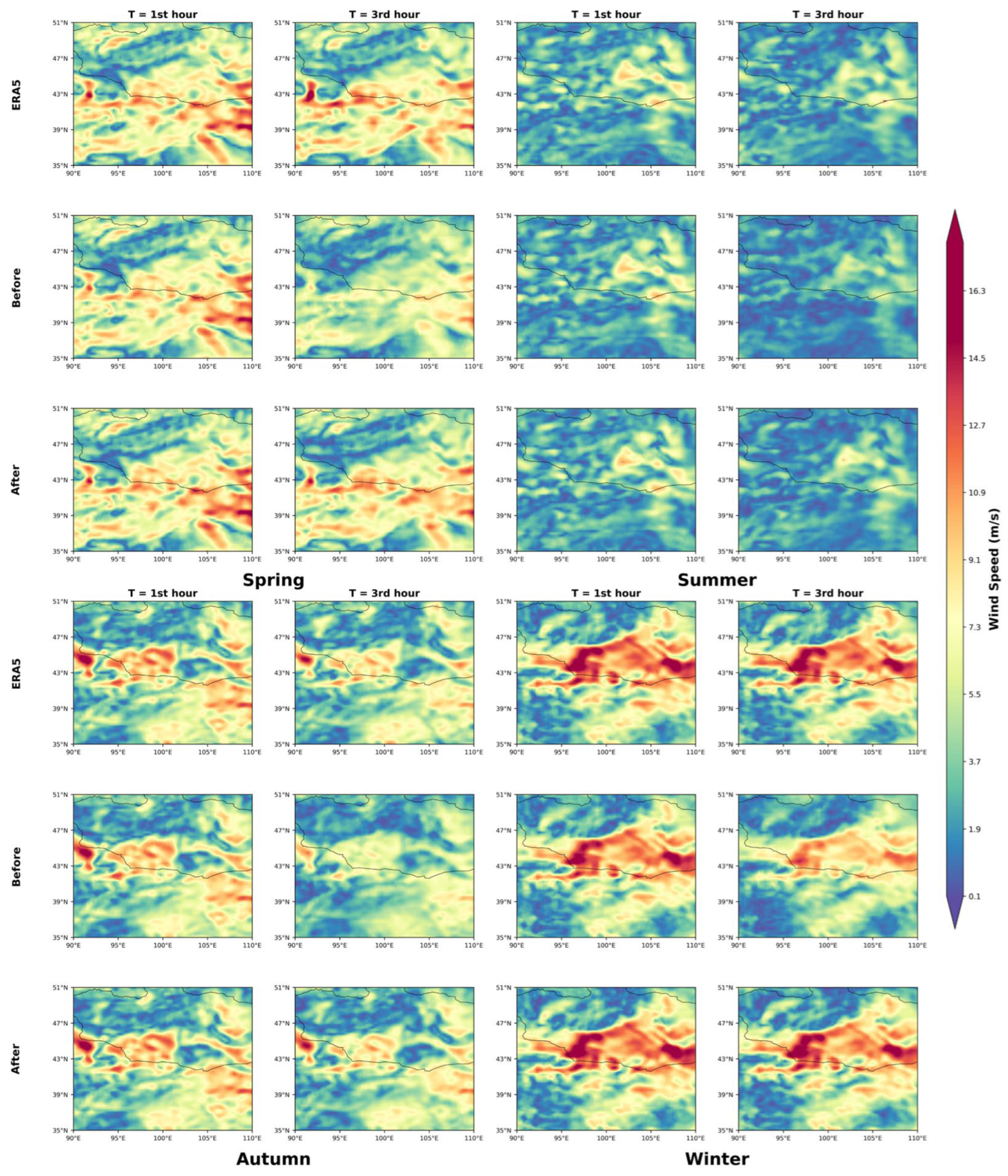
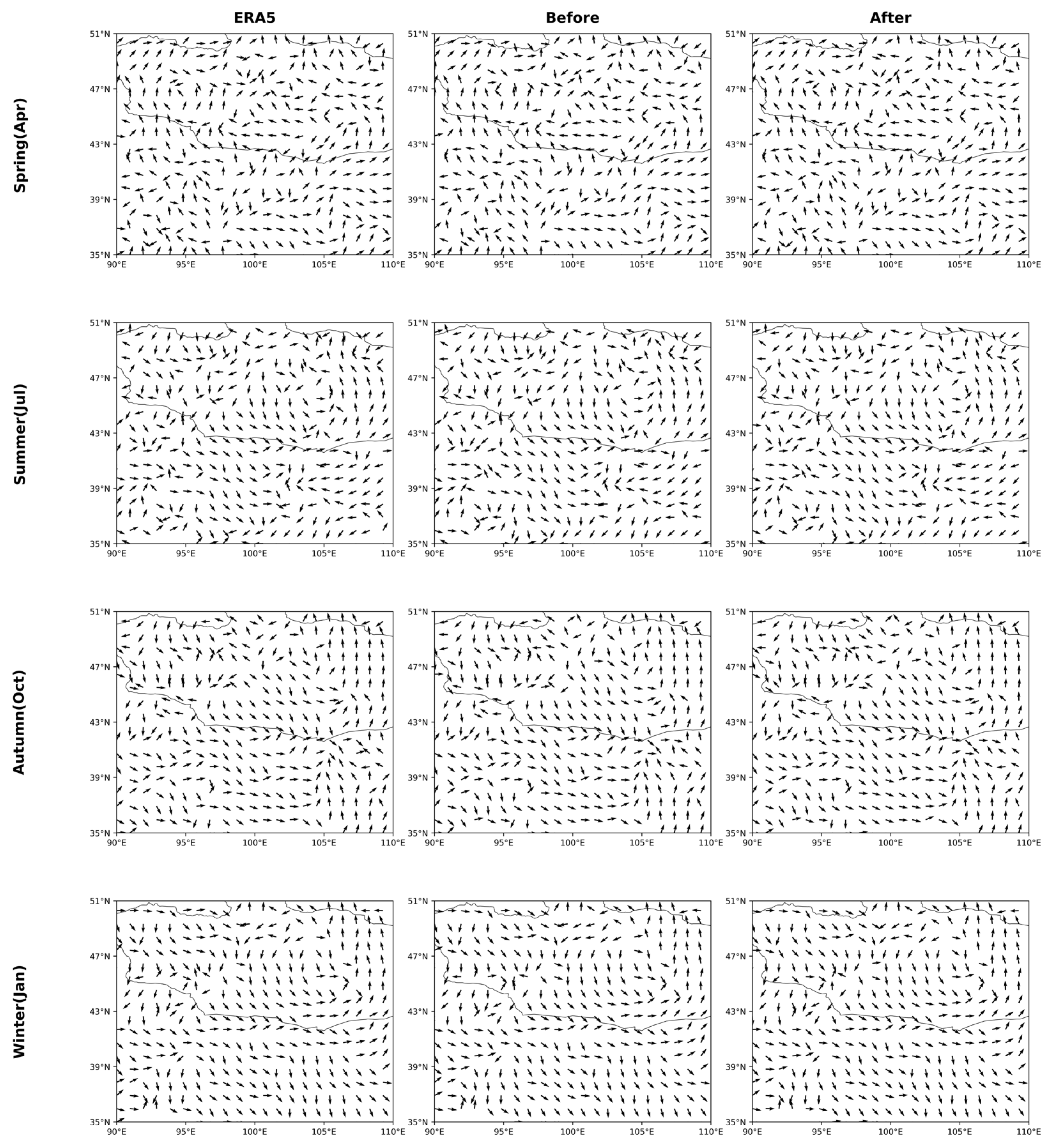
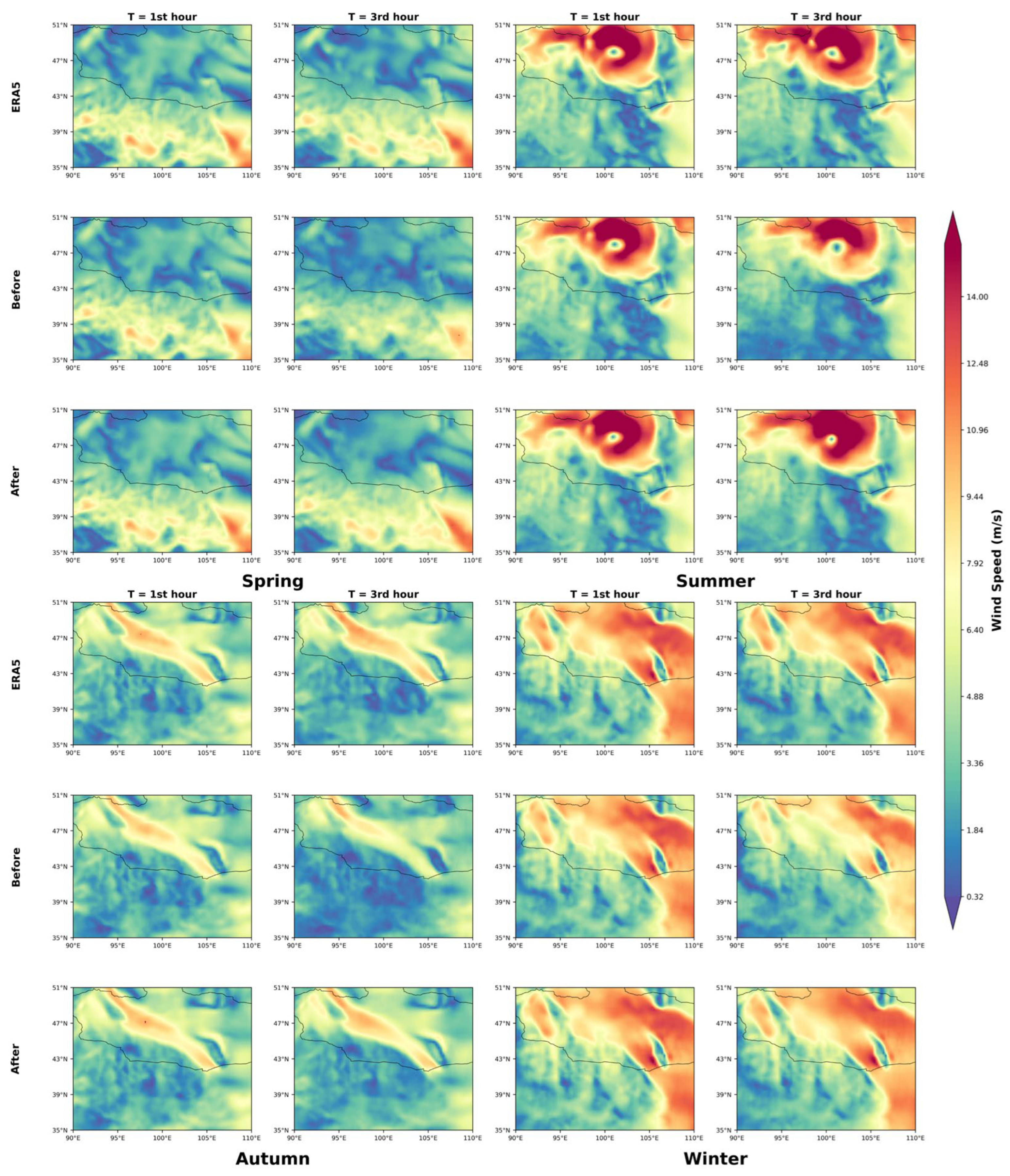
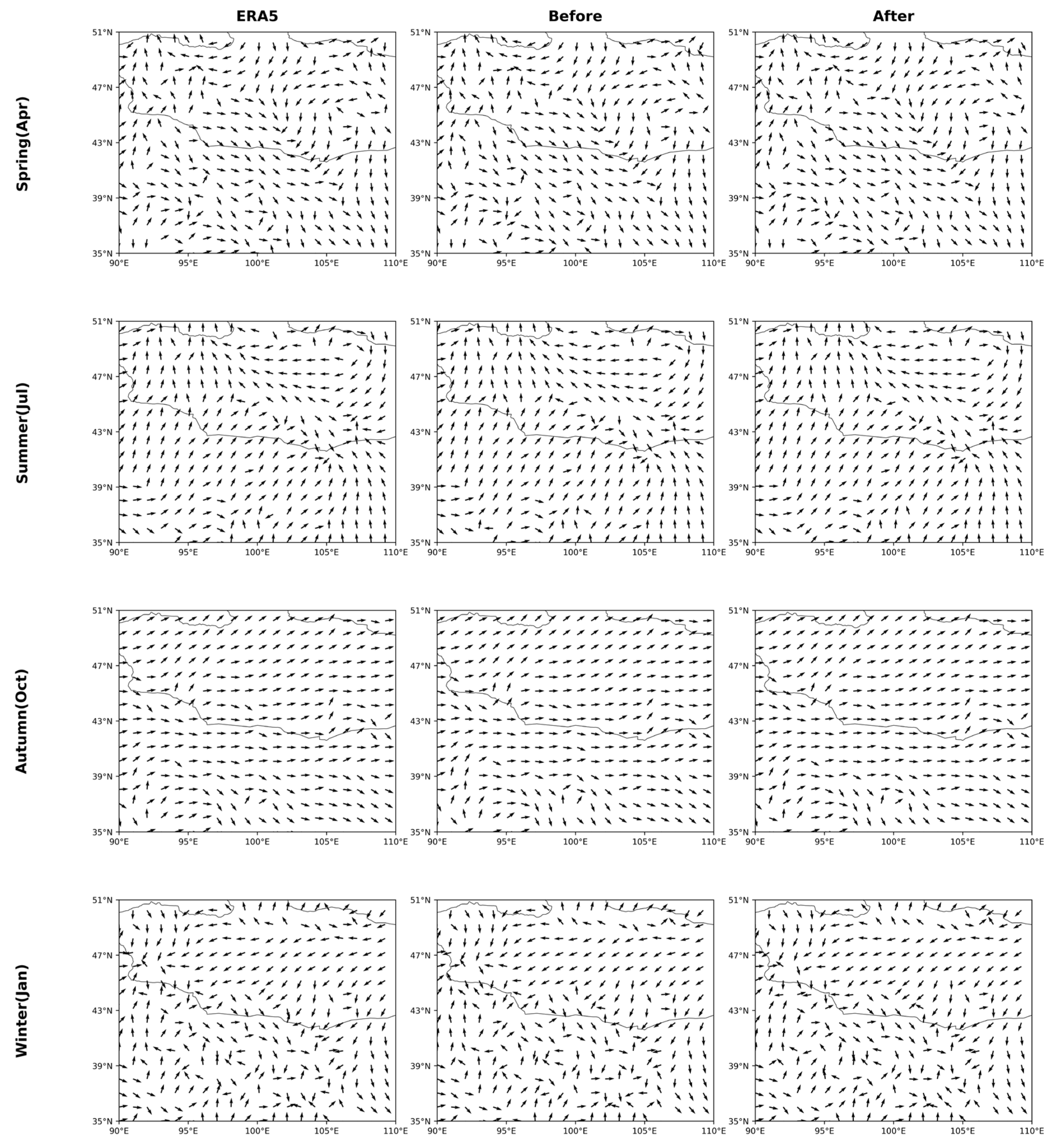
Both sets of visualizations consistently show that, after fine-tuning, AMBHFN produces wind speed and wind direction fields that are more consistent with ERA5 observations, with clear improvements in spatial alignment. Figure 7 and Figure 8 present seasonal wind speed and wind direction predictions, respectively, in which ERA5 data are used as the ground truth, “Before” denotes the results before fine-tuning, and “After” denotes the results after fine-tuning.

As shown in Figure 7, wind speed predictions are systematically improved after fine-tuning. In spring, underestimated high-value centers are restored. In summer, low-wind regions are more accurately captured. In autumn and winter, weakened medium-to-high wind bands are better recovered. Moreover, from T = 1 h to T = 3 h, spatial structures remain more stable after fine-tuning, with reduced blurring and deformation compared with the results before fine-tuning.

As shown in Figure 8, wind direction predictions after fine-tuning are more consistent with ERA5 observations, with reduced local deviations. Overall, both wind speed magnitude reconstruction and the spatial consistency of wind direction are improved through fine-tuning.

Taken together, Figure 9 and Figure 10 show consistent spatial improvements after fine-tuning across the southeastern coastal region of China and Southeast Asia.

For wind speed, ERA5 exhibits a clear banded zone of moderate-to-high wind speeds and localized high-value cores across seasons. Before fine-tuning, these structures are weakened or spatially contracted, with underestimated intensity and blurred gradients. After fine-tuning, both the magnitude and spatial extent are better restored, with improved alignment of banded structures in spring, recovered high-value cores in summer, enhanced gradients in autumn, and sharper strong-wind bands in winter.

For wind direction, noticeable fine-scale deviations are observed before fine-tuning, while after fine-tuning, the flow structures become more consistent with ERA5 observations, and local directional coherence is improved.

Overall, the reconstruction of spatial wind speed structures and the consistency of wind direction fields are significantly improved through fine-tuning, while stable patterns are maintained at T = 3 h, demonstrating strong adaptability to regions with complex monsoon circulation and land–sea interactions.

3.4. Analysis of Model Efficiency

Inference speed and resource consumption are key metrics for evaluating deployment potential.

Table 10. Comparison of computational cost, inference efficiency, and resource consumption among different wind vector prediction models.

Models	GFLOPs	Forward Inference Time [ms/Sample]	Parameter Count [M]	Peak GPU Memory [MB]
TCN	423	14	0.72	547
ConvLSTM	111	28	3.6	588
TropiCycloneNet	126	34	8.4	642
E3DLSTM	123	195	14.8	934
MMVP	375	71	31.8	766
STDGN	58	56	6.9	604
MFWPN	124	18	19.5	321
AMBHFN	128	22	41.1	465

compares different models in terms of computational cost (GFLOPs), average per-sample forward inference time measured with a batch size of 4, parameter count, and peak GPU memory consumption, thereby reflecting the trade-off among accuracy, efficiency, and deployment cost. All efficiency metrics for the compared models are measured using the same NVIDIA GeForce RTX 4090D GPU (NVIDIA Corporation, Santa Clara, CA, USA) and an inference batch size of 4. The input meteorological tensor has a size of (4, 24, 4, 64, 80), corresponding to a 24 h input sequence with four meteorological channels, and the terrain input has a size of (64, 80). The output sequence length is 24 h. The reported forward inference time refers to the average per-sample forward-pass time and excludes data loading, preprocessing, and disk I/O. GPU memory consumption denotes the peak GPU memory during inference.

Clear and pronounced differences are observed among the models. It should be noted that GFLOPs and latency are not strictly proportional, because inference time is also affected by operator type, parallelization efficiency, memory access, and recurrent or graph-based sequential dependencies. For example, TCN has high GFLOPs but benefits from highly parallel convolutional operations, while ConvLSTM and E3DLSTM require recurrent spatiotemporal state updates, leading to longer latency despite their lower GFLOPs. MMVP has relatively high computational cost and a large parameter count, while E3DLSTM has moderate GFLOPs but exhibits the highest inference time and high GPU memory consumption. STDGN and ConvLSTM have lower computational cost but provide only limited practical speed advantages because of graph-based or recurrent operations.

In contrast, AMBHFN achieves a balanced efficiency profile, with 128 GFLOPs, 41.1 M parameters, 465 MB peak GPU memory consumption, and a per-sample forward inference time of 22 ms. Although AMBHFN has more parameters than MFWPN, its GPU memory consumption remains moderate and its latency is close to that of lightweight models such as ConvLSTM. Compared with E3DLSTM and MMVP, AMBHFN achieves lower inference latency with moderate computational and memory requirements.

Overall, AMBHFN achieves a favorable efficiency trade-off, combining fast forward inference with reasonable computational cost, moderate GPU memory consumption, and practical deployment potential.

3.5. Ablation Experiment

To validate the contributions of the MFWVP pathway, 3D UFC pathway, iTMASGC pathway, and the multi-branch fusion mechanism, a set of ablation studies is conducted on AMBHFN. Following a strict single-variable control strategy, each core branch is removed individually from the full model while keeping all other settings unchanged, including the remaining architectural settings, training hyperparameters, the dataset, and evaluation metrics. Experiments are performed on the ERA5 test set in Northeast China.

Table 11. Ablation study of AMBHFN key components using RMSE, MAE and ACC for wind speed prediction.

Metrics	Models	0 h	1 h	2 h	3 h	4–6 h	7–12 h	13–23 h
RMSE	AMBHFN	0.33	0.57	0.74	0.86	1.06	1.42	1.94
	w/o MFWVP	0.58	0.71	0.83	0.93	1.10	1.43	1.96
	w/o 3D UFC	0.40	0.64	0.80	0.92	1.09	1.44	1.95
	w/o iTMASGC	0.34	0.58	0.75	0.86	1.08	1.43	2.01
MAE	AMBHFN	0.25	0.43	0.56	0.65	0.80	1.06	1.49
	w/o MFWVP	0.44	0.54	0.63	0.71	0.83	1.08	1.52
	w/o 3D UFC	0.30	0.49	0.61	0.70	0.83	1.09	1.50
	w/o iTMASGC	0.26	0.44	0.57	0.67	0.82	1.08	1.55
ACC	AMBHFN	0.99	0.97	0.95	0.93	0.90	0.81	0.64
	w/o MFWVP	0.97	0.95	0.94	0.92	0.88	0.79	0.61
	w/o 3D UFC	0.98	0.96	0.94	0.92	0.89	0.80	0.63
	w/o iTMASGC	0.98	0.97	0.94	0.92	0.89	0.80	0.60

and

Table 12. Ablation study of AMBHFN key components using WDFA for wind direction prediction.

Models		0 h (%)			3 h (%)			6 h (%)			12 h (%)
	α = 90	α = 45	α = 22.5	α = 90	α = 45	α = 22.5	α = 90	α = 45	α = 22.5	α = 90	α = 45	α = 22.5
AMBHFN	99.82	99.36	97.72	98.50	94.95	85.18	97.33	91.58	78.06	93.16	81.90	63.23
w/o MFWVP	99.32	97.65	92.56	98.17	94.07	83.18	96.99	90.67	76.46	92.77	81.16	62.03
w/o 3D UFC	99.74	99.07	96.76	98.34	94.38	83.48	97.21	91.03	76.40	93.14	81.42	61.82
w/o iTMASGC	99.80	99.33	97.60	98.44	94.78	84.79	97.25	90.88	77.48	93.09	81.75	62.92

report the performance changes after removing each component, thereby enabling both the individual contributions and the overall synergistic effects of the full architecture to be analyzed.

In the ablation study of the MFWVP pathway, this branch is removed while the 3D UFC, iTMASGC, and fusion mechanism are retained. Results show a clear performance drop across all forecast horizons. RMSE and MAE increase noticeably, ACC decreases consistently, and the degradation is most pronounced at 0 h, where RMSE increases from 0.33 m/s to 0.58 m/s and MAE rises from 0.25 m/s to 0.44 m/s. WDFA also decreases, indicating a weakened ability to reconstruct wind direction. These results indicate that MFWVP is a key contributor to prediction accuracy.

In the ablation study of the 3D UFC pathway, removing this branch leads to increased RMSE and MAE, reduced ACC, and a slight overall performance degradation across forecast horizons. At 0 h, RMSE increases to 0.40 m/s and MAE rises to 0.30 m/s. WDFA decreases across all forecast lead times, indicating a weakened capability to capture global spatial structures and maintain long-term spatial consistency.

In the ablation study of the iTMASGC pathway, removing this branch causes a noticeable overall degradation. Wind speed errors increase, with RMSE reaching 2.01 m/s and MAE reaching 1.55 m/s over the 13–23 h forecast range, while ACC drops to 0.60. Together with the slight decline in WDFA, these results indicate weaker long-range temporal modeling and reduced forecasting robustness.

The ablation results show that the contributions of the three core pathways can be ranked in descending order as MFWVP, 3D UFC, and iTMASGC in this experimental setting. The MFWVP pathway is the most influential component, as it captures rapid wind-field variations and localized abrupt changes, making the largest contribution to short-term forecasting over 0–6 h. The 3D UFC pathway mainly provides global spatiotemporal structure modeling, ensuring structural consistency across all forecast lead times. The iTMASGC pathway mainly enhances temporal robustness and reduces error accumulation, playing a key role in longer-term forecasting over 12–23 h. Through the prediction-level adaptive multi-branch fusion mechanism, these three pathways complement each other and jointly support stable and high-precision wind forecasting across all horizons.

4. Discussion

In AMBHFN, the wind vector prediction task is explicitly decomposed into local dynamic modeling, global structural modeling, and temporal robustness modeling. These objectives are assigned to heterogeneous prediction branches and coordinated through adaptive prediction-level fusion. Based on the quantitative results presented in Section 3, the architectural and modeling factors associated with the observed performance differences are interpreted in this section.

(1) Task-Oriented Functional Decomposition: The overall comparison and transfer experiments support the effectiveness of task-oriented prediction decomposition. By assigning the prediction objectives of local dynamic modeling, global structural modeling, and temporal robustness modeling to dedicated branches, AMBHFN reduces interference among heterogeneous wind-field characteristics and maintains balanced performance across different forecast horizons and regions.

(2) Heterogeneous Collaborative Architecture for Wind Field Forecasting: The ablation and visualization results confirm the complementary roles of the three prediction branches. MFWVP focuses on local wind-field variations, 3D UFC preserves global spatiotemporal structures, and iTMASGC enhances temporal stability. Their parallel organization enables specialized modeling while allowing different prediction capabilities to complement one another.

(3) Prediction-Level Adaptive Collaboration Mechanism: The overall prediction results and the learned path weights support the effectiveness of AMBPC. Through the combination of identity mapping, global dependency modeling, and local spatiotemporal interaction, the outputs of MFWVP, 3D UFC, and iTMASGC are adaptively coordinated by AMBPC. This prediction-level collaboration preserves branch-specific information while integrating complementary prediction patterns.

(4) Multi-Agent Graph-Enhanced Temporal Robustness Modeling: The multi-horizon stability analysis and iTMASGC ablation results support the effectiveness of graph-enhanced multi-agent temporal modeling. Diverse temporal patterns are independently captured by the temporal agents, while information exchange is enabled through graph-based interaction, thereby improving temporal consistency. This design helps reduce error accumulation and maintain greater stability in long-horizon prediction.

Overall, the results demonstrate that task-oriented prediction decomposition, heterogeneous branch collaboration, adaptive prediction-level coordination, and graph-enhanced temporal modeling jointly improve wind vector prediction performance.

5. Conclusions

AMBHFN is proposed for wind vector prediction based on task-oriented functional decomposition and heterogeneous branch collaboration. The forecasting task is decomposed into local dynamic modeling, global structural modeling, and temporal robustness modeling, and the corresponding branches are coordinated through AMBPC. Through the integration of multi-source meteorological variables, terrain information, 3D UFC, iTMASGC, and adaptive prediction collaboration, AMBHFN jointly preserves local details, global structures, and temporal consistency.

Experiments show that AMBHFN achieves lower RMSE and MAE than eight retrained baselines over the 0–23 h forecast horizon, reducing average errors by over 12%. The first-hour RMSE and MAE are 0.33 m/s and 0.25 m/s, respectively, while WDFA under the strict 22.5° threshold reaches 97.72% at 0 h and 78.06% at 6 h. Paired t-tests and Wilcoxon signed-rank tests against MFWPN confirm statistically significant improvements in weighted RMSE, MAE, ACC, and WDFA under the 90°, 45°, and 22.5° thresholds. In cross-regional transfer experiments, fine-tuning reduces RMSE over 13–23 h to 1.54 and 1.96 and increases the 12 h WDFA under the 22.5° threshold to 74.08% and 63.06% in the two target regions, demonstrating adaptability to heterogeneous climatic and geographic conditions.

Ablation studies confirm the complementary roles of the heterogeneous branches, while visualization and stability analyses demonstrate consistent spatial reconstruction and controlled error growth. AMBHFN has a computational cost of 128 GFLOPs, contains 41.1 M parameters, requires 465 MB of peak GPU memory, and requires 22 ms per sample for forward inference, thereby achieving a favorable balance between predictive accuracy and deployment cost.

Future work will develop and evaluate the model using longer multi-year datasets and more diverse scenarios, including rolling-year evaluation, wind prediction at the 10 m station height, and multi-height wind vector prediction, to enhance generalization and practical applicability.

References

1. Resifi, S.; Al Aawar, E.; Dasari, H.P.; Jebari, H.; Hoteit, I. A novel deep learning approach for regional high-resolution spatio-temporal wind speed forecasting for energy applications. Energy 2025, 328, 136356. [Google Scholar] [CrossRef] [Scilit]
2. Veers, P.; Dykes, K.; Basu, S.; Bianchini, A.; Clifton, A.; Green, P.; Holttinen, H.; Kitzing, L.; Kosovic, B.; Lundquist, J.K.; et al. Grand Challenges: Wind energy research needs for a global energy transition. Wind Energy Sci. 2022, 7, 2491–2496. [Google Scholar] [CrossRef] [Scilit]
3. Xie, L.; Gu, Y.; Zhu, X.; Genton, M.G. Power system economic dispatch with spatio-temporal wind forecasts. In Proceedings of the 2011 EnergyTech; IEEE: New York, NY, USA, 2011; pp. 1–6. [Google Scholar]
4. Neumann, C.J.; Lawrence, M.B. An operational experiment in the statistical-dynamical prediction of tropical cyclone motion. Mon. Weather Rev. 1975, 103, 665–673. [Google Scholar] [CrossRef] [Scilit]
5. Chen, X.; Zhang, F. Development of a convection-permitting air-sea-coupled ensemble data assimilation system for tropical cyclone prediction. J. Adv. Model. Earth Syst. 2019, 11, 3474–3496. [Google Scholar] [CrossRef] [Scilit]
6. Tang, X.Y.; Zhao, S.; Fan, B.; Peinke, J.; Stoevesandt, B. Micro-scale wind resource assessment in complex terrain based on CFD coupled measurement from multiple masts. Appl. Energy 2019, 238, 806–815. [Google Scholar] [CrossRef] [Scilit]
7. Hill, D.C.; McMillan, D.; Bell, K.R.W.; Infield, D. Application of auto-regressive models to UK wind speed data for power system impact studies. IEEE Trans. Sustain. Energy 2011, 3, 134–141. [Google Scholar]
8. Rajagopalan, S.; Santoso, S. Wind power forecasting and error analysis using the autoregressive moving average modeling. In Proceedings of the 2009 IEEE Power & Energy Society General Meeting; IEEE: New York, NY, USA, 2009. [Google Scholar]
9. Erdem, E.; Shi, J. ARMA based approaches for forecasting the tuple of wind speed and direction. Appl. Energy 2011, 88, 1405–1414. [Google Scholar] [CrossRef] [Scilit]
10. Singh, S.N.; Mohapatra, A. Repeated wavelet transform based ARIMA model for very short-term wind speed forecasting. Renew. Energy 2019, 136, 758–768. [Google Scholar] [CrossRef] [Scilit]
11. Shukur, O.B.; Lee, M.H. Daily wind speed forecasting through hybrid KF-ANN model based on ARIMA. Renew. Energy 2015, 76, 637–647. [Google Scholar] [CrossRef] [Scilit]
12. Tian, Z.; Li, H.; Li, F. A combination forecasting model of wind speed based on decomposition. Energy Rep. 2021, 7, 1217–1233. [Google Scholar] [CrossRef] [Scilit]
13. Liu, Z.; Jiang, P.; Zhang, L.; Niu, X. A combined forecasting model for time series: Application to short-term wind speed forecasting. Appl. Energy 2020, 259, 114137. [Google Scholar] [CrossRef] [Scilit]
14. Zhou, H.; Wang, Z. A multiple-model based adaptive control algorithm for very-short term wind power forecasting. In Proceedings of the 2016 International Conference on Power System Technology (POWERCON); IEEE: New York, NY, USA, 2016; pp. 1–6. [Google Scholar]
15. Hoolohan, V.; Tomlin, A.S.; Cockerill, T. Improved near surface wind speed predictions using Gaussian process regression combined with numerical weather predictions and observed meteorological data. Renew. Energy 2018, 126, 1043–1054. [Google Scholar] [CrossRef] [Scilit]
16. Zhang, Z.; Lin, L.; Gao, S.; Wang, J.; Zhao, H. Wind speed prediction in China with fully-convolutional deep neural network. Renew. Sustain. Energy Rev. 2024, 201, 114623. [Google Scholar] [CrossRef] [Scilit]
17. Hochreiter, S.; Schmidhuber, J. Long short-term memory. Neural Comput. 1997, 9, 1735–1780. [Google Scholar] [CrossRef] [Scilit] [PubMed]
18. Chung, J.; Gulcehre, C.; Cho, K.H.; Bengio, Y. Empirical evaluation of gated recurrent neural networks on sequence modeling. arXiv 2014, arXiv:1412.3555. [Google Scholar]
19. Zhang, H.; Wang, J.; Qian, Y.; Li, Q. Point and interval wind speed forecasting of multivariate time series based on dual-layer LSTM. Energy 2024, 294, 130875. [Google Scholar] [CrossRef] [Scilit]
20. Jaseena, K.U.; Kovoor, B.C. Decomposition-based hybrid wind speed forecasting model using deep bidirectional LSTM networks. Energy Convers. Manag. 2021, 234, 113944. [Google Scholar] [CrossRef] [Scilit]
21. Li, C.; Tang, G.; Xue, X.; Saeed, A.; Hu, X. Short-term wind speed interval prediction based on ensemble GRU model. IEEE Trans. Sustain. Energy 2019, 11, 1370–1380. [Google Scholar] [CrossRef] [Scilit]
22. Shi, X.; Chen, Z.; Wang, H.; Yeung, D.Y.; Wong, W.K.; Woo, W.C. Convolutional LSTM network: A machine learning approach for precipitation nowcasting. In Advances in Neural Information Processing Systems 28; Neural Information Processing Systems Foundation, Inc.: South Lake Tahoe, NV, USA, 2015. [Google Scholar]
23. Wang, Y.; Jiang, L.; Yang, M.H.; Li, L.J.; Long, M.; Li, F.-F. Eidetic 3D LSTM: A model for video prediction and beyond. In Proceedings of the International Conference on Learning Representations, Vancouver, BC, Canada, 30 April–3 May 2018. [Google Scholar]
24. Chen, Y.; Zhang, S.; Zhang, W.; Peng, J.; Cai, Y. Multifactor spatio-temporal correlation model based on a combination of convolutional neural network and long short-term memory neural network for wind speed forecasting. Energy Convers. Manag. 2019, 185, 783–799. [Google Scholar] [CrossRef] [Scilit]
25. Khodayar, M.; Wang, J. Spatio-temporal graph deep neural network for short-term wind speed forecasting. IEEE Trans. Sustain. Energy 2018, 10, 670–681. [Google Scholar]
26. Lin, S.; Wang, S.; Xu, X.; Li, R.; Shi, P. GAOformer: An adaptive spatiotemporal feature fusion transformer utilizing GAT and optimizable graph matrixes for offshore wind speed prediction. Energy 2024, 292, 130404. [Google Scholar] [CrossRef] [Scilit]
27. Gao, S.; Meng, G.; Lin, L.; Zhang, Z.; Wang, J.; Zhao, H. Spatiotemporal MultiWaveNet for efficiently generating environmental spatiotemporal series. IEEE Trans. Geosci. Remote Sens. 2024, 62, 4107417. [Google Scholar] [CrossRef] [Scilit]
28. Gao, Z.; Shi, X.; Wang, H.; Zhu, Y.; Wang, Y.B.; Li, M.; Yeung, D.Y. Earthformer: Exploring space-time transformers for earth system forecasting. Adv. Neural Inf. Process. Syst. 2022, 35, 25390–25403. [Google Scholar] [CrossRef] [Scilit]
29. Chen, L.; Zhong, X.; Zhang, F.; Cheng, Y.; Xu, Y.; Qi, Y.; Li, H. FuXi: A cascade machine learning forecasting system for 15-day global weather forecast. npj Clim. Atmos. Sci. 2023, 6, 190. [Google Scholar] [CrossRef] [Scilit]
30. Li, Q.; Wang, G.; Wu, X.; Gao, Z.; Dan, B. Arctic short-term wind speed forecasting based on CNN-LSTM model with CEEMDAN. Energy 2024, 299, 131448. [Google Scholar] [CrossRef] [Scilit]
31. Altan, A.; Karasu, S.; Zio, E. A new hybrid model for wind speed forecasting combining long short-term memory neural network, decomposition methods and grey wolf optimizer. Appl. Soft Comput. 2021, 100, 106996. [Google Scholar] [CrossRef] [Scilit]
32. Chen, J.; Zeng, G.Q.; Zhou, W.; Du, W.; Lu, K.D. Wind speed forecasting using nonlinear-learning ensemble of deep learning time series prediction and extremal optimization. Energy Convers. Manag. 2018, 165, 681–695. [Google Scholar] [CrossRef] [Scilit]
33. Wang, J.; Che, J.; Li, Z.; Gao, J.; Zhang, L. Hybrid wind speed optimization forecasting system based on linear and nonlinear deep neural network structure and data preprocessing fusion. Future Gener. Comput. Syst. 2025, 164, 107565. [Google Scholar] [CrossRef] [Scilit]
34. Wu, T.; Ling, Q. STELLM: Spatio-temporal enhanced pre-trained large language model for wind speed forecasting. Appl. Energy 2024, 375, 124034. [Google Scholar] [CrossRef] [Scilit]
35. He, J.; Hu, Z.; Wang, S.; Mujeeb, A.; Yang, P. Windformer: A novel 4D high-resolution system for multi-step wind speed vector forecasting based on temporal shifted window multi-head self-attention. Energy 2024, 310, 133206. [Google Scholar] [CrossRef] [Scilit]
36. Huang, G.; Li, H.; Mo, X.; Jian, X. A novel dynamic spatio-temporal graph convolutional network with multi-scale transformer for high-resolution wind vector forecasting. Energy Convers. Manag. X 2026, 30, 101684. [Google Scholar] [CrossRef] [Scilit]
37. Huang, G.; Li, H.; Mo, X. A novel point-interval prediction model for wind speed based on hybrid deep learning and RIME optimization algorithms. Energy Rep. 2025, 14, 3977–3992. [Google Scholar] [CrossRef] [Scilit]
38. Wang, J.; Mo, W.; Wu, Y.; Xu, X.; Li, Y.; Ye, J.; Lai, X. Combined channel attention and spatial attention module network for chinese herbal slices automated recognition. Front. Neurosci. 2022, 16, 920820. [Google Scholar] [CrossRef] [Scilit] [PubMed]
39. Zhang, Z.; Lin, L.; Gao, S.; Wang, J.; Zhao, H.; Yu, H. A machine learning model for hub-height short-term wind speed prediction. Nat. Commun. 2025, 16, 3195. [Google Scholar] [CrossRef] [Scilit] [PubMed]
40. Li, P.; Yin, L.; Liu, S. Mix-ln: Unleashing the power of deeper layers by combining pre-ln and post-ln. arXiv 2024, arXiv:2412.13795. [Google Scholar]
41. Huang, C.; Mu, P.; Zhang, J.; Chan, S.; Zhang, S.; Yan, H.; Chen, S.; Bai, C. Benchmark dataset and deep learning method for global tropical cyclone forecasting. Nat. Commun. 2025, 16, 5923. [Google Scholar] [CrossRef] [Scilit] [PubMed]
42. Liu, Y.; Hu, T.; Zhang, H.; Wu, H.; Wang, S.; Ma, L.; Long, M. itransformer: Inverted transformers are effective for time series forecasting. arXiv 2023, arXiv:2310.06625. [Google Scholar]
43. Ding, S.; Du, W.; Ding, L.; Guo, L.; Zhang, J. Learning efficient and robust multi-agent communication via graph information bottleneck. Proc. AAAI Conf. Artif. Intell. 2024, 38, 17346–17353. [Google Scholar] [CrossRef] [Scilit]
44. Bai, S.; Kolter, J.Z.; Koltun, V. An empirical evaluation of generic convolutional and recurrent networks for sequence modeling. arXiv 2018, arXiv:1803.01271. [Google Scholar]
45. Zhong, Y.; Liang, L.; Zharkov, I.; Neumann, U. Mmvp: Motion-matrix-based video prediction. In Proceedings of the IEEE/CVF International Conference on Computer Vision; IEEE: New York, NY, USA, 2023; pp. 4273–4283. [Google Scholar]
46. Tan, C.; Gao, Z.; Wu, L.; Xu, Y.; Xia, J.; Li, S.; Li, S.Z. Temporal attention unit: Towards efficient spatiotemporal predictive learning. In Proceedings of the IEEE/CVF Conference on Computer Vision and Pattern Recognition; IEEE: New York, NY, USA, 2023; pp. 18770–18782. [Google Scholar]
47. Wang, J.; Lin, L.; Gao, S.; Zhang, Z. Deep generation network for multivariate spatio-temporal data based on separated attention. Inf. Sci. 2023, 633, 85–103. [Google Scholar] [CrossRef] [Scilit]
Figure 1. Digital elevation model of the main experimental area and transfer experimental area.
Energies 19 03406 g001
Figure 2. Overall architecture of the AMBHFN.
Energies 19 03406 g002
Figure 3. Learned Fusion Weights of the Three Collaboration Paths in AMBPC.
Energies 19 03406 g003
Figure 4. Visualization results of wind speed prediction (WSP) in Northeast China.
Energies 19 03406 g004
Figure 5. Visualization of wind direction prediction results in Northeast China.
Energies 19 03406 g005
Figure 6. Comparison of RMSE, MAE, ACC and WDFA across different models: (a) wind speed RMSE; (b) wind speed MAE; (c) anomaly correlation coefficient (ACC); and (d) wind direction forecast accuracy (WDFA) at α = 22 . 5 .
Energies 19 03406 g006
Figure 7. Wind speed prediction visualization for northern China and the Mongolian Plateau.
Energies 19 03406 g007
Figure 8. Wind direction prediction visualization for northern China and the Mongolian Plateau.
Energies 19 03406 g008
Figure 9. Wind speed prediction visualization for southeastern coastal China and Southeast Asia.
Energies 19 03406 g009
Figure 10. Wind direction prediction visualization for southeastern coastal China and Southeast Asia.
Energies 19 03406 g010