A Unified ANN-Based Approach for Fault Classification, Location and CCT-Based Stability Assessment in HVAC Transmission Systems

Abstract

Accurate and fast fault detection is essential to ensure the stability and reliability of High Voltage AC (HVAC) transmission systems. Conventional protection methods, including impedance-based and traveling wave techniques, may exhibit reduced performance under noisy operating conditions, system uncertainties, and complex fault scenarios while often requiring separate approaches for fault classification, location detection, and stability assessment. This paper proposes a unified Artificial Neural Network (ANN) based framework for simultaneous fault classification, location detection, and stability assessment using Critical Clearing Time (CCT) within a single HVAC transmission line model. A detailed MATLAB Simulink model is developed to generate a structured dataset comprising twelve fault scenarios, including single-line, double-line, three-phase, and ground faults at different locations along the transmission line. Three-phase voltages and currents, along with zero-sequence components, are used as input features. The ANN model is trained using the Levenberg–Marquardt (LM) optimization algorithm, which was comparatively evaluated against Bayesian Regularization (BR) and Scaled Conjugate Gradient (SCG) and demonstrated faster convergence, lower prediction error, and higher regression accuracy. To further evaluate the robustness of the proposed framework under high-impedance fault conditions, supplementary simulations were performed using fault resistance values of 10 Ω and 50 Ω in addition to the baseline 0.01 Ω case. The resulting datasets were combined to form an expanded training and evaluation dataset, enabling comprehensive validation of the proposed LM-trained ANN under varying fault resistance conditions. Using the baseline dataset, the proposed framework achieved a high regression coefficient (R = 0.9882) and low mean squared error (MSE = 0.1386), demonstrating accurate fault classification and precise per-kilometer fault location estimation. Furthermore, the integration of fault inception time and duration enables direct computation of CCT, allowing the model to distinguish between stability-critical and non-critical fault conditions. The results confirm that the proposed framework provides a comprehensive and efficient solution for real-time fault analysis by combining classification, localization, temporal analysis, and stability-aware decision support within a single model.

1. Introduction

Growing industrial development has significantly increased energy demand, driving the need for efficient high voltage power transmission systems. Advances in power electronics have enhanced the capability of high voltage transmission lines to transfer large amounts of power over long distances. Nowadays, different High Voltage DC (HVDC) transmission technologies based on advanced converter configurations have been developed to address challenges associated with long-distance and offshore power transmission. HVAC transmission remains widely used for short to medium distances due to its operational simplicity, ease of voltage transformation, and suitability for multi-generator interconnections [1]. HVDC transmission offers lower losses, eliminates reactive power issues, and enables interconnection of asynchronous grids, making it more suitable for long-distance, submarine, and bulk power transfer applications. HVAC is generally preferred for regional transmission networks, while HVDC is adopted for specialized long-distance and high-capacity transmission requirements [2]. The electrification and digitalization of mobility systems, including innovative tramway lines, electric bus depots, vehicle-to-grid applications, real-driving EV modeling, and energy-demand models for battery e-buses, further increase the interaction between transport loads and electrical networks. Such applications reinforce the need for resilient power infrastructures capable of maintaining secure operation under faults and dynamic loading conditions [3,4,5,6]. Reliability is reduced by conventional protection methods based on voltage derivatives and traveling wave analysis, as they are highly sensitive to fault resistance, particularly in high-impedance fault conditions [7]. When DC voltage drops are used exclusively, fault detection between internal and external zones becomes unstable. These drawbacks highlight the necessity for more advanced and reliable protection methods for HVDC systems to allow more precise and rapid detection of faults. Due to its advantages in high-capacity energy transfer, asynchronous grid connections, and long-distance power transmission, which are crucial to modern large-scale power systems, reliable HVDC protection is crucial as AC/DC hybrid networks become more integrated [8]. Particularly in industrial applications, early fault detection is essential for maintaining power system stability and minimizing outage duration. Transmission line faults have a more significant negative impact on system performance than faults in lower voltage networks. Hence, significant research has been conducted on their rapid fault detection and accurate localization. Fault location algorithms integrated into protection systems are often used to identify the fault position, as physical inspection of transmission lines is time-consuming. Transmission line faults can be either permanent, requiring safe isolation and maintenance, or transient, self-clearing without causing permanent damage [9].

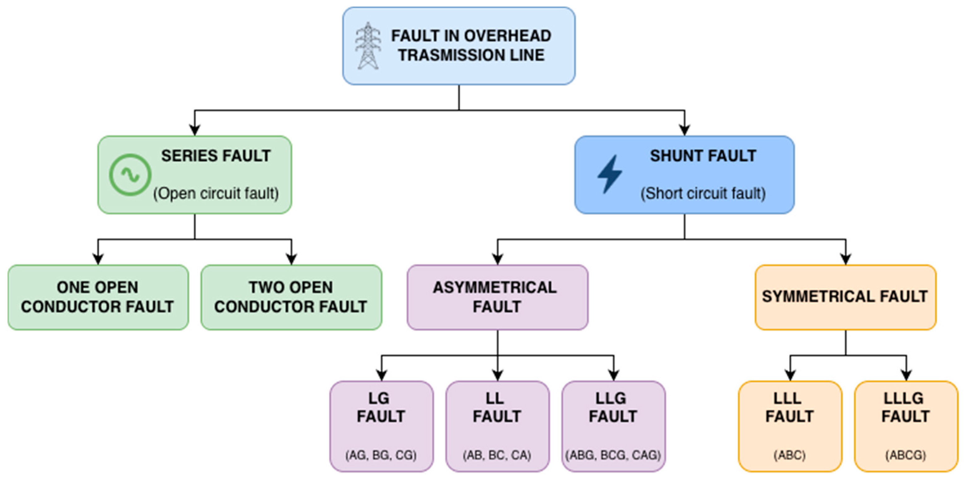
Overhead transmission line faults, which are caused by a number of conditions such as bad weather, human activity, exposure to smoke or fire, and equipment failures, have a significant effect on the reliability and continuity of electrical networks. When electrical features such as voltage, current, or phase angle exceed permissible limits, it is referred to as a fault. Overhead transmission lines are more susceptible to faults than underground cables due to their constant exposure to environmental conditions. In HVAC transmission lines, faults generally appear as open conductor or short circuit conditions that disrupt normal system operation and may lead to service interruptions if not detected and cleared rapidly, as shown in Figure 1. Traditionally, transmission line faults were identified through manual analysis methods. These processes are time-consuming and impractical for long or remote transmission line systems, highlighting the need for automated and intelligent fault detection methods [10].

Reliable fault identification and protection in modern AC transmission lines remain challenging despite significant improvements in HVAC technologies. Traditional methods based on voltage derivatives, traveling waves, or DC voltage drops often perform poorly under high-impedance faults and converter interactions, leading to inaccurate classification and delayed fault isolation. Series of faults, measurement noise, communication delays, and dynamic operating conditions are generally ignored, while short circuit faults remain the main focus of much current research that assumes ideal measurement conditions. There is currently little practical validation of protection solutions for hybrid overhead cable links, offshore systems, and multi-terminal AC networks [11]. These challenges highlight the need for adaptive noise-resilient and computationally efficient fault detection methods capable of accurately identifying and locating diverse fault types in complex AC transmission networks.

To enhance system performance and accurate fault identification, many algorithms have been proposed in recent years, including traditional methods based on fundamental frequency components such as impedance analysis and traveling wave techniques. These traditional methods analyze voltage and current measurements both before and after a disturbance or use reflected wave time delays for fault detection. However, their accuracy often degrades in the presence of noise, system nonlinearities, or high-impedance faults. To address these limitations, this study integrates optimized machine learning methods for precise fault classification and location identification in AC transmission networks using extracted electrical signal features. In comparison to traditional analytical and traveling wave methods, the proposed method significantly improves reliability and detection time by adaptively learning the nonlinear relationships between voltage current patterns and various fault types.

In this research, an LM-trained ANN-based framework is presented for fault classification and location detection in HVAC transmission lines, aiming to overcome these constraints. The model is designed to learn nonlinear fault characteristics from electrical measurements, enabling accurate fault classification and location detection under the considered simulated fault conditions. Unlike conventional ANN-based studies that mainly focus on fault classification or fault location estimation as an independent protection task [12,13,14,15,16,17], the proposed LM-trained multi-output ANN framework simultaneously performs fault classification, fault location estimation, fault timing extraction, and ML-integrated CCT assessment using a unified electrical feature representation within a single prediction model.

The main contributions of the paper are as follows.

• A unified intelligent protection framework is proposed for HVAC transmission systems to simultaneously perform fault classification, fault location estimation, fault timing extraction, and ML-integrated Critical Clearing Time (CCT) assessment using a single LM-trained multi-output ANN and a unified electrical feature representation.
• A comparative evaluation of ANN training algorithms (BR, SCR, and LM) is conducted to determine the most suitable optimization strategy for the proposed multi-output ANN framework. Based on quantitative performance analysis, the LM algorithm is selected due to its superior convergence characteristics, lower prediction error, and higher regression accuracy for unified HVAC fault classification, per km fault location estimation, and ML-integrated CCT assessment.
• Beyond fault types and location detection, the proposed method integrates the Critical Clearing Time (CCT) function to distinguish stability-critical faults from normal conditions, enhancing time-dependent protection decisions and improving overall system resilience. It also extracts fault inception time and fault persistence duration.

This paper presents an LM-trained ANN-based method for fault classification, location estimation, and CCT-based stability assessment in HVAC transmission systems. Section 2 reviews related fault detection methods while Section 3 describes the proposed methodology, including the HVAC model, dataset generation, data processing, ANN structure, and training procedure. Section 4 presents the results, including fault classification, location detection, high-impedance fault evaluation, feature ablation analysis, and CCT-based stability assessment. Finally, Section 5 summarizes the main findings and their significance for intelligent protection applications.

2. Related Work

Fault detection and classification in HVAC transmission systems have been extensively studied using both conventional signal processing techniques and modern data-driven approaches. Existing methods can be broadly categorized into traditional model-based techniques and Artificial Intelligence (AI)-based methods.

2.1. Conventional Fault Detection Methods

Traditional fault detection techniques are primarily based on electrical signal analysis, including impedance-based methods, traveling wave techniques, and frequency domain signal processing. Impedance-based approaches estimate fault location using voltage and current measurements, while traveling wave methods rely on high-frequency transient signals and wave propagation characteristics [18]. Although these methods are effective under ideal operating conditions, their performance is highly sensitive to fault resistance, measurement noise, and parameter uncertainties. In addition, they require precise system modeling and high sampling rates, which limit their applicability in real-time environments [18,19]. Signal processing approaches such as the Discrete Wavelet Transform (DWT) have also been applied for fault detection [20]. However, they often require manual feature extraction and are limited in handling complex nonlinear fault dynamics.

2.2. Machine Learning-Based Methods

To overcome the limitations of conventional techniques, machine learning (ML) approaches have been increasingly adopted for fault classification and detection. Methods such as K-nearest neighbors (KNN) [15], decision trees (DT), logistic regression, and support vector machine (SVM) [12] have been used to classify faults based on extracted electrical features. While these approaches improve classification performance, they are generally limited to specific fault scenarios and often lack generalization capability. In many cases, these models focus solely on classification tasks and do not address fault location detection or temporal analysis. For instance, KNN-based approaches demonstrate basic classification capability but are constrained by system-specific configurations and limited scalability [15,16]. Similarly, hybrid methods combining wavelet transform and optimization algorithms improve accuracy but still lack comprehensive fault analysis, particularly in terms of location estimation and stability assessment [17].

2.3. Deep Learning and Hybrid Approaches

Recent advancements in deep learning have further enhanced fault detection performance in power systems. Convolutional neural networks (CNN), deep neural networks (DNN), and hybrid architectures such as CNN-LSTM have been employed to automatically extract features from raw signals and capture both spatial and temporal fault characteristics [13,14]. Transformer-based models have also been proposed for handling complex nonlinear fault dynamics [21]. Recent review studies have highlighted the rapid expansion of deep learning and data-driven methods in power systems, including fault diagnosis, stability assessment, renewable energy integration, forecasting, intelligent monitoring, and clustering-based analysis, demonstrating the increasing maturity of AI-driven approaches for modern electrical networks [22,23]. Despite their improved accuracy and robustness, these methods typically require large datasets and high computational resources. More importantly, most deep learning-based approaches remain task-specific, focusing primarily on fault classification while neglecting other critical aspects such as fault location, fault duration, and system stability. Only a limited number of studies address fault location detection, and even fewer incorporate stability-related metrics such as CCT into the analysis framework [14]. Kouraichi et al. analyzed CNN, LSTM/GRU, generative models, attention processes, and other DL based fault diagnosis methods for power transmission lines. To highlight the potential of DL models for extracting temporal and high-dimensional fault features, their review also identified a few limitations, including a lack of labeled data, uncommon fault type classification, robustness issues, and real-time deployment constraints [22]. Hu et al. proposed a Nadam-optimized GRU neural network for fault diagnosis in crucial transmission lines using transient voltage and current waveform images. The work is limited to image-based fault classification in critical transmission sections and does not address fault localization, critical clearance time prediction, or a unified protection architecture [23].

2.4. Comparative Analysis and Research Gap

Table 1. A comprehensive summary of the recent works.

Ref	Authors	Year	Method	Objective	Limitations
[18]	Tiferes et al.,	2025	x	Fault classification using high-frequency transient signals and wave propagation characteristics.	It is highly sensitive to fault resistance, noise, and parameter uncertainty, and requires accurate modeling.
[19]	Shakiba et al.,	2022	x	Fault classification using voltage and current measurement.	High sample rates and precise measurements are necessary. Performance drops in noisy and poor operating conditions.
[20]	U. Saleem et al.,	2018	x	Fault classification and detection by using DWT.	Lack of fault identification and fault detection using advanced technology.
[15]	S. Naik et al.,	2019	ML	Fault classification using KNN in the AC transmission line.	Lack of fault detection or classification result analysis.
[12]	Y. Ozupak et al.,	2025	DT, LR, SVM-ML	Fault detection using decision tree, logistic regression, and support vector machine-based ML techniques.	Only focused on limited ML techniques.
[16]	J. Jhonson et al.,	2018	ML	Fault classification for High Voltage AC transmission lines using K-nearest neighbors.	By using KNN, the model shows limited scalability and remains constrained to specific operating conditions.
[17]	R. S. Jawad et al.,	2023	ML	Hybrid methods and optimization techniques are used for fault classification.	Lack of comprehensive fault analysis for location detection and stability analysis.
[13]	Ahmed et al.,	2022	ML	Fault detection using hybrid methods and temporal feature extraction from raw signals.	No location or timing analysis.
[14]	Minh et al.,	2024	ML	Fault detection using different types of hybrid techniques, which can automatically extract features.	No CCT, time series, and stability analysis.
[21]	Yoon et al.,	2025	x	Transformer-based models are used for fault detection.	Lack of advanced model-based fault classification and stability analysis.
[22]	Kouraichi et al.,	2025	DL	Reviewed current trends, limitations, and future directions of deep learning-based fault identification in transmission lines.	There was no discussion of generated datasets, no CCT, and no work based on a unified procedure. Specifically developed for image-based fault classification and key transmission sections (KTS).
[23]	Hu et al.,	2025	DL	IEEE-14 bus using transient voltage and current waveform images.	Lacks a complete protective framework for realistic transmission systems to estimate fault locations or predict CCT.

summarizes representative traditional, machine learning, and deep learning methodologies for transmission line fault analysis. The literature review identified the following research gaps:

• Most previous research performs only a single protection task, such as fault classification or fault location estimation, while fault timing information and stability assessment are generally neglected. As a result, there has not been enough research done on a single protection framework that can concurrently carry out fault classification, fault location estimation, fault timing extraction, and CCT-based stability assessment.
• Existing research generally employs a single optimization method without performing an experimental evaluation of various ANN training strategies. Therefore, to determine the best training strategy for the suggested multi-output ANN framework, a systematic comparison with other optimization methods is required.
• Most of the current methods are only evaluated under certain fault conditions, with little attention to feature contribution analysis, high-impedance fault robustness, and the practical significance of zero-sequence components. Consequently, further validation is required to demonstrate the robustness and applicability of intelligent protection frameworks under diverse operating conditions.

To address these research gaps, this paper proposes a unified LM-trained ANN framework capable of simultaneous fault classification, fault location estimation, fault timing extraction, and ML-integrated CCT assessment. A quantitative comparison of ANN training algorithms together with feature ablation and high-impedance fault analysis is conducted to validate the proposed framework.

3. Methodology

This section describes the thorough procedure used to develop and enhance the optimized machine learning-based fault detection and classification model for HVAC transmission systems. The process begins with data generation through MATLAB 2025a Simulink, followed by preprocessing steps such as data processing and feature selection to prepare the electrical signals data for model training. Fault classes and fault locations are classified using an improved ANN optimized and trained with the LM algorithm. The model’s performance is evaluated using several assessment metrics in the following sections to determine the most accurate and dependable method for identifying HVAC faults.

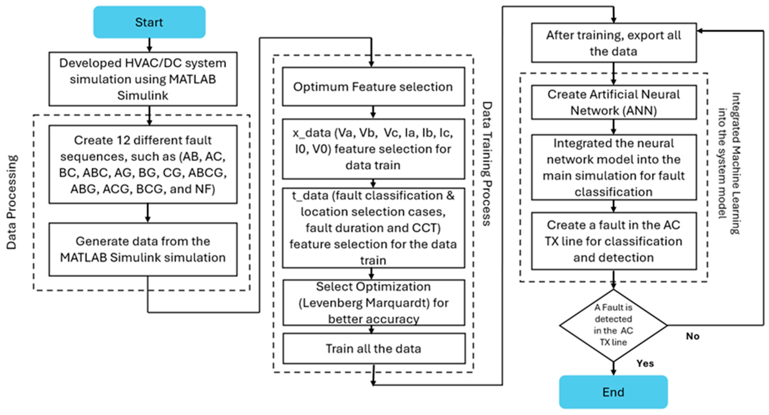
The general structure of the proposed optimized machine learning-based fault detection is depicted in Figure 2. The block diagram represents the overall general process of the proposed fault detection system developed in MATLAB Simulink for an HVAC transmission system. The process begins with building the simulation model and creating twelve different types of fault cases covering single-line, double-line, three-phase, and ground-related disturbances to generate the required voltage and current datasets. The most pertinent features (V_a, V_b, V_c, I_a, I_b, I_c, I₀, and V₀) are subsequently selected from these signals during the data processing stage, along with output parameters including fault classification and location cases, fault duration, and CCT. To improve model performance before training a suitable training optimization algorithm, LM is selected. An ANN optimized model is developed and integrated into the primary Simulink system for real-time fault classification after training. The integrated system is then tested by introducing a failure in the AC transmission line. The process concludes if the ANN finds an error, proving that the machine learning-based classifier was successfully integrated into the simulation environment.

3.1. HVAC Line Model

A simplified HVAC transmission system based on MATLAB Simulink is shown in Figure 3. It consists of a load, a 10 km AC transmission line, and a three-phase source. Bus 1 is connected to the sending end source (G1), while Bus 2 receives power through the transmission line. To evaluate the system performance under fault conditions, a fault is introduced along the transmission line. To analyze fault identification and system behavior in the HVAC network, the receiving end load is connected to Bus 2. The transmission line model nominal parameters are shown in

Table 2. Nominal parameters of the transmission line model.

Parameters	Positive Sequence	Zero Sequence
R(ohms/km)	0.01273	0.3864
L(H/km)	0.933 × 10−3	4.126 × 10−3
C(F/km)	12.74 × 10−9	7.751 × 10−9
Base Power	AC System 1	AC System 2
	100 × 106	100 × 106
AC system voltage	500 KV	345 KV
AC system frequency	60 Hz	60 Hz

.

3.2. Data Processing

Data Generation

Each sample represents a complete fault simulation scenario at a specific fault type and transmission line fault location. For each simulation case, an eight-dimensional feature vector was generated by extracting the RMS magnitudes of the three-phase voltages (V_a, V_b, V_c), three-phase currents (I_a, I_b, I_c), and zero-sequence components (V₀, I₀) from the simulated fault response. A total sample size of 252 was obtained by combining the baseline low impedance fault simulations with additional high-impedance fault simulations generated using fault resistance values of 10 Ω and 50 Ω across the transmission line locations and fault conditions, as shown in

Table 3. Truth table for fault data generation.

No. of Faults	Fault Types	A Line	B Line	C Line	G Line
1	A_G (Phase A to ground)	0	0	0	1
2	B_G (Phase B to ground)	0	0	1	0
3	C_G (Phase C to ground)	0	0	1	1
4	AB_G (double line to ground)	0	1	0	0
5	AC_G (double line to ground)	0	1	0	1
6	BC_G (double line to ground)	0	1	1	0
7	ABC_G (three-phase to ground)	1	0	0	0
8	AB (line to line)	1	0	0	1
9	AC (line to line)	1	0	1	0
10	BC (line to line)	1	0	1	1
11	ABC (three-phase)	0	1	1	1
12	NF	0	0	0	0

. In addition to the baseline low impedance fault simulations, supplementary high-impedance fault scenarios were generated using fault resistance values 10 Ω and 50 Ω to evaluate the robustness under varying fault resistance conditions. From each simulation, one RMS-based feature vector was extracted. Each simulation was run for 0–0.35 s, with the fault being introduced at 0.2 s. Only these electrical features are provided to the ANN as inputs, while the corresponding fault classification and fault location information are used as target outputs. As a result, the model learns the nonlinear relationship between electrical fault signals and fault conditions instead of relying on predefined fault labels or case indices. The considered cases include single line to ground faults (A_G, B_G, C_G), double line to ground faults (AB_G, AC_G, BC_G), three-phase to ground faults (ABC_G), line to line faults (AB, AC, BC), three-phase faults (ABC), and no-fault conditions (NF). These different faults provide a broad range of transient reactions, creating a complete dataset required for precise and accurate fault location detection and classification within the proposed HVAC fault detection system design. Although the dataset size is limited, it is generated systematically through parametric simulation across all fault types and locations along the transmission line. To reduce the risk of overfitting associated with the simulation-generated dataset size, a compact ANN structure with one hidden layer and ten hidden neurons was selected. The dataset was split into subsets for training, validation, and testing. Generalization performance was monitored using the validation and testing results instead of depending only on training accuracy. This ensures comprehensive coverage of operating conditions and fault scenarios, making the dataset suitable for training and evaluating the proposed model.

• Correlation Analysis:

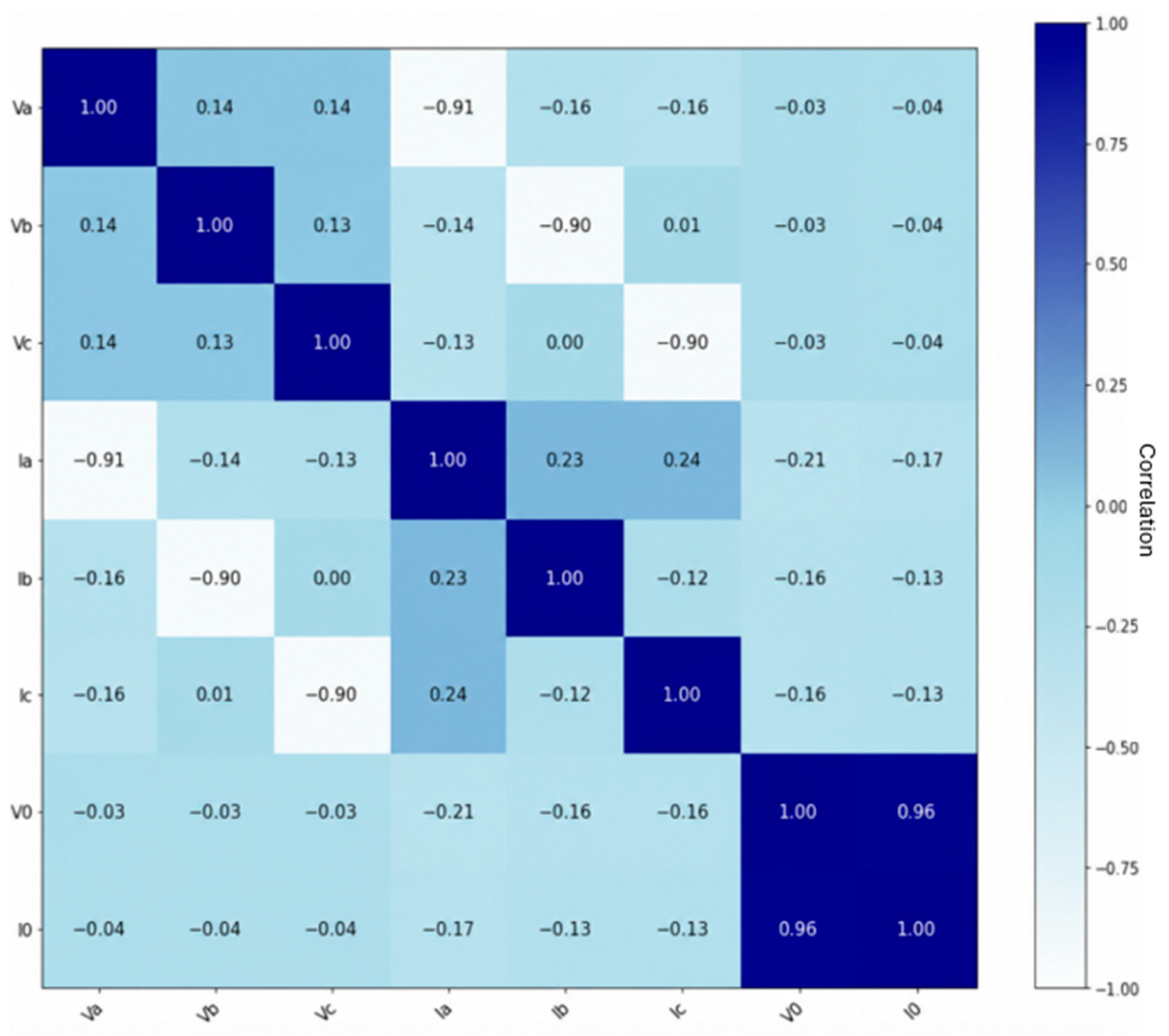
A correlation analysis was performed on all input features to obtain a deeper knowledge of the data inside the dataset. The results are shown in Figure 4. With coefficients ranging from −1 to +1, where +1 indicates a perfect positive linear relation, −1 indicates a perfect negative linear relationship, and 0 indicates no linear correlation, the correlation matrix quantifies the linear dependence between each pair of variables. Each feature shows a perfect self-correlation of 1.0 along the main diagonal as predicted. There are significant interdependencies between several feature pairs. The most important negative correlations are (V_a–I_a = −0.91, V_b–I_b = −0.90, V_c–I_c = −0.90) between phase voltages and the corresponding phase currents are particularly notable. These correlations demonstrate the inverse dynamic link between voltage and current during fault conditions. In a similar vein, the zero-sequence component synchronized behavior under unbalanced fault conditions is highlighted by their strong positive correlation (V₀–I₀ = 0.96). The majority of the remaining feature pairs show weak correlations, indicating that the dataset includes a wide range of independently correlated electrical characteristics across phases. The presence of feature groups with both high and weak correlations confirms the effectiveness of the chosen variables in capturing the underlying electrical activity under various fault conditions. Due to their balanced variability, the features are highly suitable for training ML models for precise and reliable fault identification as they provide sufficient discriminative information.

• Sensitive Analysis:

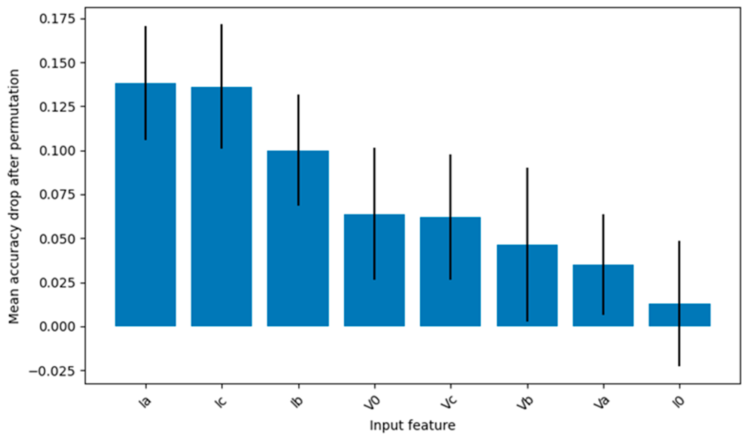
Sensitivity analysis was used to evaluate the comparative impact of each input feature on the model’s fault classification and location performance. Permutation feature significance was used to shuffle each variable separately while keeping the others fixed. The resulting decline in model accuracy was evaluated. As shown in Figure 5, the three-phase currents (I_a, I_b, and I_c) create the greatest accuracy drop, indicating that current components carry the most prevalent fault signs in the HVAC transmission line. The moderate sensitivity of the zero-sequence features (V₀, I₀) indicates their relevance in identifying unbalanced and ground-related faults. Comparatively, the phase voltages (V_a, V_b, and V_c) have less impact and provide useful but not crucial information. Overall, the research indicates that the chosen feature set is appropriate and that current-based parameters are crucial for accurate and reliable fault detection.

3.3. Data Training Process

3.3.1. Feature Selection

The dataset has [252 × 8] ‘xdata’ input variables and [252 × 5] ‘tdata’ output variables observations in total, as shown in

Table 4. The recorded first five xdata of input variables.

Number	Va	Vb	Vc	Ia	Ib	Ic	V0	I0
0	0.765264	0.765275	0.765286	4.698692	4.699217	4.699353	1.000000 × 10−10	5.260000 × 10−9
1	0.000541	0.750604	0.756007	49.105832	7.961843	8.200031	3.485646 × 10−1	1.632792 × 101
2	0.763451	0.000534	0.753397	8.440489	48.503182	7.672964	3.483375 × 10−1	1.626101 × 101
3	0.752875	0.755574	0.000540	7.978014	8.089689	48.975285	3.490605 × 10−1	1.642476 × 101
4	0.000619	0.000611	0.748005	65.784434	65.784434	5.118487	3.524653 × 10−1	1.655032 × 101

and

Table 5. The recorded first five tdata of output variables.

Number	A	B	C	G	Length in km
0	0	0	0	0	10
1	0	0	0	1	10
2	0	0	1	0	10
3	0	0	1	1	10
4	0	1	0	0	10
5	0	1	0	1	10

. The dataset was randomly divided into training (70%), validation (15%), and testing (15%) subsets to ensure reliable model evaluation and generalization. The three-phase voltages (V_a, V_b, and V_c), three-phase currents (I_a, I_b, and I_c), and zero-sequence components (V₀, I₀) that together describe the dynamic electrical response of the HVAC transmission line under both normal and faulted operating conditions in the ‘xdata’. These input features correspond to RMS magnitudes extracted from each simulated fault condition and are used to characterize the electrical fault signal provided to the ANN. The fault identification parameters are represented in the ‘tdata’ outputs, where each sample indicates different faulty cases associated with fault position in kilometers along with the transmission line. Assuring that all fault results are consistently represented, these outputs are constructed in accordance with the truth table standards listed in Table 4.

3.3.2. Fault Classification and Location Selection Cases

The AC transmission line of the proposed model was utilized to systematically develop numerous fault types to provide plenty of faulty cases for both location detection and identification. In this model, the AC line was divided into 1 km to 10 km lengths to ensure a uniform distribution of possible fault points along the line. To create the training dataset, all chosen fault types (V_a, V_b, V_c, I_a, I_b, I_c, V₀, I₀) were consecutively simulated at each 1 km interval, and corresponding voltage and current signals were recorded. To ensure accuracy, each case was simulated with a fixed fault resistance of 0.01 Ω and a ground resistance of 0.001 Ω, as shown in

Table 6. Fault pattern generation.

No. of Patterns	Parameters	Set Values
1	Fault Types	Va, Vb, Vc, Ia, Ib, Ic, V0, I0
2	Fault Resistance	Case 1: 1, 2, 3, …… 10 km Case 2: 1, 2, 3, …… 10 km Case 3: 1, 2, 3, …… 10 km …… Case 10: 1, 2, 3, …… 10 km
3	Ground Resistance	0.001 Ω
4	Fault Resistance	0.01 Ω, 10 Ω, 50 Ω

. To address the high-impedance fault issue, more simulations were conducted with higher fault resistance values of 10 Ω and 50 Ω while maintaining the ground resistance constant at 0.001 Ω. These additional cases were included in the expanded dataset to assess the proposed ANN framework in both low-impedance and high-impedance fault scenarios. This systematic procedure produced a comprehensive database of different faulty cases that efficiently facilitate precise fault location detection and accurate fault identification.

The fault position along the AC line is used to train each case, with each 1 km representing a distinct identification and location detection in km length. As an example, Case 1 corresponds to a fault occurring at the 1 km out of 10 km point, and all 12 fault types are generated and trained for this location, as shown in

Table 7. Different types of fault identification and location detection case selection.

SL. No.	Case	Types of Faults	Fault Classification
			A	B	C	G	Length in km
1	1	NF	0	0	0	1	10
2		A_G	0	0	1	0	10
3		B_G	0	0	1	1	10
4		C_G	0	1	0	0	10
5		AB_G	0	1	0	1	10
6		AC_G	0	1	1	0	10
7		BC_G	0	1	1	1	10
8		ABC	1	0	0	0	10
9		ABC_G	1	0	0	1	10
10		AB	1	0	1	0	10
11		AC	1	0	1	1	10
12		BC	0	0	0	0	10
13	2	NF	0	0	0	1	9
14		A_G	0	0	0	1	9

. Similarly, case 2 represents the 2 km out of 10 km point, Case 3 represents the 3 km out of 10 km point, continuing up to Case 10 at 10 km, ensuring that every kilometer segment contains a complete set of fault patterns for effective training and validation.

3.3.3. Critical Clearing Time (CCT)

In this study, the fault timing parameters obtained from ANN-based fault classification and location detection are used to calculate Critical Clearing Time (CCT), an ML-integrated fault clearing time indicator. The proposed formulation uses the detected fault initiation time and fault clearing duration to estimate the fault persistence period associated with each simulated fault condition. This approach is different from the conventional transient stability definition of CCT, which is often obtained by rotor angle dynamics, swing-equation analysis, or equal area criterion-based stability assessment. By providing additional timing information that might assist with protection-oriented decision making, this evaluation improves the fault classification and location prediction process. The proposed CCT is measured as the duration for which the fault persists on the transmission line before clearing.

$$\mathrm{CCT}={\mathrm{T}}_{\mathrm{f}\mathrm{d}}-{\mathrm{F}}_{\mathrm{s}\mathrm{t}}$$

(1)

Equation (1), where ‘${\mathrm{T}}_{\mathrm{f}\mathrm{d}}$’ represents total fault duration and ‘${\mathrm{F}}_{\mathrm{s}\mathrm{t}}$’ represents fault starting time. Calculating the time difference between these two parameters yields CCT. This expression represents the estimated fault persistence interval derived from the predicted fault timing parameters. The computed value is used as a comparative fault timing index within the proposed ANN framework to support a protection-oriented stability assessment under various HVAC transmission line fault conditions.

Table 8. CCT calculation of twelve different types of faults.

SL. No.	Fault Types	Tfd	Fst	CCT
1	A_G	0.4	0.3901	0.0099
2	B_G	0.4	0.2053	0.1947
3	C_G	0.4	0.2064	0.1963
4	AB_G	0.4	0.2139	0.1861
5	AC_G	0.4	0.2089	0.1911
6	BC_G	0.4	0.2022	0.1978
7	AB	0.4	0.2021	0.1979
8	AC	0.4	0.2066	0.1934
9	BC	0.4	0.2018	0.1982
10	ABC	0.4	0.2016	0.1984
11	ABC_G	0.4	0.2014	0.1986
12	NF	0.4	0	0

presents the CCT values for the twelve simulated fault conditions.

3.3.4. Optimization Algorithm Selection for ANN Training

The optimization algorithms investigated for the proposed ANN framework are presented in

Table 9. ANN training optimization model selection.

SL. No.	Optimizer	Algorithm Type	Advantage	ANN Characteristics	Performance Metrics
1	Bayesian Regularization (BR)	Regularization based	Moderate generalization capability. Reduces overfitting by automatically adjusting the effective number of parameters.	Input neurons: 8 Hidden neurons: 10 Output neurons: 5 Activation (hidden): tansing Activation output: purelin Data division: train (70%), test (15%), and validation (15%).	Mean Squared Error (MSE) Regression Coefficient (R)
2	Scaled Conjugate Gradient (SCG)	Conjugate gradient-based	Faster than simple gradient descent. Memory efficient. Good for medium-sized networks.	Input neurons: 8 Hidden neurons: 10 Output neurons: 5 Activation (hidden): tansing Activation output: purelin Data division: train (70%), test (15%), and validation (15%).	Mean Squared Error (MSE) Regression Coefficient (R)
3	Levenberg–Marquardt (LM)	Second order (quasi-newton method)	Very fast convergence. High accuracy for moderately sized problems. Suitable for noisy training data.	Input neurons: 8 Hidden neurons: 10 Output neurons: 5 Activation (hidden): tansing Activation output: purelin Data division: train (70%), test (15%) and validation (15%).	Mean Squared Error (MSE) Regression Coefficient (R)

. Following a comparative evaluation of the optimization strategies, ANN training characteristics, and performance metrics, Levenberg–Marquardt (LM) achieved the best overall performance and was therefore selected as the training optimizer for the proposed model.

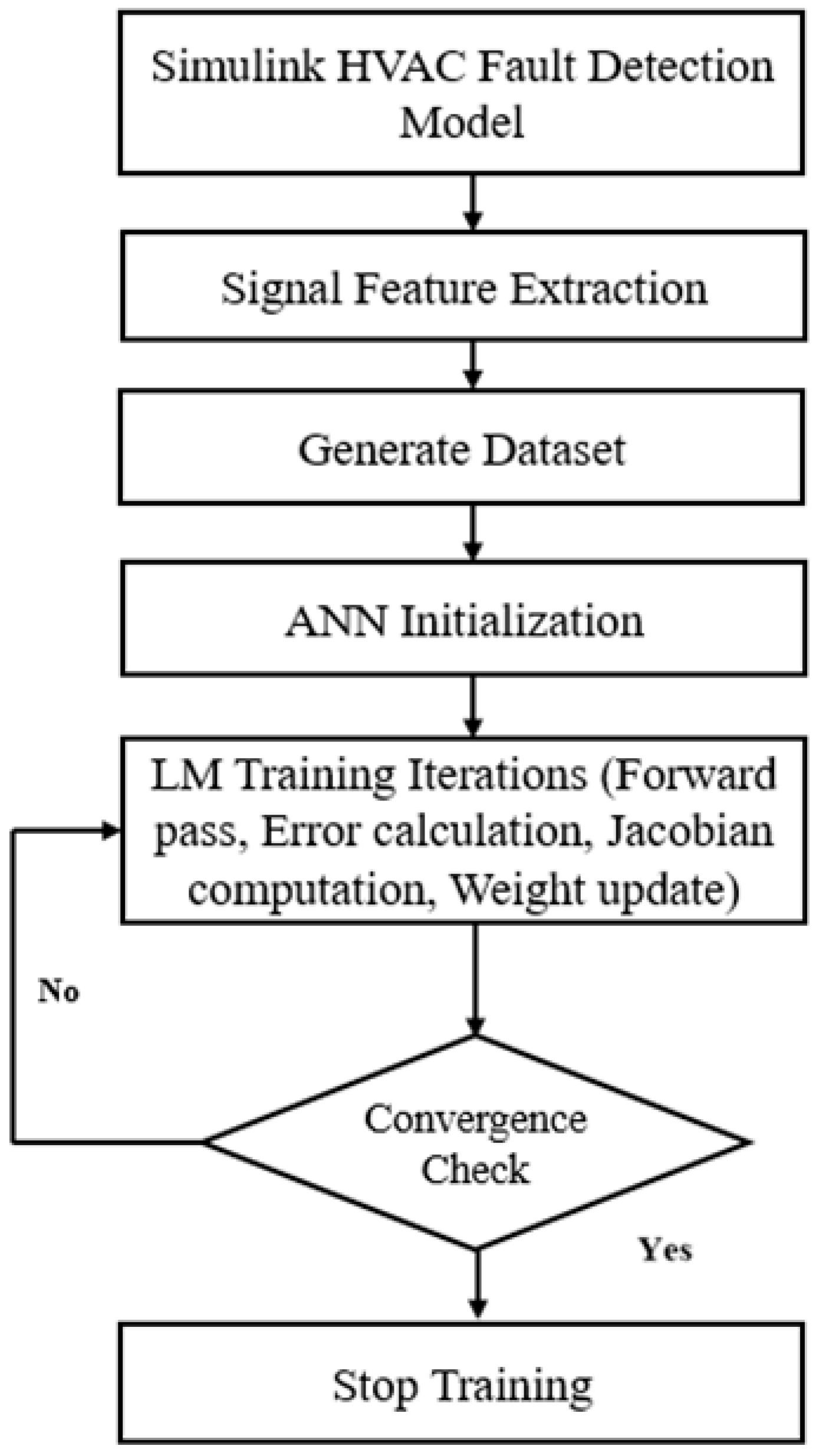
The machine learning model created for fault classification and location detection in the HVAC transmission system is trained primarily using the Levenberg–Marquardt (LM) optimization algorithm. To ensure precise learning and quick convergence, a highly effective optimization method is necessary since the voltage and current patterns produced during fault circumstances have nonlinear and dynamic features. When it comes to training nonlinear regression and classification models, the LM algorithm performs better than traditional gradient-based techniques, making it an optimal choice for these types of applications [24]. Figure 6 flowchart illustrates the LM optimization process for training the ANN in HVAC transmission line fault detection.

The LM algorithm iteratively improves the model weights during training to reduce the mean squared error (MSE) between the actual target values produced from simulation instances and the expected outputs (types of faults and location). LM functions as a hybrid between the gradient descent approach and the Gauss–Newton algorithm. When the model is far from convergence, LM maintains stability by acting like gradient descent as the error drops and the solution gets closer to the optimal region. LM shifts toward the Gauss–Newton update, greatly speeding up convergence. High learning efficiency and robustness are guaranteed by this adaptive method.

$$\mathrm{e}=\mathrm{t}-\mathrm{y}$$

(2)

Equation (2) describes the input and output training set of the network error vector ‘e’, ‘t’ is the target vector, and ‘y’ is the ANN output.

$$\mathrm{E}(\mathsf{\theta })={\displaystyle \frac{1}{2}}{\displaystyle {\sum }_{\mathrm{i}=1}^{\mathrm{n}}}{\mathrm{e}}_{\mathrm{i}}^2$$

(3)

In Equation (3), ‘E’ represents the overall error to be minimized, where ‘θ’ is the weights and biases of the ANN, ‘n’ is the total number of samples, and ‘${\mathrm{e}}_{\mathrm{i}}$’ is the error of the ${\mathrm{i}}^{\mathrm{t}\mathrm{h}}$ sample.

$$\mathrm{J}\left(\mathsf{\theta }\right)=\left[{\displaystyle \frac{{\partial }_{\mathrm{e}\mathrm{i}}}{{\partial }_{\mathsf{\theta }\mathrm{j}}}}\right]$$

(4)

The Jacobian matrix, which contains the partial derivatives of the network errors with respect to the model parameters, is denoted by Equation (4). Equations (5) and (6) provide a Gauss–Newton approximation of the Hessian matrix and the corresponding gradient vector used in the LM optimization process.

$${\mathrm{H}}_{\mathrm{k}}\approx {\mathrm{J}}_{\mathrm{k}}^{\mathrm{T}}{\mathrm{J}}_{\mathrm{k}}$$

(5)

$${\mathrm{g}}_{\mathrm{k}}={\mathrm{J}}_{\mathrm{k}}^{\mathrm{T}}{\mathrm{e}}_{\mathrm{k}}$$

(6)

$${\mathsf{\theta }}_{\mathrm{K}+1}={\mathsf{\theta }}_{\mathrm{K}}-{\left({\mathrm{j}}_{\mathrm{T}}^{\mathrm{K}}{\mathrm{j}}_{\mathrm{K}}+\mathsf{\lambda }\mathrm{I}\right)}^{-1}{\mathrm{j}}_{\mathrm{T}}^{\mathrm{K}}{\mathrm{e}}_{\mathrm{K}}$$

(7)

Equation (7) describes the LM optimization algorithm used to train neural networks, where ‘${\mathsf{\theta }}_{\mathrm{k}}$’ represents the current weight and bias vector, ‘${\mathrm{J}}_{\mathrm{k}}$’ denotes the Jacobian matrix, ‘${\mathrm{e}}_{\mathrm{k}}$’ represents the error vector, ‘${\mathrm{H}}_{\mathrm{k}}$’ denotes the Hessian matrix approximation, ‘${\mathrm{g}}_{\mathrm{k}}$’ is the gradient vector, ‘λ’ is the damping factor, and ‘I’ denotes the identity matrix. During training, MATLAB automatically modifies the damping factor ‘λ’. A smaller ‘λ’ enables faster Gauss–Newton convergence, while a larger ‘λ’ makes the update more conservative, such as gradient descent [24].

3.4. Artificial Neural Network (ANN) Based Fault Classification and Detection

3.4.1. Input and Output Selection

Selecting the appropriate network size and structure depends directly on the number of input and output parameters required for accurate fault analysis. Although a smaller number of inputs leads to a more concise network, the model must still receive enough information to fully represent the system’s electrical behavior. The inputs used in this model are the fundamental (50 Hz) magnitudes of the three-phase voltages and three-phase currents measured at one end of each transmission line section, ensuring that the essential characteristics of every fault condition are captured. There are five defined outputs for the output layer: One output indicates if the neutral (ground) path is involved in the fault loop, three outputs indicate whether phases A, B, or C are active in the fault, and one output indicates where it is located along the transmission line. The input vector ‘X’ and the target output vector ‘T’, where ‘T’ encodes the associated fault type and location, and ‘X’ contains the voltage and current features, are used to operate the whole fault classification network as shown in Equations (8) and (9).

$${\mathrm{x}}_{\mathrm{d}\mathrm{a}\mathrm{t}\mathrm{a}}=\left[{\mathrm{V}}_{\mathrm{a}}{\mathrm{V}}_{\mathrm{b}}{\mathrm{V}}_{\mathrm{c}}{\mathrm{I}}_{\mathrm{a}}{\mathrm{I}}_{\mathrm{b}}{\mathrm{I}}_{\mathrm{c}}{\mathrm{V}}_0{\mathrm{I}}_0\right]$$

(8)

$${\mathrm{t}}_{\mathrm{d}\mathrm{a}\mathrm{t}\mathrm{a}}=\left[\mathrm{A},\mathrm{B},\mathrm{C},\mathrm{G},\mathrm{L} (\mathrm{l}\mathrm{o}\mathrm{c}\mathrm{a}\mathrm{t}\mathrm{i}\mathrm{o}\mathrm{n}/\mathrm{k}\mathrm{m})\right]$$

(9)

Since the target vector consists of four binary fault signals (A, B, C, and G) and one continuous location variable (L), a unified mean squared error (MSE) loss function is applied over the entire output vector during ANN training. Before training, the input and target variables are scaled to a similar numerical range using MATLAB’s automatic map minmax preprocessing to adjust for this mixed target structure. This prevents the continuous location output from taking over the binary fault classification outputs during MSE computation. After predicting the location, the output is interpreted in its original kilometer scale. No additional weight factors were assigned to the individual’s output variables. Therefore, the MSE was computed simultaneously across all five outputs [25].

$$\mathrm{M}\mathrm{S}\mathrm{E}={\displaystyle \frac{1}{\mathrm{N}\times 5}}{\displaystyle \sum _{\mathrm{i}=1}^{\mathrm{N}}}{\displaystyle \sum _{\mathrm{j}=1}^5}{\left({\mathrm{T}}_{\mathrm{i}\mathrm{j}}-{\mathrm{y}}_{\mathrm{i}\mathrm{j}}\right)}^2$$

(10)

In Equation (10), ‘$\mathrm{N}$’ represents the total number of samples, ‘5’ denotes the number of output variables, ‘${\mathrm{T}}_{\mathrm{i}\mathrm{j}}$’ is the target value and ‘${\mathrm{y}}_{\mathrm{i}\mathrm{j}}$’ is the ANN predicted value.

3.4.2. Structure of the ANN-Based Fault Classification

After selecting a sufficient number of input and output parameters, the Artificial Neural Networks (ANN) architectural design was optimized by selecting an optimal number of layers and neurons per layer. Through iterative testing with various network setups, the size of the hidden layers was empirically chosen. A three-layer feed-forward ANN with 8 neurons in the input layer, 10 neurons in the hidden layer, and 5 neurons in the output layer was identified to provide the best results after numerous trials, as shown in Figure 7. The compact single hidden layer structure was selected to limit model complexity and reduce the possibility of overfitting, considering the simulation-generated dataset. The hyperbolic tangent sigmoid activation function, which produces smooth, continuous outputs and allows the network to generate complex decision boundaries in a high-dimensional feature space, was used in the hidden layer to guarantee efficient nonlinear mapping. In fault classification analysis, this quality is crucial for attaining strong generalization. A saturating linear (SatLin) transfer function was used for the output layer in order to generate bounded outputs that corresponded to the desired binary fault indicators. Each output neuron is trained to produce a logical ‘0’ or ‘1’ depending on the type of problem that is occurring in the system. This enables precise multi-class fault identification.

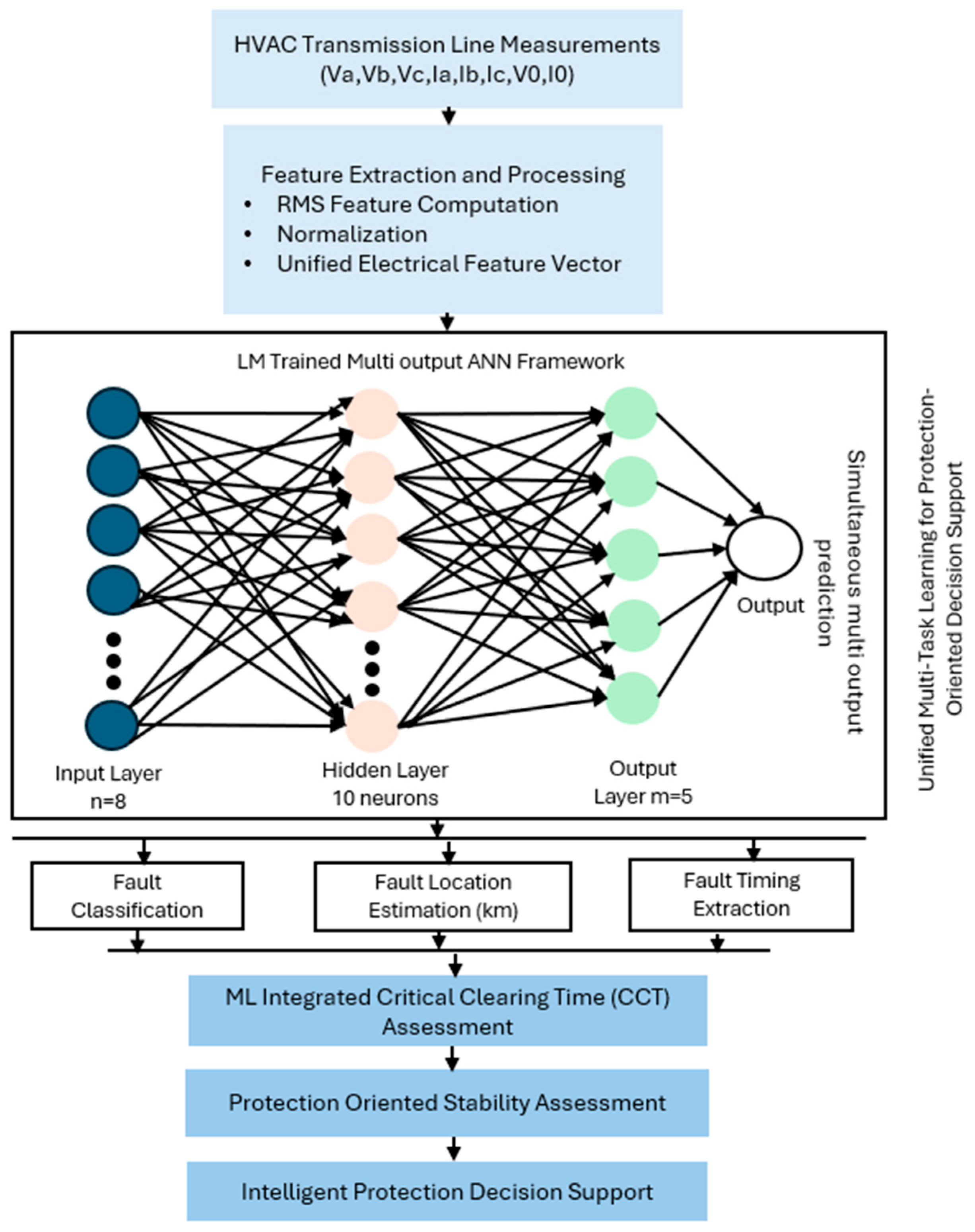
Figure 8 shows the general structure of the proposed unified intelligent protection framework. First three-phase voltage, current, and zero-sequence electrical observations are converted into a single electrical feature representation using RMS feature extraction and normalization. The LM-trained multi-output ANN simultaneously predicts fault timing parameters, fault location estimates, and fault classification from the shared feature representation. The estimated fault timing parameters for ML-integrated CCT assessment enable protection-oriented stability assessment and intelligent protection decision support inside a single unified framework.

3.4.3. Training Performance Evaluation

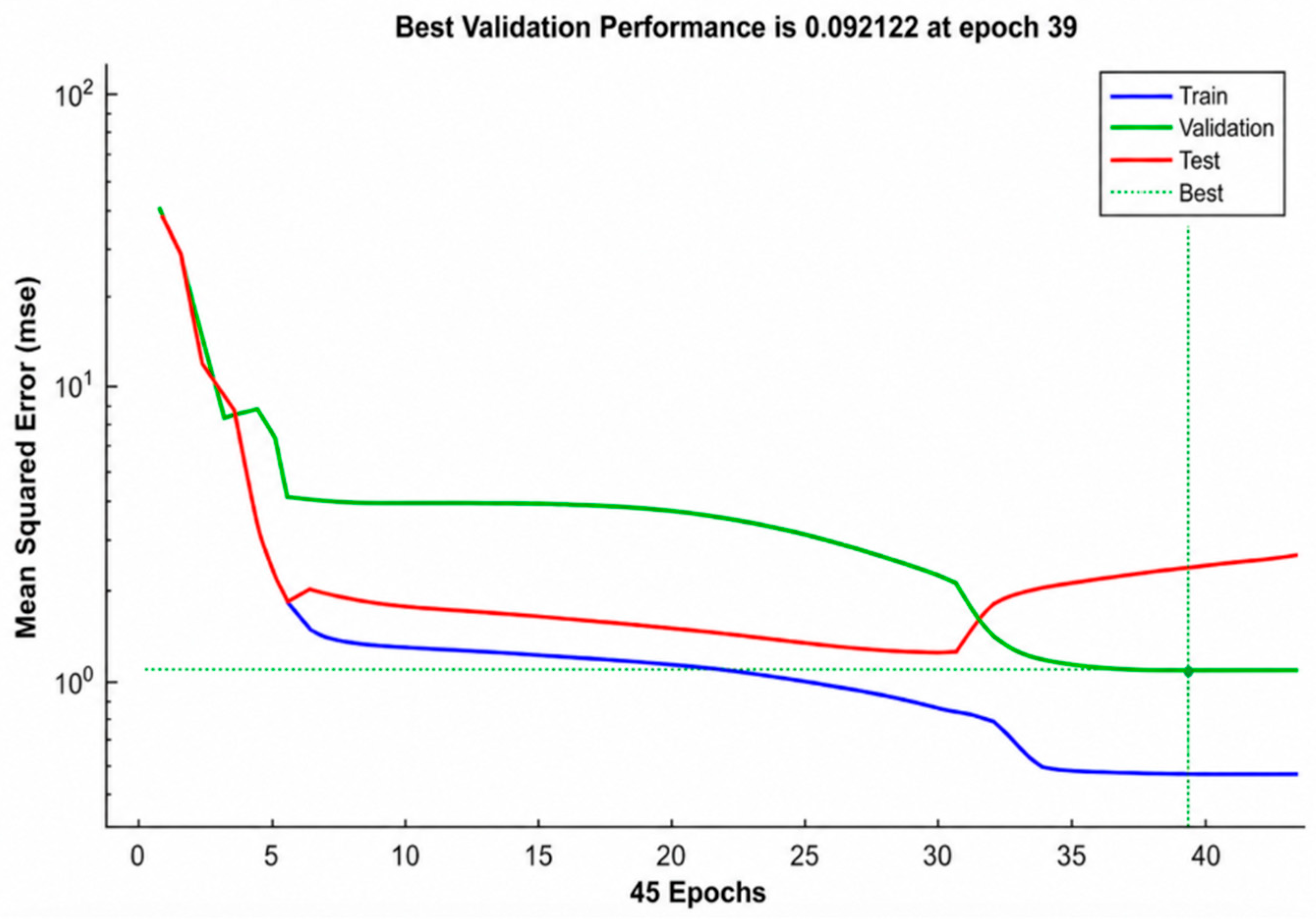
The training performance curve is illustrated in Figure 9. A significant decrease in MSE in the early epochs indicates that learning is successful and the network quickly adjusts to the fault-based anomalies. The validation curve confirms that there is no early overfitting, and the model retains appropriate generalization by exhibiting a similar trend in the early phase. This behavior indicates that the LM learning rule is operating as intended, effectively reducing the error using its second-order optimization technique. The quick decrease further illustrates how LM provides very fast convergence, allowing the network to arrive in an ideal area of the solution space in fewer epochs. Overall, the performance trajectory validates the suitability of the LM algorithm for the proposed fault classification method.

4. Results Analysis

A thorough analysis of the proposed LM-optimized ANN framework for fault analysis of HVAC transmission systems is provided in this section. It comprises per-kilometer fault location estimation, thorough performance validation of fault detection and classification, and stability assessment based on CCT under various fault scenarios. After analyzing quantitative metrics, including regression coefficient, mean squared error, and classification outputs, a comparison with traditional and modern fault detection techniques is conducted to demonstrate the practical benefits and real-time applicability of the proposed technique.

4.1. Fault Detection in HVAC System

This section demonstrates different testing results of the LM-optimized ANN-based fault classification model. The analysis emphasizes the neural network’s capability to accurately classify faults, along with its precision and overall dependability in identifying the correct anomaly condition. The accuracy and consistency of the neural network model are validated using key performance metrics such as the correlation coefficient (R), mean squared error (MSE), and the corresponding training, validation, and testing performance.

Table 10. Neural networks training model dataset.

Parameters	Observations	MSE	R
Training	84	0.0320	0.9973
Validation	18	0.0921	0.9925
Test	18	0.2384	0.9831

presents the neural network model training dataset.

• Test Result of Single Phase to Ground Fault Case-1:

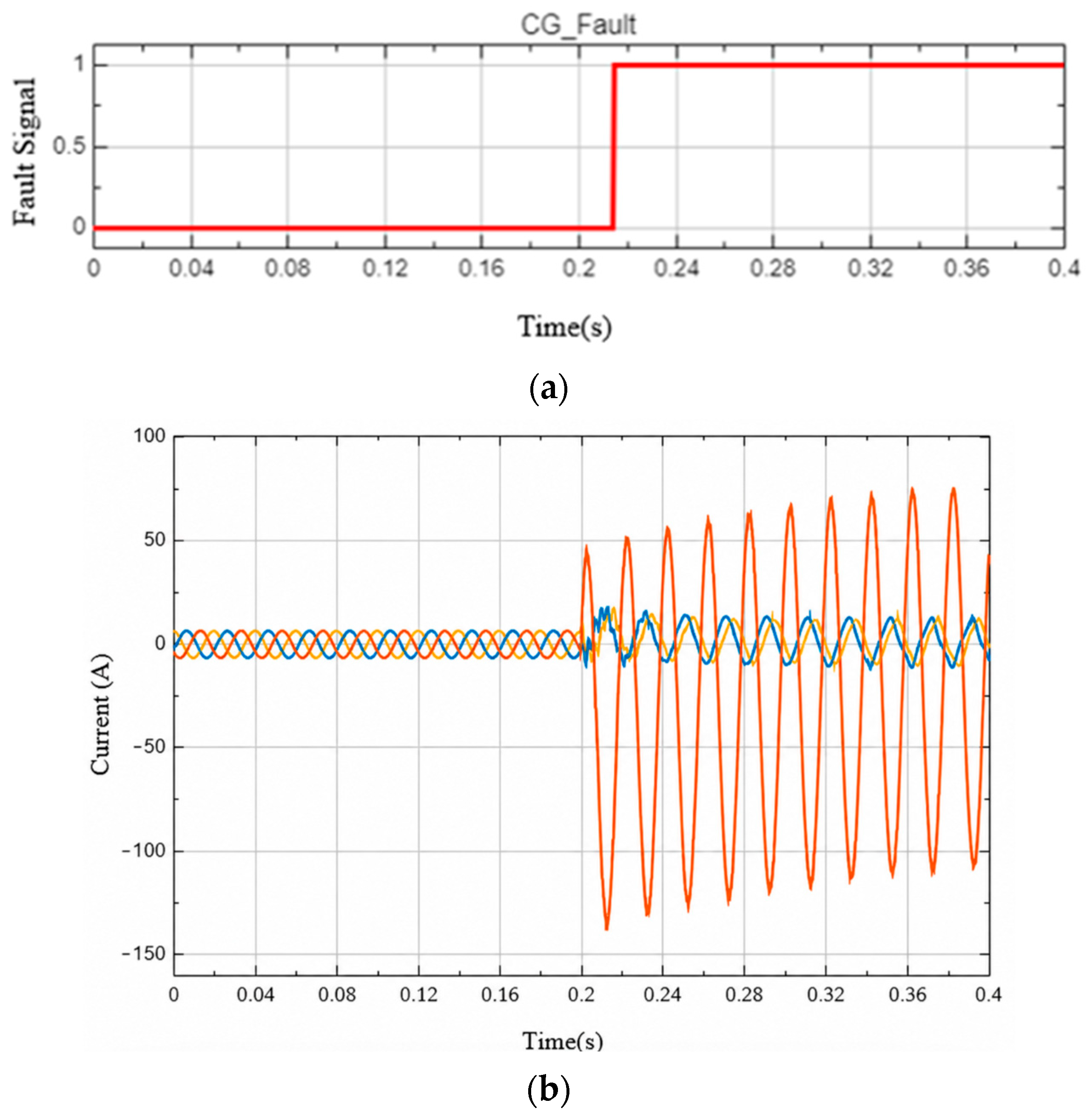
Figure 10a illustrates the simulated single line to ground (CG) fault occurring at 2.197 km along the transmission line. The fault is initiated at 0.2064 s, where the CG fault signal shifts quickly from 0 to 1, confirming the onset of the disturbance. The fault continues active for a length of 0.1937 s, after which the signal drops to zero, signaling fault clearance. To train and test the performance of the ANN-based classification model, this binary representation efficiently displays the precise starting point and clear instances of the CG fault.

For the same CG fault, the three-phase current response is shown in Figure 10b. Prior to the fault, all phases indicate balanced sinusoidal currents. Phases A and B (yellow and blue) become distorted when the system faces an unbalanced condition, while Phase C (red) shows a sudden spike in magnitude immediately following the fault start because of its direct connection to ground. These brief oscillations and the notable increase in Phase C current clearly demonstrate how the CG fault affects system dynamics.

• Test Result of Double Phase to Ground Fault Case-2:

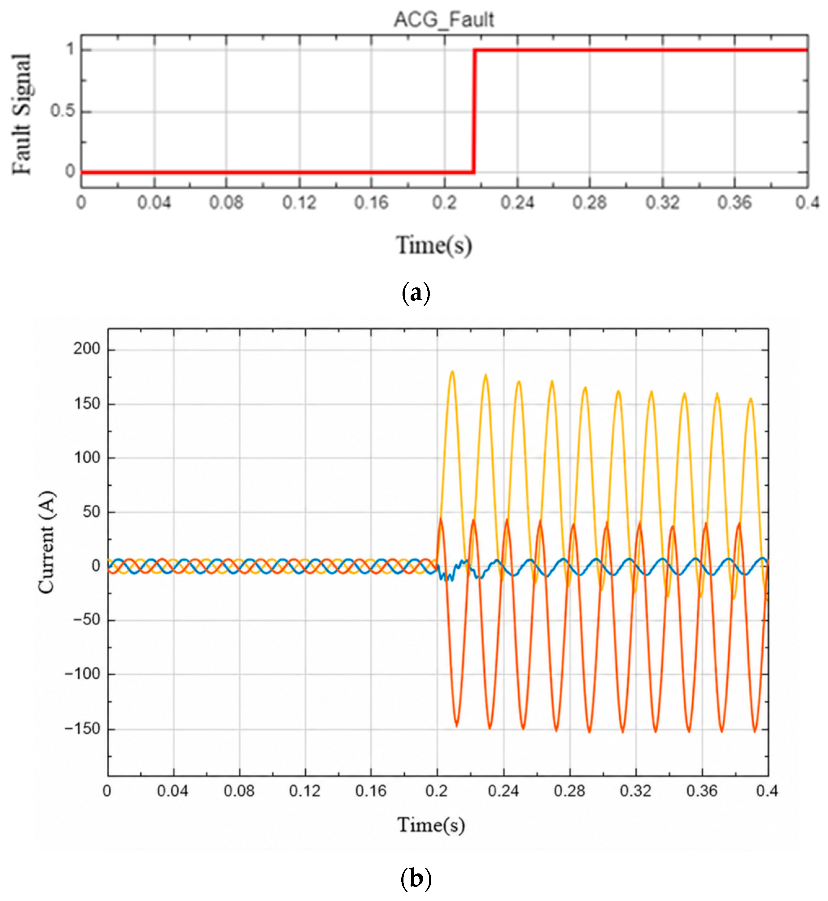
The simulated AC_G double line to ground fault that occurred 2.777 km along the transmission line is shown in Figure 11a. The AC_G fault signal rapidly shifts from 0 to 1 at 0.2089 s, identifying the precise start of the abnormality. The signal returns to zero, indicating total fault clearance, when the fault is active for about 0.191 s.

In the same AC_G fault, Figure 11b illustrates the three-phase current response, where all phases indicate sinusoidal currents that are in balance. When the system is in an unbalanced condition, Phases A and C (yellow and red) become distorted, while Phase B (blue) shows a sharp increase in amplitude just after the fault begins due to its direct connection to ground. These fleeting oscillations and the significant rise in Phase AC current make it clear how the AC_G fault impacts the dynamics of the system.

• Test Result of Phase-to-Phase Fault Case-3:

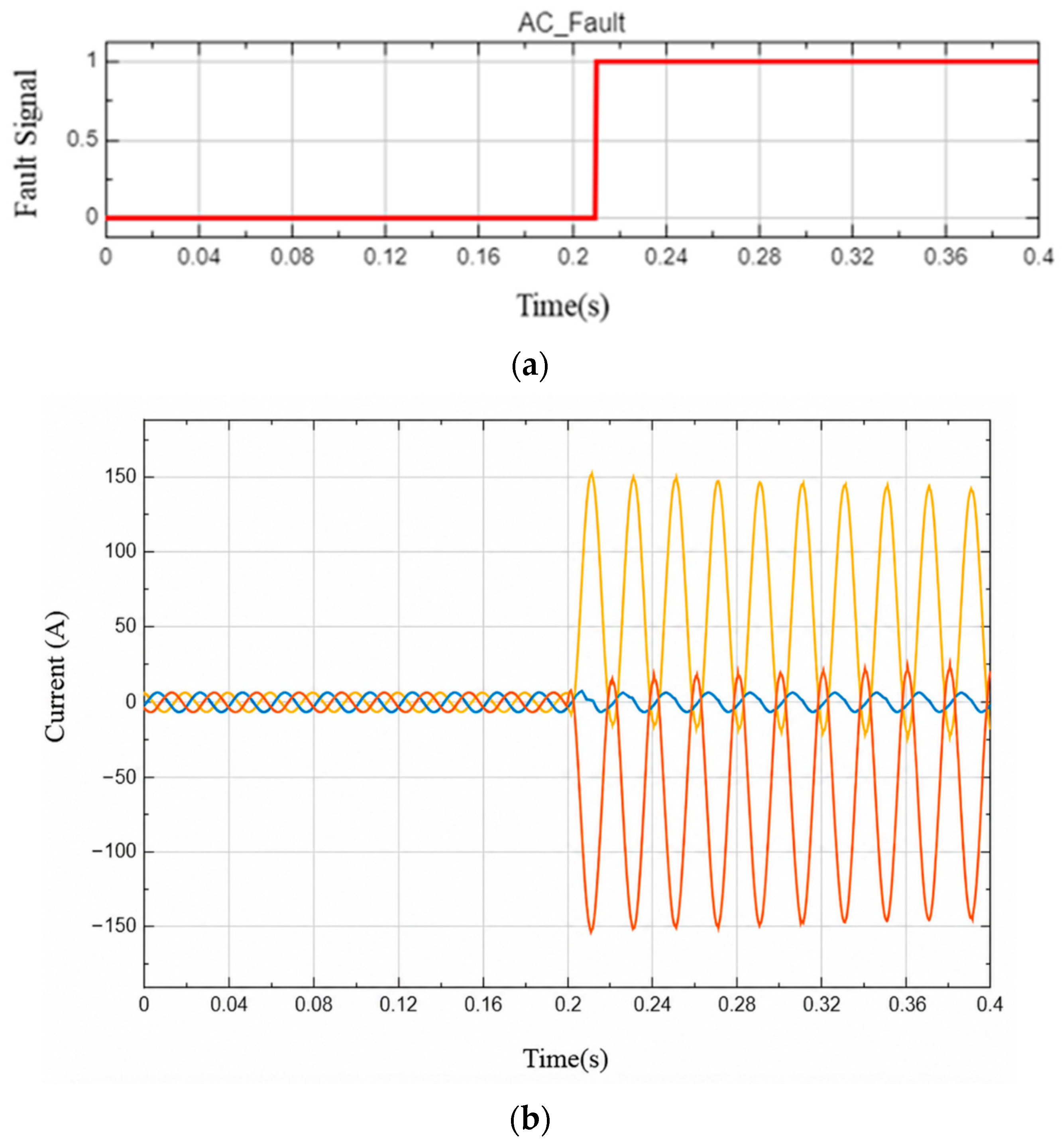
Figure 12a depicts the simulated AC double-phase-to-phase fault that occurred at 1.583 km along the transmission line. At 0.2066 s, the AC fault signal promptly shifts from 0 to 1, indicating the exact start of the anomaly. After the fault is active for around 0.1935 s, the signal returns to zero, indicating the complete fault clearance.

The phase-to-phase current response is shown in Figure 12b, where each phase shows balanced sinusoidal currents. Phases A and C (yellow and red) become distorted when the system is not in balance, while Phase B (blue) displays a rapid spike in amplitude right after the fault. It is clear how the fault impacts the system’s dynamics from these transient oscillations and the notable increase in Phase AC current.

• Test Result of Three Phase to Ground Fault Case-4:

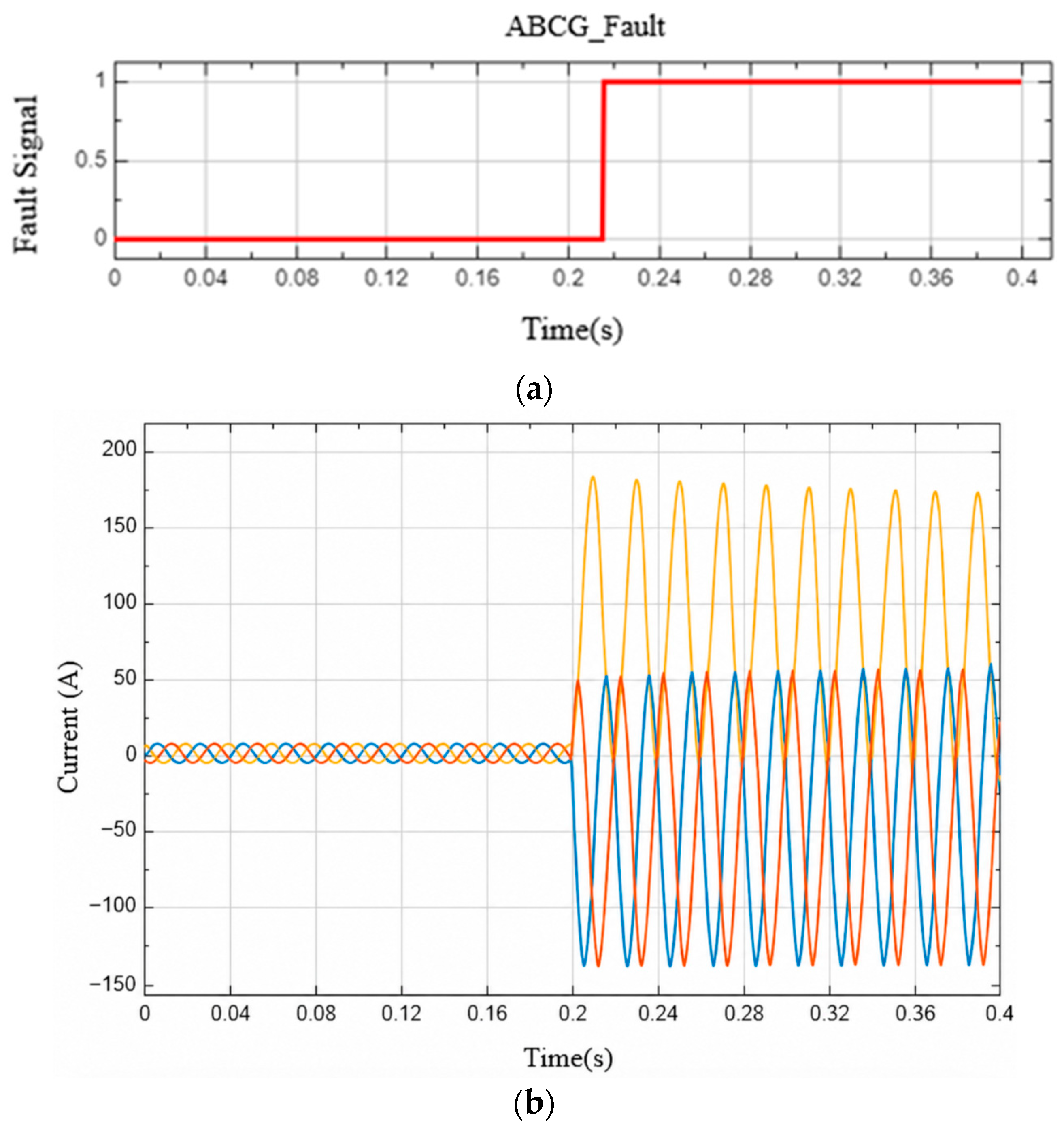
The simulated ABC_G Three Phase to Ground fault, which happened at 0.7285 km along the transmission line, is shown in Figure 13a. The ABC fault signal quickly changes from 0 to 1 at 0.2018 s, indicating the precise beginning of the anomaly. The signal returns to zero, denoting full fault clearance, when the fault is active for about 0.1982 s. It is noticeable from these brief oscillations and the notable increase in Phase ABC current how the ABC_G fault impacts the system’s dynamics.

The three-phase currents at the faulted area during an ABC to ground fault are shown in Figure 13b. The three-phase currents show a normal balanced sinusoidal pattern before the fault (up to about 0.206 s). Due to the simultaneous short circuit of all phases to ground, the ABC_G fault causes all three-phase currents to abruptly increase in magnitude and become significantly twisted. As a result, the waveform shows a strong symmetrical fault current with notable oscillations during the course of the fault. The graph clearly illustrates the change from regular operation to the highly distorted, high-magnitude currents linked to a three-phase to ground fault.

To provide a result-based justification for selecting the Levenberg–Marquardt (LM) training algorithm, the same ANN architecture was trained using different optimization algorithms, including Bayesian Regularization (BR), Scaled Conjugate Gradient (SCG), and LM. During this comparison, the input features, output targets, hidden layer size, and (training, validation, testing) data division were kept unchanged to ensure a fair evaluation. As shown in

Table 11. Performance comparison of different ANN training algorithms.

Training Algorithm	Training MSE	Validation MSE	Test MSE	Training R	Validation R	Test R	Epochs
BR	0.2354	0.1320	0.4637	0.9658	0.9768	0.9645	92
SCG	0.2655	0.1460	0.4287	0.9793	0.9803	0.9628	82
LM	0.0320	0.0921	0.2384	0.9973	0.9925	0.9831	45

, the LM-trained ANN converged in 45 epochs, where SCG and BR required 82 and 92 epochs, respectively. In addition to requiring fewer epochs, LM achieved the lowest training MSE, validation, and test MSE with values of 0.0320, 0.0921, and 0.2384, respectively. It also produced the highest training R, validation, and test R values of 0.9973, 0.9925, and 0.9831. These results confirm that LM provides better convergence and prediction accuracy than BR and SCG for the proposed multi-output ANN framework. Therefore, the LM algorithm was selected as the final ANN training optimizer for the proposed framework, providing accurate fault classification, fault location estimation, fault timing extraction, and ML-integrated CCT assessment within a single prediction model.

4.2. Performance Evaluation Under High-Impedance Fault Conditions

The proposed LM-trained ANN was further assessed with fault resistance values of 10 Ω and 50 Ω in addition to the baseline 0.01 Ω case, with the grounding resistance set at 0.001 Ω to assess model robustness under high-impedance fault conditions. This study is crucial because higher fault resistance makes fault classification and location estimation more difficult by lowering the fault current magnitude and altering the voltage current pattern. The ANN obtained MSE values of 0.0321, 0.0593, and 0.0409 for training, validation, and testing after retraining using the combined 252-case dataset. The corresponding R values were 0.9329, 0.8758, and 0.9153. These findings show that the proposed framework has adequate prediction capability under various fault resistance conditions, despite the fact that high-impedance faults increase signal variability.

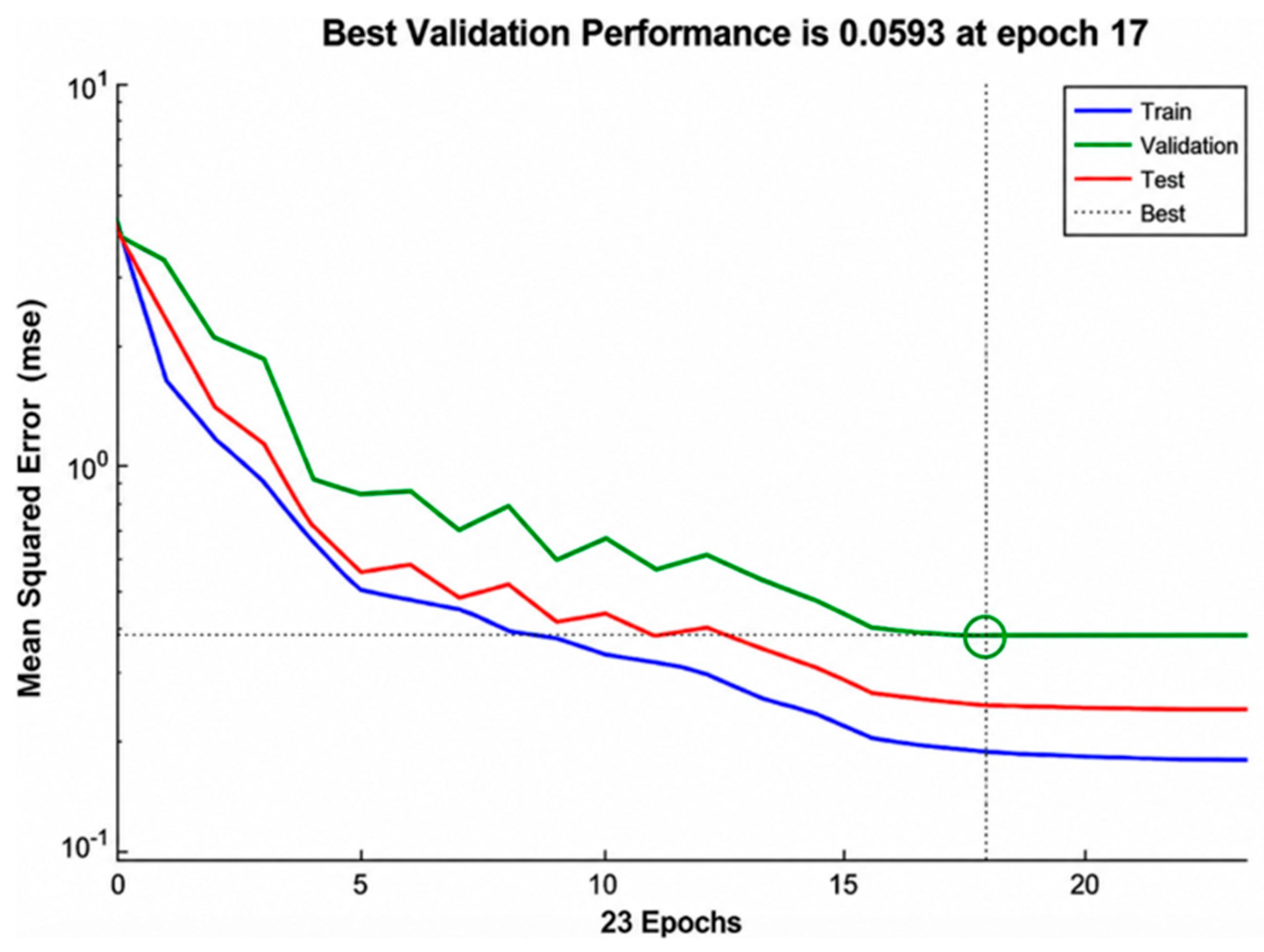
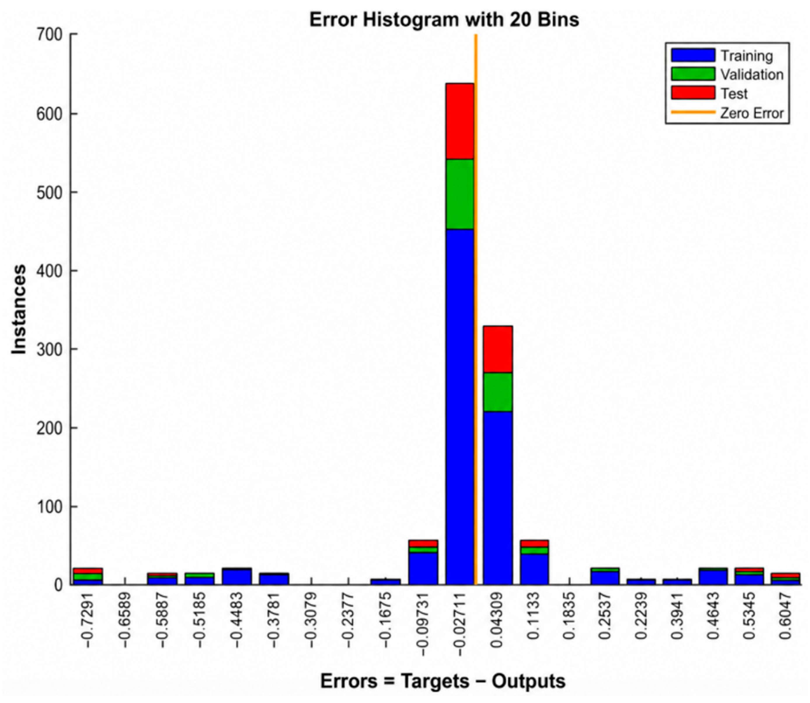
Figure 14 displays the training, validation, and testing MSE curves of the LM-trained ANN for the enlarged high-impedance fault dataset with fault resistance values of 0.01 Ω, 10 Ω, and 50 Ω. Epoch 17 achieves the highest validation performance of 0.0593. The majority of prediction errors are centered at zero, as seen in Figure 15, corresponding to the error histogram. These findings are consistent with continuous learning, adequate generalization, and adequate prediction accuracy in various fault resistance scenarios.

4.3. Fault Location Detection in HVAC System

The proposed ANN-based model for HVAC transmission system fault location detection performance is demonstrated in this section. The trained ANN model locates the fault along the AC transmission line in kilometers using three-phase voltage and current measurements as input features. The following findings confirm the proposed method’s suitability for real-world protection and monitoring applications by showing their efficiency and accuracy in locating different fault types across several fault locations.

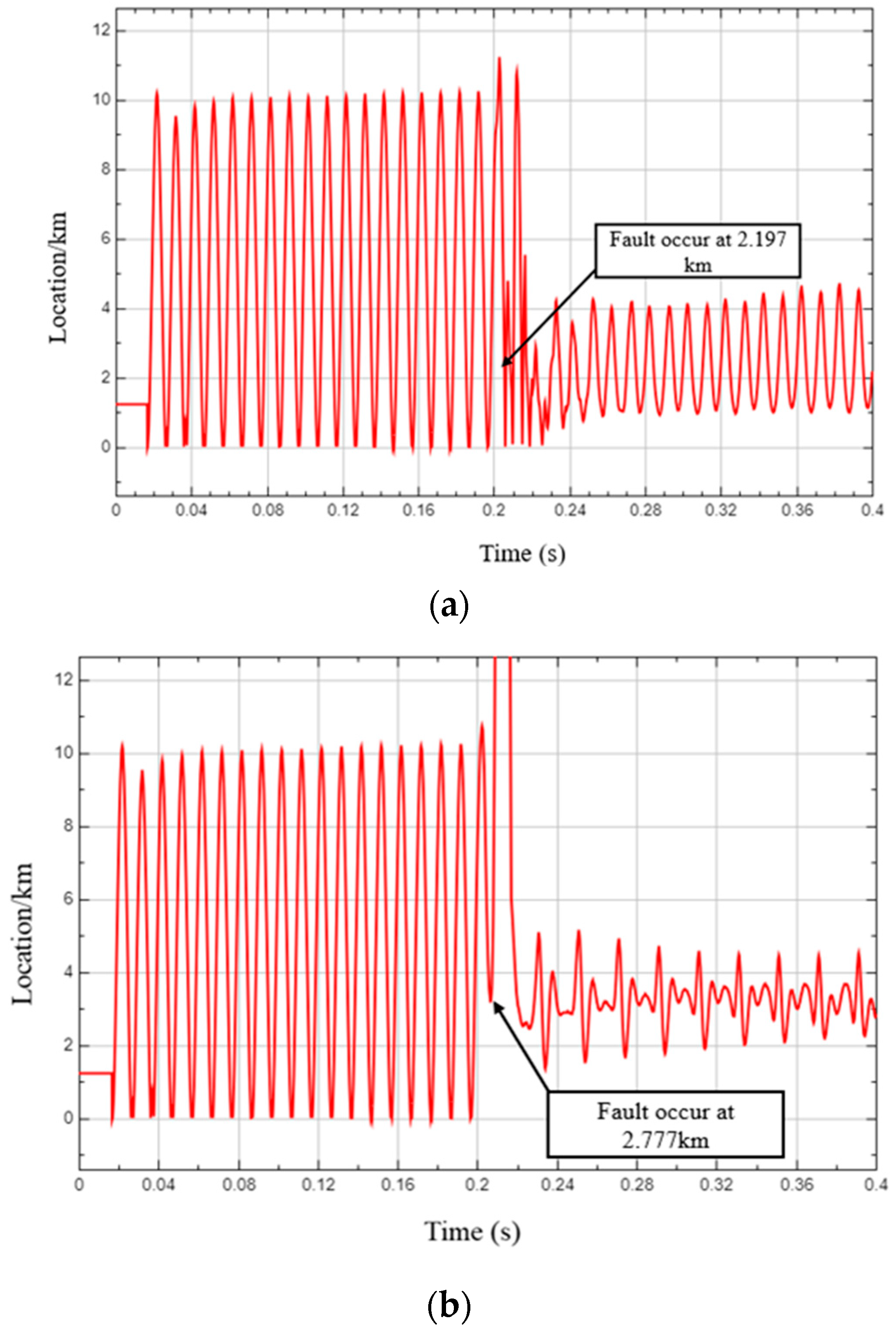
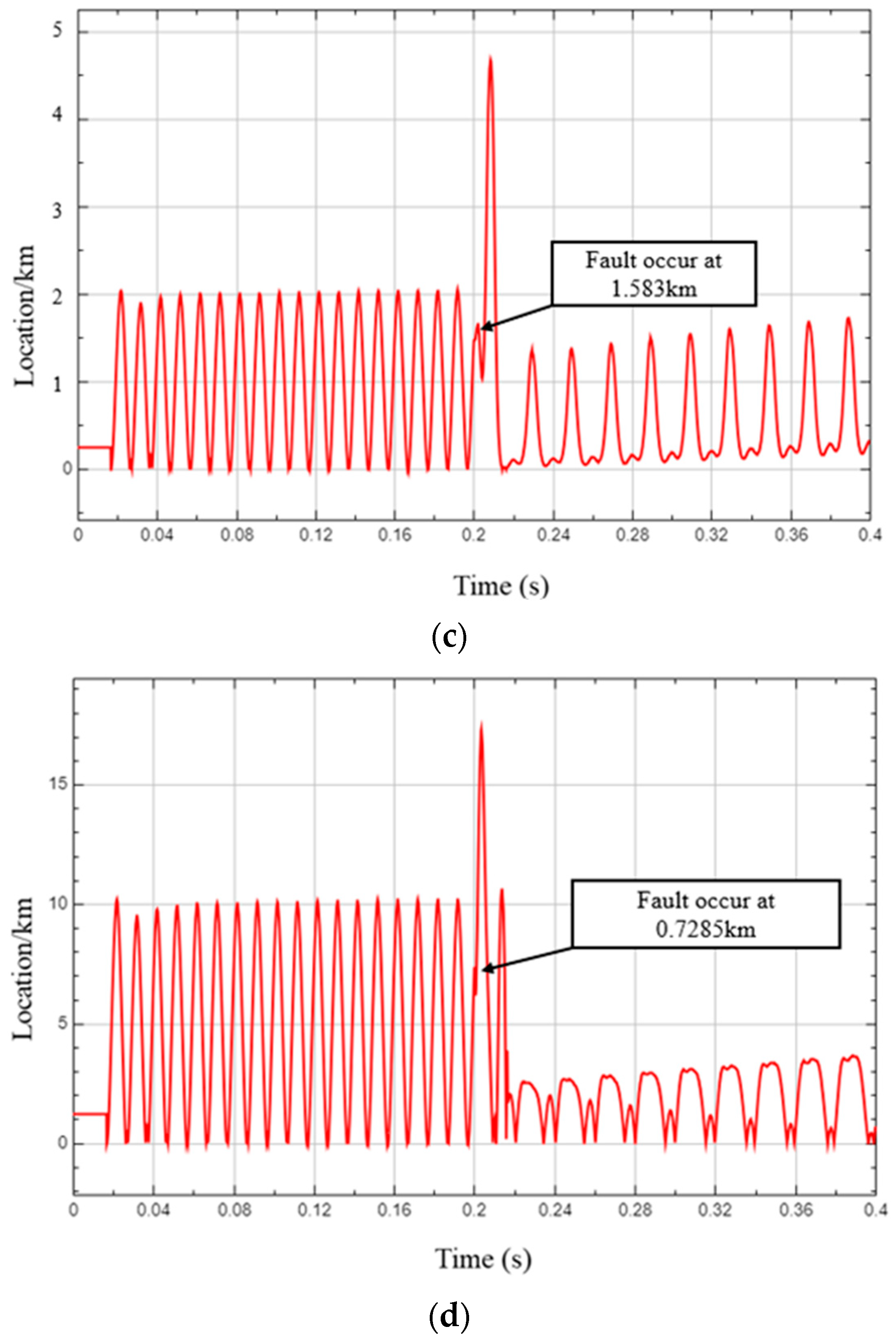
Plotting the predicted fault position in kilometers against the start time, Figure 16 shows the fault start time performance of the proposed ANN-based model for various phase fault conditions along the HVAC transmission line. The location detection for a single line to ground CG fault is shown in Figure 16a, which shows a clear transition at fault inception and rapid convergence to the accurate fault location. The results for an AC_G fault are shown in Figure 16b, which confirms precise and stable localization despite the presence of several phases and ground. The fault location estimation for an AC line-to-line fault is shown in Figure 16c, illustrating the model’s accuracy in locating phase-to-phase faults following brief disruptions. The response for a three-phase to ground ABC_G fault is depicted in Figure 16d, where the ANN reliably converges to the right location with minimal variation. The findings confirm the robustness and efficacy of the proposed method in precisely identifying and localizing various phase fault states on a per-kilometer basis under different fault scenarios.

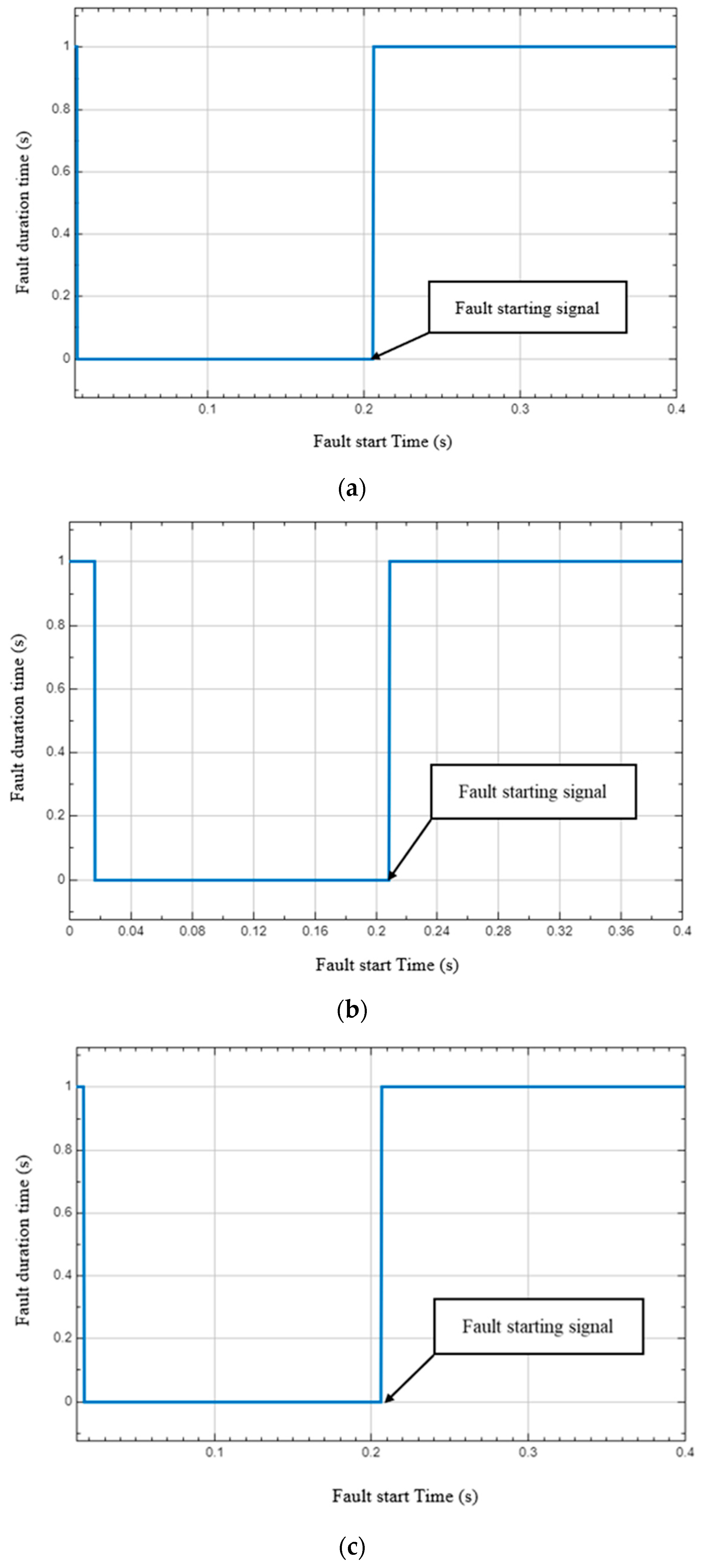
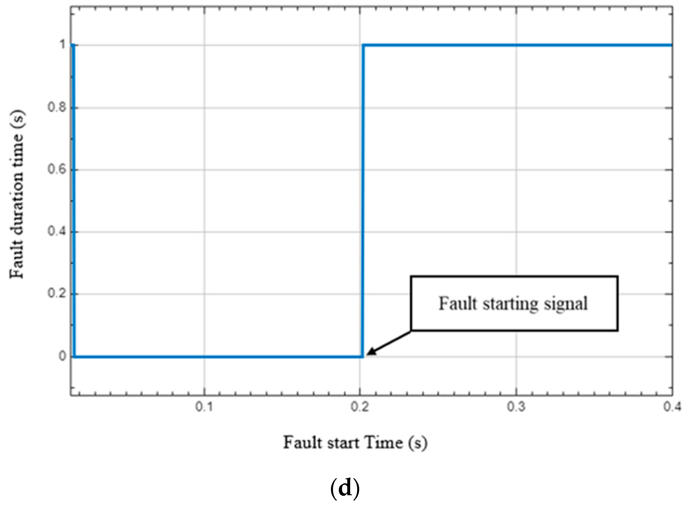
The Fault Location Detection Signals generated by the proposed ANN-based system for different HVAC transmission system fault types are shown in Figure 17. Each inset shows a binary fault detection signal, where the exact fault start instant is shown by a transition from 0 to 1. The detection signal for a single line to ground CG fault is displayed in Figure 17a, which makes the fault’s starting time readily apparent. The response for an AC_G fault is shown in Figure 17b, which shows precise and reliable fault initiation identification even when several phases and ground are present. The fault detection signal for an AC line-to-line fault is shown in Figure 17c, illustrating the ANN’s capacity to accurately determine the fault initiation time under phase-to-phase fault conditions. The detection signal for a three-phase to ground ABC_G fault is shown in Figure 17d, where the abrupt step change accurately indicates the fault occurrence. All of these findings confirm the proposed method’s efficacy in consistently identifying fault initiation across various fault types, which is crucial for precise fault location estimation and ensuing protective measures.

The above findings show that the system is capable of accurately identifying and locating the faulty signals.

Table 12. Performance results of ANN-based fault location detection and classification.

SL. No.	Fault Type	Fault Location in km	Fault Duration	ANN-Based Fault Classification Output
				A	B	C	G
1	A_G	3.929	0.0099	0	0	0	1
2	B_G	2.832	0.1947	0	0	1	0
3	C_G	2.197	0.1937	0	0	1	1
4	AC_G	2.777	0.1911	0	1	0	1
5	AB_G	7.777	0.1862	0	1	0	0
6	BC_G	1.166	0.1981	0	1	1	0
7	AB	0.1989	0.1983	1	0	0	1
8	BC	0.9817	0.1985	1	0	1	1
9	AC	1.583	0.1935	1	0	1	0
10	ABC	0.7285	0.1982	0	1	1	1
11	ABC_G	0.7445	0.1979	1	0	0	0

summarizes typical findings from the ANN-based fault detection, classification, and location modules.

4.4. Critical Clearing Time Based on Threshold Fault Stability Analysis

An important stability measurement in HVAC transmission systems is CCT, which defines how long a fault can last before the system shifts from a stable to an unstable operating condition. Precise evaluation of CCT makes it feasible to differentiate between critical and normal fault conditions, ensuring that preventative measures start within stability thresholds. By integrating fault type with transient stability behavior, CCT analysis improves system reliability and enables HVAC networks to avoid cascading failures by enabling timely protection decisions.

Table 13. Difference between normal fault condition and CCT (calculated).

Case	Fault Type	${\mathbf{T}}_{\mathbf{f}\mathbf{d}}$	${\mathbf{F}}_{\mathbf{s}\mathbf{t}}$	CCT (Calculated)	Location
1	AG	0.4	0.3901	0.0099	3.929
2	ABG	0.4	0.2139	0.1862	7.777
3	ABC	0.4	0.2018	0.1982	0.7285

represents differences between a few cases of normal fault conditions and CCT (calculated).

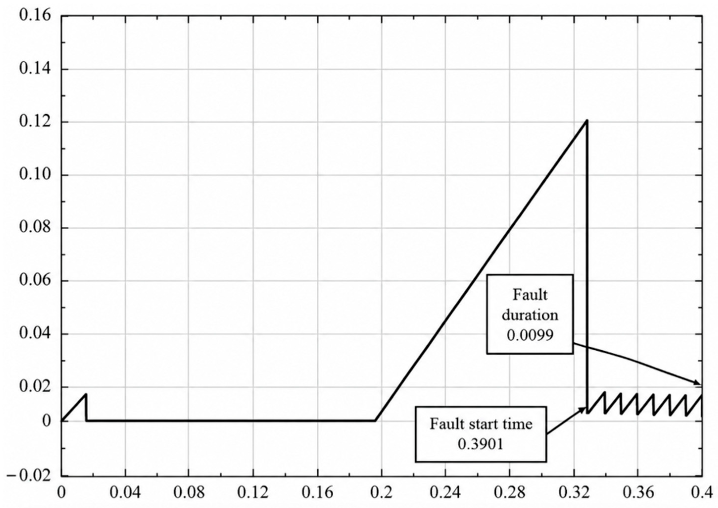
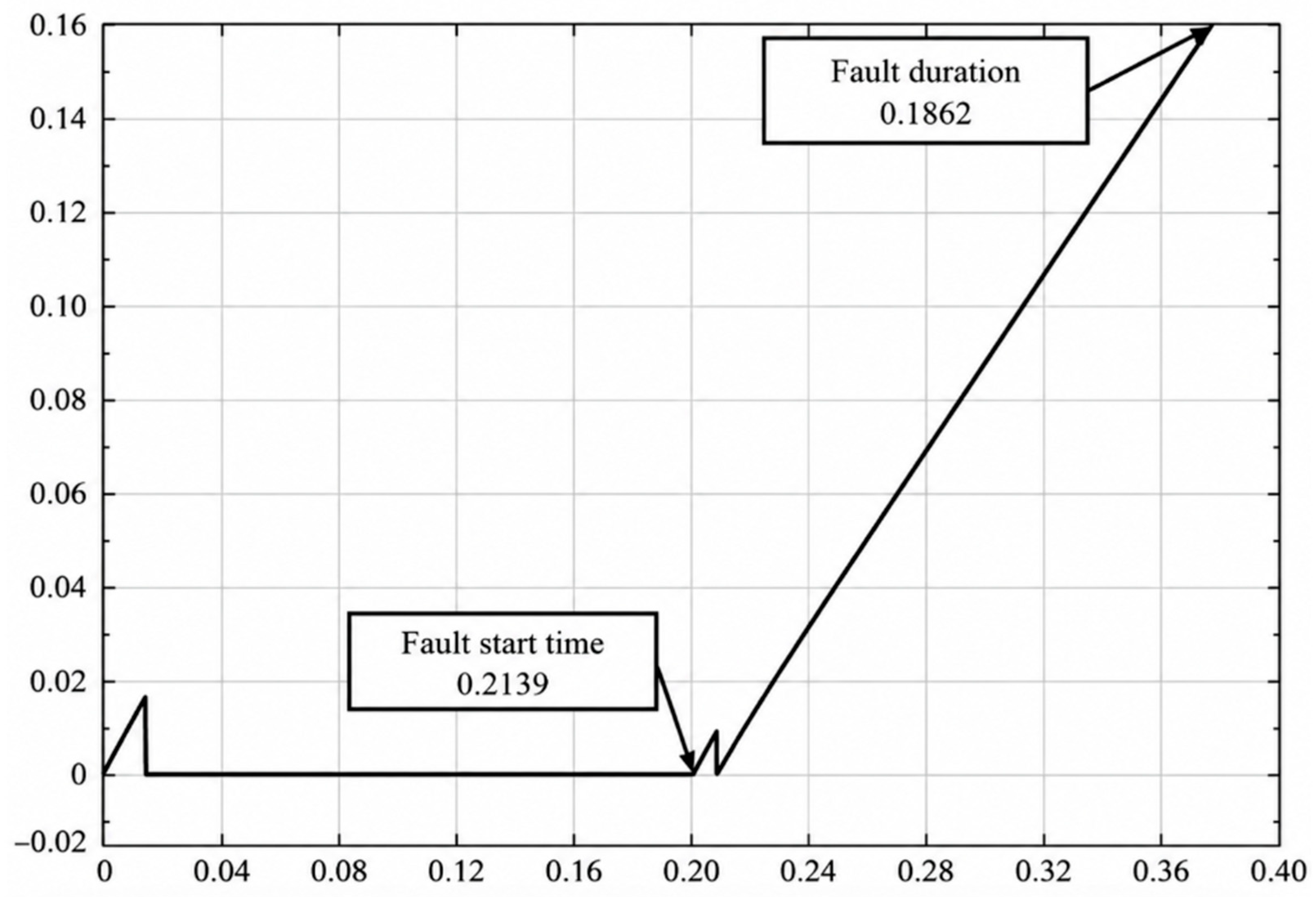
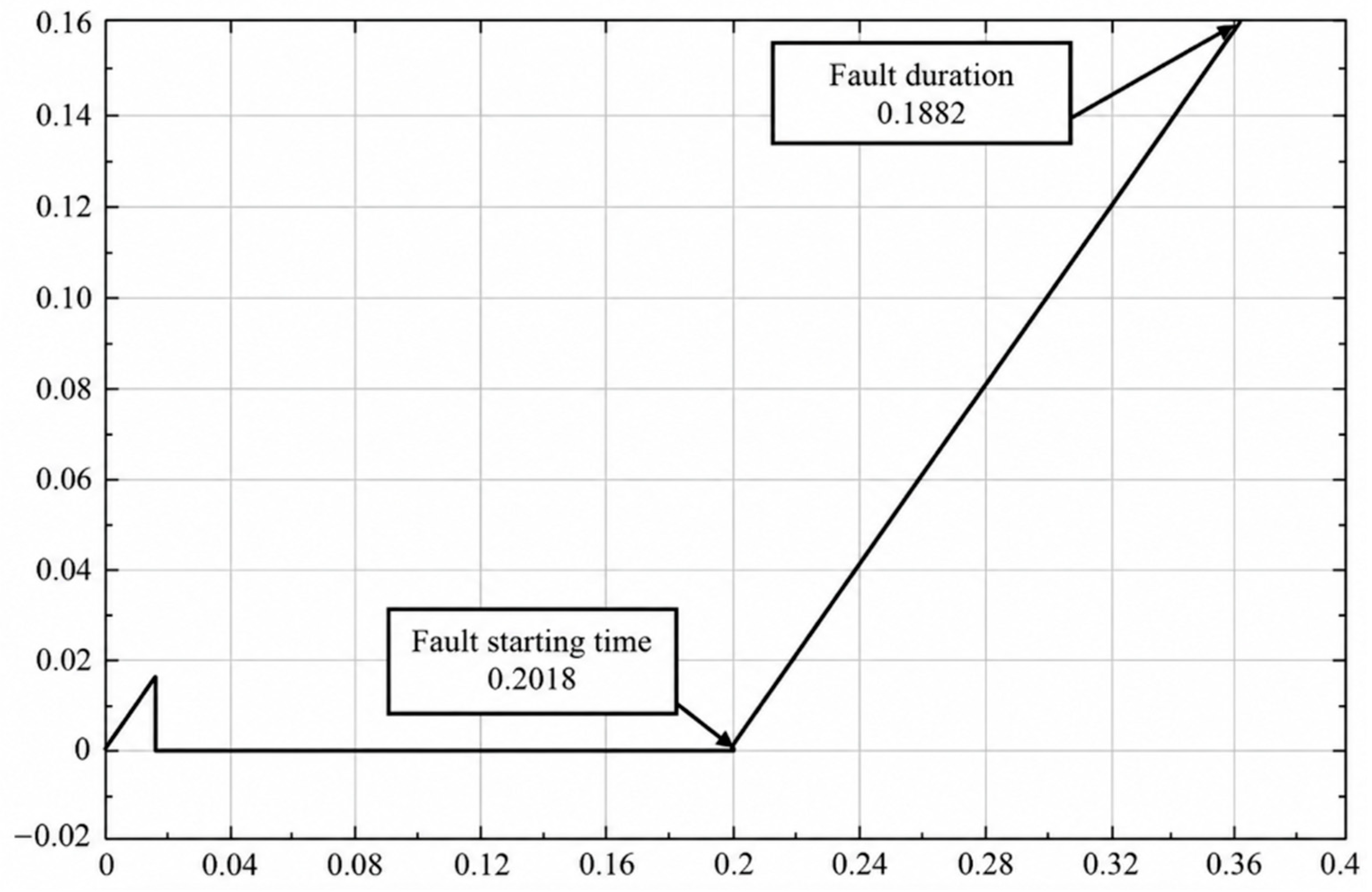
In addition, CCT results in Figure 18, Figure 19 and Figure 20 and Table 13 clearly illustrate how the proposed method utilizes a time threshold parameter to illustrate between normal (non-critical) and stability-critical conditions. The total fault duration ‘T_fd’ is known as 0.4 s, the fault starting time ‘F_st’ is extracted from the simulated fault signal, and the stability margin is calculated using Equation (1). CCT indicates that the system reaches its stability limit almost immediately after the fault occurs, in case-1 (AG, CCT = 0.0099 at 3.929 km), which indicates that the same fault duration would be classified as critical and must be cleared within a very short period of time. For case-2 (ABG, CCT = 0.1862 at 7.777 km) and case-3 (ABC, CCT = 0.1982 at 0.7285 km), which is consistent with typical or non-critical behavior for the clearing time under consideration. Along with identifying the type and location of faults, the proposed structure provides a quantitative stability awareness that decision faults are identified as normal when the observed clearing takes place within the computed CCT margin and critical when the fault persistence surpasses this threshold. This enables protection actions to be scheduled based on stability limits rather than just fault detection.

4.5. Feature Ablation Study of the Proposed LM-Trained ANN Framework

To quantitatively evaluate the contribution of the selected electrical input features to the prediction performance, a feature ablation study was conducted using the same LM-trained ANN architecture, as shown in

Table 14. Feature ablation analysis of the proposed unified framework.

Features Configuration	Input Features	MSE	R
Voltage feature	Va, Vb, Vc	0.1016	0.7708
Current feature	Ia, Ib, Ic	0.0668	0.8545
Without zero-sequence components	Va, Vb, Vc, Ia, Ib, Ic	0.0307	0.9359
Proposed framework	Va, Vb, Vc, Ia, Ib, Ic, V0, I0	0.0401	0.9139

, which consists of a hidden layer size (10 neurons), data partitioning strategy (training 70%, validation 15%, and testing 15%), and Levenberg–Marquardt optimization algorithm. Four input feature configurations were investigated: (i) the complete feature set comprising three-phase voltages (V_a, V_b, V_c), three-phase currents (I_a, I_b, I_c), and zero-sequence components (V₀, I₀), (ii) the exclusion of zero-sequence components, (iii) voltage-only inputs, and (iv) current-only inputs. All experiments were performed using the same 252-sample dataset to ensure a fair and consistent comparison.

The ablation results demonstrate that using only voltage and current measurements significantly degrades the prediction capability of the proposed LM-trained ANN framework, confirming that both feature groups are essential for reliable fault classification and fault location estimation. Although removing the zero-sequence components slightly enhanced numerical performance for the simulation dataset under consideration, the proposed framework retains V₀ and I₀ because they offer useful physical information for ground-fault characterization and enable a unified electrical feature representation applicable to both ground and non-ground fault conditions. The complete eight-feature configuration was retained in the proposed framework to provide an informative and comprehensive electrical feature representation for unified fault classification, fault location estimation, fault timing extraction, and CCT-based stability assessment.

4.6. Comparison with Previous Research Works

The performance of the proposed LM-optimized ANN model is compared with traditional as well as modern HVAC fault detection methods to evaluate it further. Traveling wave and impedance-based techniques rely on precise line parameters and high-frequency measurements, which makes them susceptible to noise, fault resistance, and signal distortion. They also need strict time synchronization and high sampling rates, which limit their applicability in real-time. Transients can be captured using signal processing techniques like wavelet or frequency-domain features, but they frequently lack integrated outputs, including fault location, fault duration, or stability indices, and usually require manual feature engineering and threshold measurement.

The accuracy of classification is generally improved compared to recent machine learning techniques such as KNN, DT, SVM, and different types of ML models. Many studies are limited to a subset of fault scenarios and concentrate mainly on classification. The proposed LM-optimized ANN model provides a single solution that simultaneously carries out stability-aware CCT evaluation, fault starting time and duration extraction, multi-class fault classification, and per km fault location detection. This functional accuracy, along with LM quick convergence and low error, makes the technique more appropriate for intelligent real-time monitoring and protection for modern HVAC networks. A comparative analysis includes traditional and current intelligent fault detection methods utilized in HVAC transmission systems to further demonstrate the efficacy of the proposed technique, as shown in

Table 15. Comparative performance analysis of fault detection techniques in HVAC transmission systems.

Method	Types of Faults	Location	Timing	CCT	Real-Time Suitability	Unified Protection Framework
Impedance-based [18]	limited	-	no	no	medium	no
Traveling wave [18]	Short circuit	partial	yes	no	low	no
Wavelet based [12,20]	limited	partial	partial	no	medium	no
(KNN/SVM) [12,15,16]	partial	limited	no	no	low	no
CNN-based ML [13]	Most types of faults	limited	partial	no	medium	no
RNN OR LSTM-based ML [14]	Most types of faults	limited	yes	no	medium	no
CNN, LSTM/GRU [22]	Most types of faults	partial	partial	no	medium	no
GRU [23]	partial	-	-	no	low	no
Proposed model	All types of faults	High	yes	yes	High	yes

Note: Limited indicates that the location accuracy is typically less than 80% or that the method supports only a limited subset of fault cases. Partial indicates that the method provides incomplete information, such as approximate fault location detection or limited temporal analysis without full fault characterization. High indicates location accuracy typically greater than 95%. In terms of real-time suitability, high corresponds to response times below 10 ms, medium corresponds to 10–50 ms, and low corresponds to response times greater than 50 ms due to higher computational or synchronization requirements.

. The comparison highlights the practical benefits of the proposed model by focusing on important functional features such as fault type coverage, fault location capabilities, timing information, CCT consideration, and real-time adaptability.

5. Conclusions

An LM-trained ANN-based model for HVAC transmission system fault detection, classification, location estimation, and stability assessment was presented in this study. The HVAC simulation was developed in MATLAB Simulink to systematically simulate twelve different fault types, including single-line, double-line, three-phase, and ground-controlled conditions at different transmission line locations. With a regression coefficient of R = 0.9882 and a mean squared error of MSE = 0.1386, the numerical results demonstrate that the proposed ANN model achieves superior detection reliability, confirming accurate nonlinear learning of fault dynamics.

The major findings of the proposed method indicate that the ANN-based fault classification approach consistently and accurately identifies phase involvement and ground participation across all investigated fault scenarios. The developed fault location module effectively estimates the fault position along the transmission line on a per-kilometer basis, demonstrating fast convergence and high accuracy for different fault conditions. The extracted fault duration and starting time enable the numerical evaluation of system stability using CCT analysis. The computed CCT values allow clear differentiation between stability-critical faults, such as the AG fault with CCT = 0.0099 s at 3.929 km, and normal fault conditions, such as ABG and ABC faults with CCT ≈ 0.19 s. These results demonstrate that the proposed framework provides a comprehensive solution by simultaneously delivering fault type identification, precise fault location detection, timing information, and CCT-based stability assessment within a single model. The fast convergence characteristics of the Levenberg–Marquardt optimization algorithm ensure efficient ANN training, making the proposed technique suitable for intelligent real-time protection applications in modern HVAC transmission networks. The comparative optimizer analysis further confirmed that LM outperformed BR and SCG by achieving fewer convergence epochs, lower prediction error, and higher regression accuracy. In addition to the baseline 0.01 Ω case, the proposed framework was further validated under high-impedance fault conditions by incorporating fault resistance values of 10 Ω and 50 Ω. The obtained results confirm the robustness of the LM-trained ANN by showing that it maintains satisfactory prediction capability under varying fault resistance conditions, supporting its suitability for practical HVAC transmission line protection.

To evaluate dependability and enhance model generalization, future research will further expand the simulation-generated dataset through additional fault locations, loading conditions, and noisy measurement scenarios. To improve generalization under intricate nonlinear transients, the model will be expanded utilizing hybrid machine learning architectures (wavelet or feature-assisted ML and ensemble learning). To ensure optimal substation level protection coverage, the method will be modified to include busbar fault detection and classification in addition to transmission line problems. In addition, integration with real-time hardware in the loop (HIL) systems and PMU-based wide area measurements are planned to assess latency limits and practical implementation viability. Developing the structure of multi-terminal networks and hybrid HVAC/DC systems, as well as adding deeper designs for scaling to bigger grids, is a potential field for more research.

References

1. Xing, J.; Han, C.; Tian, J.; Wu, H.; Lu, T. Influence of Ion Flow Field on the Design of Hybrid HVAC and HVDC Transmission Lines with Different Configurations. Energies 2025, 18, 3657. [Google Scholar] [CrossRef] [Scilit]
2. Fayazi, M.; Saffarian, A.; Joorabian, M.; Monadi, M. Analysis of induced components in hybrid HVAC/HVDC transmission lines on the same tower for various fault conditions. Electr. Power Syst. Res. 2024, 226, 109884. [Google Scholar] [CrossRef] [Scilit]
3. Borghett, F.; Giovanni Colombo, C.; Longo, M.; Mazzoncini, R.; Somaschini, C. Development of a new urban line with innovative trams. In Proceedings of the Urban and Maritime Transport 2021; WIT Press: Billerica, MA, USA, 2021; pp. 167–178. [Google Scholar] [CrossRef] [Scilit]
4. Mishra, D.P.; Ray, P. Fault detection, location and classification of a transmission line. Neural Comput. Appl. 2018, 30, 1377–1424. [Google Scholar] [CrossRef] [Scilit]
5. Liu, Y.; Wu, J.; Zhang, J.; Leung, M.-F. Graph-Regularized Orthogonal Non-Negative Matrix Factorization with Itakura–Saito (IS) Divergence for Fault Detection. Mathematics 2025, 13, 2343. [Google Scholar] [CrossRef] [Scilit]
6. Martino, A.D.; Prasad, G.S.; Foiadelli, F.; Longo, M. Energy Demand Model of Battery E-Buses for LPT: Implementation, Validation and Scheduling Optimization. IEEE Access 2023, 11, 52185–52198. [Google Scholar] [CrossRef] [Scilit]
7. Bindi, M.; Piccirilli, M.C.; Luchetta, A.; Grasso, F. A Comprehensive Review of Fault Diagnosis and Prognosis Techniques in High Voltage and Medium Voltage Electrical Power Lines. Energies 2023, 16, 7317. [Google Scholar] [CrossRef] [Scilit]
8. Adami, J.F.; Silveira, P.M.; Martinez, M.; Perez, R.C.; Dallbello, A.C. New Approach to Improve High-Voltage Transmission Line Reliability. IEEE Trans. Power Deliv. 2009, 24, 1515–1520. [Google Scholar] [CrossRef] [Scilit]
9. Hazari, M.d.R.; Abu Talha, M.; Ahmad, S.; Jahan, E.; Hossain, C.A.; Abdul Mannan, M. Performance Analysis of Hybrid Power System with Wind Farms and Conventional Generators Under Fault Conditions. In Proceedings of the 2025 10th International Conference on Business and Industrial Research (ICBIR); IEEE: Bangkok, Thailand, 2025; pp. 381–386. [Google Scholar] [CrossRef] [Scilit]
10. Yadav, A.; Dash, Y. An Overview of Transmission Line Protection by Artificial Neural Network: Fault Detection, Fault Classification, Fault Location, and Fault Direction Discrimination. Adv. Artif. Neural Syst. 2014, 2014, 230382. [Google Scholar] [CrossRef] [Scilit]
11. Ahmad, S.; Hasan, S.M.d.N.; Hossain, M.d.S.; Uddin, R.; Ahmed, T.; Mustayen, A.G.M.B.; Hazari, M.d.R.; Hassan, M.; Parvez, M.d.S.; Saha, A. A Review of Hybrid Renewable and Sustainable Power Supply System: Unit Sizing, Optimization, Control, and Management. Energies 2024, 17, 6027. [Google Scholar] [CrossRef] [Scilit]
12. Naik, S.; Koley, E. Fault Detection and Classification scheme using KNN for AC/HVDC Transmission Lines. In Proceedings of the 2019 International Conference on Communication and Electronics Systems (ICCES); IEEE: Coimbatore, India, 2019; pp. 1131–1135. [Google Scholar] [CrossRef] [Scilit]
13. Johnson, J.M.; Yadav, A. Fault Detection and Classification Technique for HVDC Transmission Lines Using KNN. In Information and Communication Technology for Sustainable Development; Mishra, D.K., Nayak, M.K., Joshi, A., Eds.; Lecture Notes in Networks and Systems; Springer: Singapore, 2018; Volume 10, pp. 245–253. [Google Scholar] [CrossRef] [Scilit]
14. Jawad, R.S.; Abid, H. HVDC Fault Detection and Classification with Artificial Neural Network Based on ACO-DWT Method. Energies 2023, 16, 1064. [Google Scholar] [CrossRef] [Scilit]
15. Özüpak, Y. Machine learning-based fault detection in transmission lines: A comparative study with random search optimization. Bull. Pol. Acad. Sci. Tech. Sci. 2025, 73, e153229. [Google Scholar] [CrossRef] [Scilit]
16. Ahmed, S.I.; Rahman, M.F.; Kundu, S.; Chowdhury, R.M.; Hussain, A.O.; Ferdoushi, M. Deep Neural Network Based Fault Classification and Location Detection in Power Transmission Line. In Proceedings of the 2022 12th International Conference on Electrical and Computer Engineering (ICECE); IEEE: Dhaka, Bangladesh, 2022; pp. 252–255. [Google Scholar] [CrossRef] [Scilit]
17. Minh, N.Q.; Khiem, N.T.; Giang, V.H. Fault classification and localization in power transmission line based on machine learning and combined CNN-LSTM models. Energy Rep. 2024, 12, 5610–5622. [Google Scholar] [CrossRef] [Scilit]
18. Tiferes, R.R.; Manassero, G., Jr.; Lacerda, V.A.; Gomis-Bellmunt, O. Comparative evaluation of conventional and advanced HVAC line protection algorithms: A case study. IET Conf. Proc. 2025, 2025, 290–296. [Google Scholar] [CrossRef] [Scilit]
19. Shakiba, F.M.; Shojaee, M.; Azizi, S.M.; Zhou, M. Real-Time Sensing and Fault Diagnosis for Transmission Lines. Int. J. Netw. Dyn. Intell. 2022, 1, 36–47. [Google Scholar] [CrossRef] [Scilit]
20. Saleem, U.; Arshad, U.; Masood, B.; Gul, T.; Khan, W.A.; Ellahi, M. Faults detection and classification of HVDC transmission lines of using discrete wavelet transform. In Proceedings of the 2018 International Conference on Engineering and Emerging Technologies (ICEET); IEEE: Lahore, Pakistan, 2018; pp. 1–6. [Google Scholar] [CrossRef] [Scilit]
21. Yoon, D.-H.; Yoon, J. Development of a real-time fault detection method for electric power system via transformer-based deep learning model. Int. J. Electr. Power Energy Syst. 2024, 159, 110069. [Google Scholar] [CrossRef] [Scilit]
22. Kouraichi, M.; Mansouri, M.; Trabelsi, M.; M’Halla, A.; Abdel-Khalik, A.S.; Sakly, A. Deep Learning for Fault Diagnosis in Power Transmission Lines: Current Trends, Limitations, and Future Directions. IEEE Access 2025, 13, 192105–192142. [Google Scholar] [CrossRef] [Scilit]
23. Hu, H.; Lu, H.; Shi, R.; Fan, X.; Deng, Z. A novel fault diagnosis method for key transmission sections based on Nadam-optimized GRU neural network. Electr. Power Syst. Res. 2024, 233, 110522. [Google Scholar] [CrossRef] [Scilit]
24. Kaur, H.; Kaur, M. Fault Classification in a Transmission Line Using Levenberg–Marquardt Algorithm Based Artificial Neural Network. In Data Communication and Networks; Jain, L.C., Tsihrintzis, G.A., Balas, V.E., Sharma, D.K., Eds.; Advances in Intelligent Systems and Computing; Springer: Singapore, 2020; Volume 1049, pp. 119–135. [Google Scholar] [CrossRef] [Scilit]
25. Edalatifar, M.; Ghalambaz, M.; Tavakoli, M.B.; Setoudeh, F. New loss functions to improve deep learning estimation of heat transfer. Neural Comput. Appl. 2022, 34, 15889–15906. [Google Scholar] [CrossRef] [Scilit]
Figure 1. Classification of the different types of faults.
Energies 19 03405 g001
Figure 2. Basic block diagram of optimized machine learning-based fault detection.
Energies 19 03405 g002
Figure 3. HVAC transmission line model.
Energies 19 03405 g003
Figure 4. Correlation matrix.
Energies 19 03405 g004
Figure 5. Sensitive analysis.
Energies 19 03405 g005
Figure 6. Levenberg–Marquardt optimization-based ANN training flowchart for HVAC fault detection.
Energies 19 03405 g006
Figure 7. ANN-Based Neural Network Structure.
Energies 19 03405 g007
Figure 8. Unified intelligent protection framework.
Energies 19 03405 g008
Figure 9. Training performance curve optimized with Levenberg–Marquardt for fault classification and detection.
Energies 19 03405 g009
Figure 10. Classification of fault detection in HVAC (a) Single phase to ground fault and (b) Single phase to ground fault current condition.
Energies 19 03405 g010
Figure 11. Classification of fault detection in HVAC (a) double line to ground fault and (b) double line to ground fault current condition.
Energies 19 03405 g011
Figure 12. Classification of fault detection in HVAC (a) line-to-line fault and (b) line-to-line fault current condition.
Energies 19 03405 g012
Figure 13. Classification of fault detection in HVAC (a) three-phase to ground fault and (b) three-phase to ground fault current condition.
Energies 19 03405 g013
Figure 14. Training performance curve of the LM-trained ANN under high-impedance fault conditions.
Energies 19 03405 g014
Figure 15. Error histogram of the LM-trained ANN under varying fault resistance conditions.
Energies 19 03405 g015
Figure 16. Fault start time as per distance (km) for different phase fault conditions (a) Fault location detection in CG, (b) Fault location detection in AC_G, (c) Fault location detection in AC, and (d) Fault location detection in ABC_G.
Energies 19 03405 g016aEnergies 19 03405 g016b
Figure 17. Different types of Fault Location Detection Signals (a) Fault Location Detection Signal for CG, (b) Fault Location Detection Signal for AC_G, (c) Fault Location Detection Signal for AC, and (d) Fault Location Detection Signal for ABC_G.
Energies 19 03405 g017aEnergies 19 03405 g017b
Figure 18. AG fault as per CCT calculation.
Energies 19 03405 g018
Figure 19. ABG fault as per CCT calculation.
Energies 19 03405 g019
Figure 20. ABC fault as per CCT calculation.
Energies 19 03405 g020