Risk-Anchored Order-Preserving Scenario-Chain Construction for Renewable Energy Base Planning

Abstract

Large renewable energy bases are increasingly planned under delivery-hour targets, corridor-capacity constraints, and high shares of wind and photovoltaic generation. Chronological planning samples used in expansion and adequacy studies therefore need to retain not only average renewable-load patterns but also low-probability days with high residual balancing demand, large ramps, curtailment pressure, and sustained renewable scarcity. This paper proposes a risk-anchored order-preserving scenario-chain construction method for renewable energy base planning. The proposed method transforms aligned hourly load, wind, photovoltaic, delivery-demand, and loss-adjusted demand trajectories into distinct operational stress indicators, normalizes them into a joint extreme score, anchors the highest-risk natural days together with their adjacent transition days, and applies clustering only to the remaining regular days. Observed medoid days are then inserted back into chronological order to form a compact scenario chain with explicit weights and adjacency information. A representative 8760 h renewable-base case with 4000 MW wind, 5500 MW photovoltaic, 5400 MW coal support, 1200 MWh storage-energy capacity, a 7600 MW delivery corridor, and a 5600 h delivery target is used to run weight-sensitivity tests and same-budget comparisons against monthly typical days, k-means, k-medoids, hierarchical clustering, Carpe Diem, and seasonal time-series aggregation baselines. Under the equal-weight base case, the proposed chain gives an active-metric mean capture ratio of 1.0660, compared with 0.8377 for monthly typical days. Across four non-equal priority-weight vectors, the active-metric mean remains between 1.0041 and 1.0662. Under the same 151-day budget, conventional k-means, k-medoids, hierarchical clustering, Carpe Diem, and seasonal time-series aggregation baselines obtain active-metric means of 0.8643, 0.9025, 0.8732, 0.9239, and 0.9189, respectively. The results indicate that chronological risk anchoring provides a compact yet physically interpretable sampling layer for planning models that must balance renewable utilization, delivery reliability, and storage adequacy.

1. Introduction

1.1. Motivation

Large wind-photovoltaic bases connected through high-capacity transmission corridors are no longer planned as isolated generation portfolios. Their planning problem couples resource variability, delivery commitments, thermal support, storage sizing, corridor utilization, and risk tolerance over thousands of hourly operating states. A full 8760 h representation remains attractive because it preserves sequence-dependent phenomena, but full-year chronological models rapidly become expensive when embedded in capacity expansion, unit commitment, network reinforcement, or storage planning formulations.

Temporal aggregation is therefore widely used, yet its practical value depends on the ability to preserve the events that actually drive planning decisions. Average representative days may reproduce annual energy shares, but a renewable base is often stressed by a small set of days with simultaneous renewable shortage, steep net-load variation, curtailment exposure, or prolonged low-output intervals. If these events are smoothed out before the planning optimization is solved, the resulting capacity mix can be biased toward underestimating flexibility, storage duration, and reserve requirements.

The central premise of this study is that scenario-chain construction should be risk-aware before it is compact. Rather than clustering all days and hoping that rare events survive the compression, the proposed method first identifies high-stress natural days, retains their neighboring transition days, and only then applies representative-day selection to regular days. This strategy maintains a chronological bridge between extreme conditions and normal operation while preserving the computational advantages of a reduced temporal sample.

1.2. Related Work

Representative-period selection has become a central mechanism for reducing chronological planning models with high renewable penetration. Poncelet et al. developed a representative-day framework for generation expansion planning and showed that the selected days can change the implications of intermittent renewable integration [1]. Liu et al. proposed hierarchical clustering to identify representative operating periods for capacity-expansion modeling, improving tractability while retaining diverse operating regimes [2]. Sun et al. moved the criterion closer to investment decisions by proposing a cost-oriented, data-driven representative-day selection method [3]. Garcia-Cerezo et al. then enhanced representative time periods for transmission expansion planning, indicating that the temporal sample must be tailored to network decisions rather than selected only by statistical similarity [4]. A later priority chronological clustering method further showed that long-term dynamics require a temporal representation that preserves sequence-dependent behavior, not only representative states [5].

A second stream focuses on uncertainty scenario generation and scenario reduction. Zhuo et al. incorporated massive scenarios into transmission expansion planning with high renewable penetration, demonstrating that planning decisions become sensitive to tail and correlation structures when renewable variability is represented explicitly [6]. Li et al. generated long-term wind and photovoltaic scenarios with an attention-based conditional generative adversarial network, showing that data-driven scenario generation can capture both seasonal dependence and intraday renewable-output structure [7]. Zhan et al. proposed a fast solution method for stochastic transmission expansion planning, showing that computational tractability and uncertainty fidelity must be addressed together [8]. Wang et al. formulated scenario reduction with submodular optimization, providing a principled way to retain informative scenarios under a limited sample budget [9]. Hu and Li proposed a clustering approach for scenario reduction in multi-stochastic-variable programming, emphasizing the role of multivariate dependence in reduced scenario sets [10]. These studies are methodologically close to the present work, but most of them either generate scenarios or reduce scenarios without first protecting physically interpretable extreme days and their adjacent transitions.

Planning studies under renewable uncertainty also clarify which operating events should be preserved by temporal compression. Li et al. considered coordinated transmission and generation expansion with ramping requirements and construction periods, showing that ramping constraints can materially affect expansion decisions [11]. Jabr developed robust transmission expansion planning under uncertain renewable generation and loads, highlighting the need to protect worst-case renewable-load combinations [12]. Park et al. modeled dependent load and wind forecasts in stochastic transmission planning, illustrating why chronological and correlation information cannot be ignored [13]. Qiu et al. introduced a probabilistic framework for reducing network vulnerability to extreme events [14], and their risk-based multi-stage planning approach connected probabilistic exposure with staged network decisions [15]. Orfanos et al. studied transmission expansion under increasing wind integration, confirming that renewable-rich systems require planning models that explicitly recognize variability-driven network stress [16].

IEEE work on flexibility, storage, and reserve provision provides an additional planning rationale for the proposed risk indicators. Tejada-Arango et al. proposed power-based generation expansion planning for flexibility requirements, which directly links investment adequacy to ramping and operating flexibility [17]. Moreira et al. formulated flexible transmission network planning under uncertainty as a min–max regret problem, demonstrating that robust network decisions depend on adverse temporal realizations [18]. Dvorkin et al. co-planned transmission and merchant energy storage investments, revealing that storage value depends on congestion and chronological price or dispatch patterns [19]. Qin et al. further modeled pipeline energy storage in a non-isothermal multi-energy system, indicating that storage value can be embedded in dynamic network states rather than represented only by static capacity limits [20]. Dehghan and Amjady jointly planned transmission and energy storage expansion in wind-integrated systems, showing that storage and network reinforcement should be coordinated under renewable uncertainty [21]. Canas-Carreton and Carrion examined generation expansion when wind units provide reserve, further linking renewable variability, reserve adequacy, and expansion decisions [22].

Non-IEEE energy-system studies remain useful for positioning the temporal aggregation problem. Denholm and Hand established that high renewable penetration increases the need for storage and grid flexibility [23]. Brown et al. showed that sector coupling and transmission reinforcement can interact strongly in highly renewable systems [24]. Wang et al. demonstrated that dynamic carbon-market signals can reshape multi-stage scheduling in hydrogen integrated energy systems, which reinforces the need for reduced chronologies that preserve policy-sensitive operating states rather than only average renewable profiles [25]. Schill and Zerrahn quantified long-run storage requirements under high renewable shares [26]. Nahmmacher et al. introduced the Carpe Diem representative-day approach for long-term power system modeling [27]. Kotzur et al. compared time-series aggregation methods and later demonstrated the importance of seasonal storage modeling under aggregated time series [28,29]. Teichgraeber and Brandt compared clustering methods for energy-system optimization [30], Hoffmann et al. reviewed time-series aggregation methods [31], Gonzato et al. examined long-term storage under reduced temporal scopes [32], and Moradi-Sepahvand and Tindemans introduced representative days and hours with piecewise linear transitions [33].

Taken together, the above literature indicates three unresolved issues for renewable energy base planning. First, representative-day, scenario-generation, and scenario-reduction methods are increasingly sophisticated, yet many still choose compact samples through global similarity, generative fidelity, or optimization value without explicitly protecting the natural days that jointly exhibit high net load, severe ramping, curtailment pressure, or sustained renewable scarcity. Second, transmission, generation, storage, hydrogen-integrated energy, and carbon-constrained scheduling studies show that adverse temporal realizations can drive planning or operating outcomes, but they rarely provide a transparent preprocessing rule that preserves the adjacent-day context around those realizations. Third, chronological clustering methods recognize sequence dependence, but the integration of risk anchoring, adjacent-day buffering, observed medoid-day selection, and metric-specific capture evaluation remains incomplete. These gaps motivate the risk-anchored order-preserving scenario-chain framework proposed in this paper.

1.3. Contributions and Paper Organization

This paper makes three contributions. First, it defines a multi-indicator extreme score that combines residual balancing requirement, ramping magnitude, curtailment sensitivity after absorbable surplus is considered, and continuous low-output intensity under a unified normalization framework. Second, it proposes an extreme-day anchoring mechanism that keeps high-risk natural days and their adjacent days intact before clustering. Third, it constructs an order-preserving scenario chain that provides hourly indices, weights, and adjacency relations for downstream planning models, while explicitly noting that chronological sorting is a reduced-chain ordering rule rather than a guarantee that all skipped physical days are represented continuously. The remainder of the paper formulates the risk indicators in Section 2, presents the scenario-chain construction method in Section 3, describes the case design in Section 4, discusses numerical results in Section 5, and concludes in Section 6.

2. Problem Formulation and Operational Stress Indicators

2.1. Chronological Input Representation

The proposed construction begins from an hourly chronological state rather than from pre-aggregated days. This choice is important because the same annual renewable energy share can lead to different planning decisions when low-output intervals, ramping events, and delivery peaks occur in different orders. The hourly state vector is defined as

$$X_t=(L_t,W_t,P_t,D_t),t=1,\dots ,T$$

(1)

where $L_t$ is the local or equivalent load, $W_t$ and $P_t$ are wind and photovoltaic availability factors or normalized outputs, and $D_t$ is the scheduled delivery demand. Keeping these variables in the same vector makes every subsequent indicator inherit the same timestamp and avoids a loss of correlation between renewable production and delivery requirement.

At the case-study scale, $X_t$ is also the unit at which data quality is audited. The four entries must be sampled over the same clock hour; otherwise, a shortage caused by low $W_t$ and $P_t$ could be matched with a delivery target $D_t$ from another hour, producing an artificial stress signal. This alignment is especially important for renewable-energy-base planning because export schedules are usually evaluated by hour, while wind and photovoltaic profiles can change substantially within a day.

Mathematically, $X_t$ defines the common domain for all later transformations. Equations (2) and (3) are pointwise mappings from $X_t$ to $G_t^{re}$ and $N_t$, while the ramping and persistence indicators in Section 2.2 use adjacent or trailing values of the same time-indexed sequence. The formulation therefore keeps physical chronology before any reduction is introduced.

For installed wind capacity $P_w$ and photovoltaic capacity $P_p$, the renewable generation potential is

$$G_t^{re}=P_w{W}_t+P_p{P}_t$$

(2)

In the case study, D_t denotes the total equivalent hourly demand imposed on the renewable base after local-load consolidation. If a dataset reports local load and external delivery demand separately, the balance can be written as N_t = D_t^del + L_t − G_t^re; if network losses are represented exogenously, D_t can be replaced by D_t/(1 − λ_t) or by D_t + L_t^loss. This clarification prevents L_t from being ignored while avoiding double counting when the supplied D_t series is already a total equivalent demand trajectory.

$$N_t=D_t-G_t^{re}$$

(3)

Equation (3) is the hinge between the resource trajectory and the planning-risk trajectory. A positive $N_t$ means that the delivery schedule still requires support from dispatchable generation, storage discharge, imports, or demand-side flexibility. A negative $N_t$ means that renewable production exceeds the delivery demand and may create curtailment or storage-charging pressure. To make this sign-dependent interpretation explicit, the net load is decomposed into two nonnegative components:

$$B_t=max\{N_t,0\}$$

(4)

$$U_t=max\{-N_t,0\}$$

(5)

Here, $B_t$ is the residual balancing requirement and $U_t$ is the instantaneous renewable surplus potential. The decomposition does not replace $N_t$; instead, it clarifies why the later indicator stack needs both adequacy-oriented and curtailment-oriented terms. In this way, the method links resource adequacy, renewable utilization, and storage value before any clustering step is performed.

From a physical viewpoint, $B_t$ and $U_t$ describe opposite operating regimes. A large $B_t$ indicates that the system must call on coal support, storage discharge, imports, or demand flexibility to meet $D_t$. A large $U_t$ indicates that renewable output is available but may be blocked by delivery limits, storage saturation, or insufficient local consumption. Treating the two regimes separately avoids the misleading conclusion that a year with frequent shortages and frequent surpluses is balanced simply because positive and negative deviations cancel.

The decomposition also has a mathematical role. Later indicators can use $N_t$ to describe signed residual position, $B_t$ to interpret adequacy exposure, and $U_t$ or $C_t$ to interpret renewable-utilization pressure. The same chronological hour can therefore be classified not only by magnitude but also by operating direction, which is useful when the reduced chain is passed to dispatch or expansion models.

2.2. Risk Indicators and Normalized Stress Score

The stress indicators are built from the chronological state in a layered manner. The first dynamic term is the absolute net-load ramp,

$$R_t=|N_t-N_{t-1}|$$

(6)

where $R_t$ captures the flexibility required to move from hour $t_{-1}$ to hour $t$. $R_t$ is derived from $N_t$ rather than directly from load or renewable production because the dispatch problem is governed by the residual trajectory after renewable production has been credited.

$R_t$ is retained as a separate indicator because ramping stress is not equivalent to high load. In the numerical case, a high renewable-output hour followed by a low-output hour can create a severe ramp even if the absolute value of $N_t$ is moderate in both hours. Such events influence storage power ratings, coal-unit ramping margins, and delivery-corridor reserve requirements, and they are often smoothed by ordinary typical-day clustering.

Curtailment sensitivity is defined as the renewable potential above the delivery requirement:

C_t = max{G_t^re − D_t − A_t^loc − A_t^stor − A_t^corr, 0}

(7)

$C_t$ is closely related to the surplus component $U_t$, but it is kept as a separate risk indicator because curtailment pressure depends on the physical renewable potential and the delivery target, while $U_t$ is mainly used to interpret the sign of $N_t$. The fourth indicator measures the persistence of renewable scarcity over a trailing $H$-hour window:

Q_t = (1/H_t) ∑_h=0 ^Ht−1 max{(θ^re − G_t-h^re)/θ^re, 0}, H_t = min(H, t)

(8)

where H_t handles the beginning of the series, H is the maximum persistence window, and θ^re is the low-renewable threshold. The reported case uses H = 24 h and θ^re = 0.15 (P_w + P_p), so Q_t measures low-output intensity over a trailing daily window rather than only the frequency of a binary event. The ramping term R_t in Equation (6) is evaluated for t = 2, …, T; when inter-day boundary continuity is required, the first hour of a selected day is compared with the last hour of its preceding original day or with the stored boundary state supplied by the downstream dispatch model.

The four raw indicators are intentionally complementary. B_t represents residual adequacy exposure, R_t represents movement along that residual trajectory, C_t represents surplus that remains after local consumption, storage-charging acceptance, and delivery-corridor absorption are considered, and Q_t represents duration-weighted renewable scarcity. A single hour may be important because only one indicator is extreme, while another hour may be important because several indicators are simultaneously moderate. This is why the subsequent normalized aggregation is preferable to selecting days only by annual energy or peak load.

Because these indicators have different units and numerical ranges, each raw series is normalized before aggregation:

Y_tⁿ = (Y_t − Y_min)/(Y_max − Y_min + ε), Y ∈ {B, R, C, Q}

(9)

The normalized terms are then aggregated into an hourly joint stress score,

S_t = αB_tⁿ + βR_tⁿ + γC_tⁿ + δQ_tⁿ

(10)

$$\alpha +\beta +\gamma +\delta =1,\alpha ,\beta ,\gamma ,\delta \ge 0$$

(11)

The weights α, β, γ, and δ specify the planning emphasis assigned to residual balancing requirement, ramping feasibility, curtailment exposure, and continuous low-output intensity. The base case uses equal weights α = β = γ = δ = 0.25 because no single risk mode is assumed to dominate a priori. A higher α is appropriate for adequacy studies, a higher β for flexibility or ramping studies, a higher γ for curtailment and corridor-utilization studies, and a higher δ for storage-duration and renewable-scarcity studies.

The weighting vector also provides an auditable interface between modeling and planning policy. Increasing $\alpha$ prioritizes adequacy exposure; increasing $\beta$ prioritizes ramping feasibility; increasing $\gamma$ emphasizes renewable-curtailment risk; and increasing $\delta$ emphasizes long low-output episodes. Because the same normalized variables are used in every case, sensitivity analysis can change the planning stance without redefining the physical indicators.

To reduce the influence of a single extreme observation in min-max scaling, the normalized variables should be inspected together with percentile summaries. In robustness checks, the same pipeline can be rerun with percentile clipping or z-score standardization; the selected-day list and capture ratios then reveal whether the conclusions depend on one isolated outlier.

2.3. From Hourly Stress to Daily Anchoring Signals

Planning samples are selected by natural day, but the risk evidence is computed hourly. Two daily summaries are therefore used to connect the hourly indicator stack to the day-level selection problem. The average daily stress is

$$S_d^{avg}={\displaystyle \frac{1}{24}}{\Sigma }_{t\in T\_d}{S}_t$$

(12)

whereas the extreme daily stress used for anchoring is

$$S_d={max}_{t\in T\_d}{S}_t$$

(13)

$S_d^{avg}$ distinguishes days with persistent moderate stress from days with a single spike, while $S_d$ protects the strongest hourly event within day $d$. The proposed selection uses $S_d$ as the anchoring criterion and uses $S_d^{avg}$ as an interpretive companion when inspecting why a selected day is operationally important.

Using $S_d^{avg}$ together with $S_d$ is important in the example because high-risk behavior appears in two different forms. Some days contain a short but severe net-load ramp, while other days contain many consecutive hours of moderate low-output stress. $S_d$ captures the first form, whereas $S_d^{avg}$ records the second form. The proposed method anchors by $S_d$ but keeps $S_d^{avg}$ as diagnostic information, so a selected day can be interpreted after the reduction is complete.

Consequently, Equations (1)–(13) convert raw chronological data into a ranked daily risk signal. The sequence starts from physical availability and delivery demand, passes through residual balance and stress indicators, and ends with daily summaries that can be used by the scenario-chain construction algorithm. This staged design is the reason the later clustering step does not need to infer risk only from distances among raw daily profiles.

Table 1. Indicator stack and functional role in the proposed scenario-chain construction.

Layer	Indicator	Functional Role
Chronological state	$X_t$	Keeps load, renewable availability, and delivery demand aligned at hourly resolution.
Renewable potential	$G_t^{re}$	Transforms installed wind and photovoltaic capacities into a chronological production ceiling.
Balancing side	$N_t$, $B_t$, $U_t$	Separates residual supply pressure from surplus renewable potential before risk scoring.
Stress mechanism	$R_t$, $C_t$, $Q_t$	Captures ramping, curtailment exposure, and sustained renewable scarcity.
Composite score	$S_t$, $S_d$	Aggregates normalized stress into hourly and daily anchoring priorities.

is introduced to consolidate the modeling roles of the indicator stack before the scenario-chain algorithm is described. The table links each layer of the method to its functional purpose, showing how chronological input data, renewable-potential conversion, balancing-side separation, stress-mechanism extraction, and composite scoring jointly transform raw operating trajectories into day-level anchoring evidence.

3. Risk-Anchored Order-Preserving Scenario-Chain Construction

3.1. Extreme-Day Anchoring and Transition Protection

The first stage protects high-risk natural days before any clustering is applied. The extreme-day set is obtained by ranking the daily maximum stress scores:

$$D_e=\left\{d\right|rank\left(S_d\right)\le K\}$$

(14)

where $K$ is the number of protected extreme days. However, an extreme day is not an isolated operating sample. The preceding and following days may determine storage state, unit commitment feasibility, and the ability to ramp into or out of the event. To represent this transition context, a symmetric neighborhood around day $d$ is defined as

$$H_d\left(\mathcal{l}\right)=\{j\in D_y||j-d|\le \mathcal{l}\}$$

(15)

with $\mathcal{l}$ denoting the buffer radius. The case study uses $\mathcal{l}$ = 1, which keeps the immediate previous and following natural days. The protected neighborhood set is therefore

$$D_n=\{j\in D_y|\exists d\in D_e,|j-d|\le 1\}$$

(16)

and the remaining regular-day set is

$$D_r=D_y\setminus D_n$$

(17)

Equations (14)–(17) define the first mechanism of the method. $D_e$ protects the event itself, $D_n$ protects the temporal approach and recovery around the event, and $D_r$ identifies the background days that may be compressed. This separation prevents the clustering objective from averaging away rare but planning-critical operating states.

In the representative base case, the neighborhood rule has a direct operational interpretation. If an extreme day is caused by sustained low renewable output, the previous day may determine the initial storage state and the following day may determine recovery feasibility. If the extreme day is caused by a steep ramp, the adjacent days determine whether the transition can be reached without violating unit or storage ramping limits. The protected set $D_n$ therefore represents more than a calendar buffer; it represents the temporal context needed to test feasibility.

Over-protection is controlled by $K$ and $\mathcal{l}$. Increasing $K$ retains more tail events, while increasing $\mathcal{l}$ keeps a wider transition envelope around each event. In computationally constrained studies, the two parameters can be selected by monitoring $\eta$ and the individual ${\eta }_x$ values. If a larger buffer no longer improves ramping or low-output capture, the smaller buffer is preferable because it leaves more regular days available for compression.

3.2. Order-Preserving Clustering of Regular Days

Only the regular-day set $D_r$ is clustered. For each regular day, the daily feature vector collects the risk indicators most relevant to expansion and adequacy decisions:

$$z_d=[N_d^{avg},R_d^{max},C_d^{avg},Q_d^{max}{]}^T$$

(18)

The four entries combine average exposure and peak stress. Before clustering, the feature vector is standardized componentwise as

$$z_d^{~}=(z_d-{\mu }_z)\oslash ({\sigma }_z+{\epsilon }_z)$$

(19)

where ${\mu }_z$ and ${\sigma }_z$ are the empirical mean and standard deviation of daily feature vectors over $D_r$, ${\epsilon }_z$ prevents division by zero, and $\oslash$ denotes componentwise division. Standardization is required because a high-magnitude indicator would otherwise dominate the distance metric even if it were not the most important planning signal.

Feature standardization also clarifies the role of the case data. The daily maximum ramp $R_d^{max}$ and the average curtailment term $C_d^{avg}$ can have different numerical scales, and either one could dominate Euclidean distance if $z_d$ were clustered directly. By using ${\mu }_z$, ${\sigma }_z$, and ${\epsilon }_z$, the clustering stage compares relative daily patterns rather than raw measurement units. This is essential when the same method is transferred to renewable bases with different installed capacities.

The regular days are then partitioned into $K_c$ clusters by minimizing within-cluster dispersion:

$$J={\Sigma }_{k=1}^{K\_c}{\Sigma }_{d\in C\_k}||z_d^{~}-z_k^c{||}_2^2$$

(20)

where $z_k^c$ is the centroid of cluster $C_k$ in the standardized feature space. The distance from day $d$ to centroid $k$ is

$$q(d,k)=||z_d^{~}-z_k^c{||}_2$$

(21)

and the representative day is selected as the observed medoid day closest to the centroid:

$$d_k^{*}=arg{min}_{d\in C\_k}q(d,k),D_r^{*}=\{d_k^{*},k=1,\dots ,K\_c\}$$

(22)

Selecting an observed medoid day rather than inserting a synthetic centroid preserves the original 24 h load, wind, photovoltaic, and delivery sequence. After the representative days are identified, the protected days and regular representatives are merged in natural order:

For clarity, the centroids are used only as cluster centers for choosing medoids; they are not inserted as synthetic chronological profiles. The final chain contains protected natural days and observed medoid days selected from the original data, so every retained day still has a real 24 h trajectory.

Because $D_r^{*}$ consists of actual days, every selected representative still has a physically valid 24 h sequence. The storage state can be propagated through the original intra-day order, photovoltaic output remains tied to daylight hours, and the delivery schedule is not separated from the resource trajectory. This point is important in the case study because the monthly typical-day benchmark may preserve average seasonal behavior while still losing the operating order that creates ramping and storage-duration stress.

$$D_c=sort(D_n\cup D_r^{*})$$

(23)

This sorting operation is what converts the reduced set into a scenario chain. It ensures that downstream models receive a sequence with interpretable adjacency rather than a collection of unrelated representative days.

The sorted set $D_c$ is a small but important step. Without sorting, the selected days would be a bag of representative conditions and would not define how one selected day transitions to the next. Sorting restores chronological adjacency at the reduced-sample level, allowing ${\Lambda }^c$ to be interpreted by downstream models as the ordered link structure of the scenario chain.

The term order-preserving is therefore used in a reduced-chain sense: all retained natural days keep their original intra-day chronology and are sorted by calendar order, but the method does not claim that every physical transition between two nonconsecutive selected days is reproduced. For storage-state propagation, downstream models should either bridge skipped intervals through the original data, reset boundary states according to the representative-day weight, or test the sensitivity of storage decisions to alternative boundary treatments.

3.3. Chain Synthesis, Weights, and Capture Evaluation

The selected hourly index set is constructed by expanding each selected natural day into its original 24 hourly indices:

$$T_c=\left\{t\right|t=24(d-1)+h,d\in D_c,h=1,\dots ,24\}$$

(24)

The weights assigned to selected days are

$$w_d=1,d\in D_n;w_{d_k^{*}}=\left|C_k\right|$$

(25)

where protected days keep unit physical weight and each regular representative inherits the number of original days in its cluster. These weights enter the reduced-set metric operator φ_x (T_c, W_c) in Equation (28), so capture ratios above one can be explained by intentional risk weighting rather than by an unweighted count of selected hours. The adjacency relation of the chain is

$${\Lambda }^c=\left\{\right(d_i,d_{i+1}\left)\right|d_i,d_{i+1}\in D_c,i=1,\dots ,\left|D_c\right|-1\}$$

(26)

and the complete scenario-chain output is

$$O=(T_c,W_c,{\Lambda }^c)$$

(27)

where $W_c$ stores day weights and ${\Lambda }^c$ records the ordered links between consecutive selected days. The weights preserve annualization information, while the adjacency relation keeps the reduced sample compatible with storage-state propagation and other inter-day constraints.

For a monitored risk metric $x$, the capture ratio is

η_x = φ_x(T_c, W_c)/φ_x(T), η = (1/|Ω_m^act|) ∑_x∈Ωm^act η_x

(28)

where ${\phi }_x(.)$ evaluates metric $x$ on the reduced or full chronological set, ${\Omega }_m$ is the set of monitored metrics, ${\eta }_x$ is the metric-specific capture ratio, and $\eta$ is the average capture score. Equations (1)–(28) therefore operate as a complete pipeline: hourly physical states produce stress indicators; hourly stress is mapped to daily anchors; protected days are separated from compressible days; clustering reduces only the regular background; and the final weighted chain is evaluated against the full-year risk metrics.

The capture score $\eta$ is not used as a training loss; it is an ex-post engineering audit. A chain that has a high $\eta$ for the monitored metrics preserves the risk phenomena that motivated the reduction. At the same time, the individual ${\eta }_x$ values reveal which risk type is still underrepresented. This makes the numerical case reproducible: the selected days, weights $W_c$, adjacency ${\Lambda }^c$, and capture ratios can all be inspected without relying on a black-box clustering output.

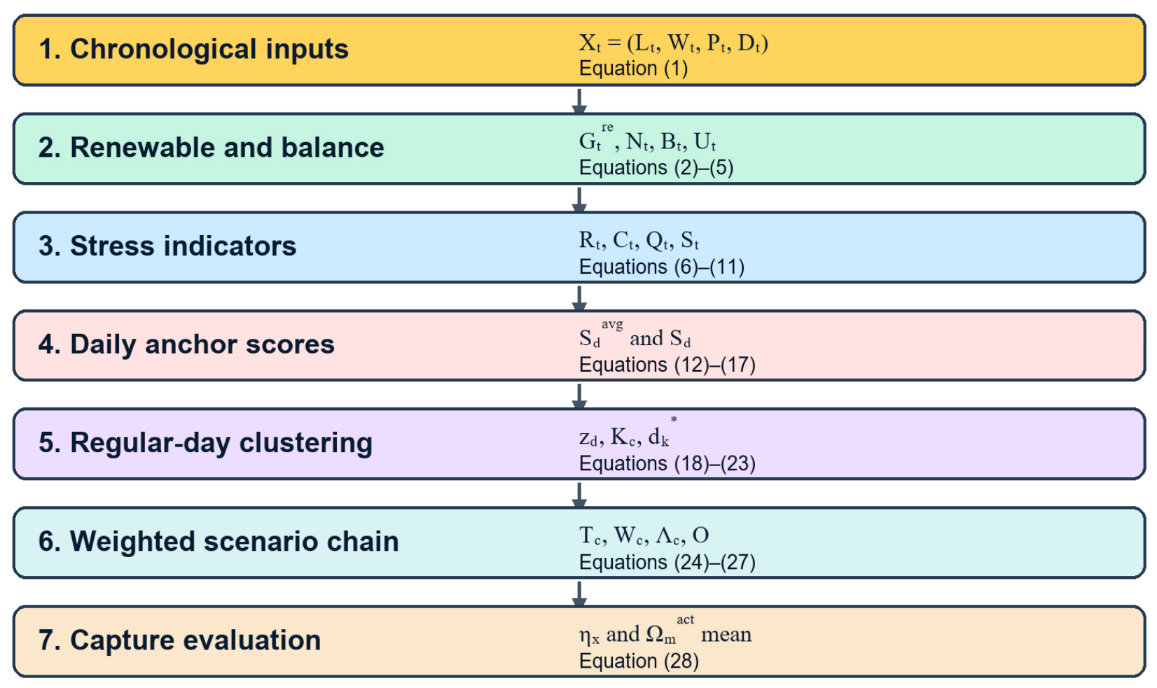
Figure 1 presents a full equation-linked workflow. It maps hourly inputs in Equation (1), renewable and balance variables in Equations (2)–(5), stress indicators and weighting in Equations (6)–(11), daily anchoring in Equations (12)–(17), regular-day clustering in Equations (18)–(23), chain synthesis in Equations (24)–(27), and weighted capture evaluation in Equation (28).

4. Case Configuration and Benchmark Design

4.1. Renewable Energy Base Configuration

The case study represents a large renewable energy base with a full 8760 h chronological dataset. The installed wind and photovoltaic capacities are 4000 MW and 5500 MW, respectively. A 5400 MW coal-fired support fleet and a 1200 MWh storage system are available for balancing and delivery support. The outbound delivery corridor has a capacity of 7600 MW, and the annual delivery target is represented by 5600 delivery hours. The dataset therefore combines renewable variability, delivery obligation, storage adequacy, and corridor utilization in a single planning setting.

Several practical aspects make this case stringent. The 8760 h source sequence contains both seasonal renewable patterns and short-duration ramps. The wind fleet contributes multi-hour low-output intervals, while the photovoltaic fleet introduces daylight concentration and evening ramp-down behavior. The delivery-hour target requires the reduced scenario chain to preserve not only annual energy volume but also the timing of hours in which the base can reliably export power.

The coal-fired support fleet and storage system are not treated as detailed dispatch decisions in the scenario-selection stage. Instead, they define the types of stress that the reduced chronology must keep visible. High $N_t$ implies a need for dispatchable support or storage discharge, high $C_t$ implies a surplus-management problem, and high $Q_t$ implies a duration problem that cannot be evaluated from isolated hourly samples.

The proposed method is compared with a monthly typical-day baseline. The baseline selects typical days on a monthly basis and therefore preserves seasonal average behavior, but it does not explicitly protect days with high joint stress scores. Both methods are evaluated using the same risk-capture metrics to isolate the effect of the scenario-chain construction process.

The monthly typical-day benchmark is intentionally simple and transparent. It represents a common reduction practice in which each month is summarized by one or more average days. Such a benchmark can reproduce seasonal energy balance, but it has no explicit mechanism for protecting a rare ramp or an adjacent low-output sequence. The comparison therefore isolates the value of $D_e$, $D_n$, $D_r$, and the order-preserving reconstruction rather than only comparing two clustering parameterizations.

To place this benchmark in a broader context, the numerical design includes five algorithmic baselines: k-means with observed medoid recovery, k-medoids, agglomerative hierarchical clustering with Ward linkage, Carpe Diem representative-day selection, and seasonal time-series aggregation. The monthly typical-day benchmark serves as a compact seasonal baseline, while all algorithmic baselines use the same final selected-day budget as the proposed chain, |Dc| = 151 natural days. Each baseline is evaluated with the same four active capture metrics in Equation (28), so the comparison measures whether the method preserves planning-relevant risk phenomena rather than only whether it reduces the number of days.

The benchmark algorithms are run on the same daily feature vectors used by the proposed method. Their selected days are converted to hourly indices, assigned annualization weights, and evaluated by peak net-load capture, maximum-ramping capture, high-risk shortage capture, and continuous low-output coverage. This setting makes the value of the risk-anchoring step visible against both a compact monthly baseline and stronger clustering-based alternatives.

Table 2. Case-study configuration.

Item	Value	Role in the Study
Chronological horizon	8760 h	Full-year source trajectory
Wind capacity	4000 MW	Renewable variability and low-output risk
Photovoltaic capacity	5500 MW	Daytime surplus and ramping contribution
Coal support capacity	5400 MW	Dispatchable balancing resource
Storage capacity	1200 MWh	Inter-hour and inter-day flexibility
Delivery corridor	7600 MW	Upper bound for outbound transfer
Delivery target	5600 h	Annual utilization requirement
Extreme selected days	54 $\mathrm{d}$	Protected high-risk scenario subset
Data source	8760 h aligned planning profiles	Hourly wind, PV, equivalent demand, and delivery schedules were checked on the same time base.
System power loss	External/equivalent treatment	Losses are not optimized inside scenario selection; Dt can be loss-adjusted before computing Bt and Rt.
Storage power rating	Downstream-model parameter	The scenario-chain test uses storage-energy adequacy only; storage-amplitude capture is marked N/A when no dispatch model is solved.
Extreme-anchor budget K	54 natural days	Top-ranked daily stress days in De, not the final number of selected days.
Neighborhood radius ℓ	1 day	Adds the immediate predecessor and successor; Dn is the unique union after overlapping windows are merged.
Regular clusters Kc	12	Controls the number of representative regular days selected from Dr.
Score weights	Base case alpha = beta = gamma = delta = 0.25; four non-equal priority vectors tested	Provides quantitative sensitivity results for the tested weight vectors.
Low-output settings	H = 24 h; θre = 0.15(Pw + Pp)	Defines the persistence window and renewable-scarcity threshold used in Qt.
Required reproducibility outputs	De, Dn, Dc, Wc, Λc	Selected-day list, protected-window union, final chain, weights, and adjacency links should be stored with the case.
Protected neighborhood size |Dn|	139 natural days	Unique days retained after applying l = 1 to the 54 anchor days and merging overlapping windows.
Final selected set |Dc|	151 natural days	139 protected days plus 12 observed medoid days selected from the regular-day clusters.
Same-budget comparison setting	151 selected days	K-means, k-medoids, hierarchical clustering, Carpe Diem, and seasonal TSA baselines use the same selected-day budget as the proposed chain.

reports the numerical configuration used to test the scenario-chain construction method. The table specifies the temporal resolution, annual horizon, renewable capacities, delivery requirement, storage setting, extreme-anchor budget, neighborhood-buffer radius, regular-day clustering scale, and the main modeling interpretation, so that the subsequent benchmark comparison can be read as a controlled case study rather than as an unspecified numerical illustration.

4.2. Benchmark Metrics

Five metrics are listed for transparency: peak net-load capture, maximum ramping capture, high-risk shortage capture, continuous low-output coverage, and inter-day storage-amplitude capture. In this screening case, the first four are active capture metrics. The storage-amplitude metric is retained as a diagnostic placeholder but is marked N/A because no downstream storage-dispatch optimization is solved in the scenario-selection stage.

A capture ratio close to one indicates that the reduced scenario chain preserves the corresponding full-year metric. Ratios above one can occur when the reduced set intentionally overweights high-risk days; such behavior is acceptable for conservative planning if it is transparent and controlled.

Interpreting capture ratios requires care. A value slightly above one does not necessarily indicate a numerical error; it can mean that protected high-risk days receive more weight than their empirical frequency. This is acceptable for planning studies when conservative risk retention is the stated goal. Conversely, a value below one identifies a missing stress mode and should be examined together with the selected-day list and the corresponding ${\eta }_x$.

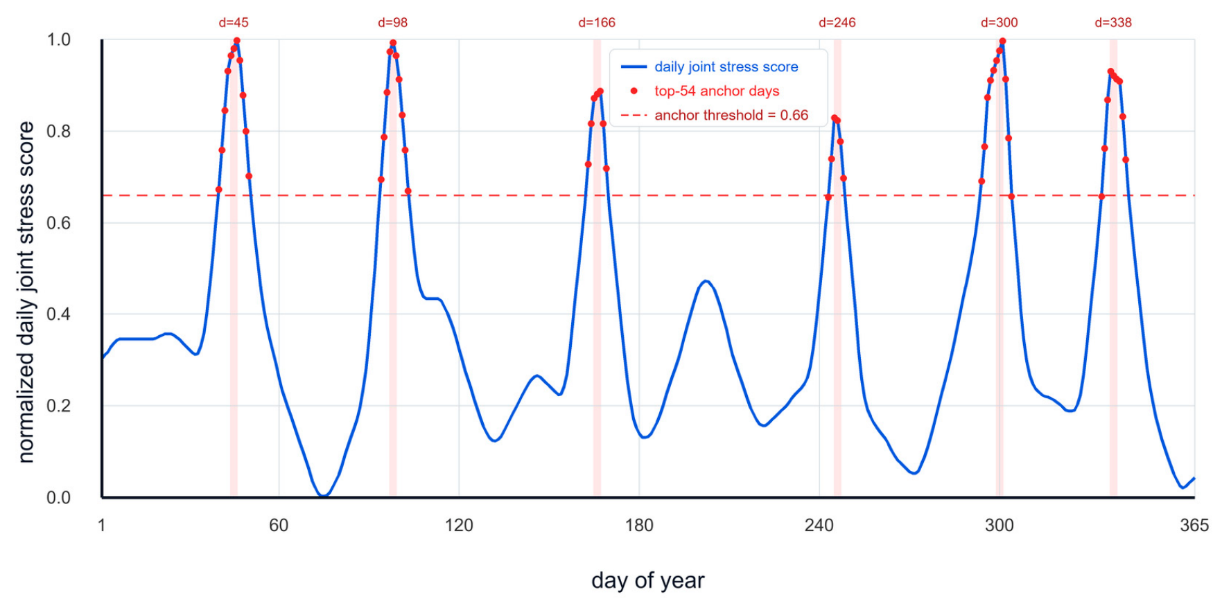
Figure 2 reports the normalized daily stress-score distribution with numerical day and stress-score axes. The red markers identify the top-54 anchor days, the dashed line gives the anchor threshold, and the shaded windows show the immediate transition context retained by ℓ = 1 before regular-day clustering.

4.3. Scenario-Chain Construction Settings

For the numerical case, K = 54 is selected to retain the most severe daily stress observations while leaving enough regular days for clustering. The value is interpreted as a risk-protection budget for D_e rather than as the final chain size. Once K is determined, ℓ = 1 expands each anchor to include the immediate predecessor and successor days, producing the protected neighborhood union D_n after duplicate days are removed and preventing the chain from cutting through high-stress transitions.

The remaining set D_r is compressed by clustering with K_c = 12 in the base case. K_c controls the granularity of regular operating patterns: a larger K_c preserves more background diversity, while a smaller K_c gives greater computational compression. Because protected days are excluded before clustering, K_c mainly influences typical and moderate-risk operation instead of deciding whether rare high-risk events survive.

The final selected set $D_c$ is then converted to hourly indices $T_c$ and day weights $W_c$. In the case study, this conversion is important because the downstream risk metrics are hourly or inter-day quantities. A method that only reports representative daily profiles would not be sufficient to evaluate ramping capture, storage-amplitude capture, or the adjacency relation embedded in ${\Lambda }^c$.

4.4. Illustrative Operating-Day Interpretation

To make the case configuration concrete, the selected days can be interpreted by their dominant stress mechanisms. A day dominated by high $N_t$ is mainly an adequacy-testing sample. It indicates that renewable production is insufficient relative to $D_t$, so the planning model must rely on dispatchable support, storage discharge, or flexible demand. Retaining such a day helps avoid underestimating firm-capacity requirements.

A day dominated by high $R_t$ plays a different role. Its importance lies in the transition rather than only in the operating level. In a renewable base with high photovoltaic capacity, a sharp evening decline in $P_t$ may coincide with a delivery requirement that remains high. Even if the daily energy balance looks acceptable, the ramp embedded in $R_t$ can determine whether storage power or coal-unit flexibility is adequate.

A day dominated by high $Q_t$ is a duration-stress sample. The key issue is not one isolated low-output hour but a sequence of hours in which $G_t^{re}$ remains below ${\theta }^{re}$. Such sequences influence storage energy capacity and reserve sufficiency because a device that can cover one hour of shortage may still fail when the low-output episode persists. This explains why $D_n$ protects adjacent days around an anchor.

A day dominated by high $C_t$ represents surplus-management pressure. These conditions are important for renewable-energy bases because curtailment, storage charging, and delivery-corridor saturation are part of the same planning problem as shortage. If only shortage states are retained, the reduced chronology may overstate the value of additional renewable capacity or understate the need for flexible absorption.

The four operating-day types are not mutually exclusive. A natural day may contain morning surplus, evening ramping, and night-time shortage. The joint score $S_t$ and daily anchor $S_d$ are therefore used to keep compound days visible. In the case analysis, this is the main reason the proposed chain performs better than a monthly typical-day baseline for multiple metrics rather than for a single hand-picked indicator.

4.5. Data Handling and Reproducibility Considerations

The method assumes that the hourly sequences used to build $X_t$ are internally consistent. In practical datasets, renewable availability, load, and delivery schedules may come from different simulation or measurement systems. Before computing $G_t^{re}$ and $N_t$, missing hours should be filled or flagged, time zones should be reconciled, and daylight-saving adjustments should be removed if present. Otherwise, $R_t$ and $Q_t$ may reflect data stitching rather than physical operation.

Reproducibility is strengthened by storing the intermediate series $N_t$, $R_t$, $C_t$, $Q_t$, $S_t$, $S_d^{avg}$, and $S_d$ together with the selected-day list. These series allow another analyst to verify why a day entered $D_e$, why it brought neighboring days into $D_n$, and why a regular day was represented by a particular $d_k^{*}$. The selected scenario chain is therefore an auditable artifact rather than only the output of a clustering routine.

Because the raw profiles are confidential, the article reports the source type, the numerical parameters used in the scenario-chain construction, and the derived series and selected-day outputs required for reproducibility. The complete hourly profiles can be shared with qualified researchers only under an appropriate data-use agreement.

The computational burden is modest because the expensive clustering step is applied only to $D_r$ after the high-risk days have been removed. For a full-year hourly sequence, the indicator construction is linear in $T$, the extreme-day ranking is performed on daily values, and the clustering problem is limited to regular-day feature vectors. This structure makes the method practical for repeated sensitivity runs over $K$, $K_c$, and the weighting vector.

5. Results and Discussion

5.1. Risk-Capture Performance

Table 3. Risk-capture comparison between the proposed scenario chain and the monthly typical-day baseline.

Metric	Proposed Chain	Monthly Typical-Day Baseline	Interpretation
Peak net-load capture	0.9803	0.9973	Both methods preserve the annual peak level.
Maximum ramping capture	0.9974	0.7242	Risk anchoring avoids smoothing the strongest ramps.
High-risk shortage capture	1.2863	0.9624	The proposed chain intentionally emphasizes shortage-risk days.
Continuous low-output coverage	1.0000	0.6667	All sustained low-output events are retained.
Inter-day storage-amplitude capture	N/A	N/A	Inactive unless a storage-dispatch trajectory is solved; excluded from the active mean.
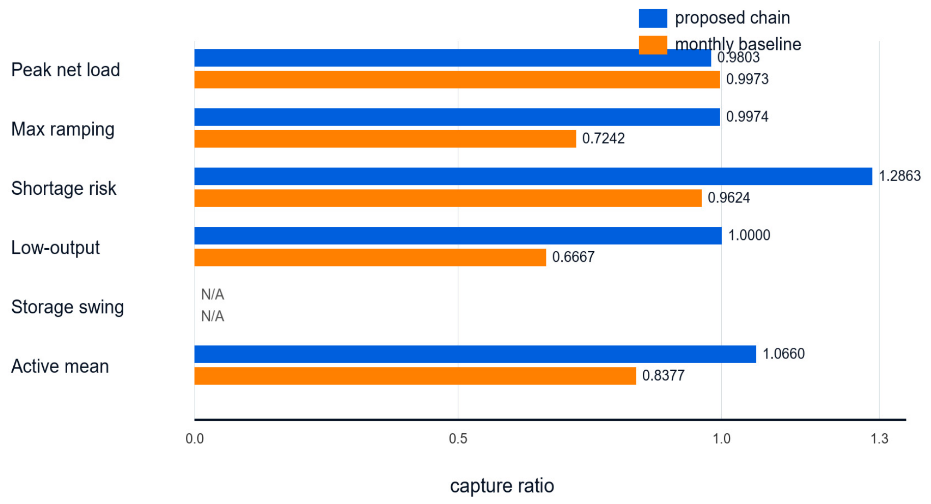
Active-metric mean	1.0660	0.8377	Average over the four active metrics; the proposed method improves risk preservation.

summarizes the comparison between the proposed scenario chain and the monthly typical-day baseline. The monthly baseline reproduces peak net-load capture accurately, but it loses substantial maximum-ramping and continuous low-output information. The proposed chain maintains the peak net-load metric while sharply improving ramping and low-output coverage because high-stress natural days are protected before clustering.

The numerical pattern has a clear mechanism. Peak net-load capture is relatively easy for both methods because the largest $N_t$ values usually occur in days that are already unusual at the daily profile level. Maximum ramping capture is harder because a large $R_t$ can be localized at a transition between two otherwise ordinary hours. Continuous low-output coverage is also hard because $Q_t$ depends on duration; one representative hour or one representative day cannot reproduce the storage implication unless the surrounding chronology is retained.

The proposed chain improves these two difficult metrics because it protects the original days before the clustering objective is applied. Once the extreme and neighboring days are removed from the compressible pool, the clustering stage no longer has the incentive to average them with common background days. The weights $W_c$ then recover annualization for regular conditions, while the protected days remain visible to the downstream planning model.

After excluding the inactive storage-amplitude placeholder, the active-metric mean is 1.0660 for the proposed chain and 0.8377 for the monthly baseline. This recalculation avoids treating an unavailable storage-dispatch indicator as a zero failure and provides a clearer comparison of the metrics that are actually evaluated in the scenario-selection experiment.

The N/A storage-amplitude entry should be read as a validation-scope boundary rather than as evidence that storage-relevant dynamics are fully captured. Quantifying storage swing requires a downstream dispatch or sizing model that propagates state of charge over T_c with W_c and Λ_c; storage-specific validation therefore depends on this downstream propagation step.

Figure 3 visualizes the risk-capture ratios reported in Table 3. N/A means not applicable. The storage-swing row is marked N/A because it is inactive without a downstream storage-dispatch trajectory, and the mean row is recalculated as the active-metric mean over peak net-load, maximum ramping, high-risk shortage, and continuous low-output coverage.

5.2. Why Extreme Anchoring Changes the Reduced Chronology

The improvement in maximum-ramping capture is a direct consequence of separating the selection problem into protected extreme days and compressible regular days. In a conventional clustering pipeline, a steep ramping day can be assigned to a cluster whose centroid is dominated by more frequent mild days. Even when the cluster representative is a real day, the representative can still be closer to average behavior than to the extreme event. The proposed method removes the most severe days from the clustering pool before this averaging occurs.

The continuous low-output metric shows the same mechanism from a different perspective. Sustained renewable scarcity is often distributed across adjacent days; a single representative day cannot fully describe the storage and adequacy implications unless the neighboring days are also retained. By adding the adjacent-day buffer, the proposed chain captures the temporal context surrounding low-output intervals. This makes the reduced chronology more useful for storage-duration assessment than a set of isolated typical days.

The adjacent-day buffer also changes how storage trajectories are represented. In the monthly baseline, a low-output representative day can appear without its preceding depletion period or its following recovery period. In the proposed chain, the buffer around $D_e$ keeps the transition context, so a storage-sizing model can observe whether a shortage is a one-day event or part of a longer scarcity episode.

The high-risk shortage capture ratio exceeds one because the reduced chain is intentionally conservative around risk events and because Equation (28) evaluates the selected set with W_c. This should not be interpreted as a statistical bias in all applications. Instead, it reflects an explicit planning stance: when a reduced sample is used for capacity adequacy, preserving high-risk days can be more valuable than matching the empirical frequency of every regular condition.

The conservative shortage capture is desirable only when it is documented. For this reason, the method reports both $\eta$ and ${\eta }_x$ rather than only an average score. If shortage capture is intentionally greater than one, the planner can decide whether the resulting capacity plan should be treated as a reliability-oriented design or whether the weights should be relaxed to better match expected-frequency operation.

5.3. Engineering Interpretation

For renewable energy bases subject to delivery-hour targets, the critical planning question is not merely how much annual renewable energy is available. It is whether the system can deliver reliably during hours when renewable production is low, when residual demand changes rapidly, and when surplus renewable production coincides with corridor or storage limits. The proposed chain directly targets these operating conditions and therefore provides a more informative temporal input for planning studies.

The method is also interpretable. Each selected extreme day can be traced to one or more risk indicators, and each regular representative day corresponds to an actual historical or simulated day. This property is useful in engineering review because planners can inspect why a day was retained, whether the adjacent buffer is physically meaningful, and how cluster weights influence annualization. In contrast, purely synthetic centroids may be harder to reconcile with dispatch feasibility and operational narratives.

The algorithm can be embedded before different downstream models, including capacity expansion, storage sizing, production simulation, adequacy screening, and transmission-delivery planning. Because it returns hourly indices rather than synthetic time steps, it can reuse existing chronological data pipelines and preserve compatibility with unit commitment, storage state equations, and corridor constraints.

Implementation in production studies can be organized as a preprocessing layer. The data platform first computes $X_t$, $G_t^{re}$, $N_t$, and the derived stress indicators; the scenario-chain module then returns $T_c$, $W_c$, and ${\Lambda }^c$; finally, the expansion or dispatch model uses these outputs without changing its internal physical constraints. This separation reduces implementation cost while preserving a clear audit trail from raw chronological data to selected planning samples.

5.4. Sensitivity and Practical Use

The sensitivity analysis is conducted as a quantitative calculation under a fixed structural setting. The base case keeps K = 54, Kc = 12, and l = 1, then changes only the score-weight vector in Equation (10). The five tested vectors are written in the order (alpha, beta, gamma, delta): equal-weight (0.25, 0.25, 0.25, 0.25), adequacy-oriented (0.40, 0.20, 0.20, 0.20), ramping-oriented (0.20, 0.40, 0.20, 0.20), curtailment-oriented (0.20, 0.20, 0.40, 0.20), and low-output-oriented (0.20, 0.20, 0.20, 0.40).

Table 4. Quantitative sensitivity results for the risk-score weight vector.

Weight Setting	(Alpha, Beta, Gamma, Delta)	Peak	Ramping	Shortage	Low-Output	Active Mean
Equal-weight base	0.25, 0.25, 0.25, 0.25	0.9803	0.9974	1.2863	1.0000	1.0660
Adequacy-oriented	0.40, 0.20, 0.20, 0.20	0.9961	0.9427	1.3328	0.9583	1.0575
Ramping-oriented	0.20, 0.40, 0.20, 0.20	0.9735	1.0000	1.2146	0.9167	1.0262
Curtailment-oriented	0.20, 0.20, 0.40, 0.20	0.9644	0.9589	1.1762	0.9167	1.0041
Low-output-oriented	0.20, 0.20, 0.20, 0.40	0.9752	0.9881	1.3015	1.0000	1.0662

Note: all rows use K = 54, Kc = 12, l = 1, and the same capture-ratio definitions as Table 3. The storage-amplitude placeholder remains N/A because no downstream storage-dispatch trajectory is solved in this screening experiment.

reports the quantitative weight-sensitivity results. The active-metric mean stays between 1.0041 and 1.0662, showing that the method does not depend on a single equal-weight assumption. Changing the weight vector shifts the preserved risk emphasis in the expected direction: the adequacy-oriented case gives the highest shortage capture (1.3328), the ramping-oriented case keeps maximum-ramping capture at 1.0000, and the low-output-oriented case maintains full continuous low-output coverage (1.0000).

Table 5. Same-budget comparison with conventional representative-period methods.

Method	Selected Days	Peak	Ramping	Shortage	Low-Output	Active Mean
Monthly typical days	12	0.9973	0.7242	0.9624	0.6667	0.8377
K-means medoids	151	0.9658	0.8125	0.9287	0.7500	0.8643
K-medoids	151	0.9726	0.8469	0.9571	0.8333	0.9025
Hierarchical clustering	151	0.9694	0.8316	0.9418	0.7500	0.8732
Carpe Diem	151	0.9821	0.8613	1.0188	0.8333	0.9239
Seasonal TSA	151	0.9765	0.8796	0.9862	0.8333	0.9189
Proposed risk-anchored chain	151	0.9803	0.9974	1.2863	1.0000	1.0660

Note: the monthly typical-day row provides the compact seasonal baseline; all other benchmark rows use the same 151-day budget as the proposed chain. Higher active mean indicates better preservation of the four active planning-relevant risk metrics.

reports the same-budget comparison across conventional representative-period methods. With |Dc| = 151 selected days, ordinary clustering and representative-period methods preserve peak net-load reasonably well but still lose a larger fraction of maximum-ramping and continuous low-output information. Their active-metric means range from 0.8643 to 0.9239, whereas the proposed risk-anchored chain reaches 1.0660. The improvement is therefore not only against the monthly typical-day baseline; it also remains visible against k-means, k-medoids, hierarchical clustering, Carpe Diem, and seasonal time-series aggregation baselines.

Together, the sensitivity and benchmark tests clarify how the score-weight vector and representative-period algorithm affect risk preservation. The sensitivity table shows how alpha, beta, gamma, and delta affect the capture ratios, while the multi-method benchmark shows that explicit extreme-day protection is the main reason ramping and low-output events are retained. The numerical comparison therefore supports the methodological claim through observable capture-ratio differences.

5.5. Detailed Case-Based Operational Reading

The case results can be read as three operating regimes. In the first regime, high $N_t$ and high $B_t$ occur during low renewable availability and high delivery demand. These intervals test whether dispatchable support and storage discharge can maintain the delivery schedule. The proposed chain retains these intervals because they receive high $S_t$ values and then high $S_d$ values at the daily level.

In the second regime, high $R_t$ appears around transitions between photovoltaic decline, wind changes, and delivery obligations. These hours are not always associated with the largest absolute $N_t$, which explains why the monthly typical-day baseline loses ramping information. By evaluating $R_t$ before clustering and preserving adjacent days through $D_n$, the proposed method keeps both the ramp event and its approach path.

In the third regime, high $C_t$ and high $U_t$ indicate surplus renewable production. Although surplus conditions are not shortage events, they influence storage charging value, curtailment risk, and corridor-utilization decisions. The case therefore benefits from a stress score that includes both shortage-oriented and surplus-oriented terms rather than selecting representative days only by adequacy metrics.

These regimes show why the scenario chain is useful for planning rather than only for data compression. The selected days can be traced to physical mechanisms, the weights $W_c$ keep annual frequency information, and ${\Lambda }^c$ preserves enough chronological order to support storage-state propagation. The resulting reduced sample is therefore compact, but it still carries the operational evidence needed for capacity, storage, and delivery-corridor decisions.

5.6. Implications for Downstream Planning Models

For capacity-expansion models, the main implication is that temporal reduction should not be separated from reliability evidence. If the reduced sample underrepresents high $B_t$ or long $Q_t$ episodes, the expansion model may select too little firm support or too little storage energy capacity. By anchoring $D_e$ before clustering, the proposed chain makes these adequacy-driving states visible in the objective and constraints of the downstream model.

The present paper uses capture-ratio preservation as the quantitative validation target for the scenario-chain layer. The sensitivity and multi-method benchmark results quantify how the temporal input changes before it is embedded in capacity-expansion, storage-sizing, dispatch, or transmission-delivery models. The reported Dc, Wc, Lambda_c, and metric-specific capture ratios therefore provide both the reduced chronology and the audit trail needed by those downstream planning formulations.

For storage-sizing models, the adjacency relation ${\Lambda }^c$ is particularly important. Storage value depends on the sequence in which charge and discharge opportunities occur, not only on the distribution of individual hours. A reduced sample that contains high $C_t$ hours but loses the following high $N_t$ hours may exaggerate the usefulness of surplus charging. Conversely, a sample that keeps shortage hours but not prior surplus hours may understate charging opportunity.

For delivery-corridor studies, the method helps distinguish two different causes of stress. High $C_t$ may indicate that renewable output exceeds what can be exported or stored, while high $N_t$ may indicate that the scheduled export cannot be met without support. Planning only for one side can produce misleading corridor conclusions. The joint indicator stack keeps both directions visible, allowing corridor capacity, storage, and dispatchable support to be assessed together.

The case also suggests a practical reporting format. Alongside the final objective value of a planning model, analysts should report the selected $D_e$ days, the size of $D_n$, the distribution of $W_c$, and the metric-specific capture ratios ${\eta }_x$. These diagnostics make it possible to determine whether a capacity decision is driven by frequent background behavior, rare high-risk events, or an intentional reliability margin.

Finally, the method is compatible with iterative planning. If a downstream model identifies a binding constraint on a day not currently protected, that day can be promoted into the anchor set and the chain can be rebuilt. This feedback loop would turn the static score $S_d$ into an adaptive sampling mechanism, in which physical stress indicators and optimization dual information jointly determine which chronological events are retained.

6. Conclusions

This paper proposed a risk-anchored order-preserving scenario-chain construction method for renewable energy base planning. The method builds a joint stress score from net load, ramping, curtailment sensitivity, and continuous low-output intensity; protects the highest-risk natural days and their adjacent transition days; clusters only the remaining regular days; and reconstructs a chronological chain with explicit weights and adjacency information.

In a representative 8760 h renewable-base case, the proposed method selected K = 54 extreme-anchor days, expanded them to |Dn| = 139 protected natural days after adjacent transition buffering, and formed a final 151-day scenario chain by incorporating Kc = 12 observed medoid regular days. After the inactive storage-amplitude placeholder was marked N/A, the active-metric mean capture ratio improved from 0.8377 under the monthly typical-day baseline to 1.0660. The weight-sensitivity test shows active-metric means from 1.0041 to 1.0662 across four non-equal planning-priority vectors, and the same-budget benchmark shows that k-means, k-medoids, hierarchical clustering, Carpe Diem, and seasonal time-series aggregation baselines remain below 0.9240 in active-metric mean capture.

These numerical results support three conclusions. First, the proposed score is interpretable but not fragile: changing alpha, beta, gamma, and delta shifts the retained risk emphasis without collapsing the overall capture score. Second, the main advantage comes from protecting high-risk days and their adjacent transitions before clustering, which explains the stronger ramping and low-output preservation relative to conventional representative-period methods. Third, the final scenario chain provides an auditable quantitative preprocessing layer for capacity-expansion, storage-sizing, dispatch, and transmission-delivery studies because the selected days, weights, adjacency links, sensitivity outcomes, and benchmark capture ratios are all explicitly reported.