Article

Mitigating Systemic Risks in the Energy Transition: A Comparative Study of Weather and Solar Irradiance Forecast Providers Based on Real-World Performance

by
Giovanni Spinelli
1,
Gabriele Piantadosi
2,
Sofia Dutto
3,*,
Saverio De Vito
2 and
Girolamo Di Francia
2,*
1
ENEA Casaccia Research Centre, Energy Technologies and Renewable Sources Department (TERIN), 00123 Rome, Italy
2
ENEA Portici Research Centre, Energy Technologies and Renewable Sources Department (TERIN), 80055 Portici, Italy
3
Department of Electrical Engineering and Information Technology (DIETI), University of Naples Federico II, 80125 Naples, Italy
*
Authors to whom correspondence should be addressed.
Energies 2026, 19(14), 3361; https://doi.org/10.3390/en19143361
Submission received: 21 June 2026 / Revised: 10 July 2026 / Accepted: 13 July 2026 / Published: 16 July 2026

Abstract

The transition towards decarbonised energy systems, often characterised by high photovoltaic penetration, imposes crucial challenges for operational security, flexibility and grid resilience. In this landscape, meteorological-data reliability has emerged as a strategic pillar to mitigate systemic risks arising from forecasting uncertainty, including grid imbalances, electricity-market volatility, and structural asset safety during extreme weather. This study provides a comparative analysis of four forecasting providers, evaluating their accuracy across atmospheric and solar irradiance parameters through heterogeneous datasets spanning diverse climatic zones and seasons. The analysis is performed by employing a dual-source validation framework that benchmarks every forecast against independent, real-world references rather than the providers’ own model-derived observations: first, the atmospheric variables are compared with real surface-station measurements; second, plane-of-array irradiance is benchmarked directly against on-site sensors at operational photovoltaic plants. This dual-source approach isolates systematic model biases relative to real-world environmental conditions, yielding a provider-independent estimate of accuracy against the true atmospheric and irradiance state. This work therefore proposes not merely a comparative analysis but a validation methodology that addresses a specific limitation of existing forecast-comparison approaches, offering actionable insights to minimise financial and operational risks while fostering a secure, resilient, and sustainable energy infrastructure.

1. Introduction

For over a century, the global energy model has been based on, and continues to rely heavily on, fossil fuels such as coal, oil, and natural gas. However, it is clear that this paradigm has become unsustainable in several respects, starting with the pressing climate crisis. The rise in global temperatures is caused mainly by the increase in atmospheric CO2 concentrations as a result of human activities, including fossil fuel combustion and deforestation [1]. This environmental emergency is accompanied by systemic geopolitical issues, as the concentration of reserves in specific areas (such as gas in Russia or oil in the Middle East and Venezuela) transforms energy into a tool for blackmail, sanctions, and conflicts [2,3,4] with the additional effects on price volatility in global markets [5], including for food commodities, as exemplified by the severe impact of the Russia-Ukraine conflict on global food security [6]. Last but not least is the impact on public health and safety, as air pollution from energy production and transportation remains one of the main causes of respiratory diseases [7] globally, while high atmospheric energy events are frequently hitting vulnerable territories and communities.
For all these reasons, a transition to clean energy now appears essential, with photovoltaics playing a leading role as a fundamental pillar of change. However, its large-scale deployment still faces critical challenges related to resource management. Energy production is governed by variables acting on different levels: the availability of the primary resource and operational efficiency. This is particularly evident for variable renewable energy (VRE) sources, including photovoltaic (PV) and wind energy. While theoretical production depends directly on irradiation, and is therefore closely linked to the alternation of day and night and to cloud cover, the real PV output also responds to environmental drivers, temperature and humidity in particular, which cause fluctuations in power output even under identical irradiation. It is therefore essential to analyse these dynamics separately for accurate modelling.

1.1. Sources of Uncertainty in Renewable Integration and the Role of Forecasting

Feeding renewable generation into a modern power system raises well-known difficulties tied to forecasting uncertainty, a theme addressed systematically by Borggrefe and Neuhoff (2011) [8] in their study on the design of balancing and intraday markets for wind integration. The authors identify three principal sources of forecasting error, which together determine the overall demand for balancing power in an electricity system: demand uncertainty, uncertainty of the (wind) generation, and the sudden failure of production plants. Although the explicit reference is to wind energy, it is worth stressing from the outset that the “wind source” can here be regarded as a proxy for any weather-dependent energy source: the treatment therefore extends to the entire spectrum of non-dispatchable renewables, and in particular, to photovoltaics, whose producibility is strictly tied to solar irradiance and cloud cover.

1.1.1. Demand Uncertainty

A first source of uncertainty is associated with demand, that is, load volatility: even without renewable generation, consumption depends on weather conditions, consumer habits, economic activity and hard-to-anticipate exceptional events. This is probably the hardest source to control, constituting the system’s “baseline” uncertainty on which renewable-driven variability is superimposed. Demand Response techniques extended to individual consumers offer a promising short-to-medium-term mitigation: Chatuanramtharnghaka et al. (2024) [9] show how demand-side flexibility dampens load volatility and stabilises the grid, while a PRISMA-2020 review of Demand Response forecasting [10] highlights probabilistic consumer-behaviour modelling as the key to reducing residual load uncertainty.

1.1.2. Failure of Production Plants

A second source is the failure of production plants, the sudden unavailability of generating units. Unlike demand uncertainty, this component is markedly asymmetric: failures almost always cause a supply deficit, requiring adequate positive reserves for rare but severe events. Progress here comes mainly from anomaly detection for predictive maintenance: the comprehensive review by Apata et al. (2026) [11] documents the maturity of unsupervised methods (in particular, autoencoders and principal component analysis) for anomaly detection under label-scarce conditions, tools that help anticipate failures and compress this deficit tail.

1.1.3. Uncertainty of Weather-Dependent Generation

The last source, central to the present treatment, is the uncertainty of (wind) generation, here taken as the paradigm of any weather-dependent source. The power produced by a wind farm depends non-linearly on wind speed, an intrinsically stochastic quantity that is difficult to predict accurately over extended horizons. Analogously, in the PV case, production is governed by irradiance, subject to fluctuations caused by the transit of clouds, by seasonality and by atmospheric phenomena. Here too the error distribution is essentially symmetric, with the possibility of both under-production and over-production relative to expectations. It is precisely this component that makes renewable integration particularly onerous for the grid operator, since its impacts potentially grow with the penetration of non-dispatchable sources in the energy mix. The symmetric nature of wind and PV uncertainty implies the need for balancing reserves in both directions, positive and negative. For this element, as discussed below, strong improvements are required in the optimal use of satellite data and in the treatment of data obtainable from the various providers. In this respect, the review by Jiao and Xiao (2025) [12] on data-driven approaches for time-series solar irradiance forecasting shows how convolutional networks, combined with satellite imagery, allow the spatial features of cloud formations to be extracted, appreciably improving very-short-term forecasts, while hybrid models integrating satellite imagery, numerical weather prediction (NWP) and ground measurements achieve today the highest accuracy.

1.1.4. Synthesis and Perspective

The superposition of these three distributions determines the overall balancing-power demand of the system. Borggrefe and Neuhoff [8] show how, once an acceptable deficit level is fixed (e.g., 0.1%), it is possible to size the required positive and negative reserve capacities, distinguishing between expected positive and negative balancing power and the reserve capacity at the tails of the distribution. This probabilistic framing is consistent with the most recent literature on renewable forecasting: Antonanzas et al. (2016) [13], in their broad review of solar-power forecasting methods, show how a reduction in the forecast error translates directly into lower balancing costs and greater system reliability. Likewise, Wang et al. (2019) [14] emphasise how modern deep-learning techniques allow the uncertainty associated with PV and wind generation to be progressively compressed, attenuating the amplitude of the error distributions described by Borggrefe and Neuhoff and consequently reducing the reserve requirement. In this perspective, the improvement of forecasting accuracy represents the most effective lever to make the massive integration of renewable sources economically and technically sustainable.

1.2. Reliable Weather Providers as a Strategic Requirement

The need for reliable weather providers, both in the short and long term, is therefore crucial for a number of operational and strategic reasons. Accurate data is essential to keep the grid stable by holding supply and demand continuously in balance, while data-stream integrity remains a security priority: anomaly detection techniques are essential to identify corrupted or malicious measurements in energy microgrids [15]. The EU electricity market operates across interconnected segments with distinct time horizons. The Day-Ahead Spot market accepts hourly buy/sell bids for the following day, while the Intraday segment manages near-real-time deviations at 15 or 30 min intervals. Precise forecasting enables producers to meet feed-in commitments, avoiding balancing-market penalties [13,16,17] from production deviations. Economically, forecast reliability stabilises markets and reduces financial risks for investments and trading.
Meteorological accuracy is crucial not only for trading but also for the physical safety of the plants: high-quality weather forecasting plays a key role in enhancing system preparedness and boosting the resilience of integrated energy infrastructures during severe weather anomalies, facilitating the optimal deployment of flexible grid resources [18,19]. At the same time, proper planning promotes environmental sustainability by minimising reliance on polluting backup plants when renewable output is predictable. Long-term forward-market planning (monthly to yearly scales) optimises maintenance and lifecycle management, allowing operators to assess global warming impacts on radiation and asset yield [20] and schedule technical interventions during low-efficiency periods. In this dynamic market, precise feed-in planning is mandatory to prevent imbalances and financial losses. Comparing weather providers is therefore a critical operational necessity, as forecast inaccuracies directly cause significant electricity production errors [20,21]. However, existing benchmarking studies typically compare providers against each other or validate forecasts using providers’ own historical products [13,21]. Since these references rely on reanalysis and gap-filling models, they measure internal consistency rather than true atmospheric accuracy and cannot isolate shared error components. The core scientific gap addressed here is the absence of a validation protocol using a reference layer physically independent of all tested providers. To address this complexity, the study employs a dual-source validation framework that independently tests atmospheric parameters and solar irradiance against ground-truth measurements. These two comparisons are independent and run in parallel: the atmospheric forecasts are benchmarked against real surface-station observations distributed across the climatic zones considered, while the irradiance forecasts are compared directly with on-site sensors installed at operational PV plants. This independent structure enables the identification of systematic model biases relative to actual environmental conditions, ensuring a robust assessment of forecast reliability across different climate zones.
Given the direct correlation between PV output, ground solar radiation, and instantaneous meteorological variables (e.g., cloud cover, humidity) [21], accurate weather evaluation is fundamental to energy forecasting quality. This work analyses multiple providers to verify their reliability and forecast generalisability [13,22]. The primary objective is to establish a transparent, reproducible methodology based on openly accessible reference data and fully documented acquisition procedures. By utilising public references and standard provider APIs instead of proprietary intermediates, this approach enables widespread forecast verification for researchers and prosumers alike, strengthening transparency across the energy-data ecosystem.

1.3. A Preliminary Observation: Forecast Error and Grid Imbalance

To ground the preceding considerations in operational evidence, we carried out a preliminary analysis linking the irradiance forecast error to the actual imbalance of the national grid. The analysis combines two independent and entirely real data sources. The first is the on-site, plane-of-array (PoA) irradiance measured by physical sensors installed at a set of spatially distributed, operational Italian PV plants used in this study [21], evaluated against the day-ahead irradiance forecasts of Provider-1 and Provider-3 (the only two services in the sample exposing an irradiance product). The second is the aggregate zonal imbalance published by the Italian transmission system operator (Terna) for the Southern bidding zone. Aggregate zonal-imbalance and settlement data for the Italian bidding zones are published by Terna S.p.A., the national transmission system operator, through its public reporting portal (https://www.terna.it/ accessed on 16 June 2026), the  macro-area in which the instrumented plants are located.
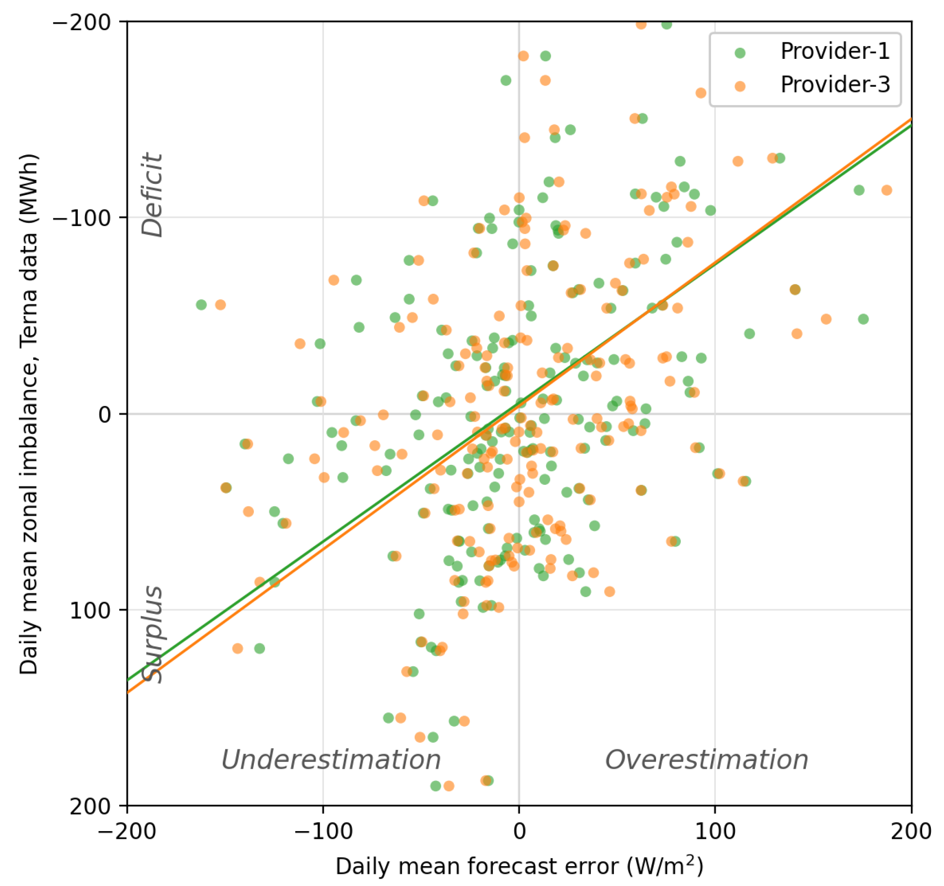
The zonal imbalance is the net deviation, settled by the system operator, between the energy actually injected into and withdrawn from a bidding zone and the corresponding scheduled programme; it therefore aggregates the contributions of all generation technologies and of the load. When the analysis is restricted to daylight hours, as in Figure 1, the weather-dependent variability of this aggregate is dominated by the PV component, whose output is precisely the quantity governed by the irradiance forecast.
A second, and central, observation concerns the origin of the forecast error. Commercial aggregators and “scientific” or institutional providers alike generate atmospheric states by post-processing a small number of global NWP systems, primarily the ECMWF IFS and the NOAA GFS [21]. Global models also underpin the forecasts on which market participants build their day-ahead schedules. As a consequence, a systematic, shared error component that propagates to the grid imbalance is common to the providers and to the operators that set the zonal programme. The empirical pattern shown in Figure 1 is consistent with this interpretation: the two providers, despite being distinct products, yield fitted trend lines that are almost coincident, as the dominant error contribution is shared rather than provider-specific. Moreover, the relationship has a clear and physically sensible direction: a positive mean forecast error, that is an overestimation of irradiance and hence an over-forecast of PV generation, is associated with the zone moving into deficit, whereas an underestimation is associated with a surplus. A linear fit to the points yields slopes of approximately 0.71  MWh of imbalance per W/m2 of daily mean error for Provider-1 and 0.73  MWh per W/m2 for Provider-3; the association is negative in sign, since a positive error maps onto a negative (deficit) signed imbalance, and for readability, the ordinate in Figure 1 is drawn with the deficit pointing upward. The scatter around these fits is nonetheless pronounced, and the coefficient of determination is correspondingly low ( R 2 0.19 for Provider-1 and 0.21 for Provider-3). This is expected and, in itself, informative: the zonal imbalance is the net outcome of many concurrent drivers, physical and natural (forced PV unavailability, the variability of other non-dispatchable renewables such as wind, weather-driven swings in load), technical and grid-related (generator outages, transmission constraints, ramping limits), and economic and regulatory (bidding strategies, cross-zonal exchanges, day-ahead-to-real-time rescheduling, incentive schemes and balancing rules). Figure 1 is therefore not intended to demonstrate a direct, one-to-one relationship between forecast error and imbalance, but to reveal that, beneath this multi-causal variability, a systematic background component linked to the meteorological providers’ forecast error retains a positive and physically coherent association with the zonal imbalance.
This preliminary evidence establishes the gap that the present study sets out to address. The accuracy of the irradiance forecast is not an abstract quality metric: through a shared, systematic error component, it retains a consistent, positive association with the grid imbalance, weak in explained variance but coherent in sign and, once scaled to the energy of an entire bidding zone over many days, non-negligible in the balancing costs and penalties discussed above. Characterising and comparing the providers that feed this chain is therefore a precondition for any strategy aimed at compressing that error and the systemic risk it carries.
Against this background, the contributions of this work are the following. First, we benchmark every forecast, atmospheric and solar alike, against fully independent physical references, surface-station measurements and on-site PoA sensors at operational plants, isolating each model’s true systematic bias. Second, in place of the single aggregate score reported by most studies, we disaggregate performance by season, climate zone, diurnal cycle and forecast horizon across sites spanning all five Köppen–Geiger macro-zones, and we quantify uncertainty with a block bootstrap that separates providers only where their confidence intervals do not overlap; this shows that aggregate metrics can be actively misleading for operational selection, concealing pronounced spatial and seasonal heterogeneity within a single variable. Together, these elements turn a conventional provider comparison into a reusable, statistically grounded assessment protocol for selecting forecast sources under real operating conditions.

2. Weather Data Providers

The rapid technological development and widespread availability of the Internet have made access to meteorological data instantaneous and global, through both free and on-demand services. In this landscape, weather providers act as advanced technological intermediaries, offering digital solutions based on historical, current, and forecast data. Many operators integrate physical-mathematical models with real measurements; a notable example is Open-Meteo, which provides historical series based on reanalysis datasets. These systems combine heterogeneous observations (stations, satellites, radars) to create a consistent atmospheric record [23], using mathematical models for gap-filling in areas lacking physical instrumentation.

Overview of Meteorological Providers

Providers distribute content via web portals, mobile apps, and especially application programming interfaces (APIs), which are essential for automated business integration. This study analyses the reliability and generalizability of leading services, which are not isolated entities but optimise data drawn from the two pillars of global meteorology: the IFS and GFS models.
The IFS (Integrated Forecasting System), developed by ECMWF (European Centre for Medium-Range Weather Forecasts) [21,24], is a coupled Earth-system model whose non-hydrostatic formulation resolves the atmosphere on a vertical, altitude-based coordinate. It delivers hourly updated fields at roughly 14 km resolution. Since 2023 ECMWF has also introduced the experimental machine learning variant AIFS (Artificial Intelligence Forecasting System) [25].
The GFS (Global Forecast System), run by the US NOAA through the National Centers for Environmental Prediction (NCEP) [21], couples atmosphere, ocean, land surface and sea ice components. It forecasts up to sixteen days on a grid of about 28 km, coarsening to roughly 70 km beyond the eight-day horizon.
The modern weather-provider landscape varies significantly in delivery methods, historical-data depth, and local accuracy. While companies like MeteoAM, Tomorrow.io, and Windy focus heavily on web and mobile user interfaces, most operators (including Open-Meteo and Visual Crossing) adopt an API-based approach. To optimise spatial accuracy, Visual Crossing reaches resolutions of 2 km, whereas Open-Meteo uses a proprietary “best match” algorithm to select the morphologically closest grid cell. Providers like Windy and Open-Meteo guarantee total transparency, allowing users to manually select between global and regional models (GFS, ECMWF, ICON). The standard forecast horizon is 14–16 days, but Open-Meteo extends seasonal projections up to three months, offering temporal granularities down to 15 min or even single minutes, shared also by Meteosource and Weather API. Conversely, services like MeteoAM maintain shorter horizons (4–5 days) with lower numerical resolution but rely on proprietary physical measurement networks. Solar irradiance data represents a technical and economic watershed: Visual Crossing and Weather API restrict it to paid endpoints, while Meteoblue and Open-Meteo include it in free tiers, which are universally provided under strict rate limits. Finally, the dual availability of historical observations (provided by OpenWeather, AccuWeather, and WeatherBit) and archived historical forecasts (such as Open-Meteo) is crucial, enabling direct comparison between theoretical forecast accuracy and ground truth. A synoptic overview of the surveyed providers is reported in Table 1.

3. Materials and Methods

3.1. Dataset

Accurate, long-horizon weather forecasts are essential for the energy market. This study compares multiple data providers to assess their reliability across general atmospheric and PV-specific variables. As such, to ensure a heterogeneous evaluation, the services are categorised into four groups based on business model and target audience: Open Source and Research (raw-data transparency and ease of integration), Enterprise Solutions (industrial scalability and infrastructure reliability), Precision Meteorology and Advanced Analysis (high spatial accuracy for localised critical decisions), and Institutional and Public Safety (authoritative, simplified territorial management). One representative was selected per category based on API access, cost, and group representativeness. The four providers are reported anonymously (Provider-1 to Provider-4) for two reasons: several services’ terms of use restrict data redistribution and named benchmarking, and a named ranking from a finite sample (specific sites, a single annual window, particular API configurations) would read as a commercial verdict that is in fact conditional on the evaluation design. Our aim is therefore not a fixed leaderboard but a characterisation of provider archetypes and a transferable evaluation procedure. Each provider is mapped to one of the four categories defined above, with the candidate pool and its delivery characteristics reported in Table 1.
Specifically, Provider-1 represents the open-source sector due to its vast historical archive and strategic high-resolution model blending. Provider-2 represents the industrial tier with an architecture optimised for large-scale business applications. Provider-3 stands for precision meteorology, offering granular microclimate analyses. Finally, Provider-4 embodies the institutional sector, prioritised for its authoritative territorial-safety data and reliable presentation.

3.1.1. Providers’ Weather Data

The core dataset includes forecasts from all four providers (Table 2). The evaluation spans a comprehensive parameter list for Provider-1 and Provider-2: temperature, humidity, pressure, wind speed, and cloud cover (plus precipitation exclusively for Provider-1). Provider-3 and Provider-4 provide more restricted variable subsets: the analysis for Provider-4 covers temperature, humidity, pressure, and wind, while Provider-3 is strictly limited to temperature and wind. The temporal resolution generally ranges from one to three hours, though granularity frequently decreases at extended forecast horizons.
Although Table 2 shows that the four providers differ for forecast horizon, variable category and sampling scheme, every comparison presented in this study is carried out under matched conditions rather than pooling heterogeneous data. All providers and variables are evaluated over the same set of monitoring sites spanning the five Köppen–Geiger macro-zones, so no cross-provider comparison reflects differences in geographic sampling. Within this common set of locations, providers are contrasted only within the same physical variable and for each variable, the forecast-horizon axis is restricted to 120 h. No comparison in this study therefore involves variables, horizons or locations that are not jointly available to the providers concerned. For the conventional atmospheric variables (temperature, wind speed, humidity, sea-level pressure, precipitation and cloud cover) the reference is real surface-station data from the NOAA Integrated Surface Database [26], accessed through the Meteostat service [27] at the station nearest to each site. Across the sites this nearest station lies between 0 and about 31 km away (median close to 12 km, and on-site at five locations), and after cleaning the station series cover at least 94% of the hourly records for every variable. Short gaps of up to three consecutive hours are filled by temporal interpolation, and the residual missing hours are filled from the globally consistent ERA5 reanalysis [23]; this reanalysis-based filling is marginal, affecting below 0.1% of the records at every site except one high-latitude polar station where surface reporting is intermittent. For irradiance, the reference is the on-site sensors at the PV plants.

3.1.2. Providers’ Irradiance Data

In the field of solar radiation, the analysis is limited to two of the four selected providers, as only Provider-1 and Provider-3 integrate radiation forecasts into their services. For the remaining suppliers, these data were excluded as they were only accessible through paid commercial subscriptions, not used at this stage of the study. Of the two, only Provider-1 also provides the corresponding observations, generated through sophisticated physical models and the processing of historical data. The study focuses on three variables fundamental for estimating energy potential: shortwave radiation, the total radiant energy emitted by the Sun; diffuse radiation, the portion reaching the ground after being reflected or deflected by atmospheric particles; and direct normal irradiance (DNI), the solar energy striking a surface kept constantly perpendicular to the incident rays.
These components, integrated together, contribute to determining the Global Horizontal Irradiance (GHI), which expresses the total energy captured by a horizontal surface placed on the ground. The GHI is calculated according to the physical relationship of Equation (1):
GHI = DNI · cos ( θ z ) + DHI
In this formulation [28], GHI represents global horizontal irradiance, θ z the solar zenith angle (the angular deviation between the position of the Sun and the vertical of the location), and DHI the diffuse horizontal irradiance. This approach allows the radiation balance at ground level to be accurately reconstructed, distinguishing the direct contribution from that resulting from atmospheric scattering.
The transposition of these horizontal components onto the tilted plane of the modules, which yields the PoA irradiance used as the comparison target throughout this study, is not detailed here; the full procedure is described in [21].

3.1.3. PV Plant Data

The production and irradiance dataset comprises six operational PV plants. For each of them, two quantities are recorded at five-minute steps: the AC power and the PoA irradiance. As power is logged separately for every inverter, a plant can be partitioned into several inverter-level sub-plants, increasing the number of samples available for the analysis. The plants differ in inverter count and configuration, and the inverters themselves differ in power rating and in the number of modules they serve; their outputs are therefore not directly comparable even under comparable irradiance. Such discrepancies arise from systemic and transient factors, including inverter efficiency, ageing and unit-specific performance [29], as well as localised shading or soiling. To ensure comparability across plants of different size, each output is normalised to its nominal (peak) power. This rating is taken from the inverter and module datasheets, measured under standard test conditions; the relevant product standards are IEC 61215 [30], IEC 61646 [31] and UL 1703 [32].

3.2. Method

The proposed method consists of two sequential steps. The first is dedicated to collecting datasets relating to different geographical locations, strategically selected across various areas of the world to ensure the climatic heterogeneity of the sample. Data acquisition spans the period from March 2025 to April 2026, at hourly resolution. In this phase, both meteorological variables and irradiance parameters provided by the various providers are acquired. In the second step, the acquired data undergo a validation process against independent references: the atmospheric forecasts are verified against real surface-station observations, while the irradiance forecasts are compared directly with the point measurements recorded by on-site ground sensors.

3.2.1. Data-Acquisition Methodology and System Architecture

The system uses a suite of seven Python 3.12.7 scripts interacting directly with the providers’ APIs. Ingestion logic is tailored to each provider’s technical specifications: Provider-1, Provider-2, and Provider-4 require two independent scripts each (dedicated to forecasts and observations, respectively), whereas Provider-3 is optimised via a single script that leverages API capabilities to retrieve both data types simultaneously in a single call. The providers’ own observation endpoints are retained only for optional internal-consistency checks and are not used as ground truth; the reference data are acquired independently, the surface-station observations being retrieved from the Meteostat service (NOAA Integrated Surface Database), with residual missing hours filled from the ERA5 reanalysis (Copernicus Climate Data Store), and the on-site PoA irradiance from the data loggers of the instrumented plants. The ingestion pipeline is hosted on a workstation running Ubuntu 22.04.5 LTS, powered by an AMD Ryzen Threadripper PRO 5975WX processor (32 cores, 64 threads). To ensure continuous dataset updates, script execution is automated on an hourly schedule via the Linux cron utility.
Once processed, the data are stored in an InfluxDB v2.7.11 time-series database. The data schema strictly adheres to the Influx line-protocol concepts of Measurement, Tag set, and Field set. Records are partitioned into either Observation or Forecast measurements, with each data point bound to a unique timestamp representing the valid target time. Metadata categorisation is managed via indexing tags. For forecast records, tags include location, source provider, weather model, and the forecast horizon (in hours). For observations, tags map the location, source, and specific monitoring station when available. The actual numerical meteorological parameters and geographic coordinates (both requested and provider-returned) are stored within field sets. This schema preserves high data granularity, facilitating subsequent comparative analyses between the forecast models.

3.2.2. Analysis Methodology and Data Reliability

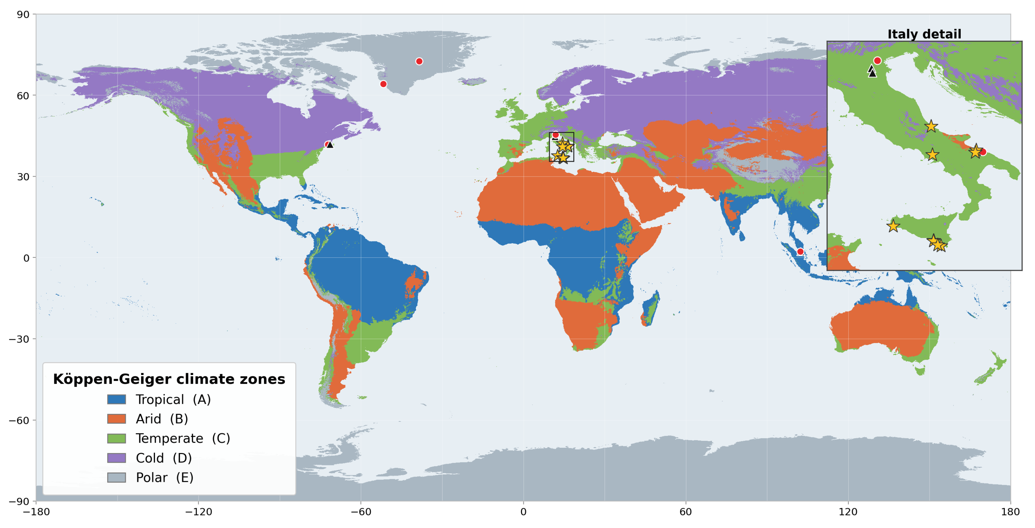
The analysis pipeline evaluates the predictive quality of the models by cross-referencing the extracted data with field measurements. The acquisition scripts run hourly queries to collect both the forecasts for the following hours and the current observation. Monitoring covers a total of 22 locations distributed across the five Köppen–Geiger macro-zones, as shown in Figure 2. The geographic selection follows a priority logic designed to maximise both data quality and climatic coverage. The highest priority was given to sites with directly available on-site physical measurements of solar irradiance, which in this study coincide with the Italian plants. Where such measurements were not available, preference was given to locations hosting large operational PV plants, identified via web search and verified on satellite imagery, so that the benchmark would remain anchored to sites of genuine energy-sector relevance. Finally, additional reference points were added by selecting, within each under-represented zone, the location of greatest human presence, which is also where surface meteorological reporting is most continuous and reliable; this is the case for the polar zone, represented by the largest Greenland settlement and a permanent inland research station.
A subsequent processing pipeline extracts, filters, aggregates, and processes the records from InfluxDB to compute Mean Bias Error (MBE), Mean Absolute Error (MAE), Symmetric Mean Absolute Percentage Error (sMAPE), coefficient of determination ( R 2 ), and 95% confidence intervals (CIs) for MAE and sMAPE. The confidence intervals were obtained by a block bootstrap [34] that preserves the serial dependence of the data. Each metric is written as the mean of its per-observation contributions over the time-by-site panel; contiguous temporal blocks of length L are then resampled with replacement, the metric is recomputed on each bootstrap panel, and the interval is read from the empirical percentiles of the resulting distribution and reported as a half-width. The block length is set to about three times the autocorrelation time of the error series, with a floor of 24 h so that each block spans at least one full diurnal cycle, and the intervals are computed at the 95 % level ( α = 0.05 ). This scheme accounts for the strong autocorrelation of the hourly records, which an interval based on independent observations would underestimate. Accordingly, two providers are regarded as differing significantly on a given variable when their confidence intervals do not overlap.
sMAPE [35,36] was selected for its scale-independence, enabling cross-location comparison regardless of microclimatic variations. However, the metric is sensitive to the absolute scale of the variable: for instance, atmospheric pressure oscillates around a mean of 1000 hPa, whereas temperature settles on seasonal means close to 15 °C (in non-extreme zones). Owing to this difference of almost two orders of magnitude, for the same absolute error the sMAPE of pressure is much smaller than that of temperature, making them non-comparable in relative terms. Additionally, sMAPE exhibits a known structural vulnerability to numerical instability when the values of the evaluated parameters approach zero, such as temperature regimes near 0 °C or irradiance during the dawn and dusk transitions, potentially amplifying minor absolute errors into large percentage distortions. To overcome these limitations, comparisons are strictly variable-by-variable, eliminating cross-variable scaling distortions. The aim is not to establish whether a given provider is more capable of recognising pressure than another is effective in forecasting temperature; the analysis focuses on the direct comparison between providers within the same physical quantity. By isolating the comparison per single variable, the distorting effect of scale is cancelled. Furthermore, to prevent near-zero instabilities from biasing the overall performance evaluation, the sMAPE-based rankings are systematically cross-checked against the MAE-based ones. Because MAE evaluates absolute physical deviations linearly, it remains unaffected by zero-value denominators, thereby providing a stable benchmark that confirms the robustness of the reported model hierarchies.
Data integrity is maintained through a non-intrusive preprocessing workflow: null values, empty strings, and records outside the physical scale are removed. Isolated gaps are imputed via temporal interpolation (maximum 3 h window, requiring valid preceding and succeeding values) using Python Pandas. A rolling-average filter is applied solely for plot readability, leaving statistical computations unchanged. The entire pipeline is fully reproducible from the archived database.
A final clarification concerns the irradiance reference: ground-truth PoA irradiance corresponds to physical on-site sensor measurements, while forecast PoA values are reconstructed from shortwave, diffuse, and direct normal components following [21].

4. Results

To evaluate the specific performance of each provider, a variable-by-variable analysis was conducted, where the comparison was naturally tailored to encompass only the subset of providers offering that specific variable. As detailed in Table 3, this approach allows to isolate the providers’ performance for each quantity. Observing the sMAPE and R 2 values, it clearly emerges that Provider-1 and Provider-3 represent the excellence of the sample, obtaining on average more solid and reliable results than the other providers, albeit with different specialisations. While Provider-1 is the most balanced across the entire spectrum of variables, Provider-3 shows very-high-profile performance in the categories in which it operates.
Wind speed behaves very differently and rewards no single provider. It is a disturbing factor across the board, with uniformly high sMAPE values, and the aggregate figures are close: on the R 2 , Provider-4 leads (0.42004), narrowly ahead of Provider-1 (0.37800) and Provider-3 (0.37353), with Provider-2 far behind (0.09946); on sMAPE the order is almost reversed, Provider-1 being the most accurate (54.77%) and Provider-3 the least (57.80%). As the disaggregated analysis below shows, these close aggregate values conceal markedly different behaviours.
As for sea-level pressure, while noting the specific excellence of Provider-4 (sMAPE 0.09584 and R 2 0.96280), Provider-1 remains extremely competitive ( R 2 0.91845), confirming its reliability even where it does not hold the absolute primacy. Humidity, in turn, confirms the supremacy of Provider-1 as a generalist model, with the lowest MAE, the highest R 2 and the lowest sMAPE. On cloud cover, the two providers are almost tied on MAE (≈30.3 against ≈30.4), and Provider-1 even carries the larger positive bias (MBE 15.27050 against 13.28663), so its advantage there rests on the relative error alone (sMAPE 76.53% against 84.49%).
Finally, the precipitation datum, analysed for Provider-1 only, highlights the intrinsic criticality of this variable. The negative R 2 value of 0.33895 suggests poor predictive capability, plausibly linked to the intermittent nature of precipitation and the possible mistimed placement of rainfall events.
In summary, this part of the analysis confirms that Provider-1 and Provider-3 sit on a superior performance plane, both significantly outdistancing Provider-2 and Provider-4 in consistency and precision.
To deepen what emerged from the aggregate analysis, the following subsections present a detailed examination per single meteorological variable. This step is fundamental to understanding not only the magnitude of the error (already discussed quantitatively), but also its dynamic nature and the capacity of the different models to follow the temporal fluctuations of the observed phenomena. For the graphical presentation only, a smoothing procedure based on a 14-day moving average was applied to maximise the readability of the time series and to mitigate the impact of high-frequency stochastic noise; this isolates the “real” trend and synoptic variations.

4.1. Temperature

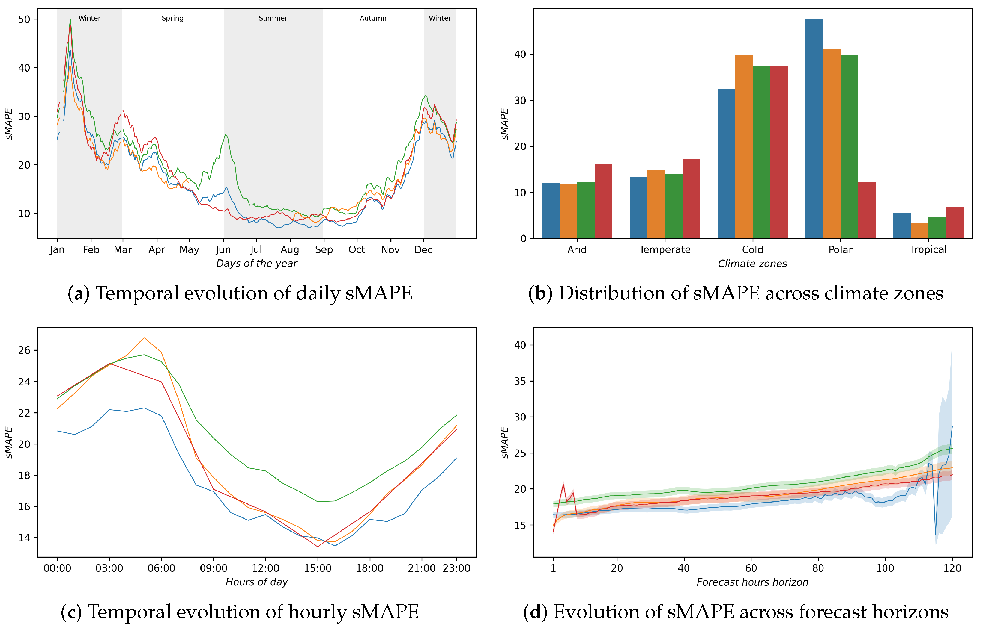
Ambient temperature is one of the most relevant meteorological variables for environmental monitoring and the energy transition, and it represents a particularly favourable case within meteorological modelling. Being an extremely sensitive quantity for many strategic sectors, providers invest a significant share of their predictive capacity in its optimisation, which is reflected in overall superior performance. Figure 3 shows the behaviour of the sMAPE computed on the temperature forecasts of the four analysed providers.
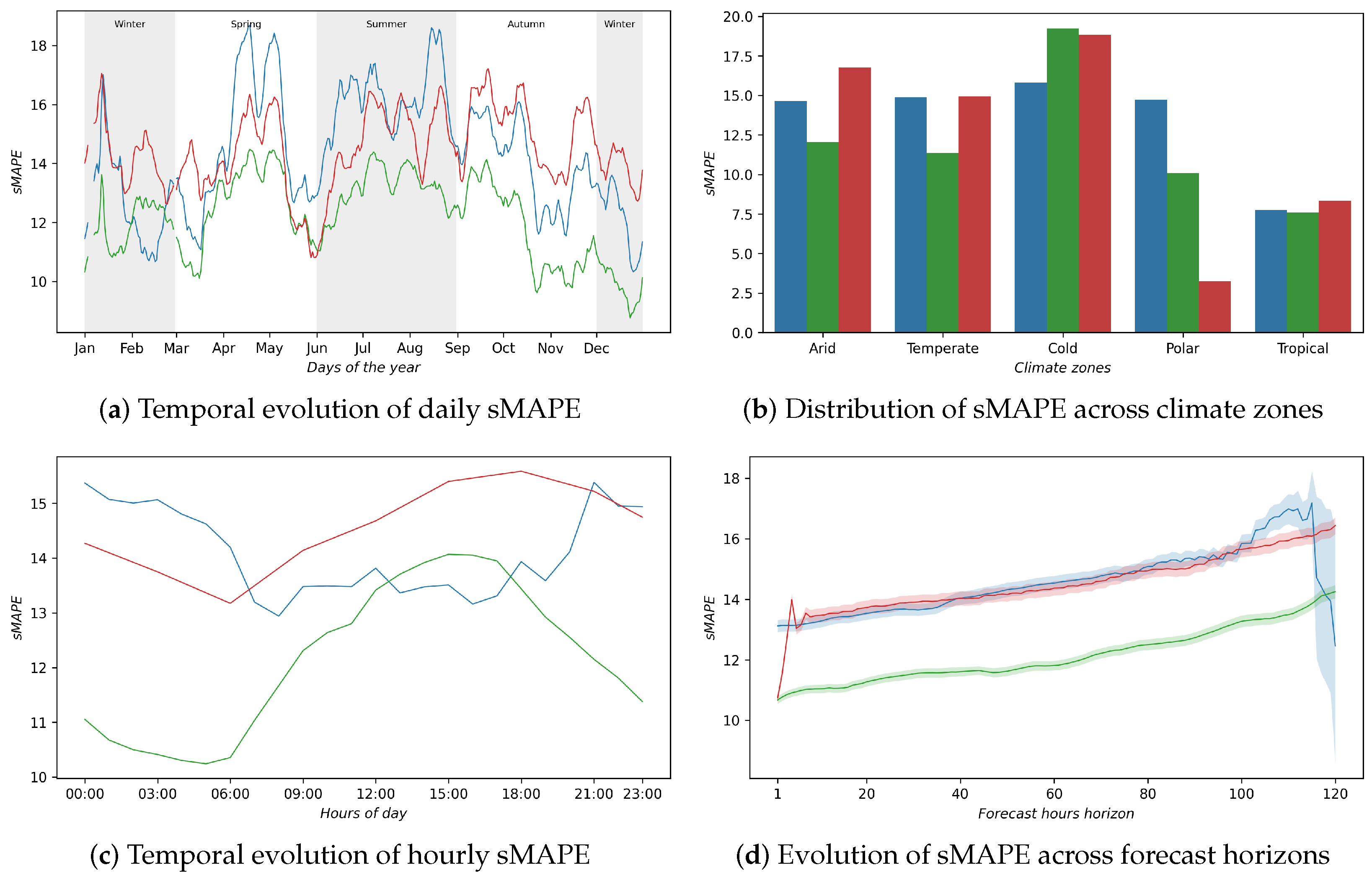
Overall, Provider-4 (blue) delivers the best performance, closely followed by Provider-2 (red) and Provider-3 (orange); Provider-1 (green) sits at the highest error values, while Provider-4 is the most exposed in the polar zone and at the long forecast horizon. The error is inversely correlated with ambient temperature: all providers exhibit lower sMAPE in the summer months (Figure 3a), in the warmer climate zones (Figure 3b, tropical and arid), and in the central hours of the day (Figure 3c), while the error peaks concentrate in the winter months, in the Cold and polar zones, and in the night hours. With respect to the forecast horizon (Figure 3d), Provider-1, Provider-2, and Provider-3 demonstrate a contained and quasi-linear error accumulation up to 120 h. Within the first 3 h, Provider-2 and Provider-3 register the lowest initial sMAPE values; however, Provider-2 undergoes prominent localised error spikes before stabilising after hour 6. Interestingly, Provider-4 consistently maintains the lowest systematic error across most of the forecast horizon; however, as it approaches the 120 h mark, it exhibits highly unstable behaviour, characterised by a sharp fluctuation in sMAPE and an explosion of variance.

4.2. Wind Speed

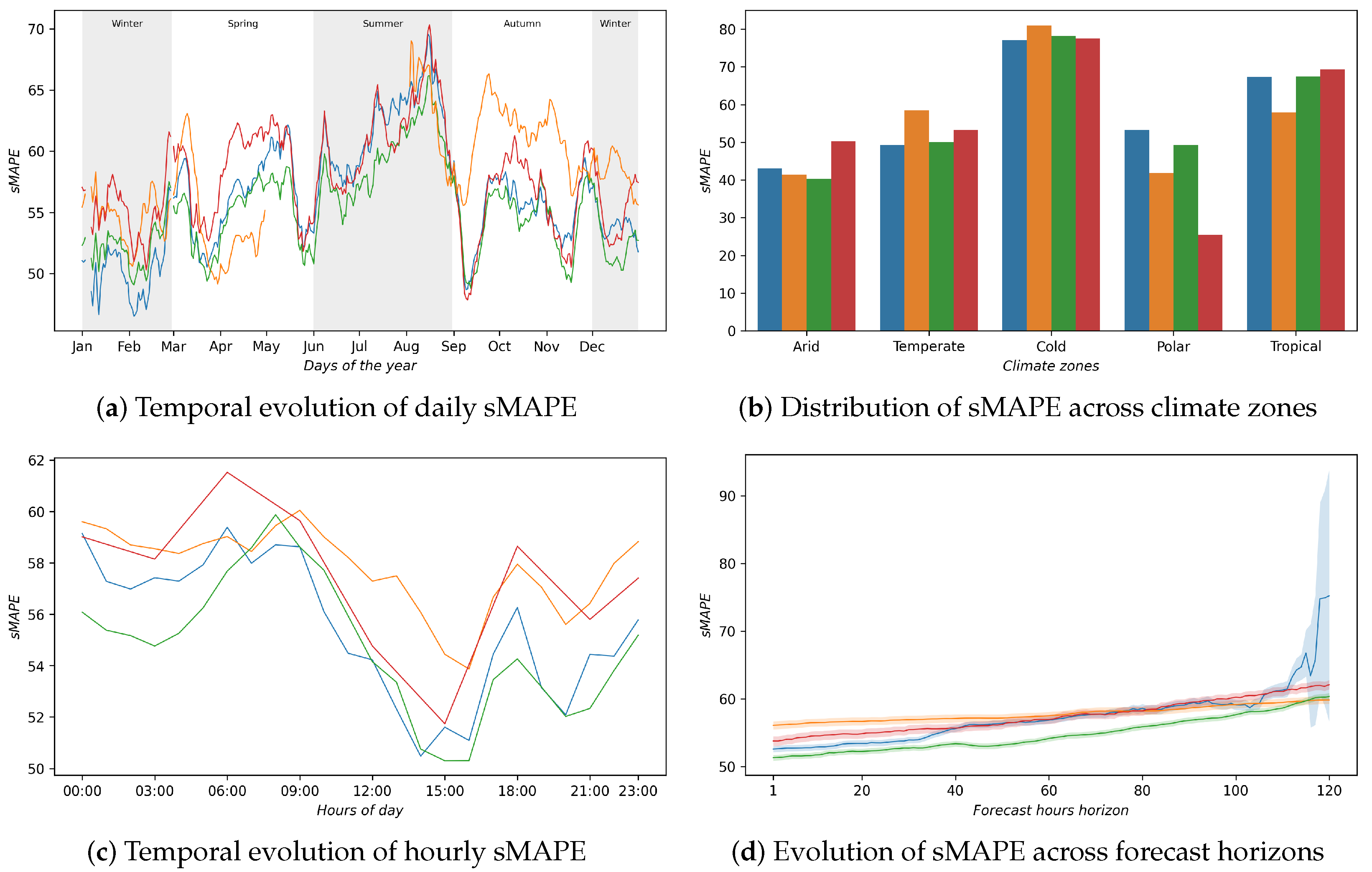
Overall, wind speed confirms itself as a variable of high forecasting complexity, characterised by low R 2 coefficients and decidedly high global sMAPE (Table 3). In this context, Provider-1 offers the lowest aggregate sMAPE (54.77%) and the steadiest behaviour, while Provider-4 attains the best aggregate R 2 (0.42004) and MAE; on the relative error, Provider-3 and Provider-2 trail. The disaggregated analysis, however, reveals strong structural fragilities concealed by these aggregate figures, particularly for Provider-3. The temporal analysis reveals strong annual variability (Figure 4a), from which only the stability of Provider-1 stands out, and a clear diurnal pattern common to all models (Figure 4c): the error reaches its minima in the afternoon, favoured by the greater predictability of solar atmospheric convection, and rises to its maxima at night and at dawn, when local dynamics and more complex synoptic flows come into play. In this morning transition phase, Provider-3 records the greatest criticality.
On the climatic plane (Figure 4b), Provider-1 dominates the temperate and cold zones. In cold climates Provider-3 records the highest sMAPE of the whole sample, while partly compensating with the best performance in the arid zone. With respect to the forecast horizon (Figure 4d), Provider-1 shows a slow and controlled degradation, while Provider-4 suffers a clear collapse of performance beyond 100 h, accompanied by a strong expansion of variance.

4.3. Humidity

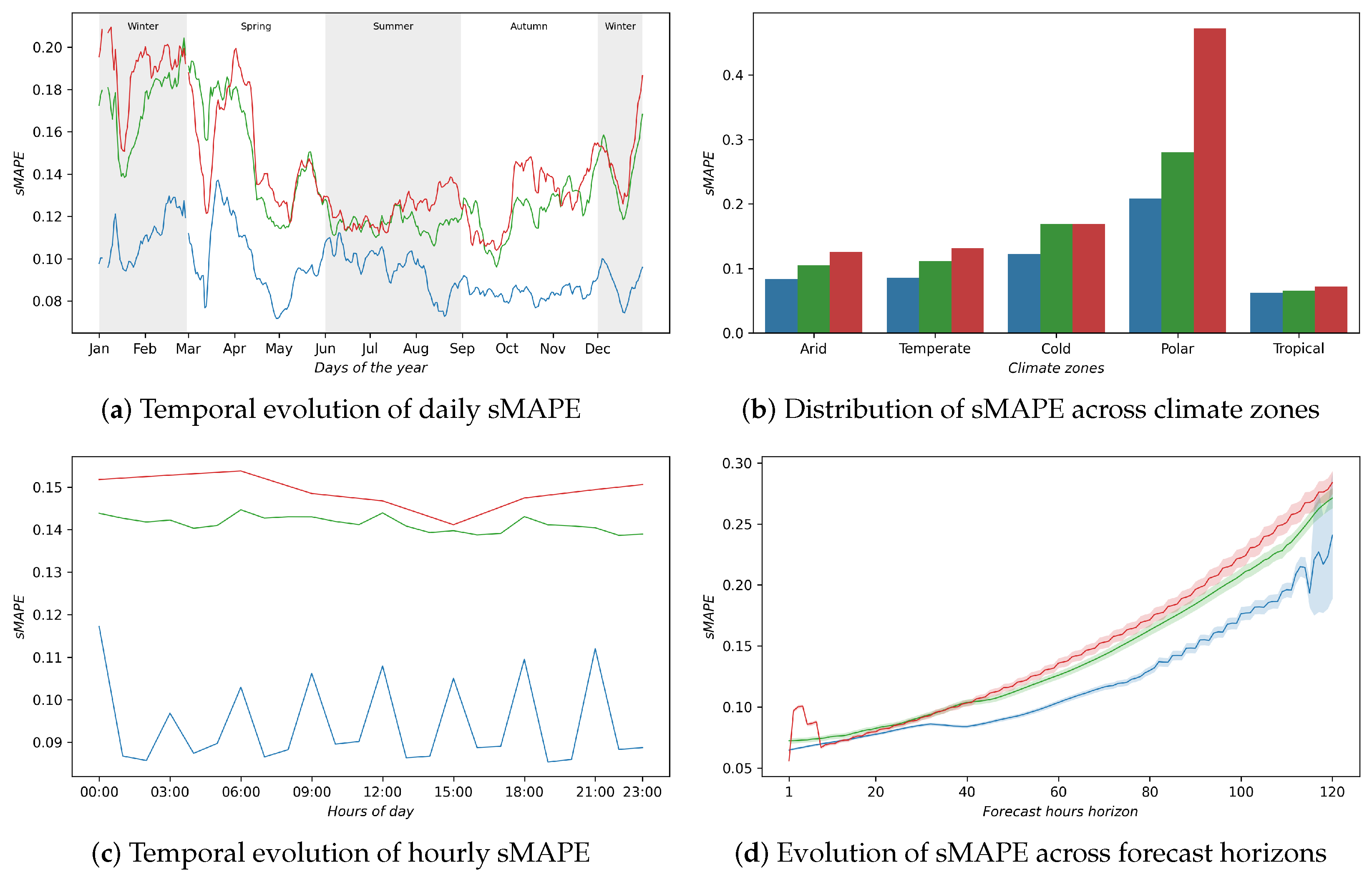
Overall, Provider-1 provides the best performance across almost all dimensions. Although Provider-4 retains a slight edge over Provider-2 on the aggregate metrics, in the disaggregated view it is the more penalised of the two, trailing Provider-2 across most climate zones and at the long forecast horizon. Provider-3 is not available for this variable. The error is more contained in the winter months and at night, while the peaks concentrate in spring-summer (Figure 5a) and in the central hours of the day (Figure 5c). Provider-4 is an exception, showing a different intraday cycle, higher error at night and lower in the central hours, with an evening peak around 21:00 that interrupts the expected decreasing trend. In autumn–winter the gap between providers widens: Provider-1 descends markedly towards its own absolute minima, while Provider-2 and Provider-4 remain at higher levels.
By climate zone (Figure 5b), Provider-1 and Provider-2 obtain the best performance in polar and tropical zones; the worst are recorded in cold for all providers, and in temperate for Provider-4, which is the most penalised in almost all zones except tropical. With respect to the forecast horizon (Figure 5d), Provider-1 grows gradually and in a controlled manner over the whole 120 h span. Provider-4 instead shows a more marked growth with collapse and a clear explosion of variance beyond 100 h. Provider-2 starts from exceptionally low values at the first hour, rising abruptly within the first 3–5 h to settle at its stationary level.

4.4. Sea-Level Pressure

Sea-level pressure, shared by only three models (Provider-3 absent), represents the most favourable variable of the entire study. It is the only case in which Provider-4 emerges as the dominant solution over Provider-1 and Provider-2.
The temporal analysis shows that the error concentrates mainly in the winter and spring months (Figure 6a), the part of the year in which Provider-4 constantly maintains the lowest error profile against the greater variability and inadequacy of Provider-2. The hourly profile, however, introduces a strong structural anomaly for Provider-4 (Figure 6c): the model exhibits a systematic and regular oscillation every two hours throughout the day, lacking physical coherence and linked to a probable defect of the forecasting system. By contrast, Provider-1 and Provider-2 show flat and physically plausible behaviours, with Provider-1 stably more precise.
On a climatic basis (Figure 6b), Provider-4 proves slightly better across almost all zones, except the tropical one where the three competitors are equivalent. The polar climate confirms itself as the most challenging context for all models, while recording the most marked gaps between performances. With respect to the forecast horizon (Figure 6d), the error growth over 120 h remains linear and without sudden drops for all providers. If Provider-2 offers the best start in the very first hours, Provider-4 merely shows a greater expansion of the confidence interval beyond 100 h, without, however, compromising the overall robustness of the model.

4.5. Cloud Cover

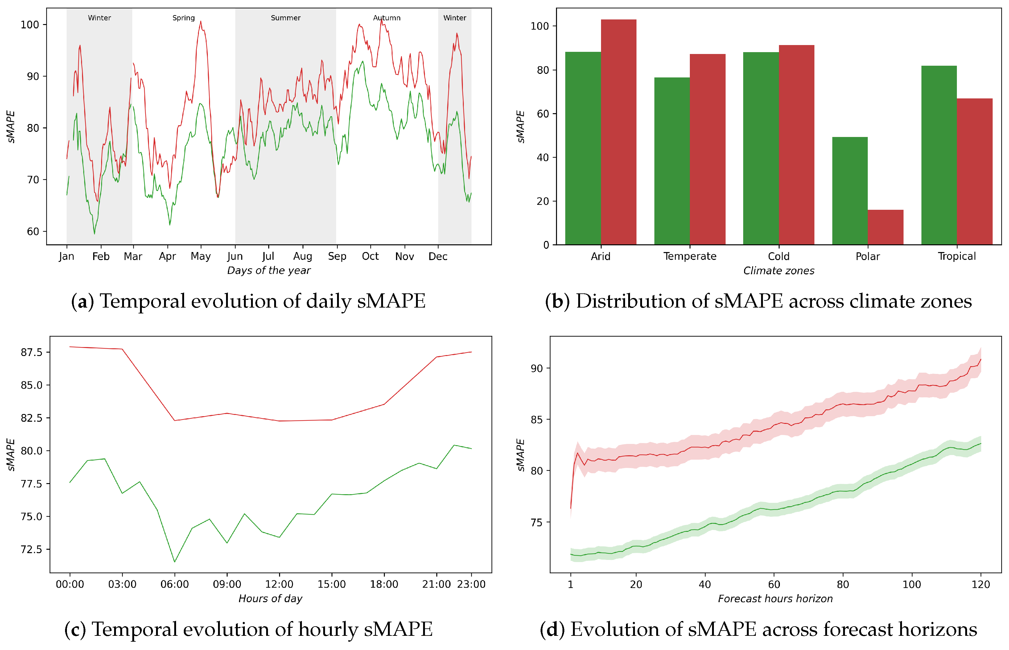
Cloud cover is the only variable of the sample shared by just two models (Provider-3 and Provider-4 absent), and it is configured as one of the most challenging quantities to predict because of its intrinsically discontinuous and stochastic nature. The temporal analysis highlights a clear seasonal pattern (Figure 7a): the error contracts in the winter and spring months and surges in the summer-autumn period. This dynamic reflects the nature of summer convective systems (local and short-lived), which are less predictable than winter stratiform cover. The hourly profiles show distinct trends (Figure 7c): while Provider-1 oscillates between day and night, reaching its lowest sMAPE values in the early morning around 06:00 before gradually rising, Provider-2 maintains a consistently higher error rate, characterised by a sharp decrease between 03:00 and 06:00 followed by a stable, linear recovery towards the late evening.
On a climatic basis (Figure 7b), the polar zone represents the region where both competitors achieve their respective local error minima, while simultaneously exhibiting the most pronounced performance discrepancy. Within the remaining climate zones, the two providers display substantially comparable trends; specifically, Provider-2 demonstrates a marginal advantage in the tropical zone, whereas Provider-1 prevails across the arid, temperate, and cold regions. With respect to the forecast horizon (Figure 7d), Provider-2 exhibits a sharp and sudden increase in error immediately after the first hour, where it briefly registers its lowest sMAPE value. Provider-1 consistently maintains significantly superior accuracy across the entire 120 h spectrum. In both cases error degradation proceeds in a stable, quasi-linear fashion without sudden collapses, preserving a constant performance gap until the final forecast step. Overall, the extremely low coefficients of determination confirm that cloud cover remains the most critical forecasting limit of the entire study.

4.6. Rain

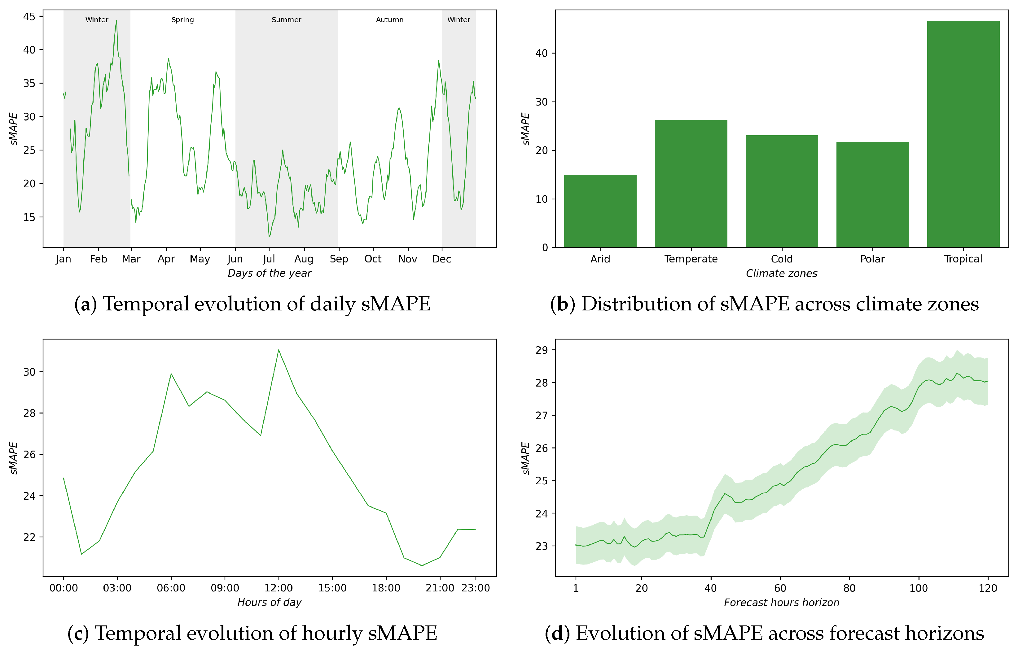
Rain constitutes the limiting case of the entire study, being the only variable predicted by a single model, Provider-1. The negative R 2 value formalises a clear modelling limit (Table 3), showing how the simulation performs worse than a trivial mean-based predictor because of the intermittent and sub-grid nature of precipitation [37]. The temporal analysis reveals a strong divergence between the seasonal and the hourly dimensions. The seasonal series (Figure 8a) is by far the most erratic of the study, devoid of structured trends and marked by violent oscillations even within the same months. By contrast, the hourly profile (Figure 8c) shows a solid pattern coherent with atmospheric physics: the error is minimal in the night hours, when spatially stable stratiform or frontal rainfall prevails, and peaks clearly at midday, in correspondence with the solar heating that activates locally and intrinsically unpredictable convective cells.
On a climatic basis (Figure 8b), geographical differentiation markedly affects accuracy. The model obtains the best performance in the arid zone, while settling on intermediate and comparable values in the temperate, cold and polar zones. The maximum error is recorded in the tropical zone, where the dominance of deep convection generates short and intense phenomena, extremely complex to intercept for a global-scale model. With respect to the forecast horizon (Figure 8d), the error degradation over 120 h proceeds linearly, constantly and with stable variance. The absence of vertical drops or long-term anomalies reflects the fact that the forecast carries a structurally high uncertainty from the very first hours of simulation.

4.7. Plane-of-Array Irradiance

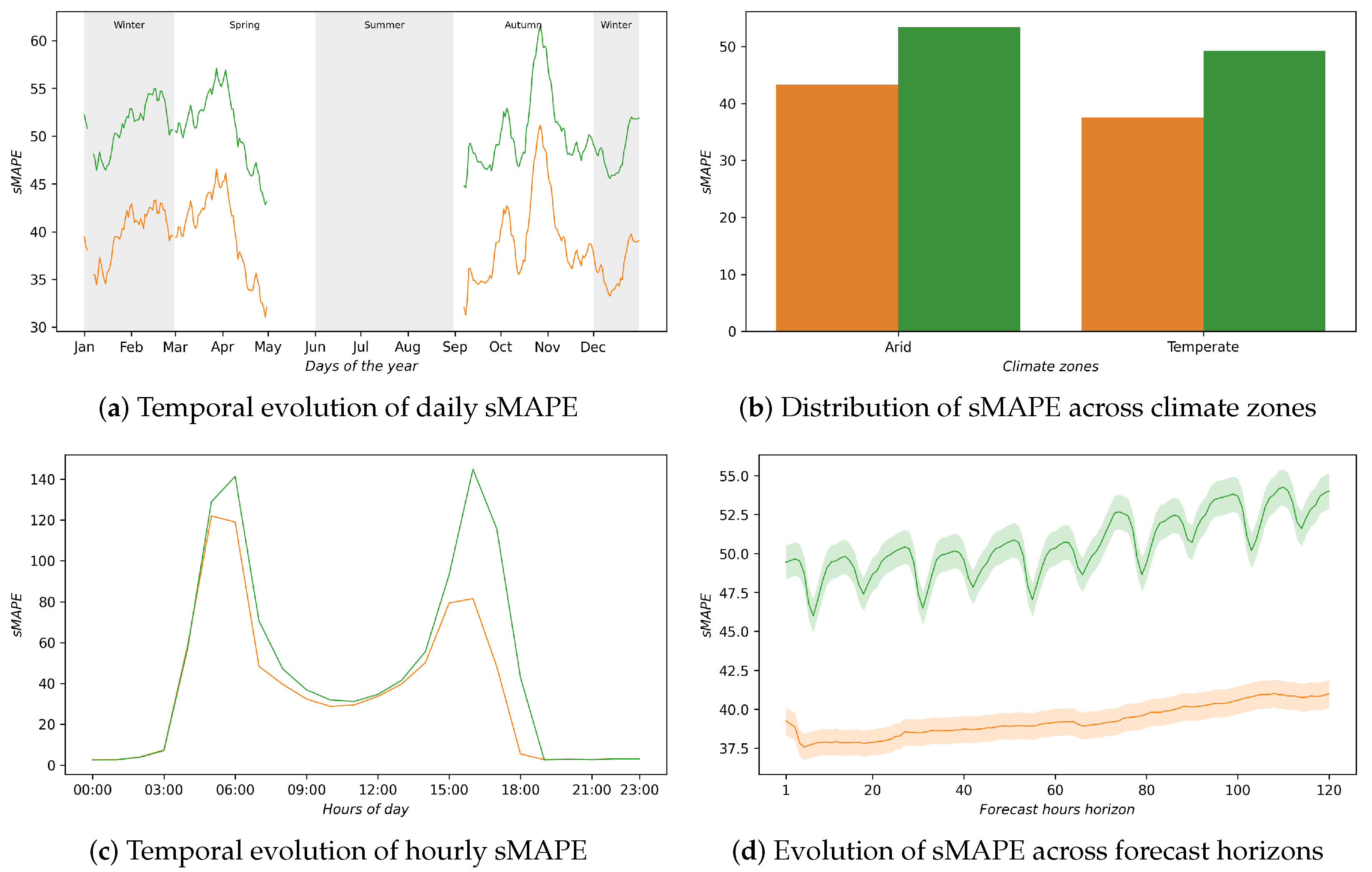
Irradiance on the plane of the modules is a variable shared by only two providers (Provider-2 and Provider-4 absent), with Provider-3 establishing itself as the dominant solution across all the analysed dimensions. The temporal analysis (Figure 9a) shows a seasonal behaviour in which errors tend to be more contained in the second part of the year, then growing in the winter–spring period. Notably, the best performance is observed in late spring and in autumn, with the gap between providers more marked than in other periods, always in favour of Provider-3, which is systematically better throughout the whole year.
By climate zone (Figure 9b), the availability of ground stations is limited to only two zones, arid and temperate. Provider-3 prevails in both, with the temperate zone configured as the slightly more favourable context for both models. The intraday profile (Figure 9c) is, by physical definition, restricted to daylight hours (about 04:00–18:00), with null values at night. The greatest predictive difficulties concentrate in the dawn-dusk transition bands, where irradiance is close to zero. The shared minimum lies between 10:00 and 12:00, corresponding with the hours of maximum irradiance, which are physically more stable and parametrisable. At the end of the day a structural difference emerges: Provider-3 zeroes its sMAPE around 18:00, showing the capacity to correctly predict the extinction of the solar signal before sunset, while Provider-1 shows a substantial growth, a symptom of an inability to model that zeroing. Provider-3 maintains lower errors throughout the daytime span. With respect to the forecast horizon (Figure 9d), no provider shows performance collapses. Provider-3 presents a slow, almost linear degradation, free of anomalies over all 120 h, with a narrow confidence interval attesting to its stability. Provider-1 instead shows an oscillatory pattern with regular periodicity, remaining at systematically higher sMAPE values.

5. Discussion

The analysis of the results outlines a clear hierarchy of predictability linked to the physical complexity of the variables. Sea-level pressure sits at the apex of stability, governed by slow, well-parametrised large-scale synoptic dynamics. Temperature follows, a continuous variable strongly constrained by radiative thermal cycles, while relative humidity occupies an intermediate position, where the correlation with temperature is partially disturbed by evapotranspiration fluxes and local convection. Wind introduces a critical discontinuity owing to microclimatic variability. PoA occupies an intermediate position: a still-appreciable sMAPE (≈39–51%), driven by the sub-grid cloud component, coexists with a markedly higher R 2 (0.75–0.82) thanks to the deterministic component of solar geometry, which confers a well-defined and parametrisable diurnal structure on the variable. Finally, cloud cover and rain confirm themselves as variables structurally refractory to global modelling because of their asymmetric and intermittent nature, with rain recording a negative R 2 , performing worse than a mean-based predictor.

5.1. Comparative Characterisation of the Providers

The relative evaluation of the providers outlines complex performance geometries, identifying generalist solutions and elite specialisations.
Provider-1 is the reference benchmark of the study. While not holding the absolute primacy in every single scenario, it demonstrates a unique robustness and cross-cutting consistency across the entire spectrum of variables and dimensions analysed. It is the most balanced model and the only provider to cover all six meteorological variables (including rain) and irradiance. For multi-variable operational applications over horizons up to 5 days, it represents the safest and most reliable choice.
Provider-3 shows the typical profile of the “elite specialist”. Available for temperature, wind speed and irradiance, it offers very-high-profile performance in the contexts in which it operates, establishing itself as the dominant solution on PoA irradiance (Table 3). Its excellence is therefore selective rather than uniform: on wind its aggregate accuracy is already among the weakest of the sample, and the disaggregation exposes a strong geographical heterogeneity, with the cold-zone sMAPE (>70%) far exceeding the aggregate value (≈58%). This highlights an important methodological warning that aggregate figures can conceal both spatial heterogeneity within a variable and quality contrasts between variables.
Provider-2 settles at an intermediate level. A recurring characteristic is its anomalous behaviour in the very first forecast hours for humidity, wind and cloud cover, where it exhibits exceptionally low sMAPE that rise abruptly within the first hours of prediction. This pattern indicates a strong recent-data assimilation mechanism, which confers a real operational advantage exclusively in very-short-term nowcasting.
Provider-4 is the most paradoxical profile of the study. On the variables it covers it is frequently the most accurate in aggregate terms, attaining the best sMAPE and MAE on temperature, the best R 2 and MAE on wind, and the clearest dominance on pressure ( R 2 = 0.96280). Yet two structural defects limit its general operational use: a systematic performance collapse beyond 100 h, with an explosion of variance for temperature, wind and humidity, and a physically incoherent oscillation of the pressure error every two hours throughout the day. Combined with the narrowest variable coverage of the sample (no cloud cover, rain or irradiance), these defects make it a strong short-horizon choice on its supported variables rather than a reliable general-purpose solution.

5.2. Cross-Cutting Patterns: Seasonality, Climate Zone, Diurnal Cycle and Forecast Horizon

The multidimensional disaggregation highlights behavioural signatures linked to physical forcings and to the architectural limits of the predictive models.
Seasonality and climate zones—Two opposite seasonal dynamics emerge: temperature shows the maximum error in winter, whereas pressure shows the minimum error in summer, linked to winter cyclonic baric variability. Conversely, humidity and cloud cover see the error surge in summer and autumn due to the convective, cumuliform, and local nature of warm phenomena. Geographically, the polar zone amplifies the gaps between providers for temperature and generates the highest sMAPE for pressure, while the minimum error for rain is recorded in the arid zone. The tropical zone instead represents the maximum challenge for rain because of the dominance of sub-grid deep convection, while offering a favourable scenario for pressure and temperature thanks to their thermodynamic stability at such latitudes. Irradiance, available only for the arid and temperate zones, is slightly more accurate in the temperate zone for both providers.
Diurnal cycle—The intraday profiles reflect precise thermodynamic responses: temperature and wind show minimum error in the afternoon and maximum at night, while humidity and rain peak in the central hours, driven by diurnal evapotranspiration and convective triggering, respectively. Irradiance, constrained by definition to daylight hours, is least accurate at the dawn-dusk transitions and most accurate between 10:00 and 12:00; only Provider-3 correctly captures the signal’s extinction near 18:00, while Provider-1 shows a substantial growth of the error.
Forecast horizon—Degradation follows two patterns: a slow, near-linear growth in error for pressure, rain, and Provider-3 irradiance. For rain, this reflects a persistently high uncertainty from the first hours rather than genuine stability. A sharp performance collapse of Provider-4 is observed beyond 100 h for temperature, wind and humidity, a recurrence across independent variables that suggests a structural limit in its numerical-integration architecture or in the management of the boundaries of its predictive window.

6. Conclusions

This study proposed and applied a reproducible, dual-source framework for the comparative evaluation of weather and solar irradiance forecast providers, validated throughout against independent references rather than against the providers’ own model-derived observation products: real surface-station observations for the atmospheric variables and on-site sensors at operational PV plants for irradiance. The variable-by-variable analysis established a clear hierarchy of predictability (from the highly stable sea-level pressure to the structurally refractory cloud cover and rain) and showed that aggregate metrics alone can be misleading when marked spatial or seasonal heterogeneity is present. Among the surveyed services, one generalist provider emerged as the most balanced and reliable choice for multi-variable operational monitoring up to 5 days, while a second proved to be an elite specialist, dominant on PoA irradiance. For the energy operator, the value lies not in a fixed ranking of named services but in a transferable procedure: applying the proposed framework to the providers available for a given asset yields the selection criteria (by variable, forecast horizon and climatic context) needed to reduce the financial and operational risks associated with forecast uncertainty. Future work will extend the geographical coverage of the ground-truth irradiance measurements in both number of instrumented sites and spatial extent, broaden the set of providers and variables evaluated, and connect the observed forecast errors to their operational and economic consequences for grid balancing.

Author Contributions

Conceptualization, G.S. and G.P.; methodology, G.S. and G.P.; software, G.S.; validation, G.S., G.P. and S.D.; formal analysis, G.S. and G.P.; investigation, G.S. and S.D.; resources, S.D.V. and G.D.F.; data curation, G.S. and G.P.; writing (original draft preparation), G.S., S.D. and G.P.; writing (review and editing), G.P., S.D., S.D.V. and G.D.F.; visualization, G.S., S.D. and G.P.; supervision, G.P. and G.D.F.; project administration, G.D.F.; funding acquisition, G.D.F. All authors have read and agreed to the published version of the manuscript.

Funding

This research received no external funding.

Data Availability Statement

The reference datasets used for validation are publicly available: surface observations (NOAA Integrated Surface Database) via Meteostat (https://meteostat.net accessed on 16 June 2026) and the ERA5 reanalysis via the Copernicus Climate Data Store (https://cds.climate.copernicus.eu accessed on 16 June 2026). The providers’ forecasts were retrieved from their public and commercial APIs and are reproducible by querying the same endpoints; they are not redistributed here in accordance with the providers’ terms of use. The on-site PoA irradiance is proprietary to the plant owners and subject to non-disclosure agreements; it can be made available on reasonable request to the corresponding author, subject to the owners’ authorisation.

Conflicts of Interest

The authors declare no conflicts of interest.

Abbreviations

The following abbreviations are used in this manuscript:
DNIDirect Normal Irradiance
DHIDiffuse Horizontal Irradiance
GHIGlobal Horizontal Irradiance
PoAPlane of Array
VREVariable Renewable Energy
MAEMean Absolute Error
MBEMean Bias Error
sMAPESymmetric Mean Absolute Percentage Error
R 2 Coefficient of Determination
IFSIntegrated Forecasting System (ECMWF)
GFSGlobal Forecast System (NOAA/NCEP)
AIFSArtificial Intelligence Forecasting System (ECMWF)
NWPNumerical Weather Prediction
APIApplication Programming Interface
DEMDigital Elevation Model
STCStandard Test Conditions

References

  1. IPCC. Climate Change 2023: Synthesis Report. Contribution of Working Groups I, II and III to the Sixth Assessment Report of the Intergovernmental Panel on Climate Change; Technical report; IPCC: Geneva, Switzerland, 2023. [Google Scholar] [CrossRef] [Scilit]
  2. Correljé, A.; van der Linde, C. Energy supply security and geopolitics: A European perspective. Energy Policy 2006, 34, 532–543. [Google Scholar] [CrossRef] [Scilit]
  3. Hartvig, Á.; Kiss-Dobronyi, B.; Kotek, P.; Tóth, B.; Gutzianas, I.; Zareczky, A. The economic and energy security implications of the Russian energy weapon. Energy 2024, 294, 130972. [Google Scholar] [CrossRef] [Scilit]
  4. Szulecki, K.; Overland, I. Russian nuclear energy diplomacy and its implications for energy security in the context of the war in Ukraine. Nat. Energy 2023, 8, 413–421. [Google Scholar] [CrossRef] [Scilit]
  5. Caldara, D.; Iacoviello, M. Measuring Geopolitical Risk. Am. Econ. Rev. 2022, 112, 1194–1225. [Google Scholar] [CrossRef] [Scilit]
  6. Lin, F.; Li, X.; Jia, N.; Feng, F.; Huang, H.; Huang, J.; Fan, S.; Ciais, P.; Song, X. The impact of Russia-Ukraine conflict on global food security. Glob. Food Secur. 2023, 36, 100661. [Google Scholar] [CrossRef] [Scilit]
  7. Wu, Y.; Song, P.; Lin, S.; Peng, L.; Li, Y.; Deng, Y.; Deng, X.; Lou, W.; Yang, S.; Zheng, Y.; et al. Global Burden of Respiratory Diseases Attributable to Ambient Particulate Matter Pollution: Findings From the Global Burden of Disease Study 2019. Front. Public Health 2021, 9, 740800. [Google Scholar] [CrossRef] [Scilit] [PubMed]
  8. Borggrefe, F.; Neuhoff, K. Balancing and Intraday Market Design: Options for Wind Integration; SSRN Scholarly Paper 1945724; Social Science Research Network: Rochester, NY, USA, 2011. [Google Scholar]
  9. Chatuanramtharnghaka, B.; Deb, S.; Singh, K.R.; Ustun, T.S.; Kalam, A. Reviewing Demand Response for Energy Management with Consideration of Renewable Energy Sources and Electric Vehicles. World Electr. Veh. J. 2024, 15, 412. [Google Scholar] [CrossRef] [Scilit]
  10. Muqtadir, A.; Li, B.; Qi, B.; Ge, L.; Du, N.; Lin, C. Demand Response Potential Forecasting: A Systematic Review of Methods, Challenges, and Future Directions. Energies 2025, 18, 5217. [Google Scholar] [CrossRef] [Scilit]
  11. Apata, O.; Munda, J.L.; Migabo, E.M. Artificial Intelligence for Predictive Maintenance and Performance Optimization in Renewable Energy Systems: A Comprehensive Review. Energies 2026, 19, 536. [Google Scholar] [CrossRef] [Scilit]
  12. Jiao, X.; Xiao, W. Review of Data-Driven Approaches Applied to Time-Series Solar Irradiance Forecasting for Future Energy Networks. Energies 2025, 18, 5823. [Google Scholar] [CrossRef] [Scilit]
  13. Antonanzas, J.; Osorio, N.; Escobar, R.; Urraca, R.; Martinez-de Pison, F.; Antonanzas-Torres, F. Review of photovoltaic power forecasting. Sol. Energy 2016, 136, 78–111. [Google Scholar] [CrossRef] [Scilit]
  14. Wang, H.; Lei, Z.; Zhang, X.; Zhou, B.; Peng, J. A review of deep learning for renewable energy forecasting. Energy Convers. Manag. 2019, 198, 111799. [Google Scholar] [CrossRef] [Scilit]
  15. Sgueglia, A.; Spinelli, G.; Visaggio, C.; De Vito, S.; Di Francia, G. False Data Injection Identification in Energy Microgrids Through an Anomaly Detection Approach. In Proceedings of the AISEM Annual Conference on Sensors and Microsystems; Springer: Cham, Switzerland, 2025; pp. 387–392. [Google Scholar]
  16. Kaur, A.; Nonnenmacher, L.; Pedro, H.; Coimbra, C. Benefits of solar forecasting for energy imbalance markets. Renew. Energy 2016, 86, 819–830. [Google Scholar] [CrossRef] [Scilit]
  17. Kraas, B.; Schroedter-Homscheidt, M.; Madlener, R. Economic merits of a state-of-the-art concentrating solar power forecasting system for participation in the Spanish electricity market. Sol. Energy 2013, 93, 244–255. [Google Scholar] [CrossRef] [Scilit]
  18. Sun, Q.; Li, X.; Zhao, J.; Zhu, J.; Wu, Z.; Gao, T.; Yuan, Y. Joint planning of transportable and flexible resources in distribution systems for renewable integration and resilience enhancement. Sustain. Energy Grids Netw. 2026, 46, 102292. [Google Scholar] [CrossRef] [Scilit]
  19. Kasimalla, S.R.; Park, K.; Zaboli, A.; Hong, Y.; Choi, S.L.; Hong, J. An Evaluation of Sustainable Power System Resilience in the Face of Severe Weather Conditions and Climate Changes: A Comprehensive Review of Current Advances. Sustainability 2024, 16, 3047. [Google Scholar] [CrossRef] [Scilit]
  20. Notton, G.; Nivet, M.; Voyant, C.; Paoli, C.; Darras, C.; Motte, F.; Fouilloy, A. Intermittent and stochastic character of renewable energy sources: Consequences, cost of intermittence and benefit of forecasting. Renew. Sustain. Energy Rev. 2018, 87, 96–105. [Google Scholar] [CrossRef] [Scilit]
  21. Piantadosi, G.; Dutto, S.; Galli, A.; De Vito, S.; Sansone, C.; Di Francia, G. Photovoltaic power forecasting: A Transformer based framework. Energy AI 2024, 18, 100444. [Google Scholar] [CrossRef] [Scilit]
  22. Voyant, C.; Notton, G.; Kalogirou, S.; Nivet, M.; Paoli, C.; Motte, F.; Fouilloy, A. Machine learning methods for solar radiation forecasting: A review. Renew. Energy 2017, 105, 569–582. [Google Scholar] [CrossRef] [Scilit]
  23. Hersbach, H.; Bell, B.; Berrisford, P.; Hirahara, S.; Horányi, A.; Muñoz-Sabater, J.; Nicolas, J.; Peubey, C.; Radu, R.; Schepers, D.; et al. The ERA5 global reanalysis. Q. J. R. Meteorol. Soc. 2020, 146, 1999–2049. [Google Scholar] [CrossRef] [Scilit]
  24. Bauer, P.; Thorpe, A.; Brunet, G. The quiet revolution of numerical weather prediction. Nature 2015, 525, 47–55. [Google Scholar] [CrossRef] [Scilit] [PubMed]
  25. Lang, S.; Alexe, M.; Chantry, M.; Dramsch, J.; Pinault, F.; Raoult, B.; Clare, M.; Lessig, C.; Maier-Gerber, M.; Magnusson, L.; et al. AIFS–ECMWF’s data-driven forecasting system. arXiv 2024, arXiv:2406.01465. [Google Scholar] [CrossRef] [Scilit]
  26. Smith, A.; Lott, N.; Vose, R. The Integrated Surface Database: Recent Developments and Partnerships. Bull. Am. Meteorol. Soc. 2011, 92, 704–708. [Google Scholar] [CrossRef] [Scilit]
  27. Meteostat. Meteostat: Open Hourly and Daily Weather Data. Available online: https://meteostat.net (accessed on 16 June 2026).
  28. Sengupta, M.; Habte, A.; Wilbert, S.; Gueymard, C.; Remund, J.; Lorenz, E.; van Sark, W.; Jensen, A. Best Practices Handbook for the Collection and Use of Solar Resource Data for Solar Energy Applications, 4th ed.; Technical report nrel/tp-5d00-88300; National Renewable Energy Laboratory: Golden, CO, USA, 2024. [Google Scholar] [CrossRef] [Scilit]
  29. Skoplaki, E.; Palyvos, J. On the temperature dependence of photovoltaic module electrical performance: A review of efficiency/power correlations. Sol. Energy 2009, 83, 614–624. [Google Scholar] [CrossRef] [Scilit]
  30. IEC 61215-1:2021; Terrestrial Photovoltaic (PV) Modules—Design Qualification and Type Approval—Part 1: Test Requirements. International Electrotechnical Commission (IEC): Geneva, Switzerland, 2021.
  31. IEC 61646:2008; Thin-Film Terrestrial Photovoltaic (PV) Modules–Design Qualification and Type Approval. International Electrotechnical Commission (IEC): Geneva, Switzerland, 2008.
  32. UL 1703; UL Standard for Safety for Flat-Plate Photovoltaic Modules and Panels. Underwriters Laboratories Inc. (UL): Northbrook, IL, USA, 2004.
  33. Beck, H.E.; McVicar, T.R.; Vergopolan, N.; Berg, A.; Lutsko, N.J.; Dufour, A.; Zeng, Z.; Jiang, X.; van Dijk, A.I.J.M.; Miralles, D.G. High-resolution (1 km) Köppen-Geiger maps for 1901–2099 based on constrained CMIP6 projections. Sci. Data 2023, 10, 724. [Google Scholar] [CrossRef] [Scilit] [PubMed]
  34. Künsch, H.R. The Jackknife and the Bootstrap for General Stationary Observations. Ann. Stat. 1989, 17, 1217–1241. [Google Scholar] [CrossRef] [Scilit]
  35. Makridakis, S. Accuracy measures: Theoretical and practical concerns. Int. J. Forecast. 1993, 9, 527–529. [Google Scholar] [CrossRef] [Scilit]
  36. Hyndman, R.; Koehler, A. Another look at measures of forecast accuracy. Int. J. Forecast. 2006, 22, 679–688. [Google Scholar] [CrossRef] [Scilit]
  37. Arakawa, A. The cumulus parameterization problem: Past, present, and future. J. Clim. 2004, 17, 2493–2525. [Google Scholar] [CrossRef]
Figure 1. Daily mean day-ahead irradiance forecast error versus daily mean imbalance of the Southern Italian bidding zone, over daylight hours between March 2025 and April 2026; the day-ahead irradiance forecast is benchmarked against on-site PoA measurements at the instrumented plants, while the imbalance is the aggregate value settled by the national transmission system operator. Solid lines are per-provider linear fits; each marker is a daily mean for one provider.
Energies 19 03361 g001
Figure 2. Evaluation and measurement sites overlaid on the Köppen–Geiger climate classification (1991–2020 normals) [33]. Marker shape denotes the data available at each site: stars indicate sites with on-site PV (PoA irradiance) measurements; triangles indicate sites hosting an operational PV plant for which on-site measurements were not available; circles indicate the remaining reference locations. The inset details the Italian sites; markers may overlap where sites are geographically close. The figure is an original elaboration produced by the authors; the site markers, the Italian inset and the overall composition are our own work. The only third-party element is the underlying climate-zone raster (Beck et al., 2023, 1 km Köppen–Geiger, gloh2o.org) [33], which is distributed under the Creative Commons Attribution 4.0 (CC BY 4.0) license and is reproduced here with the required attribution.
Energies 19 03361 g002
Figure 3. Trend in sMAPE calculated from temperature measurements and forecasts. Provider-1 (green), Provider-2 (red), Provider-3 (orange), Provider-4 (blue).
Energies 19 03361 g003
Figure 4. Trend in sMAPE calculated from wind-speed measurements and forecasts. Provider-1 (green), Provider-2 (red), Provider-3 (orange), Provider-4 (blue).
Energies 19 03361 g004
Figure 5. Trend in sMAPE calculated from humidity measurements and forecasts. Provider-1 (green), Provider-2 (red), Provider-4 (blue).
Energies 19 03361 g005
Figure 6. Trend in sMAPE calculated from sea-level-pressure measurements and forecasts. Provider-1 (green), Provider-2 (red), Provider-4 (blue).
Energies 19 03361 g006
Figure 7. Trend in sMAPE calculated from cloud-cover measurements and forecasts. Provider-1 (green), Provider-2 (red).
Energies 19 03361 g007
Figure 8. Trend in sMAPE calculated from rain measurements and forecasts. Provider-1 (green).
Energies 19 03361 g008
Figure 9. Trend in sMAPE calculated from PoA-irradiance measurements and forecasts. Provider-1 (green), Provider-3 (orange).
Energies 19 03361 g009
Table 1. Synoptic overview of the surveyed weather-data providers and their delivery characteristics. Y/N denote availability of the weather and solar irradiance forecast.
ProviderWeatherIrrad. aHorizonModel Selection bAccess
AccuWeatherY cY c120 h/15 dn.d.API, web
MeteoAMYN3–5 dmulti-model ensembleAPI, web
MeteoblueYY14 down + multi-model ensembleAPI, web
MeteosourceYY7 d/30 dmulti-model ensembleAPI
Open-MeteoYY16 d/3–6 moown + third party user-selectableAPI
OpenWeatherYY c4–16 dn.d.API, web
Tomorrow.ioYY c120 h/5 dmulti-model ensembleAPI, app, web
Visual CrossingYY c15 dmulti-model ensembleAPI
Weather APIYY c14 dmulti-model ensemble with ML and weather stationAPI
WeatherBitY cY c16 dmulti-model ensembleAPI
WindyY cN10 dmulti-model ensembleAPI, web
a Solar irradiance forecast. b All providers post-process ensembles of global NWP models; only the distinguishing strategy is shown. n.d.: not declared. c Available on paid endpoints only, or free tier limited to a small number of queries.
Table 2. Overview of the forecasting providers and dataset characteristics.
Forecast HorizonVariable CategorySampling Scheme
Provider-11 h–16 dmeteorologicaldaily
Provider-11 h–16 dirradiationdaylight
Provider-21 h–5 dmeteorologicaldaily
Provider-31 h–5 dmeteorologicaldaily
Provider-31 h–7 dirradiationdaylight
Provider-41 h–14 dmeteorologicaldaily
Table 3. Detailed forecast-performance metrics by variable and provider. For each meteorological and irradiance variable, the table reports MBE and MAE, both expressed in the physical units of the variables, the  R 2 and the sMAPE, in %. Values after the ± sign on MAE and sMAPE are 95% confidence intervals. A provider appears under a variable only when it supplies that quantity.
VariableProviderMBEMAE R 2 sMAPE [%]
Temperature ℃)Provider-1−0.05441 1.62683 ± 0.00208 0.97306 20.64144 ± 0.06149
Provider-2−0.04056 1.95642 ± 0.00258 0.96060 19.08908 ± 0.05384
Provider-30.40639 1.47739 ± 0.00207 0.96491 19.27283 ± 0.06554
Provider-4−0.21756 1.46137 ± 0.00162 0.95890 17.55338 ± 0.05102
Wind Speed (km/h)Provider-1−0.13298 4.93958 ± 0.00589 0.37800 54.76669 ± 0.04184
Provider-22.13923 5.12582 ± 0.00745 0.09946 57.40849 ± 0.06203
Provider-3−1.42121 4.55521 ± 0.00645 0.37353 57.79710 ± 0.05371
Provider-40.35185 4.51112 ± 0.00507 0.42004 55.55997 ± 0.05107
Humidity (Rel. %)Provider-1−0.45223 8.38450 ± 0.00997 0.54632 12.14021 ± 0.01750
Provider-2−3.12247 10.08992 ± 0.01346 0.44047 14.52570 ± 0.02207
Provider-4−3.03368 9.65178 ± 0.01307 0.45720 14.13028 ± 0.02201
Sea-Level Pressure (hPa)Provider-1−0.00497 1.42976 ± 0.00427 0.91845 0.14136 ± 0.00042
Provider-20.15125 1.51177 ± 0.00507 0.88882 0.14893 ± 0.00050
Provider-40.13743 0.97007 ± 0.00185 0.96280 0.09584 ± 0.00018
Cloud Cover (Rel. %)Provider-115.27050 30.34927 ± 0.02561 −0.25574 76.52637 ± 0.06550
Provider-213.28663 30.37639 ± 0.03943 −0.24629 84.48830 ± 0.10737
Rain (mm)Provider-1−0.04832 0.12153 ± 0.00045 −0.33895 25.24479 ± 0.06185
PoA Irradiance (W/m2)Provider-18.20420 83.39982 ± 0.24212 0.74695 50.55146 ± 0.10043
Provider-39.83718 68.96899 ± 0.20830 0.81710 39.25900 ± 0.07912
Disclaimer/Publisher’s Note: The statements, opinions and data contained in all publications are solely those of the individual author(s) and contributor(s) and not of MDPI and/or the editor(s). MDPI and/or the editor(s) disclaim responsibility for any injury to people or property resulting from any ideas, methods, instructions or products referred to in the content.