Hybrid GNN–Transformer Architectures for Reliable Remaining Useful Life Prediction in Nuclear Power Plants

Abstract

Accurate prediction of the Remaining Useful Life (RUL) of nuclear power plant systems can support more informed maintenance strategies and help reduce unplanned outages, motivating continued research into reliable, physically grounded prognostic models. This study evaluates machine-learning-based prognostic models, focusing on their ability to learn degradation patterns directly from operational data. Baseline Feedforward Neural Networks (FNNs), Long Short-Term Memory (LSTM) networks, Graph Neural Networks (GNNs), and a hybrid GNN–Transformer architecture are assessed using data generated from the ASHERAH dynamic Pressurized Water Reactor simulator, which incorporates realistic degradation mechanisms, including condenser fouling and pump head loss. The proposed hybrid model integrates graph-based representations of component interactions with Transformer-based temporal attention to capture both system-level dependencies and long-term degradation dynamics. Model performance is evaluated using error-based and tolerance-based metrics, including Prediction Within Bounds Accuracy ($PWB{A}_{20\%}$), alongside uncertainty calibration via Prediction Interval Coverage Probability (PICP), with uncertainty quantified through deep ensembles. Results show that baseline NNs exhibit limited predictive accuracy and poor uncertainty calibration, while models incorporating temporal modeling and system topology achieve substantial improvements. The GNN–Transformer attains the strongest performance, yielding the highest $PWB{A}_{20\% }$ (87.3%) and significantly improved uncertainty calibration, with an average PICP of 90.0%. These findings demonstrate the effectiveness of topology-aware, attention-based architectures for robust and reliable RUL prediction in complex nuclear systems.

1. Introduction

The era of smart manufacturing, often referred to as Industry 4.0, has endowed industrial systems with unprecedented levels of connectivity, sensing, and analytical capability. This technological evolution has accelerated the development of Prognostics and Health Management (PHM), whose objective is to transform raw sensor data into actionable maintenance decisions. A central task in PHM is estimating the Remaining Useful Life (RUL), which quantifies the expected operational time of an asset before failure. Within the PHM framework, detection refers to the identification of abnormal system behavior, diagnostics concerns the determination of fault type and root cause, and prognostics focuses on predicting the future evolution of degradation. Accurate RUL prediction is therefore a cornerstone of modern Predictive Maintenance (PM), enabling the transition from rigid, time-based maintenance schedules to dynamic, condition-driven interventions. Such an approach maximizes asset utilization, reduces unnecessary downtime, and improves overall economic efficiency.

RUL prediction can generally be addressed using physics-based models, data-driven approaches, or hybrid combinations of both. Physics-based methods rely on explicit representations of degradation mechanisms grounded in physical laws and state-space formulations. These models commonly employ filtering techniques such as Kalman filters [1,2,3] and particle filters [4,5,6] to track system states and simulate degradation dynamics over time. While physically interpretable, these approaches often require detailed system knowledge and may struggle to capture complex or unmodeled behaviors. Recent reviews have further emphasized that integrating physical knowledge with data-driven learning represents an important direction for improving the robustness, interpretability, and generalization capability of RUL prediction models [7].

Over the past few years, Machine Learning (ML) has rapidly expanded its role in nuclear engineering applications, supporting tasks such as thermomechanical monitoring of reactor components [8], Monte Carlo simulation [9] and fuel management [10]. Traditional methods such as Support Vector Machines (SVM) [11] have demonstrated strong performance in RUL estimation, while more recent deep-learning-based models, particularly Long Short-Term Memory (LSTM) networks [12], have emerged as powerful alternatives. These models are capable of automatically learning temporal degradation patterns directly from data, offering new insights into RUL prediction without requiring explicit physical modeling. Consequently, deep learning has become an increasingly prominent research direction within the PHM community.

In recent years, graph neural networks (GNNs) have attracted considerable attention in the deep-learning community due to their strong capability to model complex relational structures inherent in many real-world systems. As a representative GNN architecture, graph convolutional networks extend conventional convolution operations to graph-structured data, enabling the extraction of plant features by explicitly incorporating topological and relational information among system components. This makes GNNs particularly well suited for modeling interconnected industrial systems, where component interactions play a critical role in overall system behavior and degradation. A recent comprehensive survey of GNN-based prognostics further highlights graph neural networks as one of the most promising approaches for remaining useful life prediction because they explicitly model system topology, component interactions, and degradation propagation in complex engineering systems [13]. Building on these advances, [14] proposed a GNN-based framework for system-level health index and RUL prediction that explicitly accounts for performance dependencies between components. By modeling system components as graph nodes and their functional relationships as edges, the approach captures inter-component interactions using synchronously sampled process data. The method was demonstrated on the Condensate Extraction Subsystem (CES) of a nuclear power plant using multivariate sensor data and simulated fault scenarios, showing that GNNs can significantly improve the accuracy and robustness of system-level prognostics.

More recently, Transformer-based models have been applied to RUL prediction to address limitations of recurrent networks in capturing long-term temporal dependencies. In particular, hybrid Transformer architectures have been shown to effectively combine local degradation feature extraction with global temporal dependency modeling through self-attention mechanisms, resulting in improved RUL prediction accuracy for long operational sequences [15]. Prior work [16] has shown that self-attention mechanisms enable adaptive weighting of historical degradation patterns, improving predictive accuracy and computational efficiency compared with recurrent approaches. However, these methods typically focus on temporal dynamics while overlooking the physical interdependencies among system components.

The novelty of the present work lies in the development of a unified spatiotemporal prognostic framework designed to predict the RUL of a system of interacting components, rather than individual assets. This represents a conceptual shift, as prognostic algorithms are traditionally formulated at the component level. In this study, the degrading system comprises the condenser, the condenser cooling pump, and the condensate extraction pumps, whose coupled behavior governs overall subsystem performance. The proposed framework combines graph-based modeling of component interactions with Transformer-based learning of long-range temporal dependencies. Although the prognostic target is localized to the condenser subsystem, sensor data from surrounding components—primarily within the balance of plant—are incorporated to capture cross-component dependencies. This design choice is particularly important for GNNs, which explicitly model relational structures and degradation propagation pathways. By encoding the plant’s physical topology via a GNN, the framework enables the model to learn not only when degradation occurs but also how it emerges and propagates across interconnected components. Furthermore, the architecture is embedded within a deep-ensemble-based uncertainty quantification scheme, enabling probabilistic RUL prediction with calibrated confidence intervals to support risk-informed decision-making in complex industrial systems.

The plant simulation investigated in this study is the ASHERAH integrated nuclear power plant model [17], developed by the University of São Paulo (USP) within the International Atomic Energy Agency (IAEA) Coordinated Research Programme Enhancing Computer Security Incident Analysis at Nuclear Facilities. ASHERAH provides a detailed and integrated representation of a nuclear power plant, including tightly coupled process, instrumentation, and control subsystems, and is commonly used for research, training, and system-level analysis in an integrated NPP environment.

The remainder of this paper is organized as follows. Section 2 details the ASHERAH plant model and data generation process. Section 3 describes the proposed machine learning architecture and its implementation. In Section 4, the experimental results are presented along with an analysis of the model’s performance and uncertainty quantification. Finally, Section 5 concludes the study and suggests avenues for future research.

2. Data Generation: The Asherah Simulator

The Asherah simulator is a low-fidelity SIMULINK-based environment originally developed for a general Pressurized Water Reactor (PWR) and was subsequently adapted by the University of Tennessee, Knoxville (UTK) to approximate the operational behavior of the Vogtle Unit 1 PWR and generate synthetic datasets for various applications. A significant enhancement introduced by UTK [18] is the inclusion of time-dependent degradation modules for both active and passive components, including pumps, valves, and heat exchangers. These modules alter relevant physical parameters—such as the overall heat transfer coefficient in steam generators or turbine isentropic efficiency—using linear, exponential, or asymptotic degradation laws to represent progressive wear and fouling mechanisms.

To preserve numerical stability and data integrity under degraded operating conditions, the simulator architecture was modified to a decoupled configuration. Independent feedwater pumps and governor valves were assigned to each steam generator loop, allowing the system to remain controllable even under highly asymmetric degradation scenarios, such as fouling localized to a single loop. This design enables the generation of reliable “ground-truth” datasets that capture the transition from nominal operation to faulty states, providing a realistic and challenging testbed for diagnostic and prognostic algorithm evaluation under unbalanced plant conditions.

In the present study, system degradation is primarily driven by condenser fouling, which progressively reduces the effective heat transfer coefficient and leads to performance degradation in downstream components, including circulation pumps 1 and 2. The fault is modeled by gradually reducing the pump’s rated head over time. While the underlying degradation mechanisms are consistent across ensemble realizations, variability is introduced in both the onset time and degradation rate to mimic the aleatory nature of such degradation mechanisms. These variations are explicitly represented within the ensemble framework.

Figure 1 illustrates the temporal evolution of head loss degradation for pumps 1 and 2, together with condenser fouling progression, across multiple ensemble runs. All trajectories exhibit a monotonic degradation trend, with differences in initiation time and slope highlighting variability in degradation severity and system response.

The RUL was defined as the difference between the current operation time and the predicted time at which the condenser pressure reaches 8000 Pa, starting from a steady-state reference pressure of 5000 Pa. The 8000 Pa threshold corresponds to an approximately 60% increase above the nominal operating pressure and was selected as an engineering end-of-life criterion to represent a substantial reduction in condenser performance while avoiding operation under excessively degraded conditions. Although this threshold was adopted consistently throughout the present study, it can be adjusted by plant analysts or operators to reflect different operational requirements, maintenance strategies, or design margins.

Although condenser pressure is included among the input features and is also used to define the end-of-life criterion, it does not uniquely determine the remaining useful life. The simulated scenarios involve multiple interacting degradation mechanisms, including progressive condenser fouling and head-loss deterioration of Circulation Pumps 1 and 2. Furthermore, both the onset time and progression rate of these mechanisms vary across the ensemble realizations. Consequently, the same condenser pressure may correspond to different remaining useful lives depending on the combined health state of the system and its temporal evolution. Accurate RUL prediction therefore requires the models to exploit information from multiple plant measurements and, for the sequence-based architectures, their temporal evolution, rather than simply learning the time required for condenser pressure to reach the predefined threshold. Thus, the prognostic task consists of predicting the future evolution of a multivariate degradation process rather than estimating the time required for a single variable to reach a prescribed limit.

The generated ensemble dataset, consisting of 10 independent degradation trajectories, was partitioned into training, validation, and testing subsets using a trajectory-wise split to prevent information leakage between datasets. Specifically, Ensembles 1–3 and 6–8 (six trajectories) were used for model training, while Ensembles 9 and 10 (two trajectories) were reserved exclusively as the validation set for hyperparameter optimization, model selection, and early stopping. Ensembles 4 and 5 (two trajectories) were held out as an independent test set and were never exposed to the models during either the training or optimization phases. Consequently, all time samples belonging to a given degradation trajectory were assigned to the same dataset, ensuring that no trajectory was shared across the training, validation, and test subsets. Furthermore, the three datasets span distinct operating-condition windows, including variations in river temperature and power level, enabling evaluation of the models’ ability to generalize across changing operating conditions.

3. Machine Learning Methodologies

Several distinct machine learning architectures were investigated to predict the RUL of the target system. To ensure a rigorous comparison, all models—including standard Neural Networks (NN), Long Short-Term Memory networks, Graph Neural Networks, and a hybrid GNN–Transformer—were trained using an identical set of input features derived from key plant subsystems, as detailed in

Table 1. Inputs of the Machine Learning Models.

Feature Column Name	Symbol	Meaning	Component/System
CD_Temp	$T_{CD}$	Condenser Temperature	Condenser
CD_press	$P_{CD}$	Condenser Pressure	Condenser
CE_Pump1Flow	$Q_{P1}$	Condensate Extraction Pump 1 Flow Rate	Condensate Pump
CE_Pump1SpeedCmd	${\omega }_{P1}$	Condensate Extraction Pump 1 Speed Command	Condensate Pump
CE_Pump2Flow	$Q_{P2}$	Condensate Extraction Pump 2 Flow Rate	Condensate Pump
CE_Pump2SpeedCmd	${\omega }_{P2}$	Condensate Extraction Pump 2 Speed Command	Condensate Pump
CE_pi	$p{i}_{CE}$	Inlet pressure	CES pumps
CE_pumps_flow	$Q_{CE,tot}$	Total Flow Rate from Condensate Extraction Pumps	Condensate Pumps
Condenser_tubes_flow	$Q_{tubes}$	Flow Rate through Condenser Tubes	Condenser
Condenser_tubes_inlet_temp	$T_{in,tubes}$	Temperature at the Inlet of Condenser Tubes	Condenser
FW pumps flow	$Q_{FW}$	Feedwater Pumps Flow Rate	Feedwater Subsystem
Reactor_coolant_mean_T	$T_{Rx,avg}$	Mean Temperature of Reactor Coolant	Reactor System

. The baseline NN consists of fully connected layers that process features without explicit temporal or spatial biases. The LSTM model captures temporal dependencies by processing sequential sensor data, identifying time-series degradation patterns. The GNN approach explicitly models physical connectivity between components (e.g., Condenser, Pumps, Reactor) to learn spatial dependencies. Finally, the GNN–Transformer combines these strengths, using graph convolutions to capture spatial relationships and attention mechanisms to weigh long-range temporal dependencies. A more comprehensive description of these model architectures and their specific implementations is provided in the subsequent sections. For all models, the optimization objective was to minimize the Mean Absolute Percentage Error (MAPE), ensuring a consistent training criterion across architectures. The MAPE metric is formally defined in Section 4. All models were implemented in Python 3.13.0 using PyTorch 2.6.0 and trained on a Dell Latitude 7450 workstation running Microsoft Windows 11, equipped with an Intel^® Core™ Ultra 7 165H processor and 16 GB of RAM. No GPU acceleration was used. All input features were standardized using scikit-learn’s StandardScaler, which performs z-score normalization (zero mean and unit variance) fitted on the training trajectories and then applied to the validation and test data. Hyperparameter optimization for each architecture was carried out with Optuna using 10 trials and a fixed random seed (SEED = 42) for NumPy and PyTorch, ensuring reproducibility of both deterministic runs and deep-ensemble experiments.

For the NN and GNN baselines, each prediction is computed from a single standardized feature vector corresponding to the current time step, without explicit access to a historical window. In contrast, the LSTM and GNN–Transformer operate on fixed-length sequences of past observations, with the lookback window treated as a tunable hyperparameter and optimized separately for each architecture. This design intentionally contrasts snapshot-based models with sequence-based architectures that can exploit temporal degradation patterns.

Although condenser pressure is one of the input features, the prediction models receive multivariate measurements from multiple plant subsystems, requiring them to infer the remaining useful life from the combined evolution of the degradation process rather than from a single threshold variable.

3.1. Neural Network

Neural networks function as universal approximators [19], transforming input vectors into target outputs via a series of interconnected computational layers. Within each node, inputs are aggregated using learnable weights and passed through a nonlinear activation function. This hierarchical structure enables the model to effectively capture complex, non-linear relationships between the input features and the target RUL. However, the model’s efficacy is strictly contingent on hyperparameter selection. Structural and training parameters critically define the network’s learning capacity and generalization ability; an insufficient configuration may result in underfitting, while excessive complexity increases the risk of overfitting. To navigate these trade-offs efficiently, the Optuna framework was utilized to automate the search for the optimal configuration. We focused the optimization on key parameters—including network depth, layer width, activation functions, learning rate, and batch size—because they directly govern the model’s capacity and the stability of the training process.

Table 2. Hyperparameter search space for NN.

Hyperparameter	Search Space	Optimized Value	Description
Network Depth	[2, 4]	2	Number of fully connected hidden layers
Layer Width	[32, 256]	48	Number of neurons per layer
Activation Function	[gelu, relu, tanh, elu]	ELU	Non-linear function applied to hidden units
Learning Rate	[${10}^{-5},{10}^{-2}$]	1.59 × 10−3	Learning rate
Batch Size	[32, 64, 128]	64	Number of samples processed before a gradient update
Training Epochs	[50, 500]	319	Maximum iterations over the training dataset

summarizes the specific search spaces defined for this study.

An illustrative example of a two-layer neural network is shown in Figure 2.

3.2. Graph Neural Network

GNNs are a family of deep learning models specifically designed to operate on graph-structured data [20], where entities are represented as nodes and their interactions as edges, and where node- or edge-level features encode system state information. Their emergence has been motivated by the increasing need to analyze domains in which relationships play a central role, including molecular modeling, physical system simulation, and complex engineered infrastructures. Unlike conventional NNs that treat data points as independent samples, GNNs explicitly encode dependencies among system elements through iterative message passing, whereby each node updates its representation by combining its own features with information received from neighboring nodes. By leveraging this relational inductive bias, GNNs are able to exploit the underlying topology of complex systems, achieving competitive or superior performance in prediction and reasoning tasks where interdependencies are intrinsic to the data. As a result, architectures such as Graph Convolutional Networks (GCNs), Graph Attention Networks (GATs), and Graph Recurrent Networks (GRNs) have become foundational tools for relational learning.

In this study, GNNs are adopted to formulate RUL estimation as a physics-informed, system-level regression problem in which degradation dynamics emerge from interactions among coupled components. To explicitly define this graph construction, the monitored plant is modeled as a directed graph where nodes correspond to major subsystems and edges encode known physical dependencies. Specifically, the system is discretized into five distinct nodes, with each node assigned a specific feature vector corresponding to localized sensor measurements: the Reactor, the Condenser, Circulating Pump 1, Circulating Pump 2, and the Feedwater Pumps. The edge directions strictly represent the thermohydraulic mass and energy flow of the closed-loop system: fluid flows from the reactor to the condenser, splits in parallel to the two circulating pumps, merges at the feedwater pumps, and returns to the reactor. This structural topology is mathematically encoded into a fixed adjacency matrix, where an element is set to 1 if there is a directed physical pathway from one component to another, and 0 otherwise. This representation, illustrated in Figure 3, reflects the plant’s closed-loop thermohydraulic structure and renders the proposed GNN inherently topology-aware. Consequently, information exchange during learning is constrained to physically meaningful pathways, ensuring that degradation signals propagate only between connected components.

Within each graph convolution layer, node embeddings are updated through a message-passing operation that aggregates feature information from adjacent components using a fixed adjacency matrix. The network depth, defined by the number of stacked graph convolution layers, determines the spatial extent over which degradation information can propagate across the system, while the layer width controls the dimensionality of the latent component representations. Nonlinear activation functions further enhance the model’s expressive power by enabling the representation of complex, non-additive degradation effects. Stacking multiple graph convolution layers allows higher-order interactions among subsystems to be captured, after which the learned component embeddings are flattened and mapped to a scalar RUL prediction through fully connected layers.

The predictive capability and training stability of the proposed GNN are strongly influenced by both architectural and optimization-related hyperparameters, including network depth, layer width, activation function, learning rate, batch size, and number of training epochs. These parameters jointly govern model capacity, convergence behavior, and generalization performance, particularly in prognostics settings where degradation trajectories are limited and highly structured. To avoid subjective manual tuning and ensure reproducibility, hyperparameter selection is fully automated using Optuna, with candidate configurations evaluated on held-out degradation trajectories. The explored hyperparameter search space, summarized in

Table 3. Hyperparameter search space for GNN.

Hyperparameter	Search Space	Optimized Value	Description
Network Depth	[1, 3]	3	Number of stacked graph convolution layers
Layer Width	[32, 128]	125	Dimensionality of hidden node embeddings
Activation Function	[relu, tanh, elu]	ReLU	Nonlinear activation used in graph and dense layers
Learning Rate	[10−4, 10−2]	4.14 × 10−3	Learning rate
Batch Size	[32, 64, 96]	96	Number of samples per training iteration
Training Epochs	[50, 500]	116	Number of training iterations over the dataset

, reflects a balance between model expressiveness and training robustness, enabling the GNN to effectively learn system-wide degradation patterns while remaining computationally efficient.

3.3. Long-Short Term Memory

LSTM networks are among the most widely used neural network architectures for time-series forecasting [21]. They were specifically designed to overcome the limitations of traditional Recurrent Neural Networks (RNNs), such as the vanishing and exploding gradient problems that hinder learning long-term dependencies. LSTMs achieve this through a gated memory mechanism composed of multiple interacting channels—most notably the input, forget, and output gates. These gates dynamically regulate the flow of information, allowing the network to selectively retain relevant historical information while discarding less important past states. As a result, the LSTM can effectively model both short-term dynamics and long-term temporal dependencies, making it particularly well-suited for complex, nonlinear time-series data.

As illustrated in Figure 4, the LSTM cell functions as a structured memory management unit for sequential data, governing the propagation and update of information through a persistent cell state ($C_t$) and three gating mechanisms. The forget gate employs a sigmoid activation function to evaluate the previous hidden state and the current input, thereby determining which components of the existing cell state should be retained or discarded. This operation enables the selective removal of obsolete or irrelevant information from long-term memory. Subsequently, the input gate regulates the incorporation of new information into the cell state by combining a sigmoid-based gating function with a hyperbolic tangent–activated candidate update. This mechanism allows the model to selectively integrate informative features while maintaining temporal coherence. Finally, the output gate produces the updated hidden state ($h_t$) by modulating the transformed cell state through sigmoid and hyperbolic tangent activation functions. The resulting hidden state represents the short-term memory of the LSTM cell and is propagated to the next time step and subsequent network layers.

In Figure 4, $X_t$ denotes the input at time step $t$, $h_{t-1}$ and $h_t$ are the previous and current hidden states, and $C_{t-1}$ and $C_t$ represent the cell state. The concatenation [$h_{t-1}$,$X_t]$ serves as the input to each gate. Element-wise multiplication (×) and addition (+) are used to regulate and update the cell state. The sigmoid and hyperbolic tangent activation functions, denoted as “$sigm$” and “$tanh$” in Figure 4, are defined in Equations (1) and (2), respectively.

$$sigm\left(z\right)={\displaystyle \frac{1}{\left(1+e^{-z}\right)}}$$

(1)

$$tanh(z)={\displaystyle \frac{e^z-e^{-z}}{e^z+e^{-z}}}$$

(2)

The sigmoid function outputs values in [0,1] to control information flow, while the hyperbolic tangent function scales state values to [−1,1].

To optimize the LSTM architecture and training configuration, a systematic hyperparameter search was conducted using the Optuna optimization framework (version optuna 4.8.0). The search space encompassed key architectural and training parameters, including the activation function, the number of LSTM layers, the number of hidden units per layer, the learning rate, the batch size, and the number of training epochs, as summarized in

Table 4. Hyperparameter search space for LSTM.

Hyperparameter	Search Space	Optimized Value	Description
Network Depth	[1, 3]	1	Number of stacked LSTM layers
Hidden Units	[32, 256]	147	Number of neurons per LSTM layer
Activation Function	[sigmoid, tanh]	GELU	Nonlinear activation used in LSTM and dense layers
Learning Rate	[10−4, 10−2]	1.53 × 10−3	Learning rate
Batch Size	[32, 64, 96]	64	Number of samples per training iteration
Training Epochs	[20, 250]	35	Maximum number of training epochs
Lookback Window	[20 s–145 s]	55 s	Historical time span fed to the LSTM

. For both the LSTM and the GNN–Transformer, the lookback window was treated as a tunable hyperparameter, searched over the range 20 s–145 s. For the LSTM, this search yielded an optimized value of 55 s, while for the GNN–Transformer, the optimized value was approximately 95 s. The upper bound of the explored range for both models was constrained by the practical trade-off between capturing longer-term degradation dynamics and keeping training and hyperparameter search times computationally tractable, particularly given the increased computational cost of jointly optimizing the spatial GNN and temporal self-attention components in the hybrid architecture.

3.4. GNN–Transformer

The proposed model employs a tightly integrated GNN–Transformer architecture to explicitly capture both spatial interactions among system components and temporal degradation dynamics for RUL prediction. At each discrete time step $t$, standardized sensor measurements are reorganized into a component-level matrix $X_{\mathrm{t}}\in {\mathbb{R}}^{N\times F}$ where $N$ denotes the number of physical subsystems (graph nodes) and $F$ represents the maximum number of features associated with each subsystem. Spatial dependencies are encoded through a fixed, physics-informed graph whose row-normalized adjacency matrix is defined as $Ã=D^{-1}A$, is the binary adjacency matrix representing component couplings, and D is the diagonal degree matrix with diagonal entries $D_{\mathrm{ii}}={\Sigma }_{\mathrm{j}}{A}_{ij}$. This normalization enables scale-invariant aggregation of neighborhood information.

Spatial feature propagation at time t is performed using a graph convolutional layer defined as

$$H_{\mathrm{t}}^{\left(l+1\right)}=\sigma \left(÷H_{\mathrm{t}}^{\left(l\right)}·W^{\left(l\right)}+b^{\left(l\right)}\right)$$

(3)

where $H_{\mathrm{t}}^{\left(l\right)}\in {\mathbb{R}}^{N\times d_l}$ denotes the node embeddings at graph layer $l$, $W^{\left(l\right)}\in {\mathbb{R}}^{d_l\times d_{l+1}}{, b}^{\left(l\right)}\in {\mathbb{R}}^{{ d}_{l+1}}$ are trainable weight and bias parameters, and $\sigma \left(·\right)$ is a nonlinear activation function. Stacking multiple such graph convolution layers allows information to propagate across multi-hop component interactions while preserving temporal independence by applying the convolution separately at each time step.

The resulting node embeddings are flattened into a graph-level vector $z_{\mathrm{t}}=vec\left(H_{\mathrm{t}}\right)\in {\mathbb{R}}^{d_{model}}$, where $d_{model}=N\times d$. Graph-level vectors are concatenated over a fixed temporal window of length $T$ to form the input sequence $Z = [z_{t-T+1},\dots ,z_t$]. To encode temporal ordering, positional embeddings $p_{\tau }\in {\mathbb{R}}^{d_{model}}$, indexed by relative time step $\tau \in \{1, \dots , T\}$, are added to each sequence element, yielding the position-aware input $\tilde{Z}$ for the Transformer encoder.

Temporal dependencies are modeled using a Transformer encoder with multi-head self-attention [22]. Queries, keys, and values are obtained via linear projections of the input sequence: $Q=$ ${\tilde{Z}}_{\tau }{W}_Q,$ $K={\tilde{Z}}_{\tau }{W}_K$, and $V={\tilde{Z}}_{\tau }{W}_V$, where $W_Q$, $W_K$, and $W_V$ are trainable matrices. Attention is computed using scaled dot-product attention,

$$\mathrm{A}\mathrm{t}\mathrm{t}\mathrm{e}\mathrm{n}\mathrm{t}\mathrm{i}\mathrm{o}\mathrm{n}\left(Q,K,V\right)=softmax\left({\displaystyle \frac{Q{K}^T}{\sqrt{d_k}}}\right)V$$

(4)

which allows each time step to attend selectively to relevant historical states while maintaining numerical stability.

The attention output is refined through position-wise feed-forward networks with residual connections and layer normalization. Global average pooling is then applied across the temporal dimension to obtain a fixed-length representation summarizing the observation window, which is passed to a Feedforward Neural Network (FNN) to produce the final RUL prediction. This formulation explicitly models spatial component interactions through graph convolutions while capturing long-range temporal dependencies via attention-based sequence modeling, resulting in a physically grounded and interpretable spatiotemporal framework.

The representation of the proposed GNN–Transformer architecture is shown in Figure 5.

Table 5. Hyperparameter search space for GNN–Transformer.

Category	Hyperparameter	Search Space	Optimized Value	Description
GNN	Network depth	[1, 2]	1	Number of graph convolution layers
	Layer width	[16, 48]	31	Hidden units per GNN layer
	Activation function	[gelu, relu, tanh, elu]	gelu	Nonlinear activation function
Transformer	Number of heads	[2, 4]	2	Number of attention heads
	FNN hidden dimension	[32, 128]	96	Dimension of FNN
	Lookback Window	[20 s–145 s]	95 s	Historical time span fed to the GNN–Transformer
Optimization	Learning rate	[10−4, 10−2]	2.05 × 10−4	Learning rate
Training	Batch size	[32, 64]	64	Mini-batch size
	Epochs	[30, 60]	35	Maximum number of training epochs

summarizes the hyperparameter search space for the proposed GNN–Transformer architecture. The optimization includes the depth and width of the GNN, the activation function, and the key Transformer parameters, namely the number of attention heads and the dimensionality of the FNN. Training-related parameters such as learning rate, batch size, and number of epochs are also tuned. Compared to the single GNN baseline (Table 3), the GNN component in the hybrid architecture is intentionally constrained to shallow depths and moderate hidden dimensions. This design choice reflects the role of the GNN as a spatial feature extractor, while long-range temporal dependencies and wide degradation patterns are primarily captured by the Transformer. By limiting GNN complexity, the model avoids over-parameterization, improves computational efficiency, and promotes effective coupling between spatial graph representations and attention-based temporal modeling.

To isolate the impact of temporal attention from that of explicit graph topology, a standalone Transformer baseline was also implemented. This model operates directly on standardized multivariate time windows without a preceding GNN stage. At each time step, the input sequence is first processed by a positional embedding layer that projects sensor measurements into a dimensional representation and adds learnable positional encodings. The resulting sequence is then passed through a single Transformer encoder block with multi-head self-attention and a position-wise feed-forward subnetwork, followed by global average pooling over time and two fully connected layers that map the aggregated representation to a scalar RUL prediction. Hyperparameters such as the number of attention heads, feed-forward dimension, learning rate, batch size, and number of training epochs are optimized with Optuna using the same search ranges summarized in Table 5, ensuring that differences in performance between the standalone Transformer and the GNN–Transformer primarily reflect the presence or absence of explicit graph topology rather than unequal tuning effort.

4. Results and Discussion

4.1. Metrics

In the present work, multiple complementary metrics are employed to evaluate and rank model performance, as no single indicator is sufficient to fully characterize the quality of RUL predictions. The Mean Absolute Percentage Error (MAPE) is used as a scale-independent measure of average relative prediction accuracy, enabling comparison across different degradation stages and operating conditions. Denoting the number of samples $N$, the model prediction by $\widehat{y_i}$ and the corresponding true RUL by $y_i$, the MAPE is defined as:

$$MAPE (\%)={\displaystyle \frac{100}{N}}{\displaystyle {\sum }_{i=1}^N}\left|\left(y_i-\widehat{y_i}\right)/y_i\right|$$

(5)

To incorporate prognostics-specific considerations, the PHM score is adopted as a risk-aware performance metric [23]. The PHM score incorporates factors that reflect maintenance priorities and operational risk. First, the normalization term $1/y_i$ scales the squared error by the true RUL, so that the error is evaluated on a relative basis. This prevents large absolute errors at long RUL from dominating the metric while emphasizing errors near the end of component life. For example, a prediction error of five hours is far more significant when only ten hours of life remain than when hundreds of hours remain. Second, the time-dependent weighting term $w_{time}$ increases the penalty as the component approaches failure. Prediction errors made near the end of life have a greater impact on maintenance scheduling and system reliability, whereas errors occurring early in the degradation process are generally less critical because future observations can improve the prognosis before maintenance decisions are required. Finally, the asymmetric weighting term $w_{asym}$ assigns a larger penalty for overestimating RUL than for underestimating it. This reflects the different operational consequences of the two error types. Underestimating RUL may result in maintenance being performed earlier than necessary, increasing maintenance costs but maintaining a conservative safety margin. In contrast, overestimating RUL can delay maintenance beyond the actual failure point, increasing the likelihood of unplanned outages, equipment damage, or safety-related events. Penalizing overestimation more heavily, therefore, aligns the metric with the conservative maintenance philosophy commonly adopted in safety-critical applications such as nuclear power systems. By combining relative error normalization with temporal and asymmetric weighting, the PHM score offers a more representative assessment of prognostic performance than conventional metrics such as MAPE, placing greater emphasis on prediction errors that are both operationally significant and safety-relevant, making it particularly suitable for evaluating RUL prediction models in maintenance applications.

$$PHM score={\displaystyle \frac{1}{N}}{\displaystyle {\sum }_{i=1}^N}\left(\beta \cdot w_{time}\cdot w_{asym}\cdot {\left(\widehat{y_i}-y_i\right)}^2\right)$$

(6)

$$\beta ={\displaystyle \frac{1}{max\left(y_i\right)}}$$

(7)

$$w_{time}={\displaystyle \frac{1}{N(1+0.01 y_i)}}$$

(8)

$$w_{asym}=\left\{\begin{array}{l}2, if \widehat{y_i}>y_i \\ 1, if \widehat{y_i}<y_i\end{array}\right.$$

(9)

In addition, a tolerance-based accuracy metric, denoted as Prediction Within Bounds Accuracy ($PWB{A}_{20\%})$ is considered and defined as the fraction of predictions falling within ±20% of the true RUL, providing an intuitive measure of practical reliability. Together, these metrics capture average accuracy, risk-aware prediction quality, and decision-oriented reliability and are jointly used to rank the proposed models.

$$PWB{A}_{20\% }={\displaystyle \frac{1}{N}}{\displaystyle {\sum }_{i=1}^N}(1 if \left|y_i-\widehat{y_i}\right|/y_i\le 0.2, 0 otherwise)$$

(10)

4.2. Model Performance Comparison

Table 6. Results on the test dataset.

Model	MAPE (%)	PHM Score	$\mathit{P}\mathit{W}\mathit{B}{\mathit{A}}_{20\%}$	Optimization Time (s)	Training Time (s)	Inference Time (ms)
NN	22.40	3.77	61.12	496.6	109.9	0.1
LSTM	14.41	2.99	81.44	728.4	447.5	0.6
GNN	19.60	1.49	78.48	701.4	69.0	0.1
GNN–Transformer	13.94	1.21	87.29	4215.9	484.4	4.1

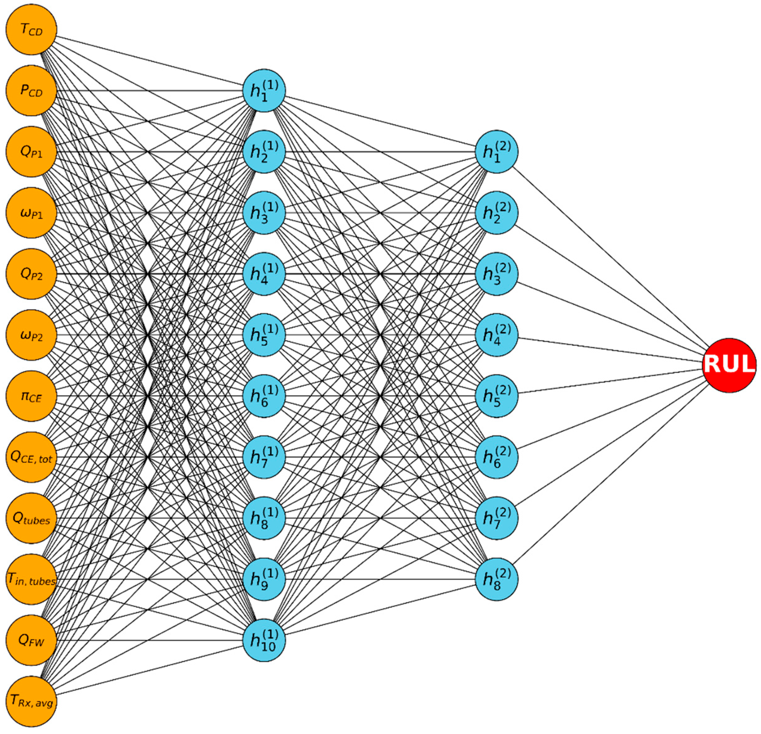
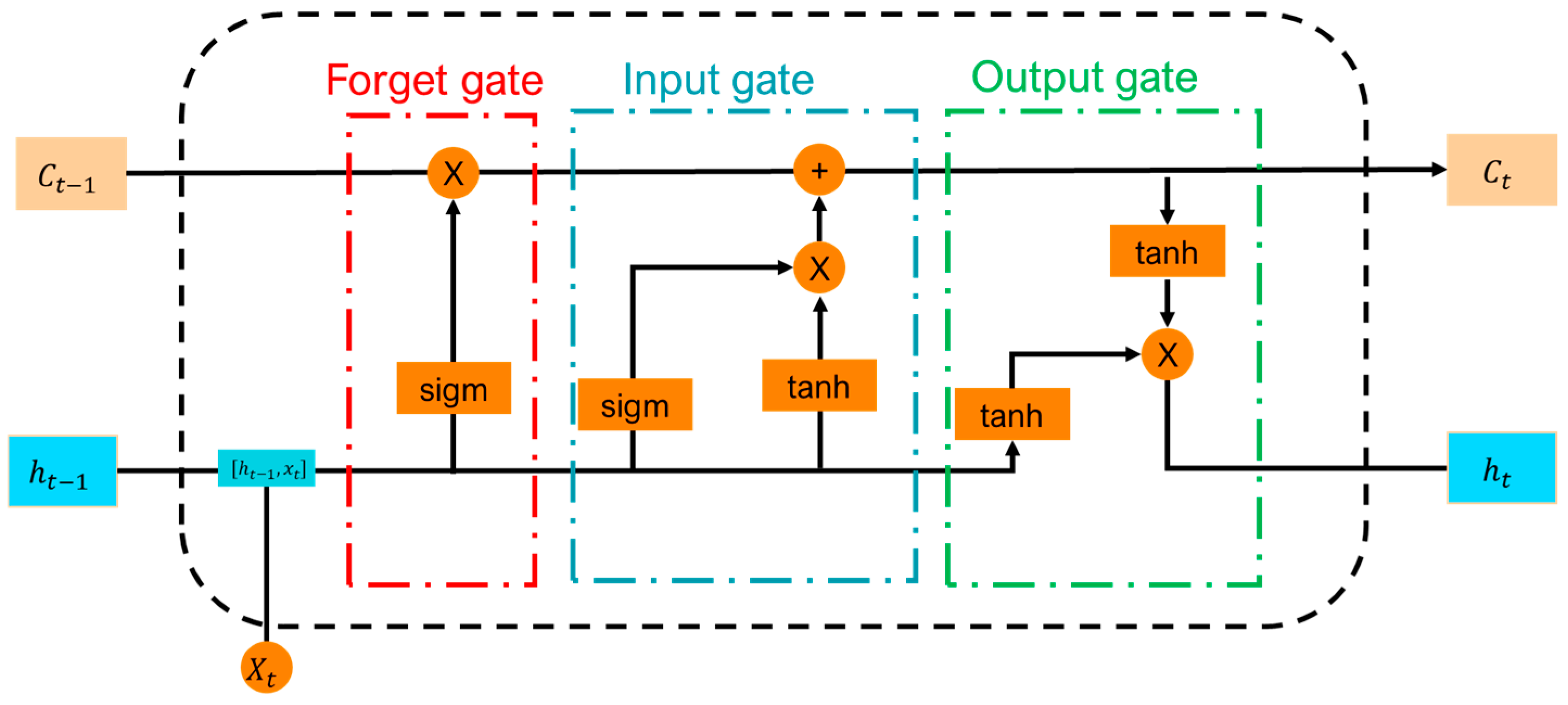
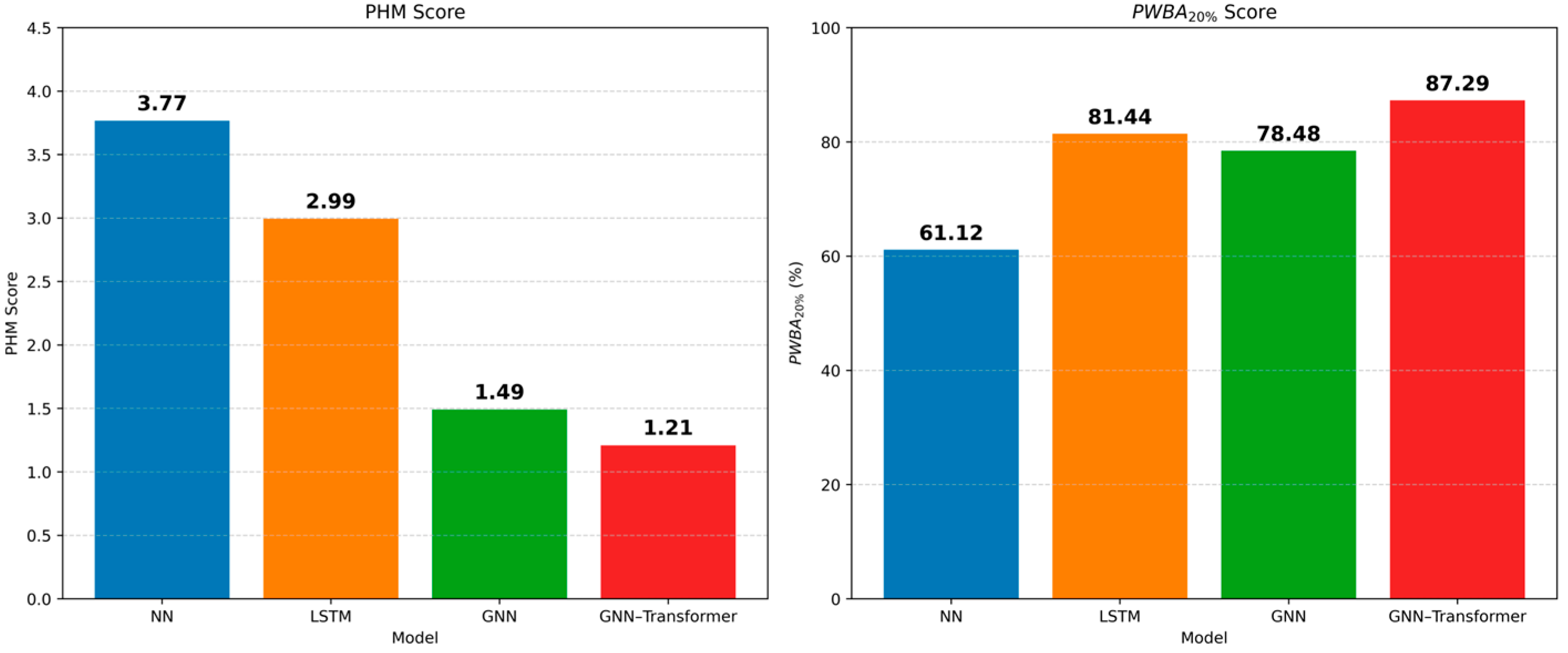
and Figure 6 provide a comprehensive comparison of the predictive performance in the two tests (ensembles 5 and 6) and the computational cost of the four evaluated models. In terms of accuracy, the proposed GNN–Transformer achieves the best overall performance, yielding the lowest MAPE (13.94%) and PHM score (1.21), together with the highest $\mathrm{P}\mathrm{W}\mathrm{B}{\mathrm{A}}_{20\%}$ value (87.29%), indicating both improved precision and robustness in RUL prediction. The LSTM model ranks second, substantially outperforming the baseline NN with a reduced MAPE and higher $PWB{A}_{20\% }$, while the standalone GNN notably improves the PHM score by effectively modeling the system topology, despite a higher MAPE than the LSTM. 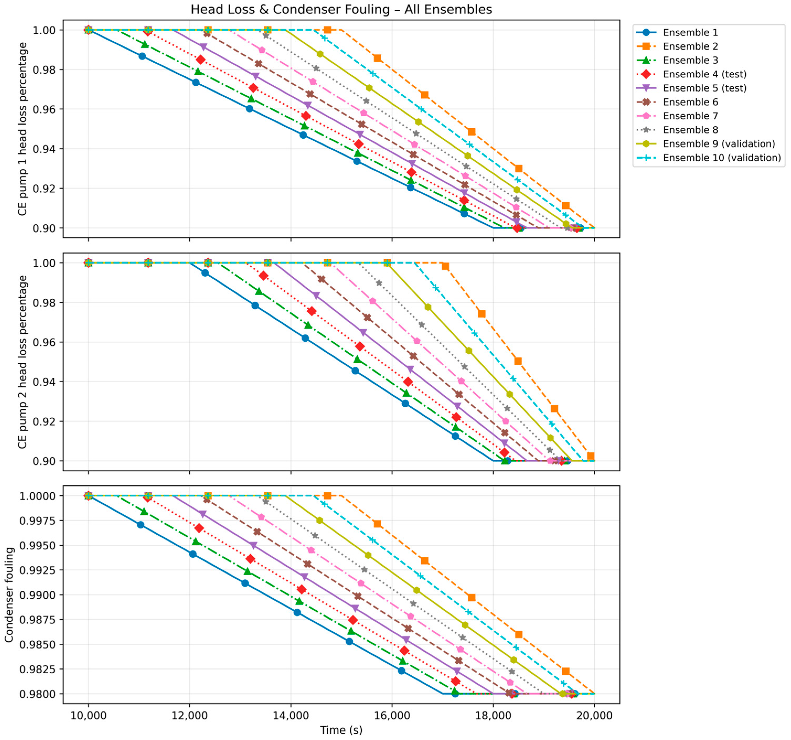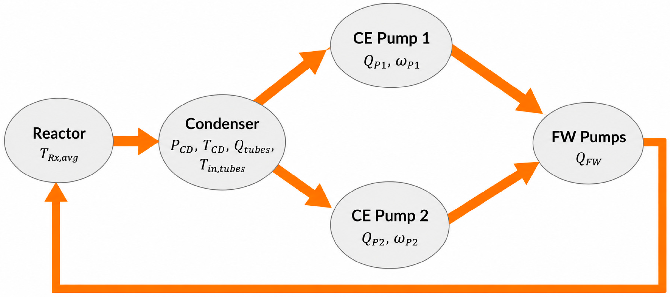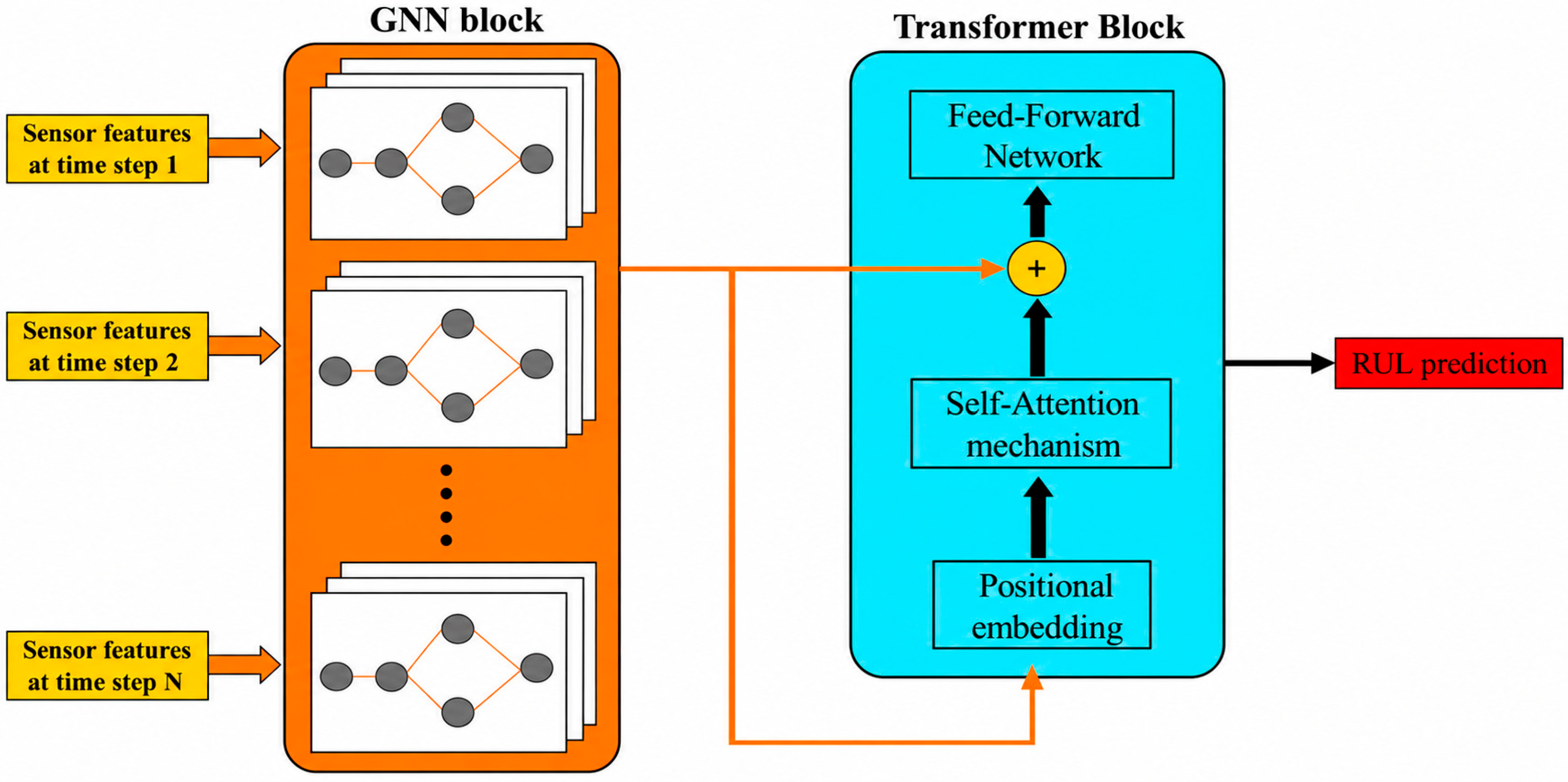As shown in Figure 6, the GNN–Transformer clearly dominates both the PHM score and $PWB{A}_{20\% }$, demonstrating the effectiveness of the proposed spatiotemporal architecture. Unlike conventional neural networks, the proposed GNN–Transformer exploits the physical characteristics of the degradation process. Condenser fouling progressively reduces heat-transfer performance, leading to an increase in condenser pressure that propagates through the coupled balance-of-plant components, including the circulating and condensate extraction pumps. Consequently, the degradation manifests as correlated changes across multiple subsystems rather than isolated variations in individual sensor signals. The graph neural network captures these physical interactions by constraining information exchange according to the plant topology, allowing degradation information to propagate only along physically meaningful connections. The Transformer complements this representation by modeling the gradual temporal evolution of these coupled responses over extended operating periods, enabling the network to recognize long-term degradation trends that precede the end-of-life condition. This combination contributes to the superior predictive performance of the proposed architecture by enabling the model to exploit the physical interactions among plant components and their long-term degradation behavior more effectively than models that consider only temporal information or independent sensor measurements. From a computational perspective, the GNN–Transformer achieves superior performance at a higher computational cost, as reflected in its substantially longer optimization time (4215.9 s) and increased inference latency (4.1 ms). It is important to note that the optimization and training times of sequence-based models, particularly the LSTM and GNN–Transformer, are strongly dependent on the input window size used to capture temporal dependencies, and therefore scale with the length of the historical sequence considered. In contrast, the NN and GNN models exhibit lower optimization overhead and very fast inference times. Despite these differences, the inference latency remains low for all evaluated models, indicating that each approach is suitable for real-time condition monitoring applications. Overall, these results highlight a trade-off between predictive accuracy and computational efficiency, with the GNN–Transformer offering the most accurate and robust predictions while requiring greater computational resources during training and optimization.

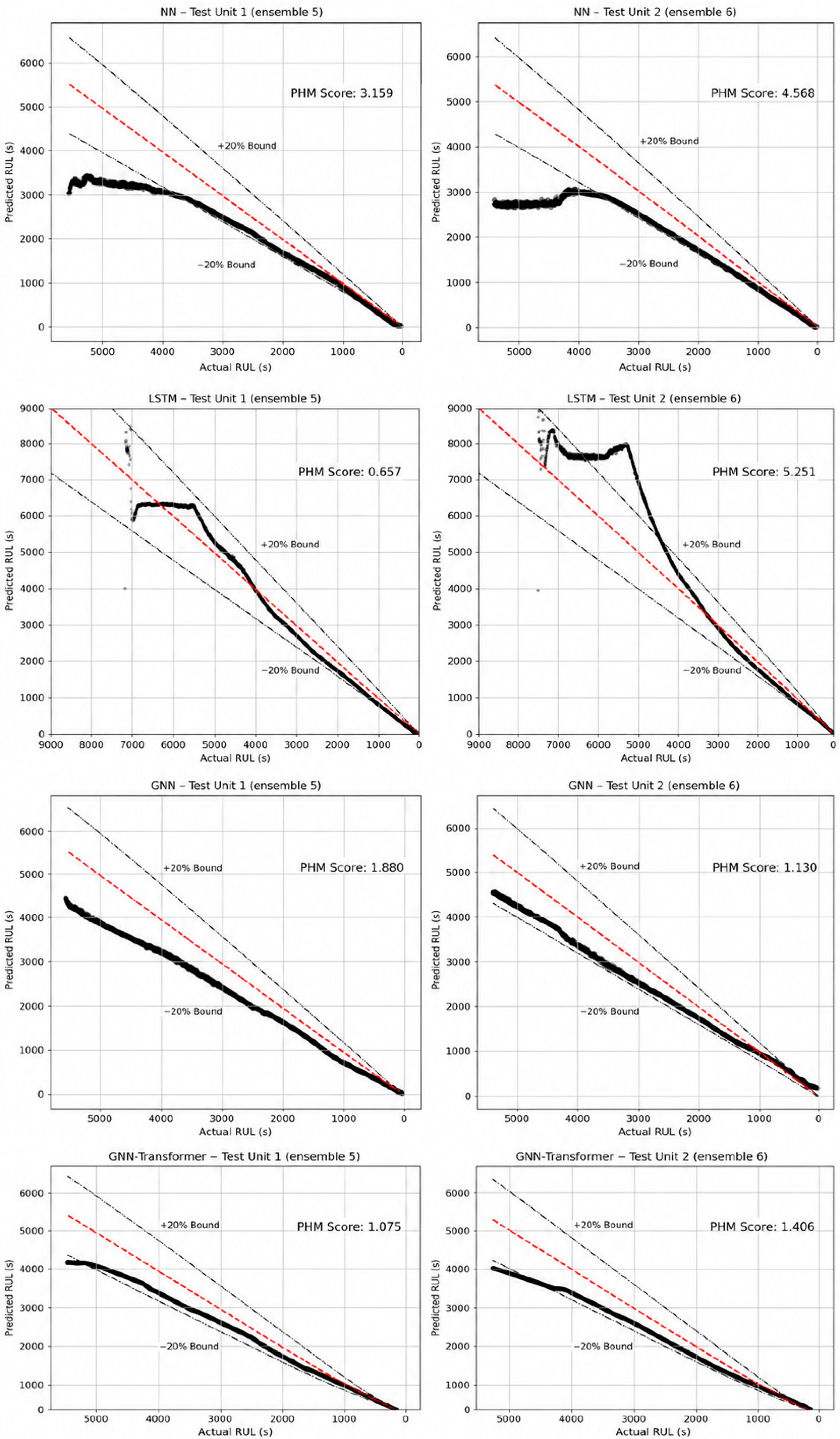
Figure 7 illustrates the predicted RUL versus the actual RUL for the four models evaluated on the two test datasets (Ensembles 5 and 6), together with the ideal prediction line and the ±20% error bounds. The baseline NN exhibits a clear bias, with large dispersion at higher RUL values and a significant number of predictions falling outside the ±20% bounds, consistent with its relatively poor PHM score. The LSTM improves the overall trend alignment and captures part of the temporal degradation behavior; however, its predictions show noticeable oscillations and abrupt changes in the high-RUL region, leading to increased variance and several violations of the error bounds. In contrast, the GNN produces smoother and more consistent predictions across the entire RUL range, with a substantial reduction in scatter and improved adherence to the ±20% bounds, demonstrating the benefit of explicitly modeling system topology. The proposed GNN–Transformer further refines this behavior, yielding predictions that closely follow the ideal diagonal over both test ensembles, with minimal dispersion and the highest concentration of points within the ±20% bounds. Overall, the figure highlights the progressive improvement in RUL estimation achieved by incorporating spatial dependencies through GNNs and long-term temporal modeling through the Transformer, particularly under unseen operating conditions.

To isolate the impact of temporal attention from that of explicit graph topology, a standalone Transformer baseline was also implemented. This model operates directly on standardized multivariate time windows without a preceding GNN stage. At each time step, the input sequence is first processed by a positional embedding layer that projects sensor measurements into a latent representation and adds learnable positional encodings. The resulting sequence is then passed through a single Transformer encoder block with multi-head self-attention and a position-wise feed-forward subnetwork, followed by global average pooling over time and two fully connected layers that map the aggregated representation to a scalar RUL prediction. Hyperparameters such as the number of attention heads, feed-forward dimension, learning rate, batch size, and number of training epochs are optimized with Optuna using the same search ranges summarized in Table 5, ensuring that differences in performance between the standalone Transformer and the GNN–Transformer primarily reflect the presence or absence of explicit graph topology rather than unequal tuning effort. When evaluated on the test ensembles, the standalone Transformer achieved a $PWB{A}_{20\%}$ of 84.71% and a PHM score of 1.86, whereas the topology-aware GNN–Transformer achieved a $PWB{A}_{20\%}$ of 87.29% and a PHM score of 1.21. The improved performance demonstrates the benefit of incorporating topology-aware graph embeddings in addition to temporal attention for further reducing risk-weighted errors and increasing tolerance-based accuracy.

4.3. Metrics Uncertainty Quantification

Uncertainty quantification (UQ) plays a critical role in RUL prognostics, as machine learning–based models are inherently sensitive to the quantity, diversity, and representativeness of the available training data. In practical prognostic applications, RUL predictions are often required under extrapolative conditions and limited historical observations, where overconfident yet inaccurate estimates may lead to unsafe maintenance decisions. Therefore, beyond point-wise accuracy, it is essential to assess the confidence associated with model predictions and to explicitly quantify uncertainty in order to support reliable and risk-aware decision-making.

In the present work, predictive uncertainty is quantified using a deep ensembles approach [24], which is particularly effective for capturing epistemic uncertainty arising from model approximation error and finite training data. The deep ensembles consist of training M independent instances of the same machine learning model, with M = 5 in this study. All ensemble members share the same optimal hyperparameters identified through Optuna-based hyperparameter optimization, ensuring that differences among ensemble predictions are driven solely by data resampling and stochastic training effects rather than suboptimal model configurations. Model diversity is introduced by varying both the random initialization seed and the composition of the training dataset through story-level bootstrap resampling.

Since the data used in this study are generated from a deterministic Simulink-based simulator, the inherent aleatoric uncertainty associated with measurement noise and stochastic system behavior is considered negligible. Consequently, the uncertainty estimated by the deep ensembles primarily reflects epistemic uncertainty, which is directly related to model confidence and is expected to decrease with additional training data or improved model expressiveness.

This uncertainty quantification framework is applied to two representative models: the baseline NN, which exhibited the weakest predictive performance in the deterministic evaluation, and the proposed GNN–Transformer model, which achieved the best overall accuracy. By analyzing both the least and most performant models, the proposed UQ analysis provides insight into how predictive uncertainty evolves with model complexity and representational capacity, and how confidence estimates correlate with predictive performance.

In this application, predictive performance under uncertainty is evaluated using both point accuracy and coverage-based reliability metrics. The MAPE, defined in Equation (5), is computed using the ensemble mean prediction as the point estimate, thereby reflecting the expected RUL prediction across multiple model realizations. While MAPE quantifies average relative accuracy, it does not provide information regarding the reliability of the associated uncertainty estimates. Therefore, the Prediction Interval Coverage Probability (PICP) is additionally employed to assess uncertainty calibration. Let $\overline{y_i}$ denote the ensemble mean prediction at sample iii and let $\sigma$ denote the corresponding ensemble-based predictive standard deviation. A symmetric prediction interval is constructed as

$$[\overline{y_i}-z{\sigma }_i, \overline{y_i}+z{\sigma }_i]$$

(11)

where the scaling factor is set to 2 in this work. This choice corresponds to a $\pm 2\sigma$ interval, which under a Gaussian assumption provides a nominal coverage of approximately 95%, and is commonly adopted in prognostics and health management literature to balance interval sharpness and coverage reliability. The PICP is then defined as the fraction of true RUL values that fall within this interval:

$$PICP\left(\%\right)={\displaystyle \frac{100}{N}} {\displaystyle {\sum }_{i=1}^N}\mathsf{{\rm I}} (y_i\in [\overline{y_i}-z{\sigma }_i, \overline{y_i}+z{\sigma }_i\left]\right)$$

(12)

where $\mathsf{{\rm I}}$ denotes the indicator function, equal to 1 if the condition is satisfied and 0 otherwise, and N is the number of data points.

Together, MAPE and PICP provide complementary insight into the accuracy and empirical coverage of ensemble-based RUL predictions. While PICP quantifies the empirical coverage of the prediction intervals, it does not indicate whether the prediction intervals are unnecessarily wide. Therefore, the Mean Prediction Interval Width (MPIW) [25] is additionally evaluated to quantify interval sharpness. The MPIW is defined as:

$$MPIW=\left(1/N\right) {\displaystyle {\sum }_{i=1}^N}\left(U_i-L_i\right)$$

(13)

where $U_i$ and $L_i$ denote the upper and lower prediction bounds for sample i, respectively, and N is the total number of test samples. Lower MPIW values indicate sharper prediction intervals, although they should be interpreted together with PICP to avoid overly narrow intervals with poor empirical coverage. Furthermore, the Continuous Ranked Probability Score (CRPS) [26] is additionally evaluated. Assuming a Gaussian predictive distribution, the CRPS is computed as

$$CRPS={\displaystyle \frac{1}{N}}{\sum }_{i=1}^N{\mathsf{\sigma }}_i\left[z_i\left(2\mathsf{\Phi }\left(z_i\right)-1\right)+2\mathsf{\varphi }\left(z_i\right)-{\displaystyle \frac{1}{\sqrt{\mathsf{\pi }}}}\right]$$

(14)

where

$$z_i={\displaystyle \frac{y_i-\overline{y_i}}{{\mathsf{\sigma }}_i}}$$

(15)

is the standardized prediction error, $N$ is the total number of test samples, $y_i$ is the true RUL, $\overline{y_i}$ is the ensemble mean prediction, and ${\sigma }_i$ is the corresponding predictive standard deviation estimated from the deep ensembles. Furthermore, $\varphi \left(z_i\right)$ and $\mathsf{\Phi }\left(z_i\right)$ denote the probability density function (PDF) and cumulative distribution function (CDF) of the standard normal distribution, respectively. The standardized error $z_i$ measures the deviation between the predicted mean and the true RUL relative to the predicted uncertainty. Consequently, CRPS evaluates the quality of the entire predictive distribution, simultaneously rewarding accurate predictions, well-calibrated uncertainty estimates, and sharp prediction intervals, while penalizing both overconfident predictions (intervals that are too narrow) and unnecessarily conservative predictions (intervals that are excessively wide). Lower CRPS values, therefore, indicate higher-quality probabilistic predictions.

The quantitative results summarized in

Table 7. Average deep-ensemble MAPE, Mean Prediction Interval Width (MPIW), Prediction Interval Coverage Probability (PICP), and Continuous Ranked Probability Score (CRPS) on the test dataset for the NN and GNN–Transformer models.

Model	Avg. MAPE (%)	Avg. PICP (%)	Avg. MPIW	Avg. CRPS
NN	19.39	40.50	1089.01	446.08
GNN–Transformer	10.92	89.99	1289.24	222.63

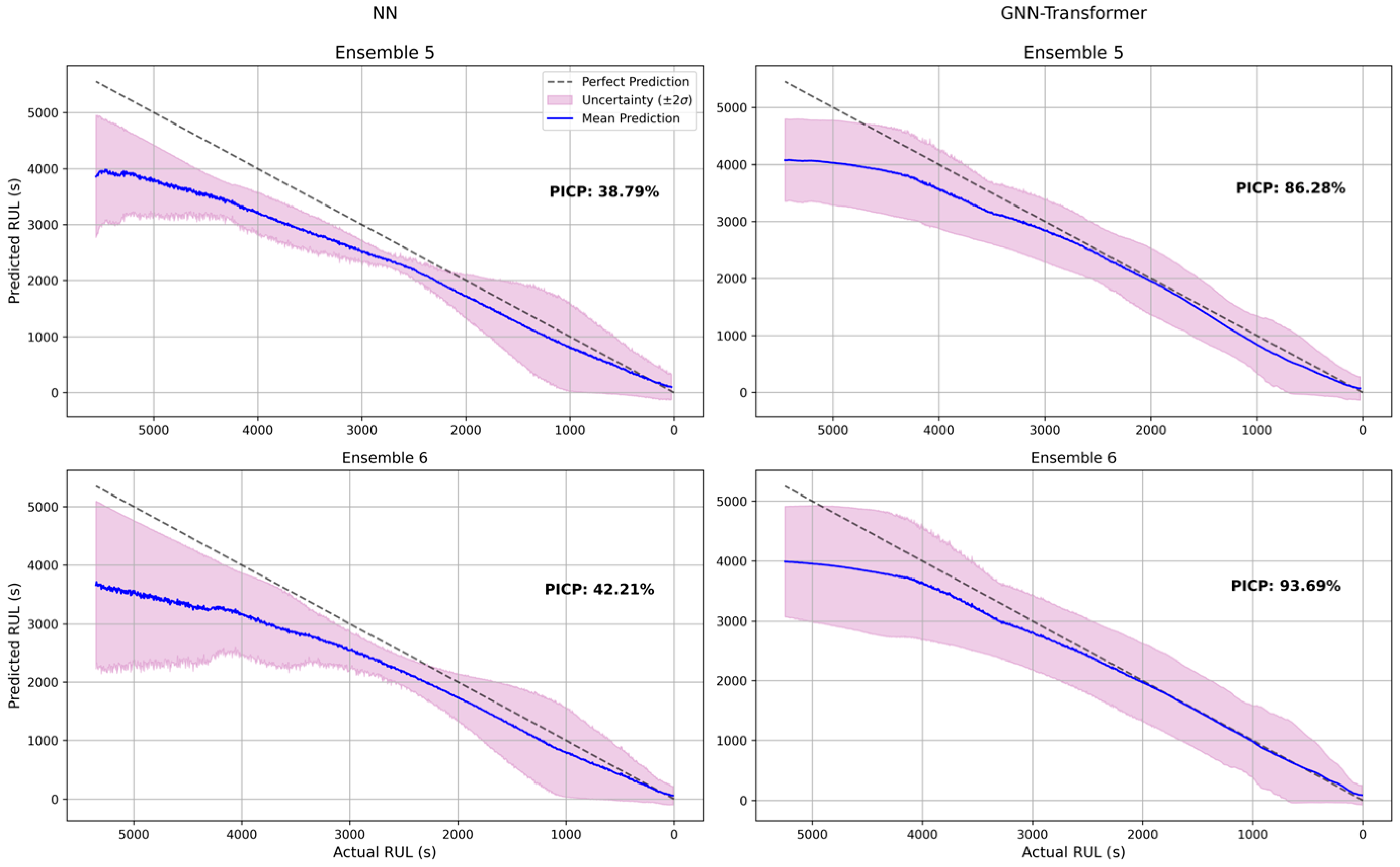
and the uncertainty visualizations shown in Figure 8 highlight a marked contrast between the baseline NN and the proposed GNN–Transformer in terms of both predictive accuracy and uncertainty calibration. The performance values reported in Table 7 correspond to the metrics averaged over the two test ensembles (Ensembles 5 and 6). As reported in Table 7, the NN exhibits a high average MAPE of 19.39%, together with a low average PICP of 40.50% and a relatively large average CRPS of 446.08. This indicates not only poor point-wise accuracy but also severely overconfident uncertainty estimates, with more than half of the true RUL values falling outside the predicted ±2σ intervals. The poor uncertainty calibration of the baseline NN can be attributed to its limited representational capability. Because the model processes each observation independently, without explicitly incorporating either the temporal evolution of the degradation process or the physical interactions among plant components, it exhibits larger systematic prediction errors and reduced diversity among ensemble members. As a result, the predicted uncertainty intervals are frequently too narrow to encompass the true RUL trajectory, leading to the observed low PICP despite the use of the same deep-ensemble uncertainty quantification strategy. This behavior is clearly reflected in Figure 8, where the ensemble mean prediction deviates substantially from the ideal prediction line, and the uncertainty bands frequently fail to capture the true degradation trajectory, particularly in the early and mid-life regions.

In contrast, the GNN–Transformer achieves a substantially lower average MAPE of 10.92% while simultaneously attaining a high average PICP of 89.99%, demonstrating a significantly improved balance between accuracy and uncertainty reliability. This improvement is further supported by the uncertainty metrics reported in Table 7. Although the GNN–Transformer exhibits a moderately larger average MPIW (1289.24) than the baseline NN (1089.01), indicating slightly wider prediction intervals, it simultaneously achieves a substantially higher PICP (89.99% versus 40.50%) while reducing the average CRPS from 446.08 to 222.63, representing approximately a 50% reduction. Whereas MPIW evaluates interval sharpness and PICP measures empirical coverage, CRPS assesses the quality of the entire predictive distribution by jointly evaluating prediction accuracy, calibration behavior, and interval sharpness. Consequently, the combination of higher PICP, moderately increased MPIW, and substantially lower CRPS indicates that the improved uncertainty performance is achieved through more reliable and better-calibrated probabilistic predictions rather than simply increasing the prediction interval width. As shown in Figure 8, the ensemble mean predictions closely follow the ideal diagonal across both test ensembles, and the predicted uncertainty bands consistently enclose the true RUL trajectory throughout most of the degradation process. Notably, the uncertainty intervals of the GNN–Transformer remain well-calibrated without becoming excessively wide, indicating improved confidence estimation rather than conservative over-coverage. Overall, these results demonstrate that increased model expressiveness, achieved through the joint modeling of system topology and long-term temporal dependencies, leads not only to more accurate RUL predictions but also to substantially better-calibrated epistemic uncertainty estimates. The combined analysis of Table 7 and Figure 8 confirms that the proposed GNN–Transformer provides both reliable point predictions and trustworthy uncertainty quantification, which are essential requirements for safe and informed decision-making in prognostic applications.

5. Conclusions and Future Work

This study presents a unified, spatiotemporal machine learning framework designed to predict the RUL of highly interconnected systems within nuclear power plants. Recognizing that degradation mechanisms propagate through complex physical pathways, this work evaluated standard NN, LSTM networks, GNN, and a novel hybrid GNN–Transformer architecture using degraded operational datasets generated by the ASHERAH simulator. The results indicate that accurate RUL prediction benefits from simultaneously modeling the physical relationships among plant components and their temporal degradation behavior. By combining graph-based representations of system topology with transformer-based temporal attention, the proposed GNN–Transformer achieved the best overall performance across the evaluation metrics considered in this study. These findings demonstrate the potential of topology-aware spatiotemporal machine learning for RUL prognostics of interconnected nuclear power plant subsystems, particularly in the balance-of-plant and condenser region considered in this work. However, the present work should be regarded as a simulation-based methodological demonstration; additional validation using higher fidelity models and operational plant data is required before considering application to maintenance decision-making or safety-related analyses. Accordingly, operational benefits often associated with improved RUL prediction—such as safely extending component life, avoiding unplanned shutdowns, or supporting outage optimization—represent potential future benefits contingent on such validation, rather than outcomes demonstrated by the present simulation-based results. Beyond point-estimate accuracy, this study highlights the critical importance of UQ for safe, risk-aware decision-making in predictive maintenance. Through a deep-ensemble methodology, the GNN–Transformer exhibited vastly superior epistemic uncertainty calibration compared to the baseline NN. While the NN produced severely overconfident predictions with an average PICP of just 40.50%, the GNN–Transformer maintained an average PICP of 89.99% and a reduced average MAPE of 10.92%, ensuring reliable confidence bounds across the entire degradation trajectory.

Future research will therefore focus on bridging the gap between simulation and real-world deployment. Subsequent efforts will evaluate the model under more complex fault regimes, including simultaneous multi-component degradation and transient operational anomalies, to test robustness under highly asymmetric fault conditions. Additionally, exploring advanced architectures such as Mixture-of-Experts (MoE) models or specialized gated ensembles could enable dynamic routing of predictions across distinct operating regimes. There is also significant potential to integrate physics-informed constraints directly into the loss function to ensure that predictions strictly adhere to known thermohydraulic conservation laws. Finally, future work will address the computational optimization of sequence-based architectures and transition to empirical validation using historical sensor data from operational nuclear facilities to verify the transferability of the learned topological representations.