Article

A Hybrid Deep Learning Approach for Small-Sample TOC Prediction in Saline Lacustrine Shale

1
State Key Laboratory of Petroleum Resources and Engineering, China University of Petroleum (Beijing), Beijing 102249, China
2
College of Geosciences, China University of Petroleum (Beijing), Beijing 102249, China
3
School of Geosciences, China University of Petroleum (East China), Qingdao 266580, China
4
Exploration and Development Research Institute, SINOPEC, Beijing 100083, China
*
Authors to whom correspondence should be addressed.
Energies 2026, 19(14), 3360; https://doi.org/10.3390/en19143360
Submission received: 23 April 2026 / Revised: 7 July 2026 / Accepted: 8 July 2026 / Published: 16 July 2026

Abstract

Total organic carbon (TOC) is a key parameter for geological sweet spot optimization and resource evaluation. However, accurate TOC prediction remains challenging under small-sample conditions because conventional physical and machine learning methods are commonly limited by insufficient labeled data. To address this problem, this study proposes a hybrid deep learning framework that integrates a convolutional autoencoder with a BP neural network (CAE-BPNN). In this framework, the CAE is first used to learn representative feature expressions from abundant unlabeled logging data, and the learned encoder is then transferred to the supervised prediction stage, where labeled samples are used for TOC prediction through the BPNN. The dataset includes 177 measured TOC samples and 1388 unlabeled logging samples from the Fengcheng Formation shale in Well MY1, in the Mahu Sag, and data from Well MY2 are used for independent validation. Model performance is evaluated using five-fold cross-validation with the coefficient of determination (R2) and root mean square error (RMSE) as metrics. For Well MY1, CAE-BPNN achieves the best performance, with R2 = 0.89 and RMSE = 0.061, outperforming CNN (R2 = 0.85, RMSE = 0.075), GBDT (R2 = 0.83, RMSE = 0.076), RF (R2 = 0.81, RMSE = 0.082), and BPNN (R2 = 0.77, RMSE = 0.085). In the independent validation using Well MY2, CAE-BPNN also shows superior predictive performance, with R2 = 0.81 and RMSE = 0.367. These results indicate that unlabeled logging data can effectively enhance feature representation and improve TOC prediction accuracy under limited labeled-sample conditions. The proposed method provides an effective solution for small-sample TOC prediction and offers a reliable basis for movable oil evaluation using the oil saturation index (OSI), as well as a reference for predicting other geological parameters such as S1, S2, and porosity.

1. Introduction

The exploration and development of shale oil have become the hottest research topic in the global oil and gas field industry. It is estimated that the recoverable reserves of shale oil in the world are much higher than those of conventional oil. However, compared with marine shale oil in the United States, lacustrine shale oil is mainly developed in China, which is characterized by frequent thin interbeds, strong heterogeneity, and complex organic matter enrichment patterns [1,2,3,4,5]. These characteristics pose significant challenges for geological sweet spot evaluation and resource potential assessment in shale oil. TOC is a key organic geochemical indicator for micro-migration evaluation and for identifying effective source rocks [6,7]. Accurate determination of TOC is critical for geological sweet spot evaluation in shale oil. However, TOC is typically measured in the laboratory. Consequently, acquiring continuous along-profile TOC variation requires extensive regional coring over large longitudinal extents. This process demands substantial time and financial investment. Moreover, constrained by various practical limitations, the quantity of core samples obtained is often insufficient to meet the requirements of tasks demanding substantial TOC data [8,9,10,11]. Since the change in TOC can be reflected by a variety of logging curves (GR, SP, AC, etc.) [12], the acquisition of logging data is easier. Therefore, it is an effective method to predict TOC by establishing the relationship model between logging curves and TOC [13,14,15].
TOC prediction approaches include physical models and data-driven methods. Passey et al. [16] proposed the widely used ΔlogR method. The method first defines two baselines where resistivity and porosity logs coincide and then computes TOC. Subsequently, many researchers have continuously improved ΔlogR to enhance the prediction accuracy. Passey et al. [17] improved the ΔlogR method, significantly enhancing its predictive performance in over-mature reservoirs. Zhao et al. [18] replaced the theoretical baseline with an approximate linear baseline based on the change of the slope of acoustic wave and resistivity with time, thereby improving the prediction effect of ΔlogR. Based on the dynamic baseline theory, Zhu et al. [19] calculated two ΔlogR values by using the acoustic curve with TOC information and the theoretical acoustic curve, and proposed a double-difference ΔlogR method. Zhou et al. [20] proposed the ΔLogR-GR method by combining the ΔlogR method and the natural gamma method. Although the above traditional methods and improved methods are simple and easy to use and have certain interpretability, this series of methods also have some shortcomings: (1) subjectivity in selecting the required parameters; (2) excessive dependence on a single logging curve, so that it cannot fully tap the hidden information of the logging curve; (3) when dealing with complex nonlinear relationships, there are problems of insufficient capacity and heavy workload.
With the advent of the era of artificial intelligence (AI), AI has also made many achievements in the field of oil and gas, such as sedimentary reservoirs, logging evaluation, geophysical exploration, reservoir engineering, and CO2 storage [21,22,23,24,25,26]. Nowadays, the methods of predicting TOC are basically data-driven [27,28]. The commonly used methods include Gaussian regression, RF, support vector machine, GBDT, BPNN, and CNN [21,29,30,31]. Many scholars have applied various combinations of optimization algorithms and traditional models to regression prediction, so a variety of hybrid models have emerged, including the combination of the Bayesian regularization algorithm and BPNN [32]; the particle swarm optimization algorithm combined with support vector machines [33]; the combination of the genetic algorithm and BPNN [34]; the deep belief network combined with long short-term memory networks [35]; and the combination of principal component analysis technology and neural networks [36]. In the past, when doing TOC prediction tasks, whether it is a single model, a traditional model based on different optimization algorithms for parameter adjustment, or a traditional model using feature processing algorithms, most of them belong to the category of supervised learning. In the prediction of TOC, although the results of these models are very good, their performance is highly dependent on the quantity and quality of labeled data. However, geological experimental data are often not easy to expand, and data quality problems are difficult to fully control, which may lead to insufficient learning and training of the model. In addition, when these models are applied to new areas with large differences in geological conditions, the stability and generalization ability of the models are often insufficient, so that the accuracy will be greatly reduced. The above situations are generally the common problems of previous TOC prediction models. Therefore, it is urgent to solve the problem of insufficient model generalization ability and prediction accuracy of small-sample TOC prediction tasks.
The quality of the model prediction results is directly related to the feature engineering [37,38]. Especially for the small-sample regression prediction task, the processing of features is more important [39]. The logging curve used to predict TOC is easy to obtain, the amount of data is large, and it is related to many physical parameters. The natural and unsupervised learning characteristics are appropriate. The advantage of unsupervised learning is that it can independently learn the potential information of unlabeled data (logging data without measured TOC). It focuses on deep mining at the feature level, which can extract more sufficient and effective feature expression from the original data. Therefore, considering the use of logging curves without measured TOC as the input of unsupervised learning, it is expected to break through the dependence on measured labels and extract more valuable deep information for TOC prediction. To this end, this study proposes a convolutional autoencoder-BP neural network (CAE-BPNN) method, which is an end-to-end learning framework that combines unsupervised learning and supervised learning, making full use of the advantages of unsupervised learning. This method is mainly aimed at small-sample learning tasks to obtain more accurate prediction results and significant generalization ability, and it is rarely applied to TOC prediction. Because the geological logging data has the characteristics of time series correlation and local distribution, convolution can extract the important characteristics of logging data [40]. Therefore, in the unsupervised stage of this study, an autoencoder based on convolution operation is adopted. First, the model learns the effective representation of the input data, and then automatically extracts the most discriminative features through the reconstruction process [41]. Subsequently, these learned features are input into the back-end TOC predictor. The predictor adopts a dual-path structure: the main part performs the main prediction task based on the BPNN, while the branch part introduces the residual network to enhance the representation ability of the model and optimize the training process. This end-to-end hybrid model has reference significance for solving the problem of physical parameter prediction under small-sample conditions, and also provides innovative technical support for the quantitative evaluation of TOC in lacustrine shale oil.
Compared with existing TOC prediction methods, the proposed CAE-BPNN framework is designed to address geological heterogeneity and limited labeled samples in saline lacustrine shale oil reservoirs. Conventional ΔlogR-based methods are physically interpretable but sensitive to baseline selection and local petrophysical assumptions [16,17,18,19,20], whereas data-driven methods such as RF, GBDT, BPNN, CNN, SVM, and GPR generally depend on sufficient labeled TOC samples and may become unstable when laboratory measurements are sparse [21,27,28,29,30,31]. Recent small-sample and semi-supervised studies have demonstrated the potential of unlabeled logs for representation learning [40,42,43]. Building on this concept, this study integrates unsupervised CAE pretraining, supervised BPNN fine-tuning, and a residual branch to learn transferable logging representations from 1388 unlabeled samples while using only 177 measured TOC samples for calibration. This framework is applied to the Fengcheng Formation shale in the Mahu Sag, where strong reservoir heterogeneity and limited training samples challenge conventional models. Its prediction accuracy and generalization ability are evaluated across two wells and compared with RF, GBDT, CNN, and BPNN using R2 and RMSE. The results show that CAE-BPNN can reduce the effects of heterogeneity and label scarcity, providing a practical approach for small-sample prediction of TOC and related geological parameters.

2. Convolutional Autoencoder-BP Neural Network Model

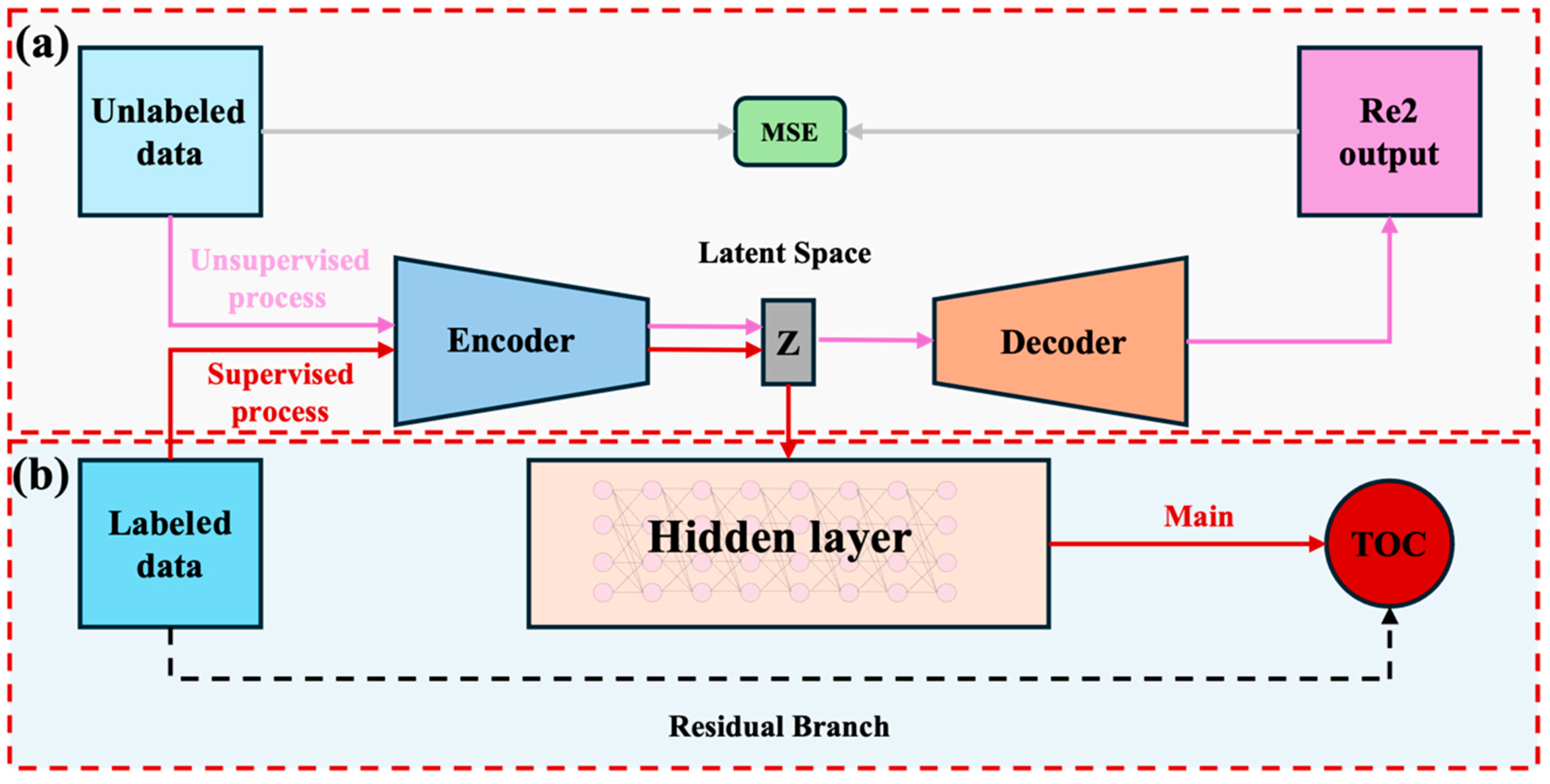
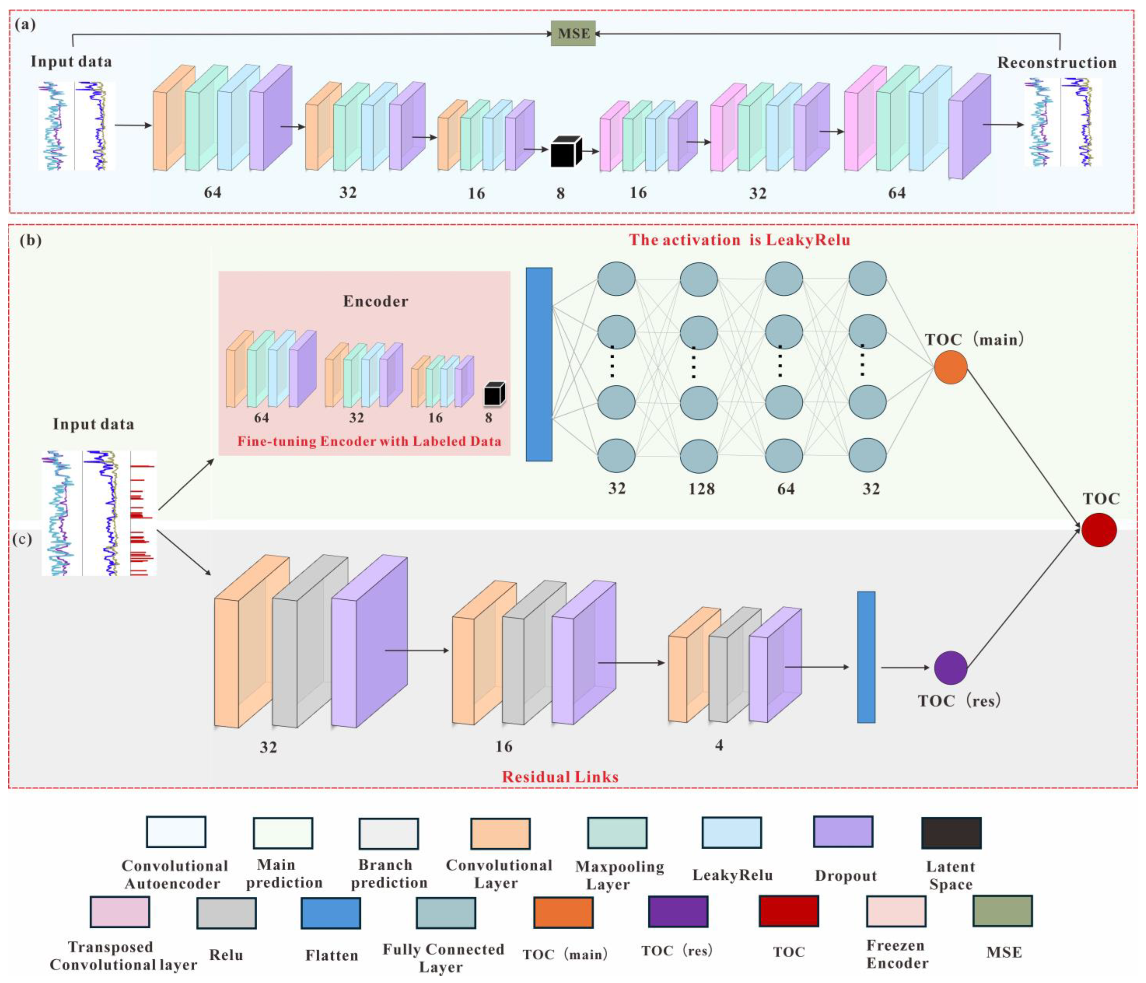
In this study, a two-stage learning framework is employed to integrate unsupervised feature extraction with supervised TOC prediction. The end-to-end regression model, which jointly leverages labeled and unlabeled logging data and integrates a CAE with a BPNN, incorporates features learned during the unsupervised stage, thereby mitigating label scarcity in small-sample settings and enhancing the model’s generalization. The workflow is illustrated in Figure 1.
(1)
Data preparation stage: The dataset comprises labeled samples with TOC annotations and unlabeled logging data.
(2)
CAE training stage: The model is first initialized, after which the CAE is trained on unlabeled data to learn intrinsic feature relationships, reconstruct the input features, and minimize the reconstruction loss between the input and its reconstruction (Figure 1a).
(3)
TOC prediction stage: In the backbone, the pretrained CAE is fine-tuned on the labeled data, and the encoder outputs are fed into a BPNN to yield the backbone prediction; in the residual branch, a skip connection is applied to estimate the residual and generate the residual prediction. The final prediction is obtained by summing the backbone and residual outputs (Figure 1b).

2.1. Convolutional Autoencoder

Building on the traditional autoencoder, the CAE (Figure 1a) is an unsupervised learning framework well suited for feature dimensionality reduction, extraction, and denoising. Its architecture consists of two mirror-symmetric components: an encoder and a decoder. The encoder uses convolutional operations to compress the input into a compact latent-space representation. Subsequently, the decoder employs transposed convolutions to reconstruct the original input from this latent representation, which may require cropping to align spatial dimensions [41,44]. Training minimizes the discrepancy between the original input and its reconstruction, typically measured by the mean squared error (MSE) loss.
(1)
Encoder: The encoder maps the input to a low-dimensional latent space that captures principal feature relationships and preserves the salient information of the original data.
z = f encoder Conv X
where X denotes the input data; Conv denotes the convolution; z denotes the potential space.
(2)
Decoder: The decoder maps the low-dimensional latent representation back to the original feature space to reconstruct the input data.
X ^ = f decoder DeConv z
where   X ^   denotes the output of the reconstruction; DeConv denotes the transposed convolution.
(3)
Training objective: Minimize the MSE between the input and the reconstructed output, thereby enabling the model to learn intrinsic relationships among features.
L M S E = | X X ^ | 2
where L M S E denotes the MSE loss function.

2.2. BP Neural Network Model

BPNN constitutes a multi-layer feedforward architecture that employs error backpropagation for parameter optimization. This network utilizes a dual mechanism: forward propagation transmits input signals to generate outputs, while backward propagation distributes error signals to update network weights [45]. BPNN is adept at handling complex nonlinear relationships encountered in engineering research and demonstrates robust performance in diverse applications including data classification, clustering, and regression analysis.
A typical BPNN structure comprises an input layer, one or more hidden layers, and an output layer (Figure 1b). Neurons within each layer are densely interconnected with all neurons in the subsequent layer, forming a fully connected topology. The output from a preceding layer serves as the input to the following layer. The core training principle relies on the error backpropagation algorithm, which iteratively adjusts connection weights and neuron thresholds to minimize the discrepancy between predicted and target outputs. During training, if the network output deviates significantly from the expected value, the input data is reprocessed. The algorithm systematically refines the connection strengths and thresholds between the input and hidden layers and between the hidden and output layers until the prediction error falls within an acceptable tolerance, signifying convergence. Networks trained via this method exhibit strong nonlinear mapping capabilities and possess a flexible structure adaptable to various problem domains.

3. An Application Example for Shale Oil

3.1. Field Background

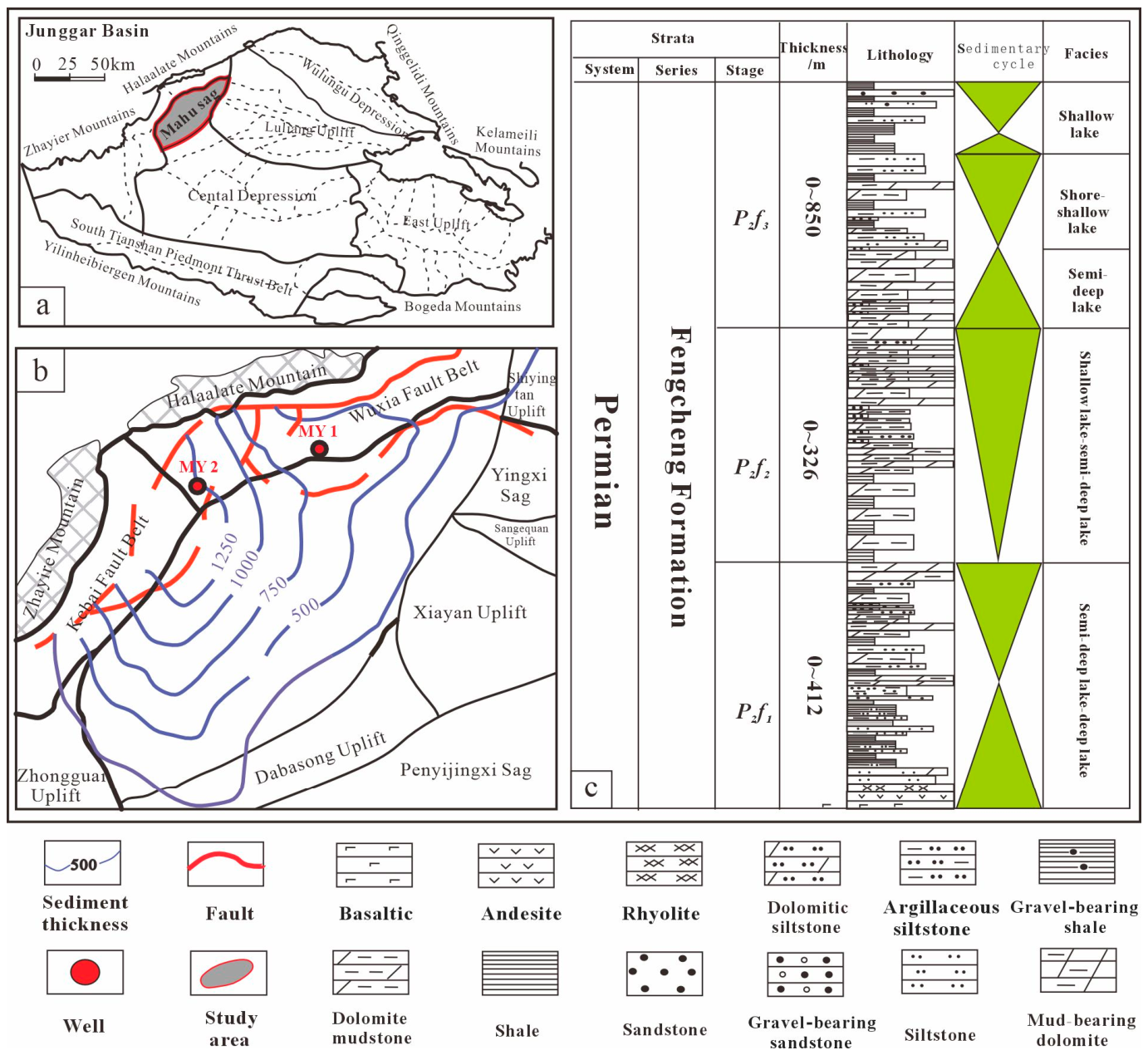
The Junggar Basin (Figure 2a), located in northwestern China, is a key junction of three paleoplates and has experienced multiple tectonic cycles. Multiple superposed source-rock sets across its structural units collectively control the basin’s extensive, complex hydrocarbon distribution [46]. As one of the basin’s most active sags, the Mahu Sag (Figure 2b) occupies the northwestern part of the Central Sag and covers approximately 5000 km2 [47]. It is bounded by the Baikouquan Fault Zone to the west and the Xiazijie Fault Zone to the east; adjacent uplifts include the Dabasong and Zhongguai uplifts, with the Xiayan and Sansanquan uplifts farther east and the Shuitan Uplift to the northeast [42].
This study focuses on the Lower Permian Fengcheng Formation (P1f) source rocks in the Mahu Sag (Figure 2c). Deposited in a fan-delta–lacustrine system, the formation is widespread, thick, and wedge-shaped, thickening northwestward. Stratigraphically, it comprises three members (ascending): P1f1, P1f2, and P1f3. P1f1 mainly consists of massive basalt, dolomitic mud shale, and argillaceous siltstone; local sodium carbonate indicates incipient alkaline-lake deposition. P1f2 is dominated by argillaceous dolomite, dolomitic shale, argillaceous siltstone, and alkali-bearing shale; abundant alkaline minerals mark the peak of alkaline-lake evolution. The lower P1f3 comprises interbedded argillaceous dolomite and dolomitic shale, grading upward into coarse fan-delta clastic; reduced dolomite and alkaline minerals indicate the waning of alkaline-lake conditions [43,48]. Overall, the Fengcheng Formation records an alkaline lacustrine setting with frequent laminated mud-shale interbeds, pronounced rhythmicity, and maturation from low to high during hydrocarbon generation and expulsion, establishing prerequisites for a prolific petroleum system.

3.2. Related Work

Well logging is the most widely used technique in petroleum exploration. Its high vertical resolution allows lithology to be identified from logging curves; variations in logging responses correlate with organic matter content [12,14,15]. To predict TOC accurately, the effects of different logging curves must be analyzed, and key curves selected as input features.
During feature selection, core depths must be corrected. Depth-measurement errors arise from different compression coefficients of the cable and drill pipe, causing mismatches between core and logging depths [30]. Feature selection follows two criteria: prior experience and R2. R2 quantifies the correlation between logging curves and TOC. Together, these criteria determine the final input features. R2 can be calculated using the following equation:
R 2 = 1 i = 1 n y i y i ^ 2 i = 1 n y i y ¯ 2
where   y i   denotes the true value; y i ^   denotes the predicted value; y   ¯ denotes the mean value for all samples.
It should be emphasized that the R2 analysis was used as an initial screening tool rather than as the sole criterion for feature selection. A low single-variable linear R2 does not necessarily indicate the absence of information in a multivariate nonlinear model, because weakly correlated logs may still contain complementary geological signals or interact nonlinearly with other curves. Therefore, GR, AC, CNL, and DEN were retained by jointly considering linear correlation, logging availability, data quality, petrophysical meaning, and previous TOC-logging studies [12,15,27,28]. The four curves reflect organic-matter enrichment, lithology/mineral composition, porosity, compaction, and hydrogen-bearing components from different perspectives. Nevertheless, the limited number of input channels constrains the representation capacity of the CAE, and future work should add mutual information, SHAP-based feature attribution, variance inflation factor analysis, and sensitivity tests to further quantify nonlinear information content and multicollinearity [27,28,49].
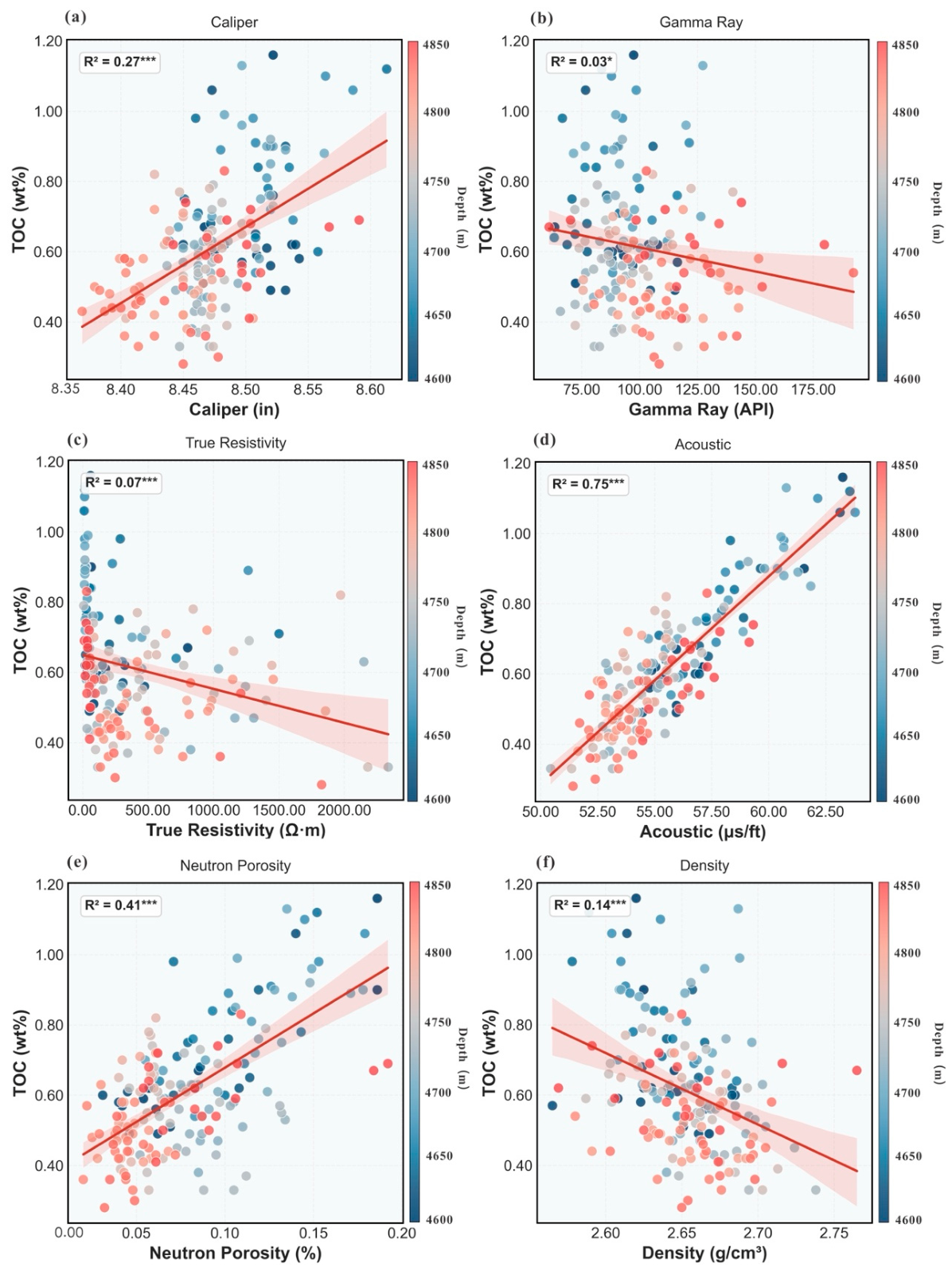
The correlation between TOC and logging curves is measured by R2 (Figure 3). Sonic travel time, neutron porosity, and borehole caliper show positive correlations with TOC, whereas gamma ray, resistivity, and density show negative correlations. These patterns accord with local lithology, organic matter occurrence, and reservoir evolution. The R2 for AC and TOC is 0.75 (Figure 3d). Organic rich shale contains abundant organic pores and microcracks, so compressional waves attenuate and travel time increases. The R2 for CNL and TOC is about 0.41 (Figure 3e), reflecting a higher hydrogen index. Organic matter, especially kerogen and adsorbed hydrocarbons, is hydrogen-rich and oxygen-poor, which yields apparently high neutron porosity. The R2 between CAIL and TOC is about 0.27 (Figure 3a), consistent with washouts in organic rich layers caused by low drill ability. The R2 values for DEN, GR, and RT with TOC are about 0.14, 0.03, and 0.07, respectively (Figure 3b,c,f), indicating low sensitivity due to mineral composition, fluid properties, and thermal evolution in the Fengcheng Formation. Although GR and DEN show relatively weak single-variable linear correlations with TOC in the Fengcheng Formation, they were retained because GR, AC, CNL, and DEN are widely recognized as effective conventional logs for TOC prediction and can jointly reflect shale content, lithology/mineral composition, acoustic response, hydrogen-bearing components, porosity, compaction, and organic-matter enrichment; thus, weak linear correlation does not necessarily exclude their complementary value in a multivariate nonlinear model [12,15,27,31]. Based on these results and previous work, the selected input features included GR, AC, CNL, and DEN.
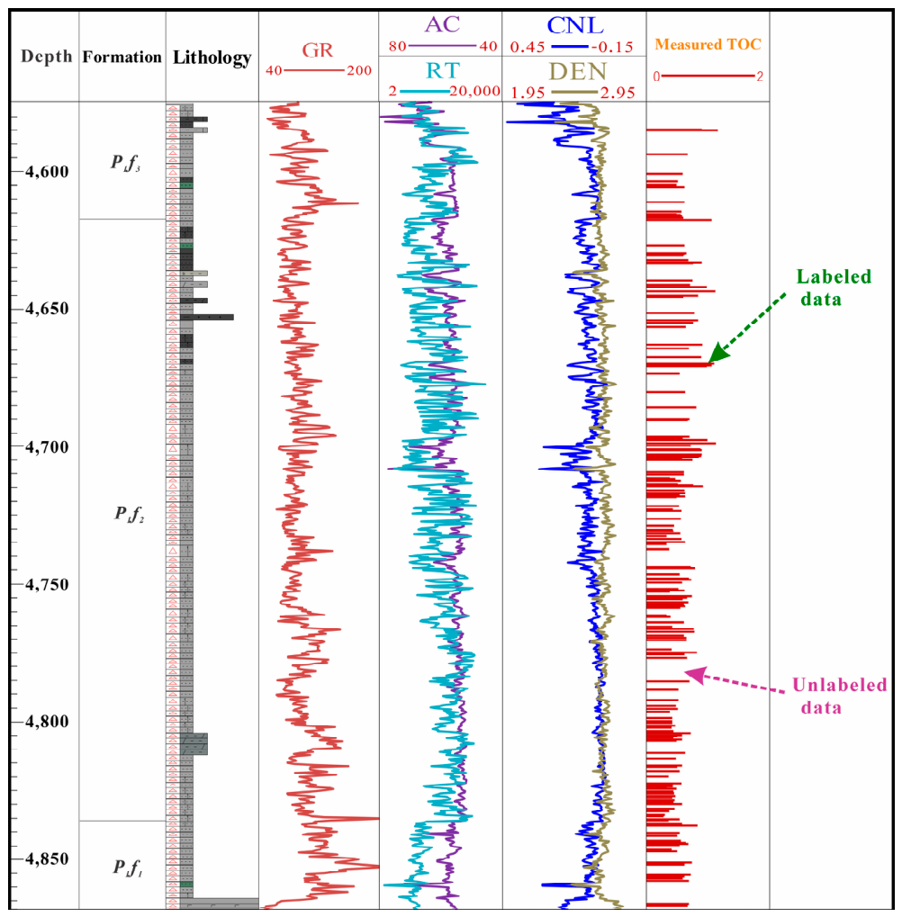
After identifying the required input features, the dataset was organized. The data were split into labeled and unlabeled sets based on the presence of measured TOC (Figure 4). Both sets included the selected logging curves. The labeled set contained 177 Fengcheng Formation samples with measured TOC and corresponding logs. The unlabeled set contained logs for 1388 Fengcheng Formation samples and no measured TOC. Before model training, missing values and outliers were checked. Input features were standardized to unify scale, yielding zero mean and unit standard deviation. To avoid potential information leakage during cross-validation, all data-driven preprocessing and model-fitting procedures were controlled within each training fold. Specifically, the mean and standard deviation used for feature standardization were estimated only from the training subset and then applied to the corresponding validation subset. CAE pretraining and supervised fine-tuning were performed using training-fold data only, and the validation fold was used only for model evaluation. The main model settings were fixed before final cross-validation and kept consistent across folds to reduce fold-specific overfitting. Standardization can be calculated using the following equation:
X = x μ σ
where x denotes the input data; μ represents the mean; σ denotes the standard deviation; X denotes standardized data.
In this study, the small-sample problem is quantitatively defined by the limited number of labeled samples available for supervised learning: only 177 samples have measured TOC labels, whereas 1388 logging samples do not have TOC measurements. The labeled samples account for approximately 11.3% of all MY1 logging samples used in the learning workflow. This imbalance is typical in geological prediction because laboratory geochemical measurements are much more expensive and less continuous than well logs [8,9,10,11]. The unlabeled samples were therefore used only for unsupervised representation learning by the CAE, whereas supervised TOC calibration was performed using the labeled samples.
To avoid information leakage during cross-validation, all data-driven preprocessing steps should be performed within each training fold. Specifically, the mean and standard deviation used for feature standardization should be fitted only on the training subset and then applied to the corresponding validation subset. CAE pretraining, hyperparameter selection, and BPNN fine-tuning should also be conducted using training-fold data only; the validation fold should be used only for model evaluation.
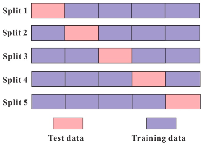
In the evaluation stage of TOC prediction, five-fold cross-validation is used (Figure 5), and root mean square error and R2 serve as evaluation metrics. Cross-validation reduces dependence on a single partition and uses limited data more fully, producing more stable and reliable estimates. RMSE measures the difference between predictions and observations and is sensitive to outliers, which aids assessment in extreme cases. A smaller RMSE indicates better predictive performance. R2 reflects the goodness of fit. Values closer to one indicate a better fit to the data. Using both metrics provides a more comprehensive and reliable evaluation of predictive ability. R2 was shown in Equation (4). The RMSE can be calculated using the following equation:
RMSE = 1 n i = 1 n y i y i ^ 2
where y i denotes the true value; y i ^   denotes the predicted value.

3.3. Building Convolutional Autoencoder-BP Neural Network Model

A CAE BPNN model is proposed. In the unsupervised stage, unlabeled logging data are used, and a CAE performs feature learning. The encoder input layer takes four logging curves: AC, CNL, GR, and DEN. As shown in Figure 6a, the convolutional part has four layers. The kernel size is 3. The numbers of neurons are 64, 32, 16, and 8. The decoder mirrors the encoder and contains four transposed convolution layers. The numbers of neurons are 8, 16, 32, and 64. The output layer reconstructs the input. Each layer is followed by BatchNorm, ReLU, MaxPool, and Dropout (0.2). The final layer uses Tanh to constrain the reconstruction range.
The architecture was designed to balance feature-representation capability and overfitting risk under limited labeled-sample conditions. The four-layer 1D convolutional structure enables hierarchical extraction of local logging-response patterns, while the kernel size of 3 captures short-range vertical variations without introducing excessive parameters. Dropout and weight decay are used as regularization strategies to improve model robustness. In addition, the residual branch preserves part of the original logging information and improves gradient propagation during training. Alternative sequential architectures, such as LSTM and Transformers, were not adopted in this study because the number of labeled TOC samples is limited and the input feature dimension is relatively small. These models generally require larger datasets to robustly learn temporal dependencies and may increase the risk of overfitting under small-sample conditions.
In the supervised stage, the encoder is initialized from the trained autoencoder and fine-tuned on labeled data, while the decoder is discarded; the encoder output then serves as the input to the BPNN. The BPNN (Figure 6b) comprises four fully connected layers. The numbers of neurons are 32, 128, 64, and 32. Each layer uses BatchNorm, ReLU, MaxPool, and Dropout (0.2). The output layer predicts TOC (main). In parallel, the original features pass through a residual branch (Figure 6c) composed of three convolutional layers [50,51]. The numbers of neurons are 32, 16, and 4, and the activation is Relu. The residual branch predicts TOC (res), and the final TOC prediction is obtained by summing the main and residual outputs.
During training and validation, five-fold cross-validation (Figure 5), the AdamW optimizer, gradient clipping, and an early stopping mechanism with patience set to 30 improve reliability and stability and help prevent overfitting. A cosine annealing learning rate scheduler decreases the learning rate periodically during training, simulates cooling, and helps escape local optima.
(1)
The input features are standardized as described in Equation (5).
(2)
The encoder applies four layers of 1D convolution:
z = f encoder Conv 4 Conv 1 x
h m = MaxPool Dropout R e L U BatchNorm Conv h m 1
h 0 = x
where x denotes the standardized features of the input; BatchNorm denotes the batch normalization; Dropout denotes the regularization; MaxPool denotes the maximum pooling; ReLU denotes the activation function; Conv denotes the convolution.
(3)
The decoder mirrors the encoder. Four layers of transposed convolution are applied, and the final layer uses Tanh to output the reconstructed feature:
d L = f decoder DeConv 4 DeConv 1 z
x ^ = Tan h Linear d L
where DeConv denotes the transposed convolution; Linear denotes the linear processing.
(4)
The autoencoder is trained to minimize a weighted loss between the input and the reconstructed output. MSE is calculated as described in Equation (3).
After training the autoencoder, the encoder is initialized from it and fine-tuned on labeled data, while the decoder is discarded. The BPNN receives the encoded features from the encoder as inputs and processes them through four fully connected layers. The output layer predicts TOC.
(5)
The TOC predictor comprises a prediction backbone and a residual branch. The final prediction is obtained by summing the outputs of the two components.
y main = f fc Flatten z
f n = Dropout R e L U Linear f n 1
f 0 = z
y res = W r x + b r
y ^ = y main + y res
where y main denotes the main branch prediction; y res denotes the prediction of residual branch; Flatten denotes flattening; b r denotes the bias parameter; W r denotes the weight; y ^ denotes the final predicted value.
(6)
Finally, R2 and RMSE are used to evaluate the model; R2 was shown in Equation (4) and RMSE was shown in Equation (6).
The CAE BPNN model is implemented in PyTorch and Scikit Learn.
All experiments were conducted on a standard workstation equipped with an Intel CPU, 32 GB RAM, and an NVIDIA GPU. The model was implemented using Python 3.12, PyTorch 2.4.0, and Scikit-learn 1.5.0. Because the dataset contains only 177 labeled TOC samples and 1388 unlabeled logging samples, the computational cost was moderate. A complete five-fold training and validation process required only several minutes, with peak GPU memory usage below approximately 2 GB, indicating that the proposed framework can be implemented without high-performance computing resources.

3.4. Building BP Neural Network Model

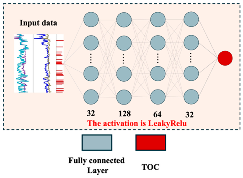
A BPNN without autoencoder derived features was implemented to evaluate the effectiveness of the CAE BPNN. The architecture matches the BPNN described in Section 3.3. As shown in Figure 7, features learned by the autoencoder are not used at input. Standardized features are provided directly to the model.

3.5. Building Convolutional Neural Network Model

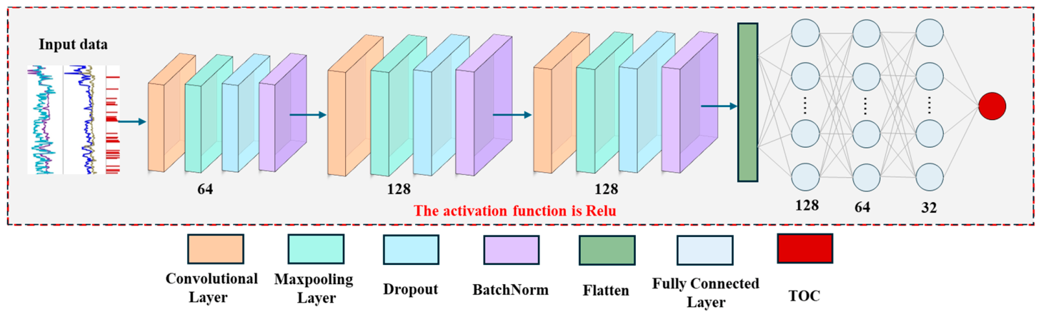
A CNN is used for TOC prediction. CNN can perform well across domains due to local connectivity and feature amplification [31,52]. A deep regression model is designed with multi-layer one-dimensional convolution and fully connected layers. Input features are the optimized set selected in Section 3.2. As shown in Figure 8, the front end uses a three-layer 1D convolutional network. The numbers of kernels are 64, 128, and 128, and the kernel size is 3. Each layer is followed by BatchNorm, ReLU, MaxPool. After flattening, the output feeds a three layer fully connected network. The numbers of neurons are 128, 64, and 32, and the activation is Relu. The final layer is a linear output for TOC regression.
(1)
The input features are standardized as described in Equation (5).
(2)
Three layers of 1D convolution are applied:
H m = Relu BatchNorm Conv X
P m = Dropout MaxPool H m
where X denotes the standardized features; BatchNorm denotes the batch normalization; Dropout denotes the regularization; Relu denotes the activation function; MaxPool denotes the maximum pooling.
(3)
The output from the final convolution and pooling is flattened, followed by a three-layer fully connected network for prediction:
F 0 = Relu Linear Flatten P L
F n = Dropout Relu Linear F n 1
y ^ = Linear f L
where Flatten denotes flattening; Linear denotes the linear processing; y ^ denotes the predicted value of TOC.
(4)
Finally, R2 and RMSE are used to evaluate the model; R2 was shown in Equation (4) and RMSE was shown in Equation (6).
The CNN model is implemented in PyTorch and Scikit Learn.

3.6. Building Machine Learning Model

In addition, other machine learning models were used for TOC prediction, including RF and GBDT.

3.6.1. Building Random Forest Model

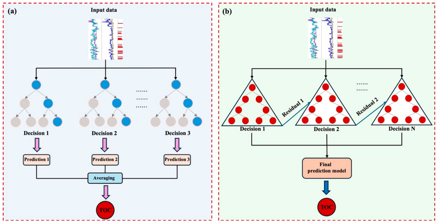
RF is an ensemble machine learning model (Figure 9a). Its decision trees run in parallel, which yields fast computation [53,54]. It has proven effective across many domains. It tolerates outliers and noisy data [55]. Therefore, a multi-parameter RF regression model with tunable hyperparameters is designed for TOC prediction in nonlinear geological logging data. Model inputs are the selected logging curves from Section 3.2. The final core parameters are obtained via cross-validation and GridSearch and are listed in Table 1. The model uses the Bagging ensemble to average predictions from multiple decision trees.
(1)
The input features are standardized as described in Equation (5).
(2)
The RF regressor consists of multiple decision trees. Each tree is trained on a subset drawn from the dataset by Bootstrap sampling. At each node split, a random subset of features is evaluated to find the best split, and the tree then produces a prediction. The final prediction is the average of all tree predictions:
y ^ = 1 M m = 1 M f m x
θ = arg   min θ Θ   MSE CV θ
where   f m x   denotes the prediction of a single tree; M denotes the total number of trees; y ^ denotes the predicted value of TOC; Θ denotes the parameter space; CV denotes cross-validation; θ denotes the hyperparameter combination; arg min denotes the operation of the parameter when the minimum value is taken.
(3)
Finally, R2 and RMSE are used to evaluate the model; R2 was shown in Equation (4) and RMSE was shown in Equation (6).
The RF model is implemented in Scikit Learn.

3.6.2. Building Gradient Boosting Decision Tree Model

GBDT (Figure 9b) is an ensemble learning model that builds multiple decision trees through serial iterations. At each iteration, the newly added tree learns the residuals between current predictions and observed values. By gradually correcting these residuals, overall predictive performance improves [56]. Each subsequent tree focuses on errors left by the existing ensemble. This serial training mechanism enables continuous improvement in prediction performance. Accordingly, GBDT is used for TOC prediction. Model inputs are the logging curves selected in Section 3.2. Core parameters are listed in Table 1. The model adopts a residual fitting strategy, training one tree per iteration to accumulate and refine predictions.
(1)
The input features are standardized as described in Equation (5).
(2)
The model is initialized.
F 0 x = y ¯
where F 0 x denotes the initial predicted value; y ¯ denotes the mean value of the training set target.
(3)
Iterative training includes residual computation, new tree fitting, model updating, and final prediction.
r i m = y i F m 1 x i
h m x r i m
F m x = F m 1 x + γ h m x
y ^ = F M x = F 0 x + m = 1 M γ h m x
where r i m denotes the residual; y i denotes the true value of TOC; F m 1 x i denotes the predicted value of the TOC; h m x denotes the output of the tree; γ denotes the learning rate; y ^ denotes the final predicted value.
(4)
Finally, R2 and RMSE are used to evaluate the model; R2 was shown in Equation (4) and RMSE was shown in Equation (6).
The GBDT model is implemented in Scikit Learn.

4. Results

4.1. Geochemical Characteristics

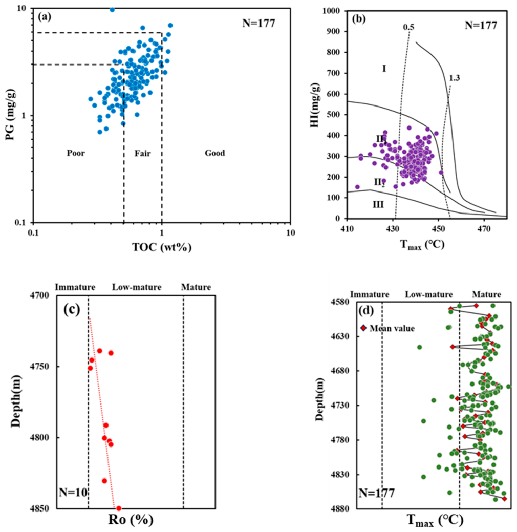
Organic matter abundance is a key indicator of source rock quality (Figure 10a). TOC and hydrocarbon generation potential (PG) are commonly used metrics for assessing organic matter abundance [6]. Among 177 samples, TOC ranges from 0.28% to 1.16%, with a mean of 0.61%. TOC varies widely and is unevenly distributed. PG ranges from 0.70 to 9.71 mg/g, with a mean of 2.46 mg/g. TOC is positively correlated with PG. By TOC criteria for continental source rocks in saline lake basins, most P1f shale cores are good source rocks.
Kerogen is an insoluble product of organic matter degradation and a principal precursor of oil and gas [57]. Shale kerogen types in P1f are classified based on pyrolysis and TOC (Figure 10b). For 177 shale samples, Tmax ranges from 414.5 to 451.11 °C, with a mean of 437.86 °C. HI ranges from 152.32 to 436.89 mg/g, with a mean of 281.50 mg/g. Type II1 kerogen predominates and shows strong oil generation potential.
Vitrinite reflectance Ro (Figure 10c) and Tmax are reliable indicators of thermal maturity [6]. Ro and Tmax are used to evaluate the thermal maturity of P1f shale (Figure 10c,d). Tmax ranges from 414.5 to 451.11 °C, with a mean of 437.86 °C. Ro ranges from 0.71% to 0.89%, with a mean of 0.80%. Overall, Fengcheng Formation shale is in the mature stage.

4.2. Different Models’ Performance

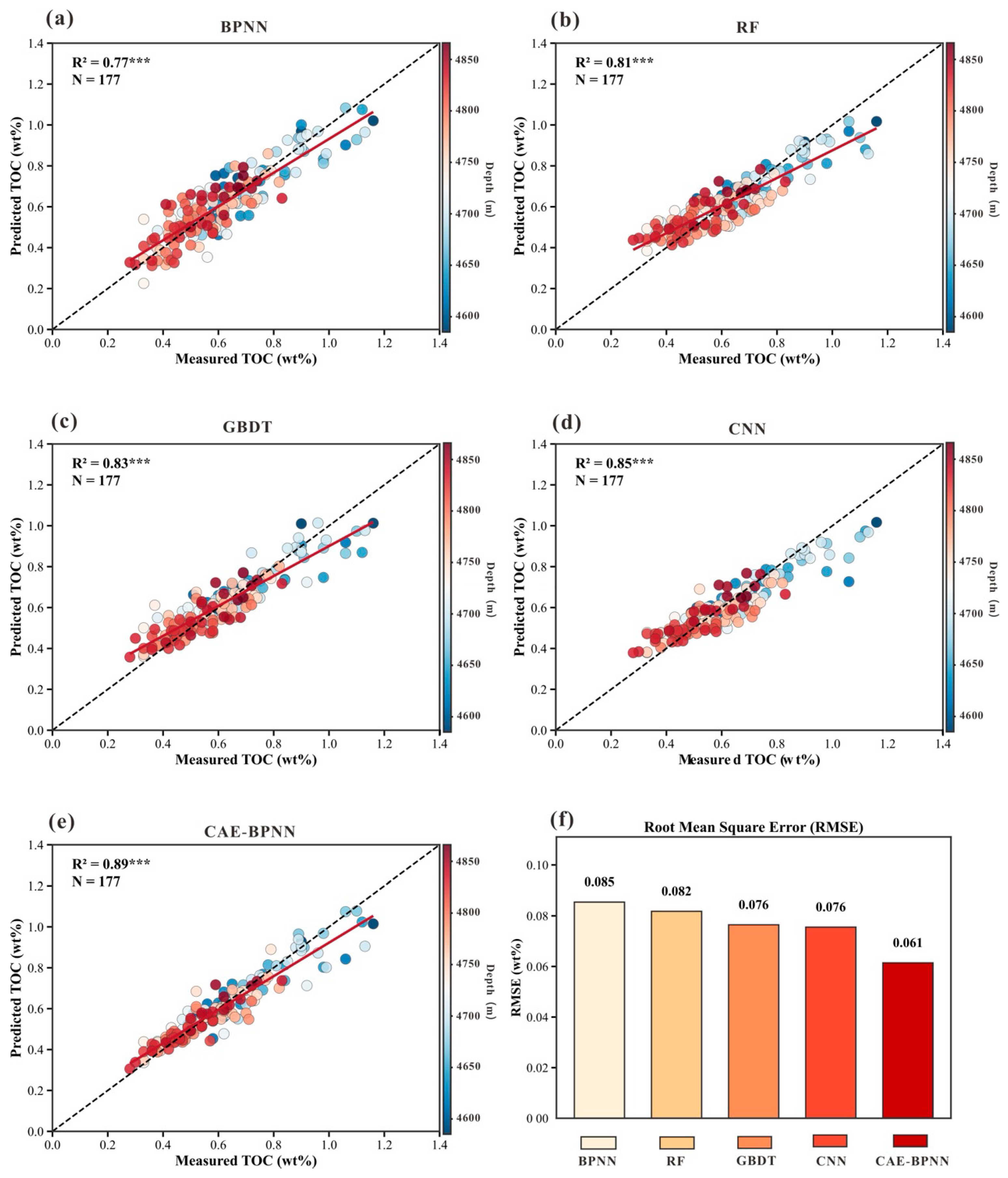
Models for TOC prediction included GBDT, RF, CNN, CAE-BPNN, and BPNN. Predicted TOC values were evaluated. Performance results for each model are shown in Figure 11.

4.2.1. BP Neural Network Model Performance

In Section 3.4, a BPNN was constructed and shows the weakest TOC prediction performance. R2 is 0.77 (Figure 11a) and RMSE is 0.085 (Figure 11f). BPNN is prone to local optima and overfitting with high-dimensional, complex data.

4.2.2. Random Forest Model Performance

In Section 3.6, an RF model was built. R2 is 0.81 (Figure 11b) and RMSE is 0.082 (Figure 11f). RF performs slightly better than BPNN. With high-dimensional, small, or uneven data and outliers, RF can overfit or bias, limiting performance. Overall accuracy and generalization remain below other models.

4.2.3. Gradient Boosting Decision Tree Model Performance

Based on the GBDT in Section 3.6, final evaluation was conducted. R2 is 0.83 (Figure 11c) and RMSE is 0.076 (Figure 11f), outperforming BPNN and RF, and slightly below CNN.

4.2.4. Convolutional Neural Network Model Performance

In Section 3.5, a CNN was built and performs well in TOC prediction. R2 is 0.85 (Figure 11d) and RMSE is about 0.075 (Figure 11f), better than BPNN, RF, and GBDT. Compared with traditional machine learning and fully connected networks, CNN better captures complex structure, nonlinearity, and anomalies. However, performance remains constrained by small-sample regression.

4.2.5. Convolutional Autoencoder-BP Neural Network Model Performance

The CAE-BPNN in Section 3.3 delivers the best TOC prediction, highlighting the benefit of combining abundant unlabeled with limited labeled data. R2 is 0.89 (Figure 11e) and RMSE is 0.061 (Figure 11f), outperforming GBDT, RF, CNN, and BPNN. A convolutional autoencoder reduces dimensionality and extracts deep features from high-dimensional logging data, effectively suppressing redundancy and noise. Compared with BPNN (Figure 11a,f), the unsupervised stage markedly improves modeling efficiency and prediction accuracy. Relative to the best single model, CNN, CAE-BPNN further strengthens feature representation and final prediction performance.
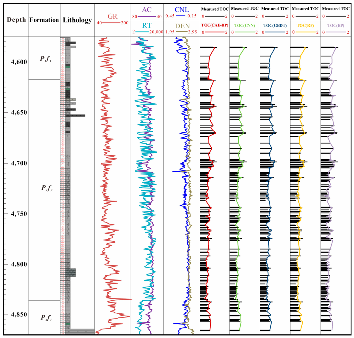
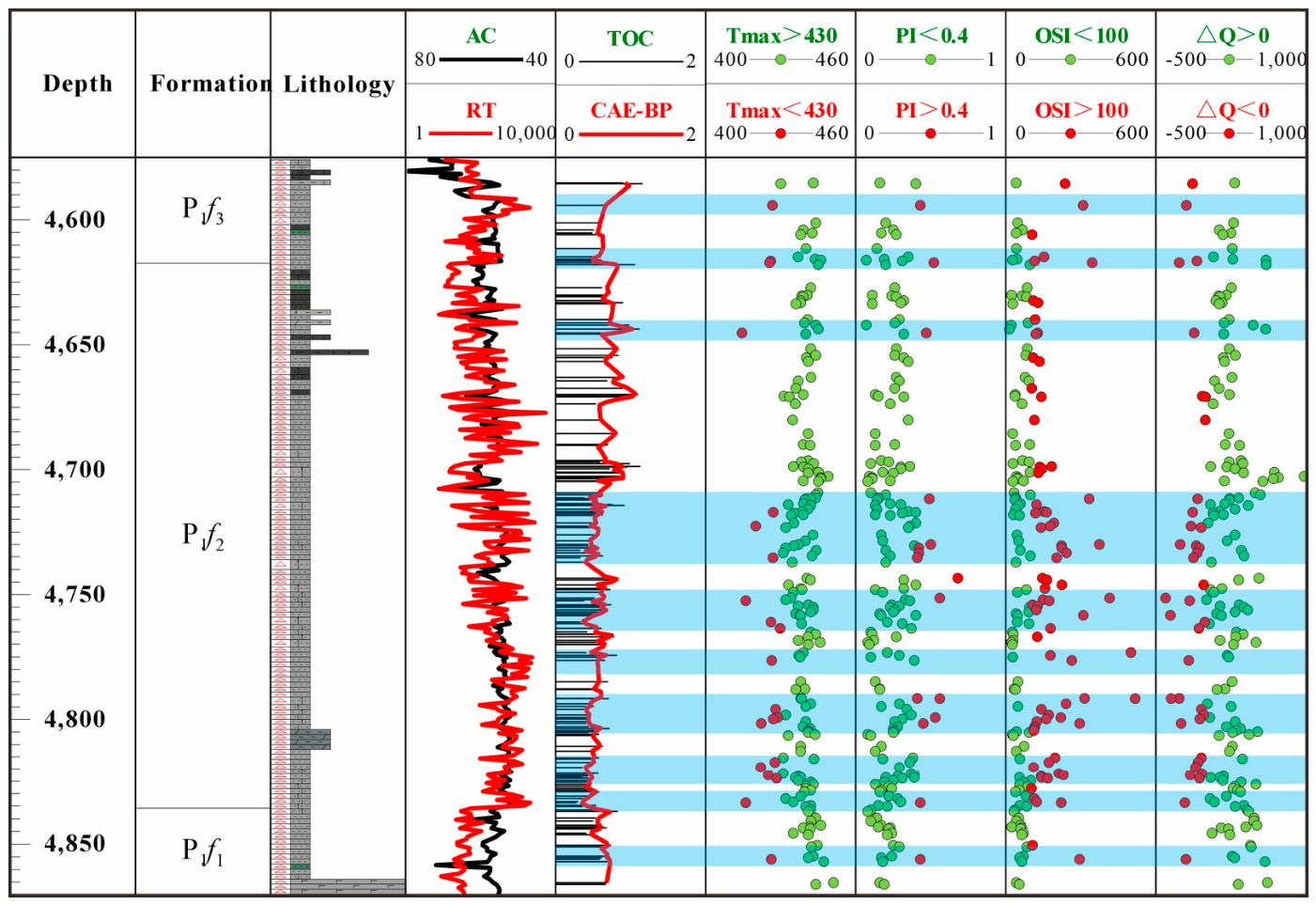
As shown in Figure 12, across the P1f1 to P1f3 interval in the composite log, CAE BPNN aligns most closely with measured TOC, with advantages concentrated in the main P1f2 section and at the P1f1 to P1f2 and P1f2 to P1f3 contacts. It preserves peak and trough fidelity in thin interbeds and noisy zones, avoids over-smoothing and lag, and exhibits smaller bias in low TOC intervals while capturing high TOC spikes better than CNN, RF, GBDT, and BPNN.

4.3. Validation of the Generalization Ability of the Model

Previous model evaluations were conducted mainly using Well MY1, which limited the assessment of model stability and generalization. To provide an independent validation, Well MY2 was selected as an external test well. Geologically, both Well MY1 and Well MY2 are located in the Fengcheng Formation shale of the Mahu Sag and share a similar saline lacustrine depositional background, providing comparable stratigraphic and lithological conditions for TOC prediction. However, as an independent well, Well MY2 exhibits differences in TOC distribution and vertical logging responses relative to Well MY1, reflecting lateral heterogeneity within the Fengcheng Formation. Therefore, Well MY2 is suitable for evaluating the transferability and preliminary generalization ability of the proposed CAE-BPNN model.
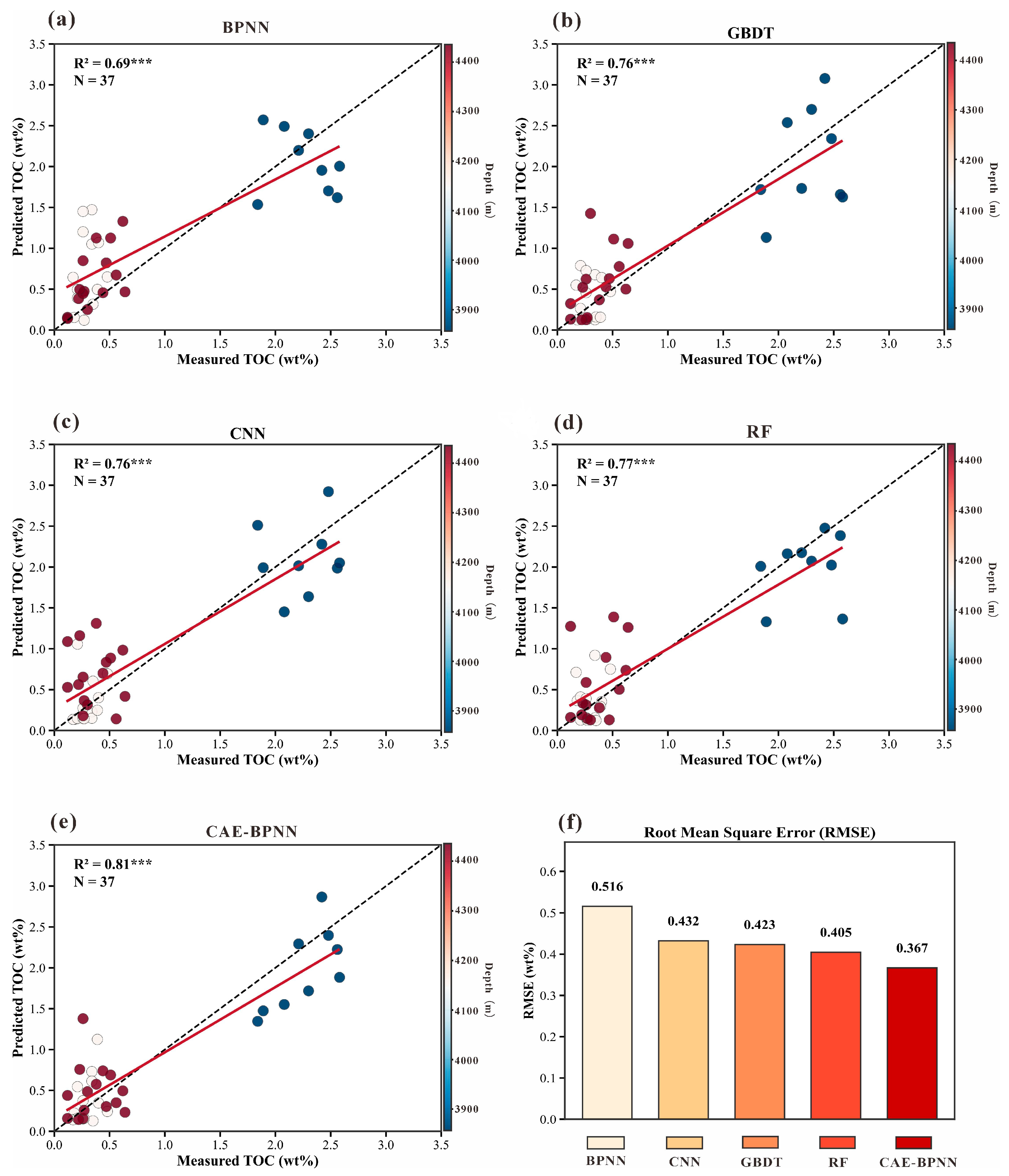
The same five models, including CAE-BPNN, CNN, GBDT, RF, and BPNN, were applied to Well MY2, and the evaluation metrics described in Section 3 were used for comparison. The CAE-BPNN model achieved the best performance, with an R2 of 0.81 and an RMSE of 0.367 (Figure 13e,f). In comparison, CNN obtained an R2 of 0.76 and an RMSE of 0.432 (Figure 13c,f), GBDT achieved an R2 of 0.76 and an RMSE of 0.423 (Figure 13b,f), RF yielded an R2 of 0.77 and an RMSE of 0.405 (Figure 13d,f), and BPNN produced an R2 of 0.69 and an RMSE of 0.516 (Figure 13a,f). These results indicate that CAE-BPNN maintains relatively stable predictive performance in an independent well and outperforms the other models under similar geological conditions. Nevertheless, because the external validation is based on only one additional well, the generalization ability of the model should be regarded as preliminary and requires further verification using more wells and different geological intervals.

4.4. Movability Evaluation of Shale Oil

The oil saturation index (OSI) is a primary indicator of shale oil mobility. Previous studies indicate that an OSI greater than 100 mg/g marks a threshold for mobile oil and favorable development potential [47,58]. A high-precision TOC prediction model based on CAE-BPNN provides a robust basis for mobility evaluation. As shown in Figure 14, the OSI ranges from 14.29 to 517.18 mg/g, with a mean of 110.57 mg/g; more than half of the samples exceed 100 mg/g, indicating generally good mobility. Depth-wise analysis using predicted TOC shows that low TOC intervals coincide with high OSI values above 100 mg/g, implying better shale oil mobility under low organic matter abundance. This pattern is consistent with the low TOC and high mobility relationship documented for P1f in the Mahu Sag. To verify this relationship, the hydrocarbon expulsion potential approach was used to quantify micro-transported hydrocarbons, denoted ΔQ [47]. As shown in Figure 14, ΔQ ranges from negative 403.2 to 981.86 mg/g, with a mean of 188.49 mg/g. Positive ΔQ indicates hydrocarbon expulsion, whereas negative ΔQ indicates external hydrocarbon charging. Spatial correlation with predicted TOC shows that expulsion intervals generally correspond to high TOC and low OSI; conversely, charging intervals are mostly associated with low TOC and high OSI. From a migration dynamics perspective, low TOC intervals act as dominant hydrocarbon acceptors, indicating good shale oil mobility.

4.5. Additional Robustness Checks and Methodological Limitations

Although the fold-averaged R2 and RMSE values indicate that CAE-BPNN achieves the best overall performance among the tested models, the comparison should be interpreted cautiously under small-sample conditions. In this study, model performance was mainly evaluated using five-fold cross-validation and independent-well validation. Because fold-wise residual distributions were not further analyzed, the reported metric differences are interpreted as empirical performance improvements rather than formal evidence of statistical significance. Future studies based on larger multi-well datasets should incorporate repeated cross-validation or bootstrap resampling to estimate confidence intervals and conduct paired statistical tests between CAE-BPNN and baseline models [59].
The contribution of unlabeled data is another important methodological issue. The comparison between BPNN without CAE and CAE-BPNN demonstrates that representation learning from unlabeled logging data can improve TOC prediction. However, the effective minimum amount of unlabeled data is not expected to be a universal fixed percentage. Instead, it depends on geological representativeness, stratigraphic coverage, logging quality, and the distribution of logging responses within the target interval. For CAE pretraining, the unlabeled samples should sufficiently cover the major variations in lithology, mineral composition, porosity, compaction, and organic-matter-related logging responses. In this study, all available high-quality unlabeled samples from the target interval were used to maximize geological coverage and reduce sampling bias. Future work will further evaluate sample-efficiency curves using different proportions of unlabeled data in larger and more diverse datasets.
Model interpretability also remains a limitation of the present framework. Feature importance analysis, SHAP analysis, sensitivity analysis, and latent-space visualization can provide additional evidence for determining whether the CAE-learned features are relevant to TOC prediction rather than merely reconstructing input noise. SHAP has been widely used for model-agnostic feature attribution [49], while autoencoder-based representation learning is generally designed to capture compact latent structures from unlabeled data [41,44,60]. Integrating these quantitative interpretation tools with geological response mechanisms will help clarify the contribution of different logging curves and the geological significance of the learned latent features.
In addition, the representation capacity of the CAE is constrained by the information contained in the four selected logging curves. Increasing the number of unlabeled samples can improve the stability of the learned data distribution and vertical response patterns, but it cannot introduce geological information that is absent from the input variables. Therefore, further improvement of the model may require the incorporation of additional logging curves, core measurements, seismic attributes, mineralogical data, or geological constraints. Such multi-source information would enhance the physical basis, representation capacity, and geological interpretability of the proposed CAE-BPNN framework.

5. Discussion

This study addresses TOC prediction for continental shale oil in saline lacustrine basins as a small-sample regression problem. A CAE-BPNN framework was developed by coupling unsupervised pretraining with supervised fine-tuning, and its performance was compared with GBDT, RF, CNN, and a BPNN without CAE pretraining. The results show that CAE-BPNN achieved the best predictive performance among the tested models, with higher R2 and lower RMSE in Well MY1 and better performance in the independent validation using Well MY2. However, because the independent validation was conducted using only one additional well, the generalization ability of the proposed model should be regarded as preliminary rather than broadly demonstrated.
Although the ΔlogR method and its improved versions proposed by Passey et al., Zhao et al., and Zhu et al. are widely used industrial approaches for TOC estimation, their performance commonly depends on baseline selection, maturity-related parameters, resistivity–porosity separation, and local petrophysical calibration [16,17,18,19]. These assumptions may introduce uncertainty in saline lacustrine shale reservoirs with strong lithological heterogeneity, complex mineral composition, and frequent thin interbeds. In contrast, the proposed CAE-BPNN framework does not rely on a single resistivity–porosity separation or manually defined baselines. Instead, it integrates multiple conventional logging curves and uses unlabeled logging data to learn nonlinear feature representations before supervised TOC calibration. Therefore, CAE-BPNN provides a practical alternative for small-sample prediction tasks in heterogeneous shale intervals, where measured TOC data are limited but continuous logging data are relatively abundant.
The improved performance of CAE-BPNN can be mainly attributed to its hybrid learning strategy. Conventional machine learning models, such as RF and GBDT, can capture nonlinear relationships but may be sensitive to feature combinations and hyperparameter settings under small-sample conditions. Standard deep learning models, such as CNN and BPNN, usually require sufficient labeled data for effective training and may suffer from overfitting when measured TOC samples are limited. In comparison, CAE-BPNN first uses unlabeled logging data to learn the intrinsic distribution and coupled responses of the selected logging curves, and then transfers the pretrained encoder to the supervised TOC prediction stage. This strategy reduces the dependence on labeled samples and provides more stable feature initialization for downstream regression.
The end-to-end structure is another advantage of the proposed framework. Unlike independent two-stage workflows, such as clustering followed by regression, the CAE-BPNN framework allows the learned representations to be further adjusted during supervised fine-tuning. As a result, the extracted features are not completely separated from the TOC prediction objective. This joint learning process improves the task relevance of feature representation and helps the model make more efficient use of limited supervision information. In small-sample regression tasks, this is particularly important because the scarcity of labeled data is the main factor limiting model robustness and prediction accuracy.
Compared with data augmentation, unsupervised pretraining provides a more direct way to exploit the abundant unlabeled logging data. Data augmentation generally generates variants of labeled samples according to predefined transformation rules, and its effectiveness depends on whether these transformations are geologically reasonable. In contrast, unsupervised learning can directly learn the potential structure of unlabeled logging data and reduce reliance on expensive and time-consuming laboratory measurements. In this study, CAE was selected instead of PCA, K-means clustering, or self-organizing maps because CAE can learn nonlinear representations through convolutional operations and can preserve local vertical response patterns in logging curves. The bottleneck structure of the autoencoder also encourages compact feature representation, which is more suitable for subsequent regression prediction than purely linear projection or discrete clustering.
The predicted TOC profiles also provide useful support for shale oil mobility evaluation. TOC is a key parameter for calculating the oil saturation index and for evaluating hydrocarbon micro-migration. Therefore, continuous TOC prediction based on logging data can provide important input for qualitative and quantitative shale oil mobility assessment. Local TOC anomalies that are inconsistent with the geological background may also provide auxiliary evidence for identifying favorable intervals. Thus, high-precision TOC prediction by CAE-BPNN has potential value for shale oil sweet spot evaluation.
Nevertheless, the proposed method still has several limitations. First, the independent validation was performed using only one additional well because multi-well datasets with complete logging curves and measured TOC samples are difficult to obtain under the constraints of project data availability and confidentiality. Therefore, the current validation provides preliminary evidence of transferability, and further testing using more wells and different geological intervals is needed. Second, the CAE in this study was trained using only four conventional logging curves, which inevitably limits the dimensionality and complexity of the latent representation. Therefore, the role of CAE should be interpreted as unsupervised pretraining, denoising, nonlinear feature combination, and stable initialization under small-sample conditions, rather than as extraction of highly complex high-dimensional features. Although dropout, weight decay, batch normalization, early stopping, and supervised fine-tuning were used to reduce the risk of simple input memorization, reconstruction-quality analysis and latent-feature visualization were not included in the present study. Future work will further evaluate reconstruction errors, visualize latent features, and combine feature-attribution methods to clarify the geological significance of CAE-learned representations.
The effective minimum amount of unlabeled data was not defined as a fixed percentage in this study, because it depends on geological representativeness, stratigraphic coverage, logging quality, and the distribution of logging responses. For CAE pretraining, the unlabeled samples should sufficiently cover the target shale interval and include the main variations in lithology, mineral composition, porosity, compaction, and organic-matter-related logging responses. In this study, all available high-quality unlabeled samples from the target interval were used to maximize geological coverage and reduce sampling bias. Future work will further evaluate sample-efficiency curves using different proportions of unlabeled data in larger multi-well datasets.
Variational autoencoders are another important class of generative representation-learning models. Recent studies have applied VAEs to geophysical inverse problems by constructing low-dimensional probabilistic priors, representing multimodal posterior solutions, and performing stochastic inversion [61,62,63]. In this study, a deterministic CAE was adopted because the task is a compact four-log regression problem and the labeled TOC data are limited. However, VAE- or conditional VAE-based frameworks may be valuable for future uncertainty quantification and probabilistic TOC prediction.
High-precision TOC prediction and shale oil mobility evaluation using CAE-BPNN indicate the potential of this framework for shale oil sweet spot assessment. Sweet spot evaluation commonly requires geochemical parameters, such as S1, S2, and Tmax, which are usually obtained from laboratory tests. Because these parameters are also related to logging responses, the proposed CAE-BPNN framework may be extended to predict other geological parameters with appropriate architectural adjustments. In the future, a multi-target prediction framework integrating TOC, S1, S2, porosity, and other key parameters could provide more consistent and comprehensive support for shale oil sweet spot evaluation.

6. Conclusions

In this paper, different regression prediction methods, including machine learning methods and deep learning methods, are used to compare the predicted TOC values with the measured TOC values. aThrough the comprehensive evaluation of various models, a representative model is selected. Finally, the CAE-BPNN model is determined, which adopts an end-to-end structure of unsupervised feature extraction-supervised fine-tuning. is found to be the optimal prediction method for TOC of shale oil in Fengcheng Formation of the Mahu Sag. Through systematic experimental verification and geological application analysis, the main conclusions are obtained as follows:
(1)
CAE-BPNN achieved the highest TOC prediction accuracy in P1f (R2 is 0.89; RMSE is 0.061). It outperforms GBDT, RF, CNN, and BPNN by leveraging unlabeled logs via CAE to learn expressive features, delivering strong performance under small-sample conditions.
(2)
Accurate TOC prediction and verified generalization provide a practical basis for shale-oil mobility evaluation. TOC-driven OSI assessment corroborates the low-TOC and high-mobility pattern in the Mahu Sag, further quantified by micro-migration analysis, which supports identification of favorable intervals for exploration and development.
(3)
CAE-BPNN has good scalability and can be applied to the prediction of geological sweet spot evaluation parameters such as S1, S2 and Tmax. Future research will focus on further study the evaluation and prediction model of shale oil geological sweet spots, and make the developed model have certain geological interpretation.

Author Contributions

B.Y.: Investigation, Methodology, Visualization, Validation, Writing—review and editing. B.Z.: Investigation, Methodology, Visualization, Validation, Writing—original draft. Y.Z.: Investigation, Methodology, Data curation. J.Z.: Investigation, Visualization. T.H.: Investigation, Visualization, Funding acquisition. N.Q.: Supervision, Methodology. Z.W.: Investigation, Visualization. M.M.: Visualization. Z.X.: Investigation. M.W.: Supervision, Methodology. Z.J.: Supervision, Methodology. M.L.: Supervision, Methodology. X.P.: Supervision, Methodology. All authors have read and agreed to the published version of the manuscript.

Funding

This work was financially supported by the Theory of Hydrocarbon Enrichment under Multi-Spheric Interactions of the Earth Project (Grant No. THEMSIE04010105) and the Young Scientists Subject of the National Science and Technology Major Project (NSTMP) for New-Type Oil and Gas Exploration and Development (Grant No. 2025ZD1400807).

Data Availability Statement

The raw data supporting the conclusions of this article will be made available by the authors upon reasonable request.

Conflicts of Interest

Author Maowen Li was employed by the company Exploration and Development Research Institute, SINOPEC. The remaining authors declare that the research was conducted in the absence of any commercial or financial relationships that could be construed as a potential conflict of interest.

Nomenclature

Abbreviation/SymbolFull NameDescription
CAEConvolutional autoencoderAn unsupervised neural network used for feature representation learning and input reconstruction
BPNNBack-propagation neural networkA supervised neural network used for nonlinear regression prediction
CAE-BPNNConvolutional autoencoder–back-propagation neural networkThe hybrid deep learning framework proposed in this study for small-sample TOC prediction
RFRandom forestAn ensemble machine learning model based on multiple decision trees
GBDTGradient boosting decision treeAn ensemble learning model that improves prediction by sequentially fitting residual errors
CNNConvolutional neural networkA deep learning model using convolutional operations for feature extraction
SVMSupport vector machineA supervised machine learning method used for classification and regression
GPRGaussian process regressionA probabilistic regression method based on Gaussian processes
VAEVariational autoencoderA generative representation-learning model that learns probabilistic latent variables
LSTMLong short-term memoryA recurrent neural network architecture designed for sequence modeling
RMSERoot mean square errorA statistical metric used to measure prediction error
MSEMean squared errorA loss function commonly used in model training and reconstruction evaluation
MAEMean absolute errorA statistical metric used to measure the average absolute prediction error
AdamWAdam optimizer with decoupled weight decayAn adaptive optimization algorithm with weight-decay regularization
BatchNormBatch normalizationA normalization operation used to stabilize neural network training
ReLURectified linear unitA nonlinear activation function commonly used in neural networks
ReLULeaky rectified linear unitA modified ReLU activation function that allows a small gradient for negative inputs
DropoutDropout regularizationA regularization method used to reduce overfitting by randomly deactivating neurons during training
PCAPrincipal component analysisA dimensionality-reduction method used to extract major variance components
SHAPShapley additive explanationsAn interpretability method used to evaluate feature contribution
VIFVariance inflation factorA statistical indicator used to assess multicollinearity among input variables

References

  1. Sun, L.; Jia, C.; Zhang, J.; Cui, B.; Bai, J.; Huo, Q.; Xu, X.; Liu, W.; Zeng, H.; Liu, W. Resource potential of Gulong shale oil in the key areas of Songliao Basin. Acta Pet. Sin. 2024, 45, 1699–1714. [Google Scholar] [CrossRef]
  2. Hou, L.; Luo, X.; Lin, S.; Li, Y.; Zhang, L.; Ma, W. Assessment of recoverable oil and gas resources by in-situ conversion of shale-Case study of extracting the Chang 73 shale in the Ordos Basin. Pet. Sci. 2022, 19, 441–458. [Google Scholar] [CrossRef] [Scilit]
  3. Song, Y.; Song, Z.; Mo, Y.; Meng, Y.; Zhou, Q.; Jing, Y.; Tian, S.; Chen, Z. Maturity-dependent thermodynamic and flow characteristics in continental shale oils. Energy 2025, 318, 134867. [Google Scholar] [CrossRef] [Scilit]
  4. Wang, E.; Feng, Y.; Guo, T.; Li, M. Oil content and resource quality evaluation methods for lacustrine shale: A review and a novel three-dimensional quality evaluation model. Earth-Sci. Rev. 2022, 232, 104134. [Google Scholar] [CrossRef] [Scilit]
  5. Yu, M.; Gao, G.; Chen, S.; Li, J.; Liu, M.; Kang, J.; Xu, X.; Zhang, W. Hydrocarbon generation and expulsion differences of organic matter in saline lacustrine shale: Implications for shale oil exploration and development. Fuel 2026, 404, 136296. [Google Scholar] [CrossRef] [Scilit]
  6. Hu, T.; Liu, Y.; Jiang, F.; Pang, X.; Wang, Q.; Zhou, K.; Wu, G.; Jiang, Z.; Huang, L.; Jiang, S.; et al. A novel method for quantifying hydrocarbon micromigration in heterogeneous shale and the controlling mechanism. Energy 2024, 288, 129712. [Google Scholar] [CrossRef] [Scilit]
  7. Huang, W.; Hersi, O.S.; Lu, S.; Deng, S. Quantitative modelling of hydrocarbon expulsion and quality grading of tight oil lacustrine source rocks: Case study of Qingshankou 1 member, central depression, Southern Songliao Basin, China. Mar. Pet. Geol. 2017, 84, 34–48. [Google Scholar] [CrossRef] [Scilit]
  8. Romero-Sarmiento, M.F.; Ducros, M.; Carpentier, B.; Lorant, F.; Cacas, M.C.; Pegaz-Fiornet, S.; Wolf, S.; Rohais, S.; Moretti, I. Quantitative evaluation of TOC, organic porosity and gas retention distribution in a gas shale play using petroleum system modeling: Application to the Mississippian Barnett Shale. Mar. Pet. Geol. 2013, 45, 315–330. [Google Scholar] [CrossRef] [Scilit]
  9. Shan, X.; Chen, Z.; Fu, B.; Zhang, W.; Li, J.; Wu, K. Predicting total organic carbon from well logs based on deep spatial-sequential graph convolutional network. Geophysics 2023, 88, D193–D206. [Google Scholar] [CrossRef] [Scilit]
  10. Zhang, W.; Shan, X.; Fu, B.; Zou, X.; Fu, L.Y. A deep encoder-decoder neural network model for total organic carbon content prediction from well logs. J. Asian Earth Sci. 2022, 240, 105437. [Google Scholar] [CrossRef] [Scilit]
  11. Zheng, D.; Wu, S.; Hou, M. Fully connected deep network: An improved method to predict TOC of shale reservoirs from well logs. Mar. Pet. Geol. 2021, 132, 105205. [Google Scholar] [CrossRef] [Scilit]
  12. Schmoker, J.W. Determination of organic-matter content of Appalachian Devonian shales from gamma-ray logs. AAPG Bull. 1981, 65, 1285–1298. [Google Scholar] [CrossRef] [Scilit]
  13. Chen, Z.; Zhang, Y.; Li, J.; Hui, G.; Sun, Y.; Li, Y.; Chen, Y.; Zhang, D. Artificial intelligence large model for logging curve reconstruction. Pet. Explor. Dev. 2025, 52, 842–854. [Google Scholar] [CrossRef] [Scilit]
  14. Hui, G.; Chen, Z.; Yan, J.; Wang, M.; Wang, H.; Zhang, D.; Gu, F. Integrated evaluations of high-quality shale play using core experiments and logging interpretations. Fuel 2023, 341, 127679. [Google Scholar] [CrossRef] [Scilit]
  15. Lai, J.; Zhao, F.; Xia, Z.; Su, Y.; Zhang, C.; Tian, Y.; Wang, G.; Qin, Z. Well log prediction of total organic carbon: A comprehensive review. Earth-Sci. Rev. 2024, 258, 104913. [Google Scholar] [CrossRef] [Scilit]
  16. Passey, Q.R.; Creaney, S.; Kulla, J.B.; Moretti, F.J.; Stroud, J.D. A practical model for organic richness from porosity and resistivity logs. AAPG Bull. 1990, 74, 1777–1794. [Google Scholar] [CrossRef] [Scilit]
  17. Passey, Q.R.; Bohacs, K.M.; Esch, W.L.; Klimentidis, R.; Sinha, S. From oil-prone source rock to gas-producing shale reservoir–geologic and petrophysical characterization of unconventional shale-gas reservoirs. In SPE International Oil and Gas Conference and Exhibition in China; SPE: Beijing, China, 2010; p. SPE-131350-MS. [Google Scholar]
  18. Zhao, P.; Ma, H.; Rasouli, V.; Liu, W.; Cai, J.; Huang, Z. An improved model for estimating the TOC in shale formations. Mar. Pet. Geol. 2017, 83, 174–183. [Google Scholar] [CrossRef] [Scilit]
  19. Zhu, L.; Zhang, C.; Zhang, Z.; Zhou, X.; Liu, W. An improved method for evaluating the TOC content of a shale formation using the dual-difference ΔlogR method. Mar. Pet. Geol. 2019, 102, 800–816. [Google Scholar] [CrossRef] [Scilit]
  20. Zhou, C.; Wang, L.; Su, S.; Xue, K.; Wang, Q. The logging evaluation of organic carbon content based on ΔlogR-GR method: Case study of the first member of Maokou Formation in the southeastern Sichuan Basin. Nat. Gas Geosci. 2024, 35, 542–552. [Google Scholar] [CrossRef]
  21. Bolandi, V.; Kadkhodaie, A.; Farzi, R. Analyzing organic richness of source rocks from well log data by using SVM and ANN classifiers: A case study from the Kazhdumi formation, the Persian Gulf basin, offshore Iran. J. Pet. Sci. Eng. 2017, 151, 224–234. [Google Scholar] [CrossRef] [Scilit]
  22. Chen, Z.; Zhao, X.; Zhu, H.; Tang, Z.; Zhao, X.; Zhang, F.; Sepehrnoori, K. Engineering factor analysis and intelligent prediction of CO2 storage parameters in shale gas reservoirs based on deep learning. Appl. Energy 2025, 377, 124642. [Google Scholar] [CrossRef] [Scilit]
  23. Gul, S.; Eric, V.O. A machine learning approach to filtrate loss determination and test automation for drilling and completion fluids. J. Pet. Sci. Eng. 2020, 186, 106727. [Google Scholar] [CrossRef] [Scilit]
  24. Li, W.; Yue, D.; Wang, W.; Wang, W.; Wu, S.; Li, J.; Chen, D. Fusing multiple frequency-decomposed seismic attributes with machine learning for thickness prediction and sedimentary facies interpretation in fluvial reservoirs. J. Pet. Sci. Eng. 2019, 177, 1087–1102. [Google Scholar] [CrossRef] [Scilit]
  25. Wang, B.; Han, G.; Lu, X.; Ma, H.; Zhu, Z.; Liang, X. The integrated geosciences and engineering production prediction in tight reservoir based on deep learning. Geoenergy Sci. Eng. 2023, 223, 211571. [Google Scholar] [CrossRef] [Scilit]
  26. Wu, Y.; Liu, B.; Gao, Y.; Li, C.; Tang, R.; Kong, Y.; Xie, M.; Li, K.; Dan, S.; Qi, K.; et al. Mineral prospecting mapping with conditional generative adversarial network augmented data. Ore Geol. Rev. 2023, 163, 105787. [Google Scholar] [CrossRef] [Scilit]
  27. Kadri, M.M.; Ganguli, S.S.; Sen, S.; Hacini, M.; Kumar, P. Characterization and Feature Ranking of Well Log Variables Using Data-Driven Algorithms for Total Organic Carbon Estimation of Organic-Rich Shales. Energy Fuels 2023, 37, 19575–19589. [Google Scholar] [CrossRef] [Scilit]
  28. Macêdo, B.S.; Wayo, D.D.K.; Campos, D.; De Santis, R.B.; Martinho, A.D.; Yaseen, Z.M.; Saporetti, C.M.; Goliatt, L. Data-driven total organic carbon prediction using feature selection methods incorporated in an automated machine learning framework. Sci. Rep. 2025, 15, 10658. [Google Scholar] [CrossRef] [Scilit] [PubMed]
  29. Handhal, A.M.; Al-Abadi, A.M.; Chafeet, H.A.; Ismail, M. Prediction of total organic carbon at Rumaila oil field, Southern Iraq using conventional well logs and machine learning algorithms. Mar. Pet. Geol. 2020, 116, 104347. [Google Scholar] [CrossRef] [Scilit]
  30. Rui, J.; Zhang, H.; Ren, Q.; Yan, L.; Guo, Q.; Zhang, D. TOC content prediction based on a combined Gaussian process regression model. Mar. Pet. Geol. 2020, 118, 104429. [Google Scholar] [CrossRef] [Scilit]
  31. Wang, H.; Wu, W.; Chen, T.; Dong, X.; Wang, G. An improved neural network for TOC, S1 and S2 estimation based on conventional well logs. J. Pet. Sci. Eng. 2019, 176, 664–678. [Google Scholar] [CrossRef] [Scilit]
  32. Yuan, Y.; Tan, D.; Yu, S.; Li, Y.; Han, B. A Prediction Model for Shale Gas Organic Carbon Content Based on Improved BP Neural Network Using Bayesian Regularization. Geol. Explor. 2019, 55, 1082–1091. [Google Scholar]
  33. Ahangari, D.; Daneshfar, R.; Zakeri, M.; Ashoori, S.; Soulgani, B.S. On the prediction of geochemical parameters (TOC, S1 and S2) by considering well log parameters using ANFIS and LSSVM strategies. Petroleum 2022, 8, 174–184. [Google Scholar] [CrossRef] [Scilit]
  34. Wang, P.; Peng, S.; Du, W.; Feng, F. Prediction model of total organic carbon content on hydrocarbon source rocks in coal measures based on geophysical well logging. J. China Coal Soc. 2017, 42, 1266–1276. [Google Scholar] [CrossRef]
  35. Liu, B.; Ma, Y.; Yasin, Q.; Wood, D.A.; Sun, M.; Gao, S.; Bai, Y. Characterization of lacustrine shale oil reservoirs based on a hybrid deep learning model: A data-driven approach to predict lithofacies, vitrinite reflectance, and TOC. Mar. Pet. Geol. 2025, 174, 107309. [Google Scholar] [CrossRef] [Scilit]
  36. Cheng, B.; Xu, T.; Luo, S.; Chen, T.; Li, Y.; Tang, J. Method and practice of deep favorable shale reservoirs prediction based on machine learning. Pet. Explor. Dev. 2022, 49, 1056–1068. [Google Scholar] [CrossRef] [Scilit]
  37. Heaton, J. An Empirical Analysis of Feature Engineering for Predictive Modeling. In SoutheastCon; IEEE: Norfolk, VA, USA, 2016. [Google Scholar]
  38. Khurana, U.; Samulowitz, H.; Turaga, D. Feature Engineering for Predictive Modeling Using Reinforcement Learning. In 32nd AAAI Conference on Artificial Intelligence/30th Innovative Applications of Artificial Intelligence Conference/8th AAAI Symposium on Educational Advances in Artificial Intelligence; AAAI Press: New Orleans, LA, USA, 2018; pp. 3407–3414. [Google Scholar] [CrossRef] [Scilit]
  39. Demir-Kavuk, O.; Kamada, M.; Akutsu, T.; Knapp, E.W. Prediction using step-wise L1, L2 regularization and feature selection for small data sets with large number of features. BMC Bioinform. 2011, 12, 412. [Google Scholar] [CrossRef] [Scilit] [PubMed]
  40. Zhu, L.; Zhang, C.; Zhang, C.; Zhang, Z.; Nie, X.; Zhou, X.; Liu, W.; Wang, X. Forming a new small sample deep learning model to predict total organic carbon content by combining unsupervised learning with semisupervised learning. Appl. Soft Comput. 2019, 83, 105596. [Google Scholar] [CrossRef] [Scilit]
  41. Masci, J.; Meier, U.; Cireşan, D.; Schmidhuber, J. Stacked Convolutional Auto-Encoders for Hierarchical Feature Extraction. In 21st International Conference on Artificial Neural Networks, ICANN 2011; Springer: Berlin/Heidelberg, Germany, 2011; pp. 52–59. [Google Scholar] [CrossRef] [Scilit]
  42. Zhang, Y.; Chang, J.; Jiang, Z.; Gao, Z.; Zhang, C.; Wang, G.; Shao, X.; He, W. Visualization of dynamic micro-migration of shale oil and investigation of shale oil movability by NMRI combined oil charging/water flooding experiments: A novel approach. Mar. Pet. Geol. 2024, 165, 106907. [Google Scholar] [CrossRef] [Scilit]
  43. Zhang, Y.; Li, W.; Tang, W. Tectonic Setting and Environment of Alkaline Lacustrine Source Rocks in the Lower Permian Fengcheng Formation of Mahu Sag. Xinjiang Pet. Geol. 2018, 39, 48–54. [Google Scholar]
  44. Hinton, G.E.; Salakhutdinov, R.R. Reducing the dimensionality of data with neural networks. Science 2006, 313, 504–507. [Google Scholar] [CrossRef] [Scilit] [PubMed]
  45. Rumelhart, D.E.; Hinton, G.E.; Williams, R.J. Learning representations by back-propagating errors. Nature 1986, 323, 533–536. [Google Scholar] [CrossRef] [Scilit]
  46. Wang, S.; Wang, G.; Zeng, L.; Liu, P.; Huang, Y.; Li, S.; Wang, Z.; Zhou, Y. New method for logging identification of natural fractures in shale reservoirs: The Fengcheng formation of the Mahu Sag, China. Mar. Pet. Geol. 2025, 176, 107346. [Google Scholar] [CrossRef] [Scilit]
  47. Hu, T.; Jiang, F.; Pang, X.; Liu, Y.; Wu, G.; Zhou, K.; Xiao, H.; Jiang, Z.; Li, M.; Jiang, S.; et al. Identification and evaluation of shale oil micro-migration and its petroleum geological significance. Pet. Explor. Dev. 2024, 51, 127–140. [Google Scholar] [CrossRef] [Scilit]
  48. Zhi, D.; Cao, J.; Xiang, B.; Qin, Z.; Wang, T. Fengcheng Alkaline Lacustrine Source Rocks of Lower Permian in Mahu Sag in Junggar Basin: Hydrocarbon Generation Mechanism and Petroleum Resources Reestimation. Xinjiang Pet. Geol. 2016, 37, 499–506. [Google Scholar]
  49. Lundberg, S.M.; Lee, S.-I. A unified approach to interpreting model predictions. In Advances in Neural Information Processing Systems 30; NeurIPS Proceedings: Long Beach, CA, USA, 2017; pp. 4765–4774. [Google Scholar]
  50. He, K.; Zhang, X.; Ren, S.; Sun, J. Deep residual learning for image recognition. In Proceedings of the IEEE Conference on Computer Vision and Pattern Recognition; IEEE: New York, NY, USA, 2016; pp. 770–778. [Google Scholar]
  51. Teerapittayanon, S.; McDanel, B.; Kung, H.T. BranchyNet: Fast inference via early exiting from deep neural networks. In 2016 23rd International Conference on Pattern Recognition (ICPR); IEEE: New York, NY, USA, 2016; pp. 2464–2469. [Google Scholar] [CrossRef] [Scilit]
  52. Wu, Y.; Jiang, F.; Hu, T.; Xu, Y.; Guo, J.; Xu, T.; Xing, H.; Chen, D.; Pang, H.; Chen, J.; et al. Shale oil content evaluation and sweet spot prediction based on convolutional neural network. Mar. Pet. Geol. 2024, 167, 106997. [Google Scholar] [CrossRef] [Scilit]
  53. Bui, Q.-A.T.; Nguyen, D.D.; Le, H.V.; Prakash, I.; Pham, B.T. Prediction of Shear Bond Strength of Asphalt Concrete Pavement Using Machine Learning Models and Grid Search Optimization Technique. CMES-Comput. Model. Eng. Sci. 2025, 142, 691–712. [Google Scholar] [CrossRef] [Scilit]
  54. Demir, H.G.; Yesilyurt, I. A comparison of four machine learning techniques and continuous wavelet transform approach for detection and classification of tool breakage during milling process. Trans. Can. Soc. Mech. Eng. 2022, 47, 26–42. [Google Scholar]
  55. Jia, W.; Zong, Z.; Qin, D.; Lan, T. A method for predicting the TOC in source rocks using a machine learning-based joint analysis of seismic multi-attributes. J. Appl. Geophys. 2023, 216, 105143. [Google Scholar] [CrossRef] [Scilit]
  56. Zhang, H.; Wu, W.; Wu, H. TOC prediction using a gradient boosting decision tree method: A case study of shale reservoirs in Qinshui Basin. Geoenergy Sci. Eng. 2023, 221, 111271. [Google Scholar] [CrossRef] [Scilit]
  57. Xiao, H.; Hu, T.; Pang, X.; Xu, Y.; Hu, Y.; Li, C.; Xu, T.; Zheng, D.; Pu, T.; Ding, C.; et al. A new method for identification of effective hydrocarbon source rocks and evaluation of relative contributions to reservoirs. Mar. Pet. Geol. 2025, 178, 107424. [Google Scholar] [CrossRef] [Scilit]
  58. Jarvie, D.M. Shale Resource Systems for Oil and Gas Part 2; Shale-oil Resource Systems. In Shale Reservoirs—Giant Resources for the 21st Century; American Association of Petroleum Geologists: Tulsa, OK, USA, 2012. [Google Scholar]
  59. Efron, B.; Tibshirani, R.J. An Introduction to the Bootstrap; Chapman and Hall/CRC: New York, NY, USA, 1993. [Google Scholar]
  60. Kurokawa, H.; Mori, S. A local connected neural oscillator network for pattern segmentation. In Artificial Neural Networks—ICANN 96; von der Malsburg, C., von Seelen, W., Vorbrüggen, J.C., Sendhoff, B., Eds.; Springer: Berlin/Heidelberg, Germany, 1996; pp. 797–802. [Google Scholar]
  61. Kingma, D.P.; Welling, M. Auto-encoding variational Bayes. In International Conference on Learning Representations; University of Amsterdam: Amsterdam, The Netherlands, 2014. [Google Scholar]
  62. Lopez-Alvis, J.; Laloy, E.; Nguyen, F.; Hermans, T. Geophysical inversion using a variational autoencoder to model an assembled spatial prior uncertainty. J. Geophys. Res. Solid Earth 2022, 127, e2021JB022581. [Google Scholar] [CrossRef] [Scilit]
  63. Rodriguez, O.; Taylor, J.M.; Pardo, D. Multimodal variational autoencoder for inverse problems in geophysics: Application to a 1-D magnetotelluric problem. Geophys. J. Int. 2023, 235, 2598–2613. [Google Scholar] [CrossRef] [Scilit]
Figure 1. CAE-BPNN structure and execution flow. (a) Execution workflow of the CAE; (b) Execution workflow of the TOC predictor. The BPNN’s input layer uses the Encoder’s output, with TOC as the output layer.
Energies 19 03360 g001
Figure 2. Geological structure and target strata in the study area. (a) Location map of the Junggar Basin; (b) Location map of the Mahu Sag; (c) Comprehensive stratigraphic column of the Fengcheng Formation in the Mahu Sag.
Energies 19 03360 g002
Figure 3. Correlations between DEN, RT, AC, GR, CNL, CAIL, and measured TOC. (a) Crossplot of TOC vs. Caliper Log; (b) Crossplot of TOC vs. Gamma Ray Log; (c) Crossplot of TOC vs. True Resistivity Log; (d) Crossplot of TOC vs. Acoustic Transit Time Log; (e) Crossplot of TOC vs. Neutron Porosity Log; (f) Crossplot of TOC vs. Bulk Density Log. The asterisks *, *** represent significance level.
Energies 19 03360 g003
Figure 4. Labeled and unlabeled logging datasets for Well MY1.
Energies 19 03360 g004
Figure 5. Schematic of five-fold cross-validation, the dataset is partitioned into five subsets (split 1 to 5). In each round, four subsets form the training set, and one subset serves as the validation set. The procedure repeats five times, and the final performance is reported as the average of the validation results.
Energies 19 03360 g005
Figure 6. Architecture and workflow of the CAE BPNN model. (a) CAE architecture with layer widths. (b) Backbone for TOC prediction: the encoder, initialized from the pretrained CAE, is fine-tuned on labeled data, and the encoded features are passed to a BPNN to yield the TOC (main); ReLU activations are used. (c) Residual branch for TOC prediction: the raw inputs are processed by a modified residual module to produce the TOC (res); the final TOC prediction is obtained by summing the backbone and residual outputs.
Energies 19 03360 g006
Figure 7. Architecture and workflow of the BPNN model, ReLU activations are used.
Energies 19 03360 g007
Figure 8. Architecture and workflow of the CNN model, ReLU activations are used.
Energies 19 03360 g008
Figure 9. (a) RF model architecture and workflow; (b) GBDT model architecture and workflow.
Energies 19 03360 g009
Figure 10. Organic geochemical characteristics of the Fengcheng Formation shale in the Mahu Sag (N represents the number of samples). (a) TOC-PG Organic Matter Quality Grading Plot; (b) Tmax-HI Organic Matter Type Identification Plot; (c) Vertical Evolution Profile of Ro with Burial Depth; (d) Vertical Distribution Profile of Tmax with Burial Depth.
Energies 19 03360 g010
Figure 11. Well MY1 TOC predicted and RMSE different models. (a) BPNN model; (b) RF model; (c) GBDT model; (d) CNN model; (e) CAE-BPNN; (f) every model RMSE. The asterisks *** represent significance analysis.
Energies 19 03360 g011
Figure 12. The predicted Well MY1 geochemical profile of different models.
Energies 19 03360 g012
Figure 13. Well MY2 TOC predicted and RMSE different models. (a) BPNN model; (b) GBDT model; (c) CNN model; (d) RF model; (e) CAE-BPNN; (f) every model RMSE. The asterisks *** represent significance level.
Energies 19 03360 g013
Figure 14. Composite profile of shale oil mobility evaluation for Well MY1.
Energies 19 03360 g014
Table 1. Parameters for the RF and GBDT models.
n_estimatorsmax_depthmin_samples_splitmin_samples_leafmax_featuresSubsample
RF2001552‘sqrt’/
GBDT3005104/0.8
Disclaimer/Publisher’s Note: The statements, opinions and data contained in all publications are solely those of the individual author(s) and contributor(s) and not of MDPI and/or the editor(s). MDPI and/or the editor(s) disclaim responsibility for any injury to people or property resulting from any ideas, methods, instructions or products referred to in the content.