Geology–Engineering Integrated Hydraulic Fracturing Optimization Based on EUR–IRR Response-Surface Analysis for Continental Mixed Shale Oil Reservoirs

Abstract

Continental mixed shale oil reservoirs are characterized by strong lithological heterogeneity, complex reservoir architecture, and highly variable hydraulic fracture propagation, making it difficult to simultaneously maximize hydrocarbon recovery and economic performance. Existing optimization methods generally emphasize either production enhancement or economic evaluation, while lacking an integrated framework that quantitatively couples geological characterization, hydraulic fracturing design, production forecasting, and techno-economic optimization. To address this limitation, this study proposes a geology–engineering integrated workflow based on EUR–IRR response-surface co-optimization. Geological and engineering sweet spots were first identified through integrated core observations, well-log interpretation, and mineralogical analyses. A three-dimensional hydraulic fracture propagation model was subsequently established and calibrated using field production data to optimize key fracturing parameters, including cluster number, pumping rate, fluid intensity, and proppant intensity. Based on the optimized fracturing design, a series of development scenarios with different lateral lengths and well spacings were evaluated. The corresponding 15-year project-level estimated ultimate recovery (EUR) and internal rate of return (IRR) were quantitatively coupled through interpolation-based response-surface modeling, enabling identification of the optimal development window under the economic constraint of IRR ≥ 6%. The results indicate that the maximum EUR (7.215 × 10⁵ m³) is achieved with a 5000 m lateral length and a 50 m well spacing; however, the corresponding IRR is only 5.8%, indicating that maximizing production alone does not ensure economic viability. The recommended development scheme consists of a 3500 m lateral length and a 150 m well spacing, yielding a 15-year project EUR of 4.238 × 10⁵ m³ and an IRR of 12.5%, representing the optimal balance between production efficiency and economic return. Sensitivity analysis under ±10% oil price fluctuations further demonstrates the robustness of the optimized development strategy. The proposed workflow establishes a quantitative framework that integrates geological characterization, hydraulic fracture simulation, production prediction, and techno-economic evaluation. It provides an effective decision-support methodology for fracturing design and well pattern optimization in highly heterogeneous continental mixed shale oil reservoirs and can be readily extended to similar unconventional reservoirs.

1. Introduction

Continental shale oil development has increasingly shifted toward deep, structurally complex and highly heterogeneous reservoirs, where completion design is no longer a simple scaling problem. Hydraulic-fracturing technologies and multi-fractured horizontal wells have become essential for unconventional oil and gas development [1,2,3,4]. Recent studies have emphasized that the performance of stimulated reservoirs depends on fracture geometry, stage and cluster design, reservoir quality, stress interference, fracture conductivity and production management [5,6,7,8,9,10]. For tight and shale oil reservoirs, completion optimization requires an integrated framework that couples geological quality, engineering quality, numerical simulation and economic indicators [11,12,13,14,15]. Recent studies have also incorporated production forecasting, economic evaluation, and multi-objective optimization into unconventional-reservoir development decisions [16,17,18,19,20].

The Yingxiongling shale oil play is located in the Ganchai Valley structural belt, western Qaidam Basin, China. The target interval is the upper member of the Xiaganchaigou Formation (E₃²). In the local stratigraphic scheme, Box 5 These challenges are consistent with fracture-interaction and platform-development mechanisms reported in previous studies [21,22,23,24,25,26]. and 6 are two independent reservoir pay layers with different geological and mechanical properties. The reservoir is characterized by large thickness, stacked pay boxes, rapid vertical changes in lithology and mechanical properties, high stress gradients and significant well-to-well interference under platform-scale development. These features make it difficult to directly transfer conventional single-well, static, and experience-based fracturing designs to the Yingxiongling setting. The development strategy must integrate geological sweet spots, engineering sweet spots, platform-scale well-pattern control, and economic feasibility.

Well-interference diagnostics, integrated fracture–reservoir simulation, and continental shale-oil evaluation provide additional methodological context [27,28,29,30,31,32,33]. Previous studies on Yingxiongling shale oil have mainly focused on reservoir characteristics, sweet-spot evaluation, single-well fracturing parameter optimization, or static economic accounting [34,35,36]. However, many optimization workflows still follow a single chain from fracture geometry simulation to EUR prediction, while the coupling between technical effectiveness and financial return remains insufficiently quantified. Similar concerns have also been reported in recent techno-economic studies of unconventional reservoirs, where EUR alone may not represent the best development decision [16,17,18,19,20].

Existing shale oil fracturing optimization methods commonly follow a serial workflow of single-well parameter optimization, EUR prediction, and post hoc economic accounting. Such workflows have three main limitations: platform-scale dynamic stress interference is seldom included in the optimization loop; economic evaluation is often used only as a final verification step; and the mismatch between production gain and economic return is not explicitly quantified.

To address these gaps, this study proposes an EUR-IRR response-surface co-optimization workflow and focuses on four questions: (1) how Box 5 and Box 6 differ in reservoir quality and fracability; (2) how fracturing parameters should be matched under different well-spacing conditions; (3) how lateral length and well spacing jointly affect EUR and IRR; and (4) how single-well stimulation can be extended to platform-scale development with economic constraints.

2. Materials and Methods

2.1. Study Area

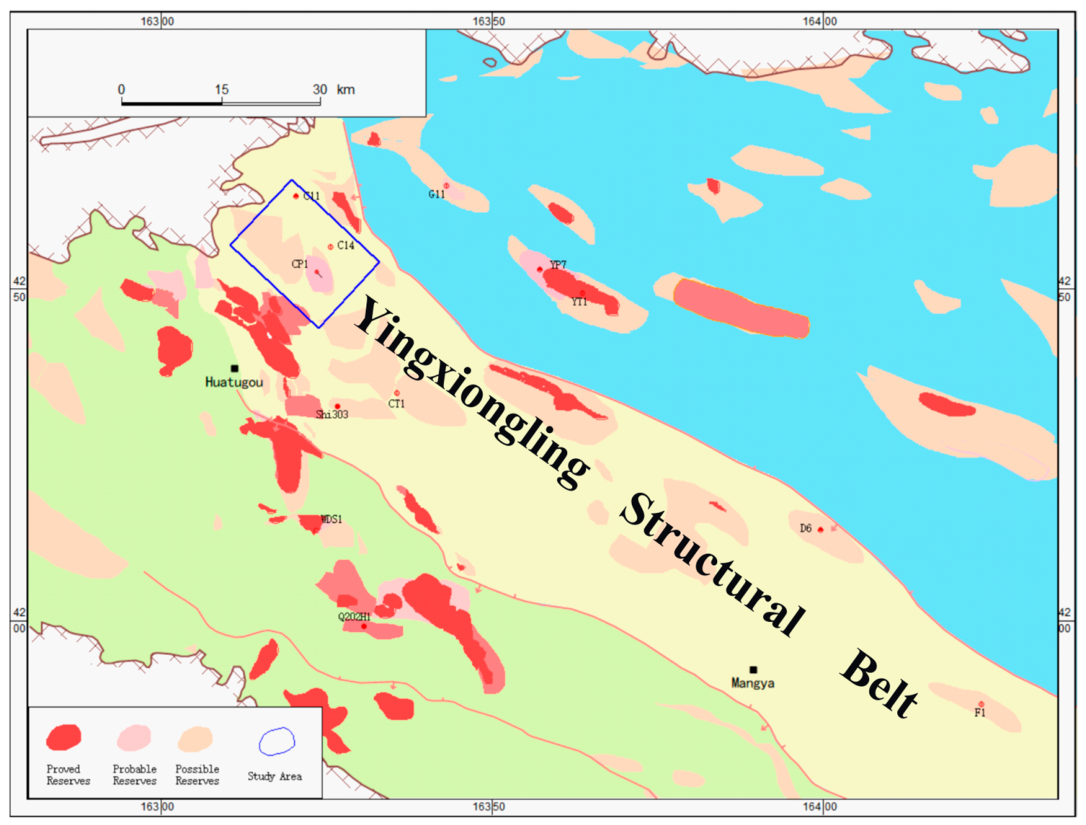
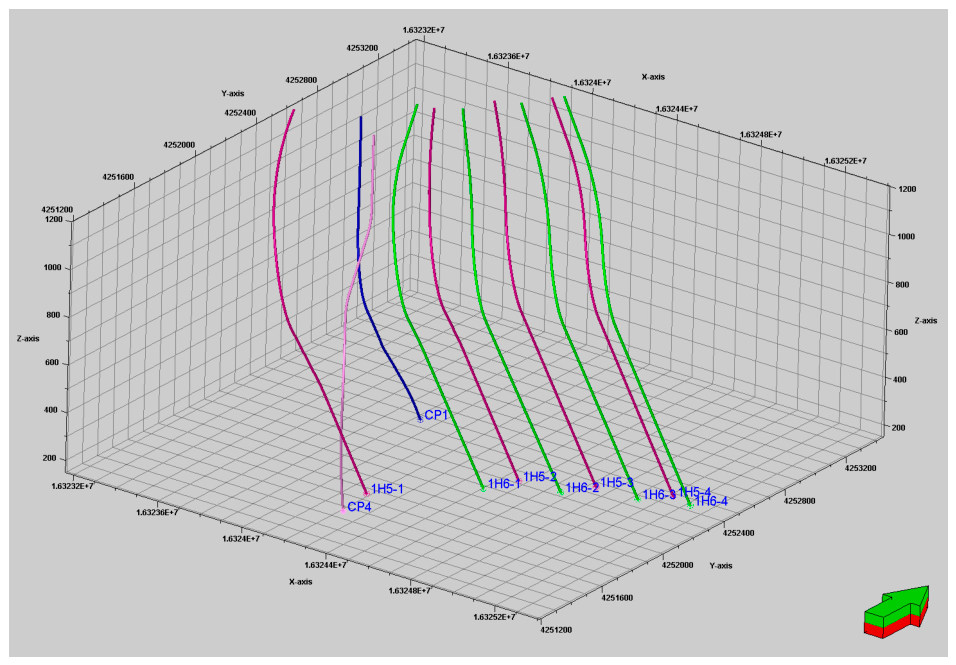
The study area is located in the central part of the Ganchai Valley structural belt within the Yingxiongling area, western Qaidam Basin (Figure 1). The 1H platform was designed to evaluate three-dimensional well-pattern parameters in a thick sweet-spot interval and to assess the productivity behavior of a horizontal-well group. The spatial distribution of platform wells and adjacent monitoring wells is shown in Figure 2. Wells 1H5-1 and 1H6-1 to 1H6-4 constitute the main well group of the 1H platform. Wells CP1 and CP4 are located on the north side of the platform, with horizontal distances of approximately 190 m and 210 m from the well group. They are used for production history calibration, geomechanical monitoring and inter-well tracer verification in this study. Both adjacent wells target the same Box 5–6 pay intervals of the Upper Member of Xiaganchaigou Formation (E₃²), with lateral lengths of 1520 m and 1480 m respectively, and have a production history of more than 2 years. The target interval is the E₃² Box 5 and Box 6 shale oil reservoir. The compact platform layout provides an appropriate field setting for studying platform-coordinated fracturing, tight spacing calibration and stress-interference effects [21,22,23].

2.2. Geological and Engineering Data Basis

Log-based statistics from 12 wells on the 1H platform, with a total of 1246 valid sample points (Box 5: 582 samples; Box 6: 664 samples), indicate that the average porosity, oil saturation and brittle-mineral content of Box 5 are 7.2%, 50.1% and 54.7%, respectively, whereas the corresponding values for Box 6 are 7.6%, 50.9% and 67.6% (

Table 1. Comparison of key geological and engineering parameters between Box 5 and Box 6 on the 1H platform.

Box	Porosity (%)	Oil Saturation (%)	Brittle Minerals (%)	GR (API)	RT (ohm·m)	Avg. Hydraulic Fracture Length (m)	Avg. Propped Fracture Length (m)
Box 5	7.2	50.1	54.7	86.2	12.0	172.64	150.93
Box 6	7.6	50.9	67.6	68.2	13.1	183.46	161.91

). Independent-samples t-test was used to analyze the statistical significance of the differences: porosity (p = 0.023 < 0.05), oil saturation (p = 0.031 < 0.05), and brittle-mineral content (p < 0.001) all show statistically significant differences. Although the absolute differences in porosity and oil saturation are relatively small, the 12.9-percentage-point difference in brittle-mineral content is the core factor leading to better fracability and fracture propagation capacity of Box 6. Compared with Box 5, Box 6 exhibits lower gamma-ray values, higher resistivity and higher brittle-mineral content, indicating better reservoir quality and higher fracability. Platform-scale fracture simulation further shows that the average hydraulic-fracture length and supported-fracture length in Box 6 are 183.46 m and 161.91 m, respectively, exceeding the corresponding values of 172.64 m and 150.93 m in Box 5 (Table 1).

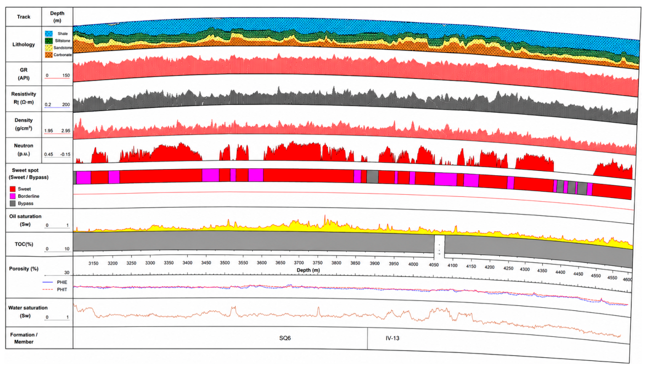
Well 1H6-1 is a representative well (Figure 3). The well has a total depth of 4606 m and a lateral length of 1500 m. Sweet spot classification criteria (logging thresholds): Class I sweet spot: GR < 70 API, RT > 12 Ω·m, porosity > 7.2%, oil saturation > 50%, brittle mineral content > 60%; Class II sweet spot: 70 ≤ GR ≤ 80 API, 11 ≤ RT ≤ 12 Ω·m, 7.0% < porosity ≤ 7.2%, 48% < oil saturation ≤ 50%, 55% < brittle mineral content ≤ 60%. After correction by LWD logging and conventional logs, the lateral section was drilled mainly within Box 6. The penetration ratio of Class I + II sweet spots reaches 90.6% with a measurement uncertainty of ±1.2%.

2.3. Workflow and Evaluation Indicators

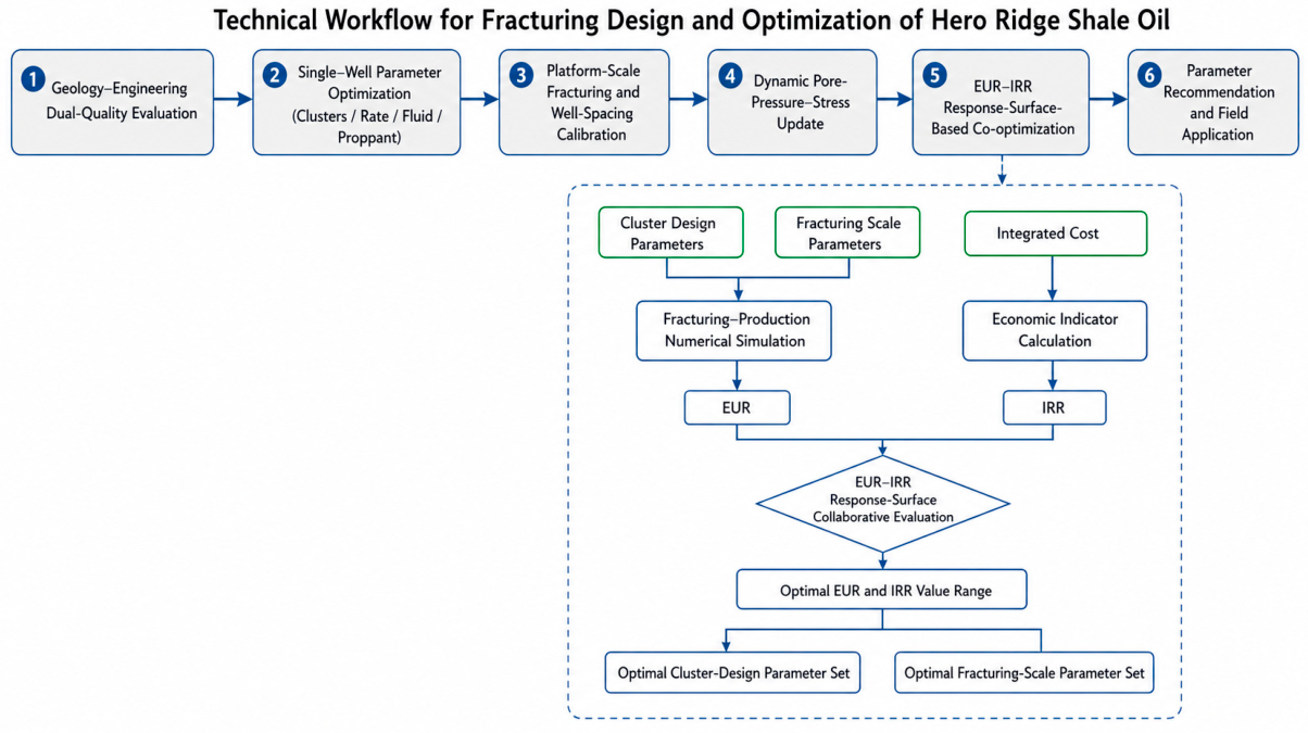
The proposed workflow integrates geology–engineering analysis with techno-economic evaluation (Figure 4). First, well logging, mud logging and three-dimensional geological models are jointly used to characterize reservoir quality and fracability, and to identify preferential stimulation intervals. Second, sensitivity analyses of cluster number, pumping rate, fluid intensity, and proppant intensity are conducted for representative wells to quantify their effects on fracture geometry and EUR response. Third, the single-well simulation results are extended to the platform scale by considering tight well-spacing, post-fracturing stress redistribution, and production-induced stress-field evolution. Finally, project cash-flow analysis and EUR-IRR results under different lateral-length and well spacing combinations are integrated to construct two-dimensional contour maps and three-dimensional normalized response surfaces for evaluating production scale, economic return and economically acceptable development ranges.

Well 1H6-1 was selected as the representative well because its lithology, petrophysical properties, in situ stress conditions, and brittleness are broadly consistent with the average characteristics of Boxes 5 and 6 on the 1H platform. For wells with lower sweet-spot penetration, the treatment scale should be adjusted by appropriately reducing fluid and proppant intensities.

Fracture numerical simulation was performed using Kinetix 2021 (Schlumberger, Houston, TX, USA) based on a discrete fracture network (DFN) model. Four-dimensional geomechanical simulation was conducted using Visage 2021 (Schlumberger, Houston, TX, USA) to evaluate pore-pressure evolution, stress redistribution, and inter-well interference during sequential fracturing and production.

Available field data, including microseismic interpretation, production-history matching, and tracer-response information, were used to constrain the simulation results. Because complete post-fracturing diagnostic data are not available for all wells, the simulation results are regarded as field-constrained numerical predictions rather than fully diagnostic validations.

The key input parameters and data sources are as follows:

(1)

Reservoir parameters, including reservoir thickness, porosity, and permeability, were derived from core measurements and well-log interpretation.

(2)

Rock mechanical properties and in situ stress parameters were obtained from core triaxial tests and field stress measurements.

(3)

Fracturing fluid properties, proppant parameters, and treatment design parameters were constrained by field operation data and engineering empirical estimates.

2.4. Key Evaluation Equations

This study adopts a nonlinear cost model to calculate drilling, completion and surface engineering investments. The model characterizes the nonlinear relationship between development costs and lateral length/well spacing and reduces the bias that may arise from a simple linear cost for long horizontal wells [37,38,39,40]. To establish a unified quantitative basis for fracturing-parameter optimization, lateral-length/well-spacing evaluation and economic assessment, the following equations are used to define EUR, net cash flow, NPV, IRR, normalized response and the integrated optimization objective.

EUR = Σ_{t = 1}^{T} q_{o,t} Δt

(1)

where q_{o,t} is the oil production rate or oil volume in time step t, Δt is the time-step length and T is the evaluation period. For different lateral-length and well-spacing combinations, EUR represents the cumulative production response of the corresponding development scheme.

NCF_t = P_t Q_t η − C_{op,t} − I_t − Tax_t

(2)

where NCF_t is net cash flow in year t, P_t is oil price, Q_t is annual oil production, η is the marketable-oil ratio, C_{op,t} is operating cost, I_t is investment and Tax_t is taxes and fees.

NPV(r) = Σ_{t = 0}^{T} NCF_t/(1 + r)^t

(3)

Σ_{t = 0}^{T} NCF_t/(1 + IRR)^t = 0

(4)

The IRR is the discount rate that makes the NPV equal to zero. A higher IRR indicates stronger cash-flow recovery capacity per unit investment and is controlled by production, investment intensity, operating cost, oil price and tax conditions.

EUR_n = (EUR − EUR_min)/(EUR_max − EUR_min)

(5a)

IRR_n = (IRR − IRR_min)/(IRR_max − IRR_min)

(5b)

Normalized variables EUR_n and IRR_n are used only for cross-index visualization in the same 3D space and do not alter the physical or economic meaning of the original values.

F(L,S) = w_E EUR_n(L,S) + w_I IRR_n(L,S)

(6)

where L is lateral length, S is well spacing, and w_E and w_I are weights assigned to production and economic responses. For balanced production-economic optimization, w_E = w_I = 0.5 is adopted in this study, which conforms to the general principle of “balancing production scale and investment return” in domestic shale oil development. When the development objective focuses on production capacity construction, w_E can be increased to 0.6–0.7; when focusing on investment recovery, w_I can be increased to 0.6–0.7.

max F(L,S), subject to IRR(L,S) ≥ i_0, L_min ≤ L ≤ L_max, S_min ≤ S ≤ S_max

(7)

In this study, i_0 is set to 6%, the minimum acceptable economic return for energy industry projects in China. Equation (7) expresses the core concept of coordinating EUR and IRR under an economic constraint.

3. Results

3.1. Cluster-Number Optimization

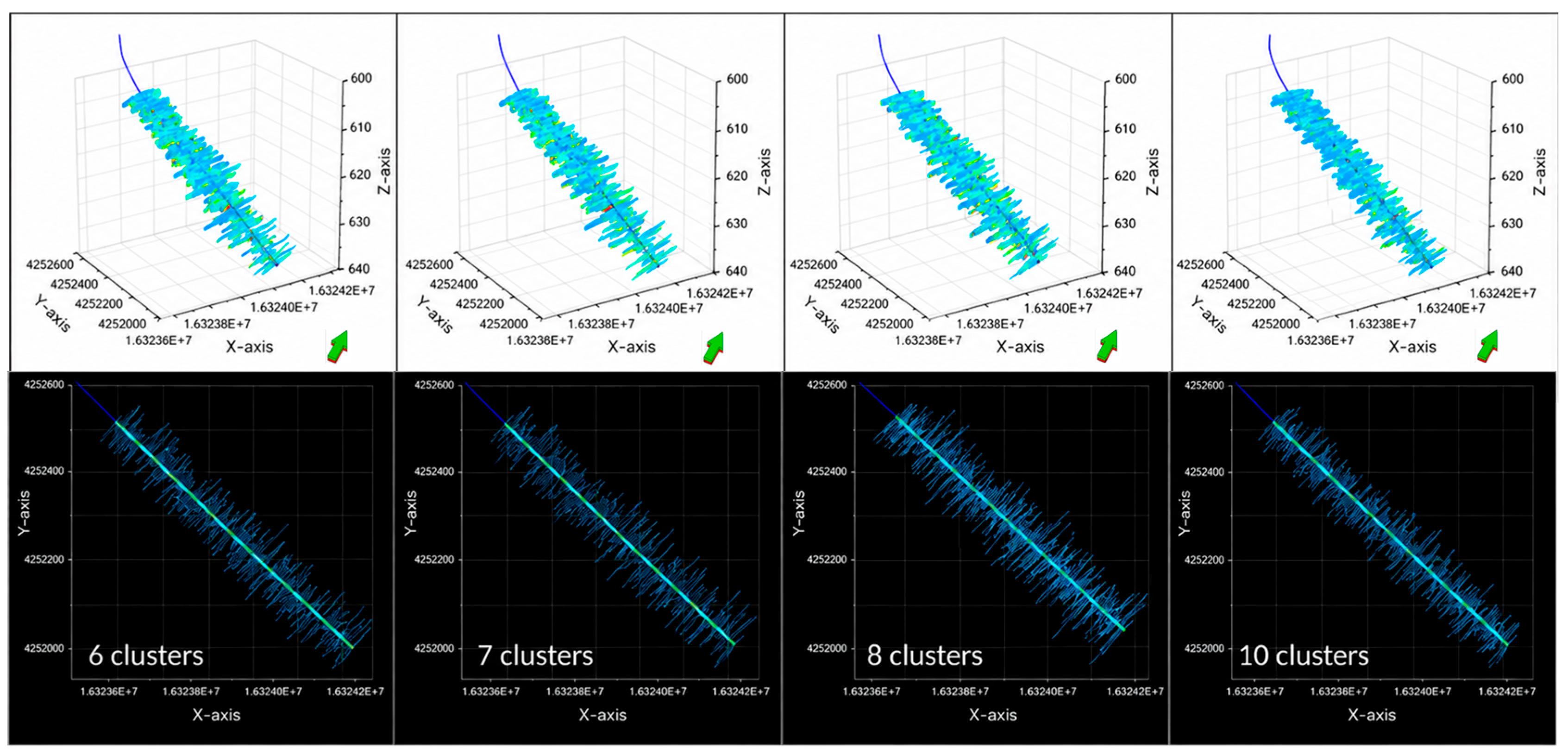
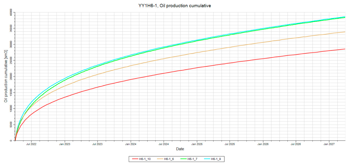
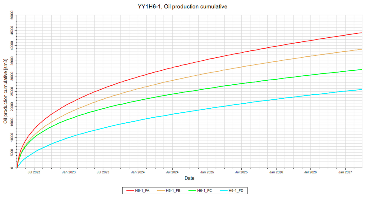
Cluster-number sensitivity was evaluated for Well 1H6-1 under fixed conditions: 18 m³/min pumping rate, 35 m³/m fluid intensity, 3.25 m³/m proppant intensity, and 48 total perforation holes. The six-, seven-, eight- and 10-cluster schemes were compared in terms of fracture morphology (Figure 5), fracture parameters (

Table 2. Fracture–parameter comparison for different cluster-number schemes of Well 1H6-1.

Clusters	Avg. In-Fracture Volume (m3)	Fluid Efficiency (%)	Hydraulic Network Length (m)	Propped Network Length (m)	Fracture Conductivity (mD·m)
6	581.40	28.344	151.64	133.92	235.96
7	607.28	29.604	166.96	148.12	235.28
8	674.48	32.880	185.16	164.32	305.04
10	489.56	23.860	135.92	112.12	144.92

) and production response (Figure 6). The eight-cluster scheme produced the most complex and uniform fracture distribution, with an average fracture volume of 674.48 m³, hydraulic fracture network length of 185.16 m, propped fracture network length of 164.32 m, and fracture conductivity of 305.04 mD·m (Table 2). Five-year production forecasts show that the differences between the seven- and eight-cluster schemes are relatively small, but the eight-cluster scheme delivers slightly higher five-year cumulative oil production. By contrast, the 10-cluster scheme yields a clearly lower EUR than the other schemes (Figure 6).

Post-fracturing microseismic monitoring of Well 1H6-1 indicates an average fracture half-length of 162 ± 15 m. This estimate is consistent with the simulated value of 164.32 m within the monitoring uncertainty, providing field-scale support for the adopted fracture model.

From an engineering operation perspective, the difference in single-stage construction time between the seven-cluster and eight-cluster schemes is about 15 min, and the difference in total single-well construction time is about 3 h, which has negligible impact on the overall project schedule. However, the five-year cumulative oil production of the eight-cluster scheme is 2.1% higher than that of the seven-cluster scheme. At the current oil price, this translates to an additional economic benefit of approximately RMB 1.2 million per well, which is much higher than the additional construction cost of one cluster (about RMB 150,000). In addition, the more uniform fracture distribution of the eight-cluster scheme can effectively reduce unproduced reservoir areas and lower the risk of inter-well interference in later stages. Therefore, the eight-cluster scheme is more advantageous from a comprehensive technical and economic perspective.

These results suggest that Yingxiongling shale oil is not suitable for blindly pursuing extremely dense cluster designs. Too few clusters leave unmodified areas between major fractures, whereas too many clusters intensify intra-stage stress shadowing and cluster competition, reducing far-field extension capability. The eight-cluster scheme provides a better balance between near-wellbore stimulation and far-field reservoir contact. From an economic perspective, the 10-cluster scheme does not convert additional completion complexity into higher EUR; therefore, the eight-cluster scheme is more reasonable overall [24,25,26].

3.2. Pumping-Rate Optimization

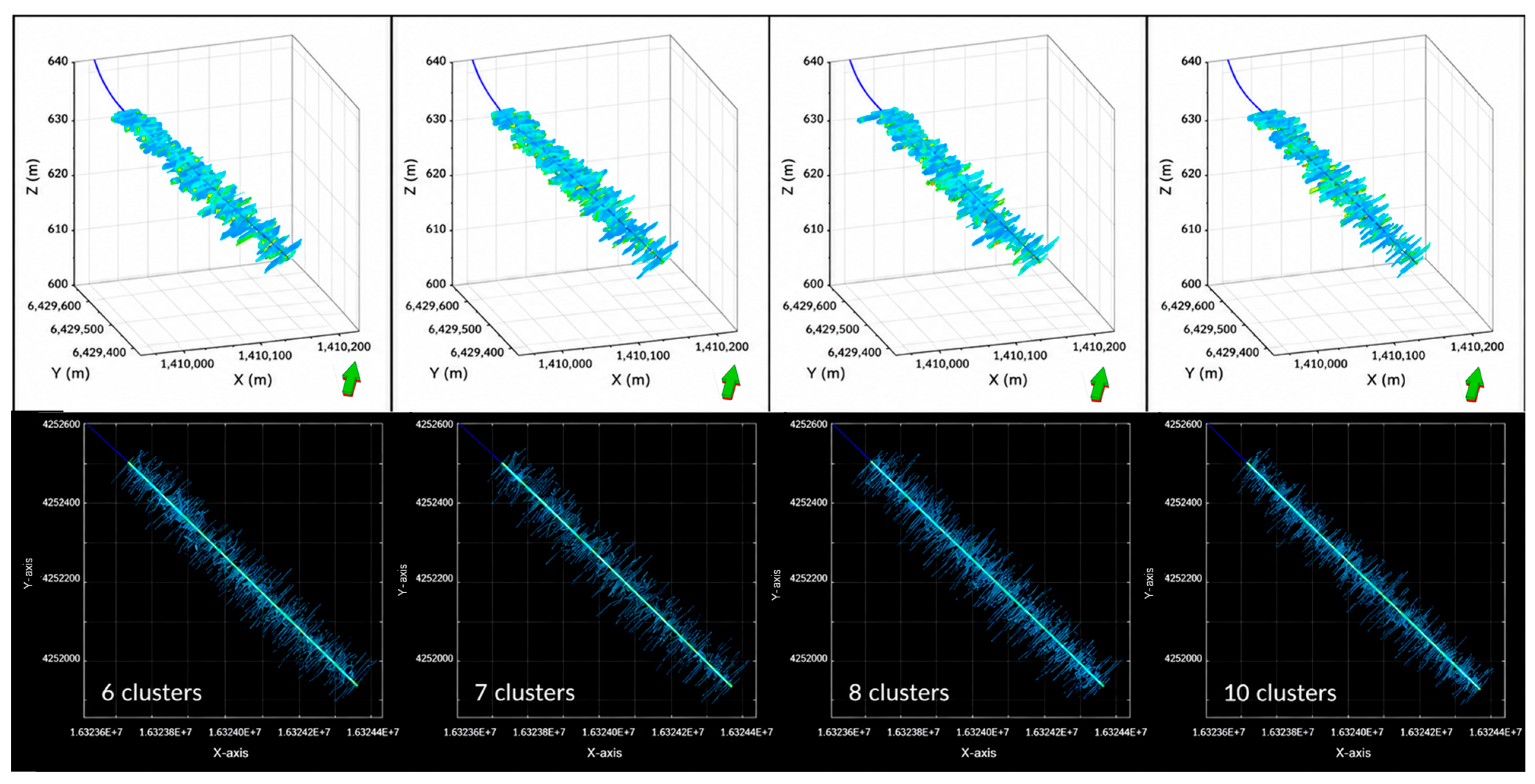
Under the eight-cluster, 35 m³/m fluid-intensity and 3.25 m³/m proppant-intensity conditions, pumping rates of 12, 14, 16 and 18 m³/min were compared. Average in-fracture volume, hydraulic fracture network length, and propped fracture network length generally increased with pumping rate. The 18 m³/min scheme had an average in-fracture volume of 571.44 m³, hydraulic-fracture-network length of 152.40 m and propped-fracture-network length of 133.48 m. Five-year forecasts show that the 18 m³/min scheme delivers significantly better EUR response than the lower-rate schemes (Figure 7;

Table 3. Fracture–parameter comparison for different pumping-rate schemes of Well 1H6-1.

Pumping Rate (m3/min)	Avg. In-Fracture Volume (m3)	Fluid Efficiency (%)	Hydraulic Network Length (m)	Propped Network Length (m)	Fracture Conductivity (mD·m)
12	462.56	22.536	139.84	118.24	191.40
14	535.52	26.108	140.60	122.04	217.88
16	551.00	26.860	146.00	124.04	251.96
18	571.44	27.852	152.40	133.48	203.84

).

For a conventional sweet-spot well dominated by Box 6, a higher pumping rate improves net pressure and fracture-extension capability, thereby increasing reservoir contact. However, a higher pumping rate is not universally optimal. In tight spacing platforms, excessive pumping rate may aggravate fracture overlap and inter-well stress interference. We therefore recommend 18 m³/min for conventional sweet-spot wells, but caution against applying this value directly to all well spacings and platform layouts.

3.3. Fluid-Intensity Optimization

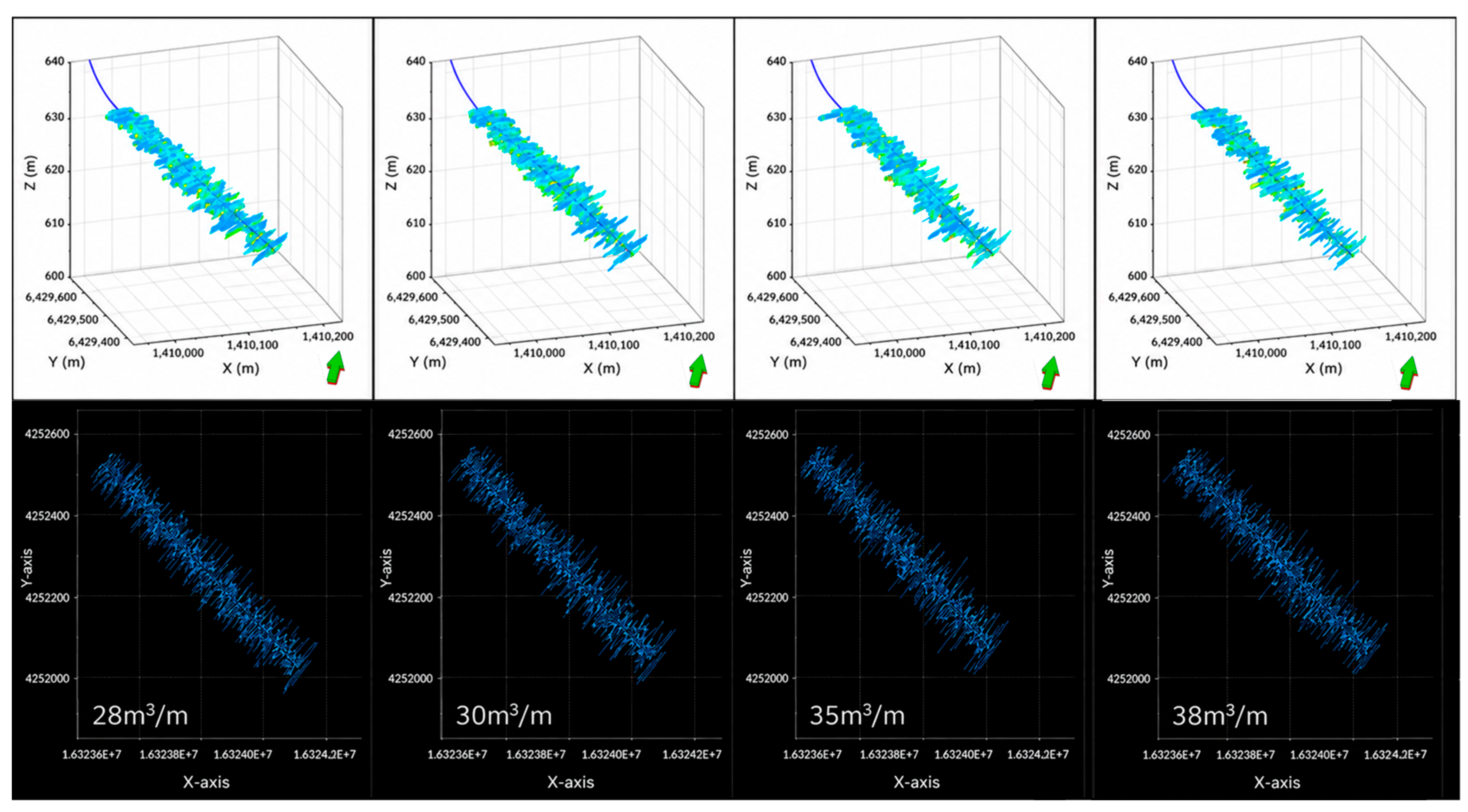
With eight clusters, a pumping rate of 18 m³/min and a proppant intensity of 3.25 m³/m, fluid intensities of 28, 30, 35 and 38 m³/m were compared. The fracture morphology and parameter responses are shown in Figure 8 and

Table 4. Fracture–parameter comparison for different fluid-intensity schemes of Well 1H6-1.

Fluid Intensity (m3/m)	Avg. In-Fracture Volume (m3)	Fluid Efficiency (%)	Hydraulic Network Length (m)	Propped Network Length (m)	Fracture Conductivity (mD·m)
28	471.04	25.996	149.92	129.76	179.16
30	541.44	28.028	150.00	130.72	219.44
35	603.00	27.024	156.20	139.84	202.76
38	632.84	26.232	164.32	139.76	197.84

, and the corresponding production forecast is presented in Figure 9. Increasing fluid intensity continuously increases average fracture volume, hydraulic-fracture-network length and propped-fracture-network length and makes the fracture pattern more complex. However, the differences between the 35 and 38 m³/m schemes become much smaller, and the production forecast indicates only a limited EUR increment when fluid intensity is increased from 35 to 38 m³/m (Figure 9). Considering both fracture parameters and production response, 35 m³/m is the preferred fluid intensity.

From a techno-economic perspective, fluid-intensity increases before 35 m³/m substantially improve fracture volume and reservoir-control extent; when intensity is further increased to 38 m³/m, the marginal EUR gain becomes limited while the input scale continues to increase. Because IRR is sensitive to both production realization and marginal cost, 35 m³/m is more reasonable than further increasing fluid intensity.

3.4. Proppant Intensity and Proppant-System Optimization

For Well 1H6-1, proppant intensities of 2.8, 3.0, 3.25 and 3.5 m³/m were compared. The differences in fracture geometry among the schemes are relatively limited, but the production responses associated with 3.25 and 3.5 m³/m are more favorable. After considering incremental economic cost, 3.25 m³/m is recommended. The recommended parameter windows for conventional sweet-spot wells and 200 m-spaced wells are summarized in

Table 5. Recommended parameter windows for conventional wells and 200 m-spaced wells in Yingxiongling.

Condition	Clusters per Stage	Pumping Rate (m3/min)	Fluid Intensity (m3/m)	Proppant Intensity	Prepad Fluid	Proppant System
Conventional sweet-spot well	8 clusters	18	35	3.25 m3/m	High-viscosity gel ~200 m3	70/140 + 40/70 mesh quartz sand, with 30/50 mesh ceramic tail-in
200 m-spaced well	Differential design	16	32	3.125 m3/m	Gel ~100 m3	Matched design to control fracture overlap and inter-well interference

. Results from Well CP4 further indicate that proppant optimization should consider not only total proppant volume but also proppant system design and pumping schedule. A prepad of approximately 200 m³ of high-viscosity gel increases single-well EUR by approximately 5.6% compared with the full slickwater scheme, and a proppant combination dominated by 70/140 mesh and 40/70 mesh quartz sand with 30/50 mesh ceramic tail-in for near-wellbore packing performs better.

3.5. Parameter Correction and Dynamic Stress Response Under Tight Well Spacing

Wells 1H6-3 and 1H6-4 were tested with 200 m spacing. Simulations show that, for tight spacing wells, the operating parameters should be adjusted to a pumping rate of 16 m³/min, fluid intensity of 32 m³/m and proppant intensity of 3.125 m³/m, with 100 m³ of prepad gel (Table 5). This parameter set reduces fracture length and overlap and better matches fracture scale with 200 m well spacing. Directly applying the high-rate and high-fluid-volume scheme designed for conventional wells may increase single-well fracture size, but it can also intensify inter-well stress interference and fracture overlap, thereby reducing platform-level reservoir contact efficiency.

Four-dimensional geomechanical simulation was performed using Visage 2021 (Schlumberger, Houston, TX, USA) to evaluate pore-pressure/stress coupling during fracturing and production. The model was constrained by heterogeneous rock-mechanical properties derived from well logs and core tests, and the updated pore-pressure and stress fields were then imposed on adjacent-well fracture simulations.

(1)

Basic assumptions: The reservoir rock is an elastic–plastic medium, and the Mohr-Coulomb yield criterion is adopted. Hydraulic fractures are treated as high-permeability channels with permeability increased by three orders of magnitude after fracturing.

(2)

Boundary conditions: The top of the model is a free surface, the bottom is a fixed displacement boundary, and the sides are normal constraint boundaries.

(3)

Coupling and stress updating method: A stepwise coupling algorithm was used: (1) At each production time step (3 months), the change in pore pressure field was calculated first; (2) The pore pressure change was input as a load to calculate the redistribution of effective stress field; (3) Rock mechanical parameters (Young’s modulus, Poisson’s ratio) were updated for subsequent fracture simulation of adjacent wells.

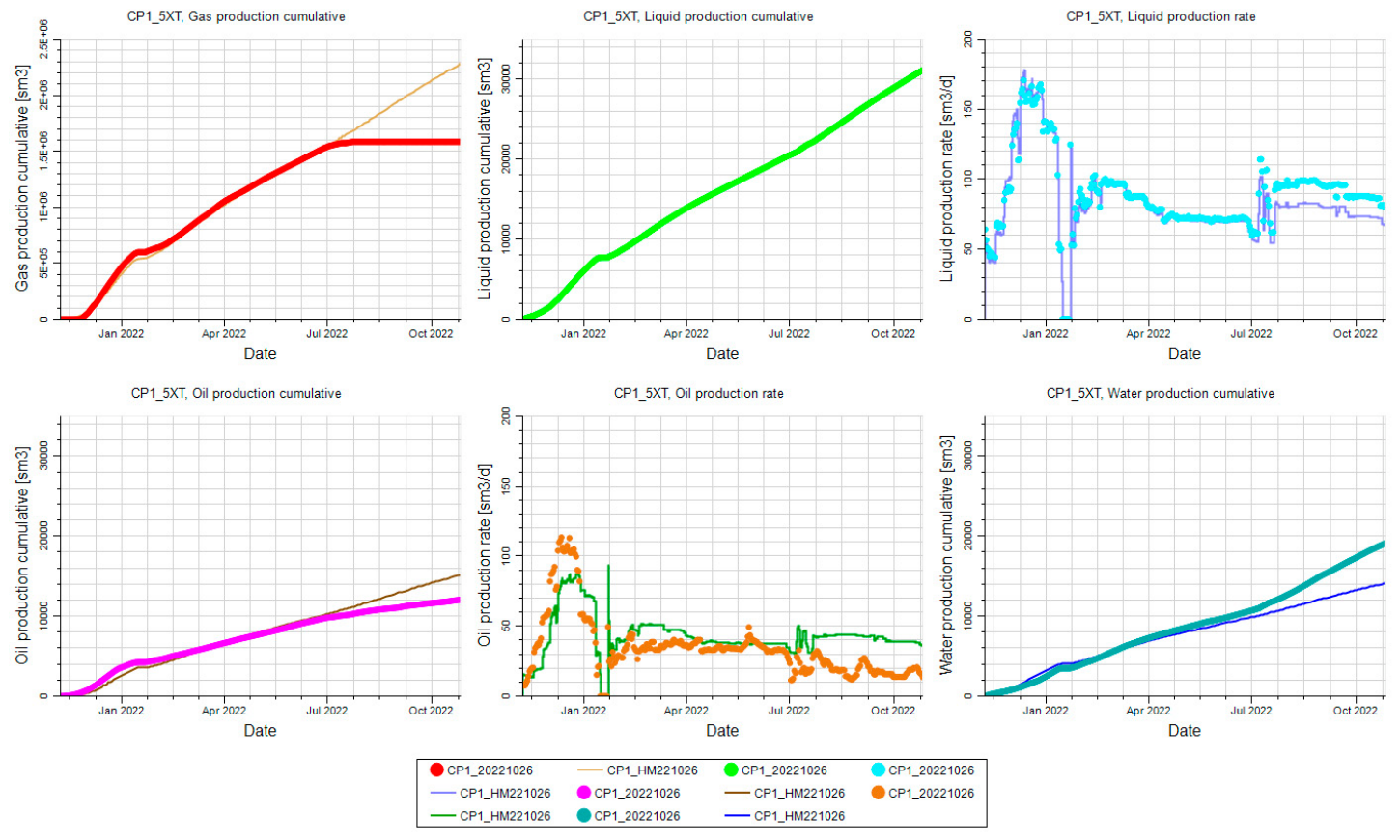
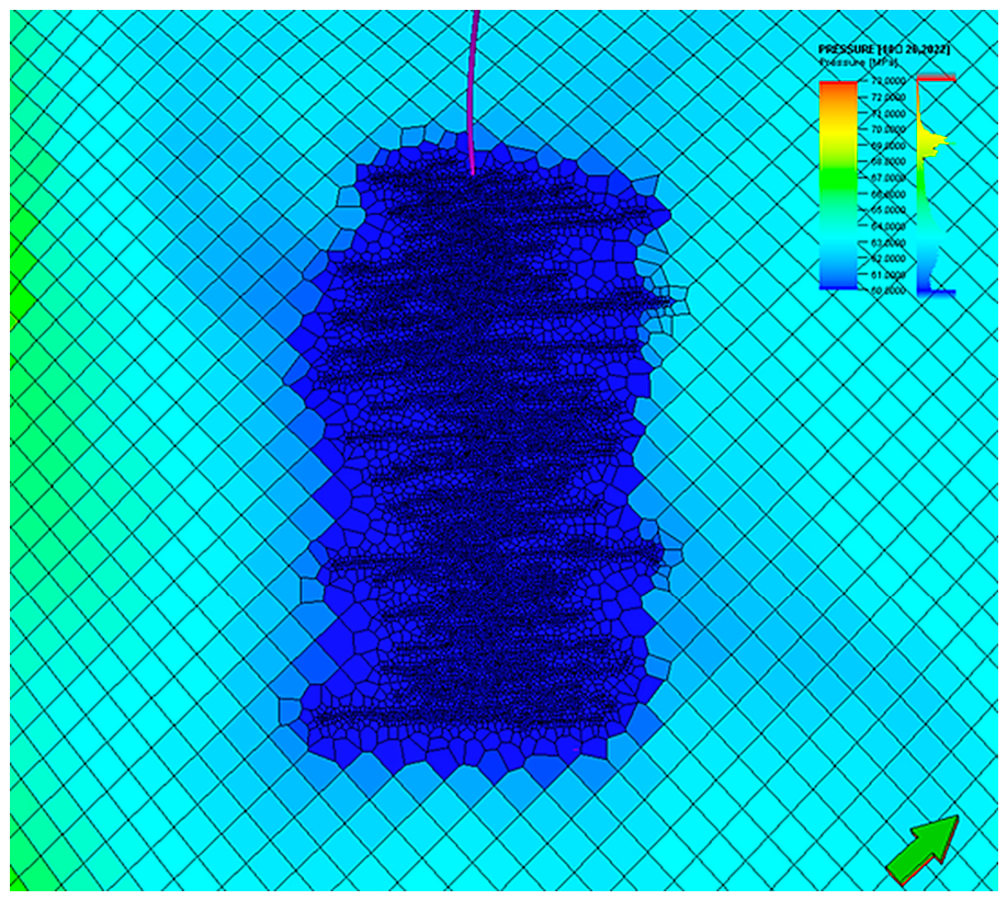
Four-dimensional geomechanical simulation for Well CP1 indicates that the minimum horizontal principal stress near the wellbore increases by approximately 6–10 MPa after fracturing, and stress and pore-pressure perturbations persist even after partial relaxation during production. Production-history matching and post-fracturing pore-pressure response are shown in Figure 10 and Figure 11. When the updated pore-pressure and stress fields are imposed on adjacent-well fracture simulations, fracture propagation directions are deflected, and partial fracture communication risk increases. Therefore, platform fracturing design should incorporate post-fracturing and post-production dynamic stress updating into subsequent-well design.

Integrated interpretation of microseismic monitoring and inter-well tracer data from Wells CP1 and CP4 indicates a single-side stress-influence range of 125–165 m for Box 5 and Box 135–170 m for Box 6, which is broadly consistent with the Visage-simulated stress-disturbance range. Tracer monitoring from adjacent Well CP1 shows differentiated activation among reservoir lithofacies: laminated intervals respond earlier under relatively low drawdown, whereas more massive dolomitic intervals require higher drawdown before becoming fully active. The attenuation of tracer signals in some intervals during later production suggests stress-sensitive fracture conductivity, supporting the need for dynamic stress updating in tight-spacing platform development.

4. EUR-IRR Analysis and Lateral-Length/Well Spacing Optimization

4.1. Economic-Evaluation Boundary

The expanded pilot scheme includes 24 horizontal wells. Economic calculations were based on the nonlinear cost model and a 1-year construction plus 14-year operation period. Short-term production forecasts were combined with Arps decline extrapolation to estimate the 15-year EUR. The major economic-evaluation results are summarized in

Table 6. Key economic-evaluation results of the expanded pilot-development scheme.

Indicator	Value	Remark
Total investment	RMB 1299.82 million	Excluding taxes
Construction investment	RMB 1261.24 million	Drilling, production engineering and surface facilities
Construction-period interest	RMB 20.89 million	Effective loan rate 4.14%
Working capital	RMB 17.69 million	30% equity and 70% loan
Single-well investment	RMB 54.16 million	Average for 24 horizontal wells
Total project EUR	36.45 × 104 t	Converted from 42.38 × 104 m3, crude density = 0.86 t/m3
After-tax NPV	RMB 326.52 million	Benchmark return rate 6%, 15-year evaluation period
After-tax financial IRR	12.5%	Overall IRR of the recommended scheme
Payback period	4.82 years	Static investment recovery period

.

The project cash-flow model uses a 1-year construction period and 14-year operating period. Key economic parameters and their justifications are as follows:

(1)

Oil price: A stepped price of 50 USD/bbl for 2023–2024 and 60 USD/bbl thereafter, consistent with the benchmark scenario in CNPC’s 2023–2030 Oil and Gas Price Forecast Report.

(2)

Taxation: 13% value-added tax based on the Interim Regulations on Value-Added Tax of the People’s Republic of China; 5.8% resource tax based on the Resource Tax Law of the People’s Republic of China and Qinghai Province’s preferential oil and gas resource tax policy.

(3)

Financing structure: a 20% equity and 80% bank-loan ratio was adopted according to the financing practice of domestic shale oil development projects and relevant economic-evaluation specifications.

(4)

Benchmark return rate: 6% financial benchmark return rate, specified in the Methods and Parameters for Economic Evaluation of Construction Projects (3rd Edition) for energy industry projects.

(5)

Operating cost: Derived from actual operation data of the Yingxiongling shale oil project from 2022 to 2023.

The marketable-oil ratio is 98.96%, and the annual loan interest rate is 4.14%, the actual rate for long-term construction loans for oil and gas projects in China.

4.2. Coupling Relationship Between Parameter Optimization and Economics

Under the project-level economic boundary and nonlinear cost framework, the recommended pilot scheme yields an after-tax IRR of 12.5%, an after-tax NPV of RMB 326.52 million and an after-tax static payback period of 4.82 years (Table 6). The sensitivity analysis (

Table 7. Results of IRR sensitivity analysis.

Scenario	IRR (%)	Change Relative to Base Case (pct)
Base case	12.50	0.00
Oil price −10%	8.85	−3.65
Production −10%	8.87	−3.63
Investment +10%	9.79	−2.71
Cost +10%	11.75	−0.75
Production +10%	16.04	+3.54
Oil price +10%	16.06	+3.56

) indicates that oil price and production exert the strongest control on IRR, followed by investment and operating cost. Therefore, EUR improvement translates into IRR only when incremental production is sufficient to offset the additional investment. This supports the need for EUR-IRR co-evaluation of lateral length and well spacing.

4.3. EUR-IRR Response Under Lateral-Length and Well Spacing Combinations

To evaluate the combined influence of lateral length and well spacing on production scale and economic return, the original 45 groups of parameter combinations were screened before response-surface construction. Redundant and repeated gradient points were removed, and 27 representative schemes were retained. These schemes cover the main engineering ranges considered in this study and preserve the characteristic trends of both EUR and IRR. The Ordinary Kriging interpolation method was then used to construct the EUR-IRR response surfaces.

(1)

Data preprocessing: Outlier elimination and unit unification were performed on the full-gradient discrete field data in

Table 8. Representative EUR and IRR data under different lateral-length and well-spacing combinations.

Lateral Length (m)	Well Spacing (m)	EUR (104 m3)	IRR (%)
500	50	7.82	−32.5
500	600	2.21	−65.1
1000	50	14.76	−5.3
1000	100	12.35	−12.8
1000	150	10.68	−19.1
1000	600	3.57	−51.3
1500	50	22.15	2.8
1500	100	18.79	−2.7
1500	600	5.48	−38.7
2000	50	29.87	7.5
2000	300	14.72	−11.8
2000	600	7.56	−30.2
3000	50	45.62	10.2
3000	100	42.78	7.2
3000	150	37.15	3.8
3000	200	32.48	0.9
3000	300	24.96	−4.1
3000	600	12.87	−19.5
4000	50	59.87	11.5
4000	100	56.63	10.8
4000	150	49.32	8.7
4000	200	43.15	6.4
4000	300	33.28	2.1
4000	600	17.15	−9.8
5000	50	72.15	5.8
5000	300	40.89	−4.8
5000	600	21.08	−15.6

.

(2)

Variogram fitting: The spherical model was used to fit the experimental variogram, with a nugget value of 0.05, sill value of 0.92, and range of 800 m.

(3)

Grid generation: A 50 m × 50 m regular grid was created covering lateral lengths of 500–5000 m and well spacings of 50–600 m.

(4)

Response surface smoothing: Cubic spline smoothing was applied to eliminate interpolation noise, with a smoothing coefficient of 0.8.

(5)

Normalization processing: EUR and IRR were normalized according to Equations (5a) and (5b) to generate the 3D optimization map.

Cross-validation results show that the root mean square error (RMSE) is 4.2% for EUR interpolation and 5.7% for IRR interpolation. In the data-constrained solution region (3500–4000 m lateral length and 150–200 m well spacing), the errors are less than 3%, indicating acceptable interpolation reliability within this region.

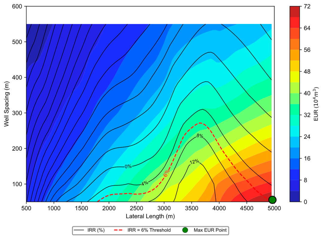
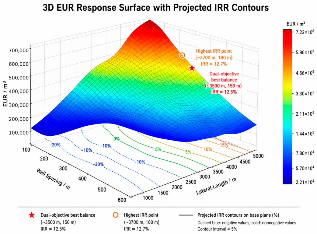
The integrated two-dimensional EUR-IRR contour map and the three-dimensional EUR response surface with projected IRR contours are shown in Figure 12 and Figure 13, respectively. The results show that EUR generally increases with longer lateral length and smaller well spacing, whereas IRR does not vary synchronously with EUR. Excessively small spacing increases well count, total drilling completion investment, and inter-well stress interference; therefore, some high EUR schemes show weak economic performance (Figure 12; Table 8).

During response-surface construction and 3D visualization (Figure 12 and Figure 13), EUR and IRR were normalized using Equations (5a) and (5b). The threshold of IRR ≥ 6% defined in Equation (7) was adopted to divide economically acceptable regions. High-EUR schemes that fail to meet this economic constraint are classified as production-potential zones rather than recommended development schemes.

Based on the response-surface results, the maximum EUR of 721,500 m³ is obtained at a lateral length of 5000 m and a well spacing of 50 m, with a corresponding IRR of only 5.8%. The maximum IRR of 12.7% appears at a lateral length of 3700 m and a well spacing of 180 m, with an EUR of 456,200 m³ (Figure 12 and Figure 13). A field-recommended balanced scheme is selected at 3500 m lateral length and 150 m well spacing, with an EUR of 423,800 m³ and an IRR of 12.5%. These results indicate that production gain and economic return are partially decoupled under the present cost structure.

To analyze the influence of weighting coefficients on optimal development strategies, we consider:

(1) Production-oriented scenario (w_E = 0.7, w_I = 0.3): Optimal scheme: 4000 m lateral length + 200 m well spacing, EUR = 43.15 × 10⁴ m³, IRR = 6.4%.

(2) Balanced scenario (w_E = 0.5, w_I = 0.5): Optimal scheme: 3500 m lateral length + 150 m well spacing, EUR = 42.38 × 10⁴ m³, IRR = 12.5%.

(3) Economic-oriented scenario (w_E = 0.3, w_I = 0.7): Optimal scheme: 3700 m lateral length + 180 m well spacing, EUR = 45.62 × 10⁴ m³, IRR = 12.7%.

The results indicate that the weighting coefficient mainly affects the optimal well spacing, while the optimal lateral length is stably maintained within the range of 3500–4000 m. This conclusion provides flexible parameter selection options for different development priorities.

To verify the robustness of the EUR-IRR response surface under economic uncertainty, sensitivity analysis of ±10% oil price fluctuation was extended to the whole lateral-length–well-spacing parameter space.

When the oil price decreases by 10%, the IRR ≥ 6% economically acceptable zone shrinks overall: the boundary shifts toward wider well spacing and longer lateral length, and the maximum IRR point moves slightly to the direction of larger well spacing. When the oil price increases by 10%, the economically acceptable zone expands significantly, and schemes with smaller well spacing also meet the economic threshold.

Under both ±10% oil-price scenarios, the recommended balanced scheme (3500 m lateral length, 150 m well spacing) remains above the 6% economic threshold. Its IRR decreases to 8.85% when the oil price declines by 10% and increases to 16.06% when the oil price rises by 10%, indicating robust economic feasibility within the tested price range.

5. Discussion

The key issue in Yingxiongling shale oil fracturing is not a local optimum of a single parameter, but a coordinated optimum under the combined constraints of reservoir quality, engineering quality, well spacing, lateral length, dynamic stress field and economic return. Box 6 has better reservoir quality and fracture-extension performance than Box 5, confirming the importance of stratigraphic selection. The eight-cluster, 18 m³/min, 35 m³/m and 3.25 m³/m combination for Well 1H6-1 indicates that medium-to-high stimulation intensity is favorable for effective reservoir control under high-quality sweet-spot conditions.

The lateral-length and well-spacing response-surface analysis further shows that high-EUR schemes are mainly concentrated in longer laterals and smaller well spacings. These schemes require higher investment and may intensify inter-well interference, leading to reduced IRR. In this study, the maximum EUR is obtained at 5000 m lateral length and 50 m spacing, whereas the maximum IRR occurs at 3700 m lateral length and 180 m spacing. This difference confirms that the production optimum and the economic optimum are not the same, a feature commonly observed in tight-oil and shale oil development [38].

The main implication is that fracturing optimization should not be limited to maximizing single-well or platform EUR. IRR also cannot be discussed independently of fracture propagation, well-pattern control, and reservoir-contact mechanisms. A rational workflow should be built on a closed loop of geological sweet-spot selection, engineering-parameter matching, platform well-pattern coordination, lateral-length/well-spacing optimization, and project economic acceptability. The EUR-IRR response-surface analysis developed in this study provides a practical bridge between simulation-based technical optimization and project-level economic decision-making.

This study has several limitations. First, the EUR-IRR response surfaces were constructed from discrete scheme data and interpolation; therefore, uncertainty remains in regions with sparse data support, especially near the boundary of the parameter space. The recommended schemes are located mainly in the data-constrained region of 3500–4000 m lateral length and 150–200 m well spacing, where the interpolation error is relatively small. The response-surface-level economic sensitivity under oil price fluctuation (Figure S1) proves that the recommended scheme has good robustness within a reasonable parameter range. However, the economic model still simplifies some field variables, including service-cost fluctuation, operation duration, surface-facility adaptability, taxes, and financing conditions. Future work should incorporate more scheme data and additional operational variables to build a more detailed multi-parameter model linking incremental cost, incremental EUR, and incremental IRR.

6. Conclusions

(1)

The E₃² Box 5–6 shale oil reservoir on the Yingxiongling 1H platform shows clear inter-box differences. Box 6 is superior to Box 5 in porosity, oil saturation, brittle-mineral content and fracture-extension capacity, and is the preferred stimulation interval.

(2)

Single-well parameter optimization for Well 1H6-1 shows that the eight-cluster scheme is superior to the six-, seven- and 10-cluster schemes. For conventional sweet-spot wells, the optimized parameter combination is 18 m³/min pumping rate, 35 m³/m fluid intensity and 3.25 m³/m proppant intensity.

(3)

For 200 m-spaced wells, the fracturing parameters should be adjusted to 16 m³/min pumping rate and 32 m³/m fluid intensity, with 100 m³ of prepad gel. This reduces fracture overlap and inter-well stress interference and shifts the design logic from single-well optimum to platform-scale optimum.

(4)

Dynamic stress updating after fracturing and production has a significant impact on the subsequent fracture propagation of adjacent wells. The minimum horizontal principal stress near Well CP1 increases by 6–10 MPa after fracturing, and adjacent-well fracture direction and connection risk are strongly controlled by the updated pore-pressure-stress field.

(5)

Under the project-level economic boundary and nonlinear cost framework, the expanded pilot scheme has an after-tax IRR of 12.5%, an after-tax NPV of RMB 326.52 million, and a payback period of 4.82 years. The highest EUR is 721,500 m³ at 5000 m lateral length and 50 m well spacing (IRR = 5.8%). The maximum IRR reaches 12.7% at 3700 m lateral length and 180 m well spacing (EUR = 456,200 m³). The field-recommended balanced scheme at 3500 m lateral length and 150 m well spacing is recommended for field application.

(6)

This study presents a geology–engineering–economics integrated workflow for continental shale oil fracturing optimization. By coupling dynamic stress updating, platform-scale parameter correction, and EUR-IRR response-surface analysis, the workflow provides a practical quantitative basis for balancing production scale and investment return in highly heterogeneous shale oil reservoirs.

References

1. Sun, H.; Wang, H.; Yang, Y.; Lyu, Q.; Zhang, F.; Liu, Z.; Lyu, J.; Chen, T.; Jiang, T.; Zhao, P.; et al. Iteration and evaluation of shale oil development technology for continental rift lake basins. Pet. Explor. Dev. 2024, 51, 993–1008. [Google Scholar] [CrossRef] [Scilit]
2. Liu, H.; Kuang, L.; Su, J.; Meng, S.; Wei, X.; Wang, H.; Lei, Q.; Guo, J.; Jia, C.; Li, D. Practice and development suggestions of hydraulic fracturing technology in the Gulong shale oil reservoirs of Songliao Basin, NE China. Pet. Explor. Dev. 2023, 50, 688–698. [Google Scholar] [CrossRef] [Scilit]
3. Tang, H.; Luo, S.; Liang, H.; Zeng, B.; Zhang, L.; Zhao, Y.; Song, Y. Integrated numerical simulation of hydraulic fracturing and production in shale gas well considering gas-water two-phase flow. Pet. Explor. Dev. 2024, 51, 684–696. [Google Scholar] [CrossRef] [Scilit]
4. Zhu, Q.; Xiong, W.; Weng, D.; Li, S.; Guo, W.; Zhang, X.; Xiao, Y.; Luo, Y.; Fan, M. Theory and practice of energy-focused fracturing development technology. Pet. Explor. Dev. 2025, 52, 746–758. [Google Scholar] [CrossRef] [Scilit]
5. Yan, D.; Zhao, L.; Song, X.; Tang, J.; Zhang, F. Fracability evaluation model for unconventional reservoirs: From the perspective of hydraulic fracturing performance. Int. J. Rock Mech. Min. Sci. 2024, 181, 105912. [Google Scholar] [CrossRef] [Scilit]
6. Tang, H.; Ruan, Q.; Zhang, L.; Hu, D.; Qin, J.; Zhao, Y.; Ye, Y. Intelligent optimization of fracturing stage and cluster parameters for tight oil reservoir. Petroleum 2025, 11, 135–149. [Google Scholar] [CrossRef] [Scilit]
7. Ibrahim, A.F. Optimizing cluster spacing in multistage hydraulically fractured shale gas wells: Balancing fracture interference and stress shadow impact. J. Pet. Explor. Prod. Technol. 2024, 14, 2297–2313. [Google Scholar] [CrossRef] [Scilit]
8. Ju, Y.; Song, J.; Wang, Y. Stress shadow effects in multistage horizontal hydrofracturing of tight reservoirs: A numerical analysis considering perforation cluster spacings and fracturing sequences. Geomech. Geophys. Geo-Energy Geo-Resour. 2024, 10, 183. [Google Scholar] [CrossRef] [Scilit]
9. Shan, Q.; Mu, L.; Yuan, L.; Ji, Z.; Cheng, X.; Luan, H.; Jiang, Y.; Xun, W. Investigating multi-cluster hydraulic fracture propagation in tight reservoir considering actual perforation geometry. Geomech. Geophys. Geo-Energy Geo-Resour. 2025, 11, 69. [Google Scholar] [CrossRef] [Scilit]
10. Zhang, X.; Zhang, S.; Zou, Y.; Jia, H.; Li, J.; Wu, S. Fracture propagation characteristics of layered shale oil reservoirs with dense laminas under cyclic pressure shock fracturing. Geomech. Geophys. Geo-Energy Geo-Resour. 2024, 10, 154. [Google Scholar] [CrossRef] [Scilit]
11. Helmy, A.G.; Salem, S.K.; Elnoby, M. Sensitivity analysis of hydraulic fracturing parameters for optimum horizontal well spacing in tight oil reservoirs. Arab. J. Sci. Eng. 2025, 50, 4813–4832. [Google Scholar] [CrossRef] [Scilit]
12. Niu, W.; Lu, J.; Sun, Y.; Zhang, X.; Li, Q.; Cao, X.; Liang, P.; Zhan, H. Techno-economic integration evaluation in shale gas development based on ensemble learning. Appl. Energy 2024, 357, 122486. [Google Scholar] [CrossRef] [Scilit]
13. Niu, W.; Lu, J.; Sun, Y.; Mu, Y.; Zhang, J.; Guo, W.; Liu, Y. A Novel Framework Combining Production Evaluation and Quantification of Development Parameters for Shale Gas Wells. Geoenergy Sci. Eng. 2023, 226, 211752. [Google Scholar] [CrossRef] [Scilit]
14. Li, W.; Zhang, T.; Liu, X.; Dong, Z.; Dong, G.; Qian, S.; Yang, Z.; Zou, L.; Lin, K.; Zhang, T. Machine Learning-Based Fracturing Parameter Optimization for Horizontal Wells in Panke Field Shale Oil. Sci. Rep. 2024, 14, 6046. [Google Scholar] [CrossRef] [Scilit] [PubMed]
15. Ma, C.; Wu, H.; Luo, P.; Xu, P. A New Fracture Parameter Optimization Method for the Horizontal Well Section of Shale Oil. Front. Earth Sci. 2022, 10, 895382. [Google Scholar] [CrossRef] [Scilit]
16. Zhou, Q.; Dai, R.; Chen, L.; Wu, C.; Luo, S. Optimization of Refracturing Timing in Tight Oil Reservoirs Based on an Oil-Water Two-Phase Flow Model. Sci. Rep. 2025, 15, 22907. [Google Scholar] [CrossRef] [Scilit] [PubMed]
17. Bello, K.; Vikara, D.; Sheriff, A.; Viswanathan, H.; Carr, T.; Sweeney, M.; O’Malley, D.; Marquis, M.; Vactor, R.T.; Cunha, L. Evaluation of the Economic Implications of Varied Pressure Drawdown Strategies Generated Using a Real-Time, Rapid Predictive, Multi-Fidelity Model for Unconventional Oil and Gas Wells. Gas Sci. Eng. 2023, 113, 204972. [Google Scholar] [CrossRef] [Scilit]
18. Yan, B.; Liu, H.; Peng, X. Scenario analysis to evaluate the economic benefits of tight oil resource development in China. Energy Strategy Rev. 2024, 51, 101318. [Google Scholar] [CrossRef] [Scilit]
19. Cipolla, C.L.; Lolon, E.P.; Mayerhofer, M.J.; Warpinski, N.R. Fracture Design Considerations in Horizontal Wells Drilled in Unconventional Gas Reservoirs. In Proceedings of the SPE Hydraulic Fracturing Technology Conference, The Woodlands, TX, USA, 19–21 January 2009. SPE-119366-MS. [Google Scholar] [CrossRef] [Scilit]
20. Roussel, N.P.; Sharma, M.M. Optimizing Fracture Spacing and Sequencing in Horizontal-Well Fracturing. SPE Prod. Oper. 2011, 26, 173–184. [Google Scholar] [CrossRef] [Scilit]
21. Weng, X.; Kresse, O.; Cohen, C.E.; Wu, R.; Gu, H. Modeling of Hydraulic-Fracture-Network Propagation in a Naturally Fractured Formation. SPE Prod. Oper. 2011, 26, 368–380. [Google Scholar] [CrossRef] [Scilit]
22. Kresse, O.; Weng, X.; Gu, H.; Wu, R. Numerical Modeling of Hydraulic Fractures Interaction in Complex Naturally Fractured Formations. Rock Mech. Rock Eng. 2013, 46, 555–568. [Google Scholar] [CrossRef] [Scilit]
23. McClure, M.W.; Horne, R.N. Discrete Fracture Network Modeling of Hydraulic Stimulation: Coupling Flow and Geomechanics; SpringerBriefs in Earth Sciences; Springer: Cham, Switzerland, 2013. [Google Scholar] [CrossRef] [Scilit]
24. Warpinski, N.R.; Mayerhofer, M.J.; Vincent, M.C.; Cipolla, C.L.; Lolon, E.P. Stimulating Unconventional Reservoirs: Maximizing Network Growth While Optimizing Fracture Conductivity. J. Can. Pet. Technol. 2009, 48, 39–51. [Google Scholar] [CrossRef] [Scilit]
25. Mayerhofer, M.J.; Lolon, E.P.; Warpinski, N.R.; Cipolla, C.L.; Walser, D.W.; Rightmire, C.M. What Is Stimulated Reservoir Volume? SPE Prod. Oper. 2010, 25, 89–98. [Google Scholar] [CrossRef] [Scilit]
26. Belyadi, H.; Fathi, E.; Belyadi, F. Hydraulic Fracturing in Unconventional Reservoirs: Theories, Operations, and Economic Analysis, 2nd ed.; Gulf Professional Publishing/Elsevier: Cambridge, MA, USA, 2019. [Google Scholar] [CrossRef] [Scilit]
27. Yu, W.; Xu, Y.; Weijermars, R.; Wu, K.; Sepehrnoori, K. A Numerical Model for Simulating Pressure Response of Well Interference and Well Performance in Tight Oil Reservoirs with Complex-Fracture Geometries Using the Fast Embedded-Discrete-Fracture-Model Method. SPE Reserv. Eval. Eng. 2018, 21, 489–502. [Google Scholar] [CrossRef] [Scilit]
28. Kumar, A.; Seth, P.; Shrivastava, K.; Manchanda, R.; Sharma, M.M. Integrated Analysis of Tracer and Pressure-Interference Tests to Identify Well Interference. SPE J. 2020, 25, 1623–1635. [Google Scholar] [CrossRef] [Scilit]
29. Rahman, M.M.; Rahman, M.K. A Review of Hydraulic Fracture Models and Development of an Improved Pseudo-3D Model for Stimulating Tight Oil/Gas Sand. Energy Sources Part A Recovery Util. Environ. Eff. 2010, 32, 1416–1436. [Google Scholar] [CrossRef] [Scilit]
30. Kang, C.; McClure, M.W.; Reddy, S.; Naidenova, M.; Tyankov, Z. Optimizing Shale Economics with an Integrated Hydraulic Fracturing and Reservoir Simulator and Bayesian Automated History Matching and Optimization Algorithm. In Proceedings of the SPE Hydraulic Fracturing Technology Conference and Exhibition, The Woodlands, TX, USA, 1–3 February 2022. SPE-209169-MS. [Google Scholar] [CrossRef] [Scilit]
31. King, G.E. Thirty Years of Gas Shale Fracturing: What Have We Learned? In Proceedings of the SPE Annual Technical Conference and Exhibition, Florence, Italy, 19–22 September 2010. SPE-133456-MS. [Google Scholar] [CrossRef] [Scilit]
32. Li, Y.; Zhao, Q.; Lyu, Q.; Bai, B.; Chen, G.; Chen, Y.; Sun, H.; Yang, Z. Evaluation Technology and Practice of Continental Shale Oil Development in China. Pet. Explor. Dev. 2022, 49, 955–964. [Google Scholar] [CrossRef] [Scilit]
33. Zhao, W.; Hu, S.; Hou, L.; Yang, T.; Li, X.; Guo, B.; Yang, Z. Types and Resource Potential of Continental Shale Oil in China and Its Boundary with Tight Oil. Pet. Explor. Dev. 2020, 47, 1–11. [Google Scholar] [CrossRef] [Scilit]
34. Li, G.; Zhu, R.; Zhang, Y.; Chen, Y.; Cui, J.; Jiang, Y.; Wu, K.; Sheng, J.; Xian, C.; Liu, H. Geological Characteristics, Evaluation Criteria and Discovery Significance of Paleogene Yingxiongling Shale Oil in Qaidam Basin, NW China. Pet. Explor. Dev. 2022, 49, 18–31. [Google Scholar] [CrossRef] [Scilit]
35. Xie, G.; Lin, H.; Liu, S.; Liu, Y.; Wan, Y.; Zhang, C.; Li, Y.; Cui, R.; Lei, F.; Sui, G.; et al. Innovation and Practice of Geology and Engineering Integrated Fracturing Technology for Shale Oil in Yingxiongling Area in the Western Qaidam Basin. China Pet. Explor. 2023, 28, 105–116. [Google Scholar] [CrossRef]
36. Lei, F.; Wan, Y.; Qiao, X.; Jiang, H.; Guo, D.; Feng, X.; Bi, X. Evaluation Method and Application of Hydraulic Fracturing Effect in Yingxiongling Shale Reservoir. Adv. Geosci. 2024, 14, 1070–1079. [Google Scholar] [CrossRef]
37. Yu, W.; Sepehrnoori, K. Optimization of Multiple Hydraulically Fractured Horizontal Wells in Unconventional Gas Reservoirs. J. Pet. Eng. 2013, 2013, 151898. [Google Scholar] [CrossRef] [Scilit]
38. Arguello-Marrufo, P.L.; Lopez-Falcon, D.A.; Munoz-Salazar, L. Production optimization and economic analysis for hydraulic fracturing operations in tight oil wells. Pet. Sci. Technol. 2021, 39, 381–391. [Google Scholar] [CrossRef] [Scilit]
39. Xian, C.G.; Li, G.X.; Li, C.X.; Shen, Y.H.; Ge, H.K.; Wen, H.; Lei, Z.D. Key Evaluation Aspects for Economic Development of Continental Shale Oil. Earth Sci. 2023, 48, 14–29. [Google Scholar] [CrossRef] [Scilit]
40. Zhu, J.L.; He, S.; Lin, L. Optimization of the Lateral Length of Shale-Gas Horizontal Wells Based on Geology–Engineering–Economy Integration. Processes 2023, 11, 249. [Google Scholar] [CrossRef] [Scilit]
Figure 1. Location of the study area and the 1H platform in the Yingxiongling structural belt. Red, pink, and beige areas denote proved, probable, and possible reserves, respectively; the blue outline marks the study area.
Energies 19 03338 g001
Figure 2. 3D wellbore trajectory diagram of the 1H platform and adjacent monitoring wells. Wells 1H5-1, 1H6-1, 1H6-2, 1H6-3 and 1H6-4 are horizontal wells deployed on the 1H platform. Wells CP1 and CP4 are adjacent production and monitoring wells located on the north side of the platform, with horizontal distances of approximately 190 m and 210 m from the 1H well group, respectively. Well trajectories are color-coded to distinguish individual wells, and the orientation block at the lower right indicates the model-view direction.
Energies 19 03338 g002
Figure 3. Integrated interpretation profile and sweet-spot penetration characteristics of Well 1H6-1.
Energies 19 03338 g003
Figure 4. Technical workflow for fracturing design and EUR-IRR-based optimization of Yingxiongling shale oil.
Energies 19 03338 g004
Figure 5. Comparison of fracture-network morphology under different cluster-number schemes for Well 1H6-1. Cyan–blue lineaments denote simulated hydraulic fracture networks, and green arrows indicate model-view orientation.
Energies 19 03338 g005
Figure 6. 1H6-1, Cumulative Oil Production under different cluster-number schemes.
Energies 19 03338 g006
Figure 7. Comparison of fracture-network morphology under different pumping-rate schemes for Well 1H6-1. Cyan–blue lineaments denote simulated hydraulic fracture networks, and green arrows indicate model-view orientation.
Energies 19 03338 g007
Figure 8. Comparison of fracture-network morphology under different fluid-intensity schemes for Well 1H6-1. Cyan–blue lineaments denote simulated hydraulic fracture networks, and green arrows indicate model-view orientation.
Energies 19 03338 g008
Figure 9. Production forecast under different fluid-intensity schemes.
Energies 19 03338 g009
Figure 10. Production-history matching of Well CP1.
Energies 19 03338 g010
Figure 11. Post-fracturing pore-pressure response of Well CP1. Colors indicate pore-pressure magnitude according to the color bar, and the green arrow denotes model-view orientation.
Energies 19 03338 g011
Figure 12. Combined contour map of 15-year EUR and IRR under the base case. This figure is generated by Kriging interpolation based on 27 sets of actual simulation data. The color-filled area represents EUR distribution; black contour lines denote IRR values. The maximum EUR point is marked for reference.
Energies 19 03338 g012
Figure 13. Three-dimensional EUR response surface with projected IRR contour lines. The surface color and vertical axis represent project EUR, whereas IRR contours are projected onto the base plane. The field-recommended balanced scheme and the maximum-IRR point are marked.
Energies 19 03338 g013