Maximum-Receiving-Capability Assessment of a Receiving-End Urban Power Grid Incorporating MMC-MTEDC

Abstract

Against the backdrop of the transition toward power systems with high shares of renewable energy and power electronics and the rapid growth of urban load, large receiving-end urban grids are fed by multiple line-commutated-converter HVDC (LCC-HVDC) links, so that their maximum receiving capability is frequently limited by the static-voltage-stability margin. To assess the receiving capability of such large urban grids, this paper proposes a method for evaluating the maximum receiving capability of a receiving-end urban grid that incorporates a Modular-Multilevel-Converter-based multi-terminal embedded DC (MMC-MTEDC) system. First, a quasi-steady-state model of the receiving-end urban grid with LCC infeed and an embedded MMC-MTEDC system, in which the DC-network equations characterize the mutual coupling among the AC active-power injections of the receiving-end converter stations, is established. Second, an augmented extended Jacobian that incorporates the MMC control equations and the DC power-flow equations is constructed; its minimum singular value is adopted as the static-voltage-stability index, and the corresponding sensitivities are derived to reveal the mechanism by which the receiving capability is formed. On this basis, a unit-commitment optimization model that centers on the stability-margin constraint and accounts for the converter-capability curve, the bus-voltage limits, and the line-loading limits is built; the model is solved iteratively by a column-and-constraint-generation (CCG) method, and the feasibility of the unit commitment is used to estimate the maximum receiving capability. A modified IEEE 39-bus system is used as a case study, which quantitatively verifies the effectiveness of the MMC-MTEDC in enhancing the receiving capability of the receiving-end urban grid.

1. Introduction

Driven by the “carbon peaking and carbon neutrality” targets, power systems are undergoing a profound transition from a traditional form dominated by synchronous generators toward a “double-high” form characterized by high shares of renewable energy and high penetration of power-electronic devices [1,2]. Renewable resources such as wind and solar power are largely located far from load centers and must be delivered to consumption areas through long-distance, high-capacity transmission corridors. With its low line losses, capability for asynchronous interconnection, and fast power controllability, high-voltage direct-current (HVDC) transmission has become a backbone technology for large-scale renewable-energy delivery and inter-regional power exchange [2]. At the same time, the widespread integration of power-electronic equipment has markedly altered the dynamic characteristics of the system, posing new challenges to the conventional synchronous-machine-oriented stability-analysis framework, so that issues such as voltage stability and converter-driven stability are receiving increasing attention [3].

A receiving-end mega-city grid is a typical load center: it has limited local generation, a high and rapidly growing load density, and a deepening reliance on imported power. A large amount of electricity is fed in through several conventional line-commutated-converter HVDC (LCC-HVDC) links, forming a multi-infeed DC receiving-end system [4]. However, an LCC is built from half-controlled devices and consumes a large amount of reactive power, and its reactive consumption increases as the AC bus voltage drops, exhibiting a pronounced “destabilizing” characteristic: when the received power grows and the bus voltage falls, the converter station not only fails to provide voltage support but in fact aggravates the reactive-power deficit, readily inducing static voltage instability in the receiving-end grid [4]. Consequently, the maximum receiving capability of a receiving-end urban grid is often constrained not by the thermal limit of the transmission cross-section but rather by the static-voltage-stability margin—that is, the maximum amount of power that the urban grid can absorb through DC infeed while ensuring that the voltage does not become unstable—which has become a key indicator of the secure power-supply level of an urban grid [5,6]. Against the background of a continuously rising proportion of DC infeed, how to accurately assess and effectively enhance the maximum receiving capability of a receiving-end urban grid is a pressing problem.

Compared with the LCC, the Modular Multilevel Converter (MMC) employs fully controlled devices and can independently and rapidly regulate active and reactive power, providing voltage support, flexible power-flow control, and even islanded supply and black-start capability; it is therefore particularly suitable for integration into urban grids that have dense loads and limited short-circuit capacity [7,8]. Applying MMC-based multi-terminal embedded DC (MMC-MTEDC) within a receiving-end urban grid offers two benefits: on the one hand, it can import active power from external regions and alleviate the shortage of local generation; on the other hand, it can achieve internal power-flow redistribution and reactive-power/voltage support within the urban grid, thereby enhancing receiving capability and operational flexibility without substantially expanding the AC network [7,9]. Considerable research has addressed the modeling, power flow, and optimal operation of MMC-MTEDC systems, covering unified AC/DC optimal power flow [9,10] and multi-terminal DC-voltage coordination and power-sharing control [11], among other topics. However, once the MMC-MTEDC system is built, the AC active-power injections of the receiving-end converter stations become mutually coupled through the DC network and are subject to converter-capability-curve constraints; the mechanism by which they affect the static voltage stability and the receiving capability of the receiving-end grid remains unclear, and a corresponding quantitative assessment method has yet to be established.

In terms of receiving-capability assessment, the distribution-network field has introduced the concept of total supply capability (TSC) and its extended indices to characterize the maximum load that a network can supply under N-1 security constraints [12,13]; the transmission field has developed the concepts of total transfer capability (TTC) and available transfer capability (ATC) to evaluate the maximum power of a transmission cross-section under combined thermal, voltage, and stability constraints [14]. In terms of static-voltage-stability assessment, the minimum singular value (or the smallest-modulus eigenvalue) of the power-flow Jacobian is widely used as a sensitive index characterizing the proximity of the system to voltage collapse [15]. In recent years, some studies have embedded static-voltage-stability constraints into optimal dispatch and unit commitment so as to guarantee the voltage-stability margin while maintaining economic operation [16]; others, for AC/DC systems containing MMC-HVDC, have coordinated the active and reactive power of the converter stations to improve static voltage stability [17] or have employed power-electronic flexible interconnection devices to enhance the carrying and receiving capability of the network [8,18].

Existing studies nevertheless still have shortcomings. First, research on the maximum receiving capability of receiving-end urban grids has mostly taken synchronous machines and mutually independent LCCs as the objects of study, without accounting for the influence on voltage stability of the DC-network active-power coupling among the stations of an MMC-MTEDC system and of the converter-capability-curve constraints. Second, studies on static voltage stability for systems containing MMCs have mostly addressed point-to-point links or a single converter station, lacking a systematic characterization of the DC-network coupling of MMC-MTEDC. Third, receiving-capability assessment has not yet been integrated with static-voltage-stability constraints and unit-commitment optimization within a unified framework.

To address the above shortcomings, this paper proposes a method for assessing the maximum receiving capability—considering the static-voltage-stability constraint—of a receiving-end urban grid that has LCC-HVDC infeed and incorporates an MMC-MTEDC system. The main work and contributions are as follows:

• A quasi-steady-state model of the receiving-end urban grid considering LCC infeed and an embedded MMC-MTEDC system is established. The MMC-MTEDC system comprises a sending-end converter station, a receiving-end slack station under constant-DC-voltage control, and receiving-end converter stations under constant-AC-voltage/constant-reactive-power (V/Q) control; the DC-network equations characterize the mutual coupling among the AC active-power injections of the receiving-end stations.
• An augmented extended Jacobian that incorporates the MMC control equations and the DC network is constructed. Its block upper-triangular structure is proved, and its minimum singular value ${\tau }_{\mathrm{m}\mathrm{i}\mathrm{n}}$ is adopted as the static-voltage-stability index. The sensitivities of ${\tau }_{\mathrm{m}\mathrm{i}\mathrm{n}}$ to synchronous-machine outputs and to the MMC active/reactive decisions (coupled through the DC network) are derived, revealing the mechanism by which the receiving capability is formed: a constant-AC-voltage-controlled MMC converts a “voltage-free, collapse-prone” bus into a voltage-supported PV-type bus and thereby raises the stability margin, whereas as the received power increases, a converter station that reaches its capability-curve limit is forced to degrade from constant-AC-voltage control to constant-reactive-power control, causing the margin to decline.
• A unit-commitment optimization model centered on the ${\tau }_{\mathrm{m}\mathrm{i}\mathrm{n}}$ constraint, which accounts for the converter-capability curve (approximated by an inscribed polygon), the voltages of critical industrial-load buses, and the line-loading limits, is established. The model uses column-and-constraint generation (CCG) to iteratively correct the sensitivity-linearization error, and it uses the feasibility of the unit commitment as the criterion for estimating the maximum receiving capability of the receiving-end urban grid.
• A modified IEEE 39-bus system is used as a case study. The maximum receiving capability and the ${\tau }_{\mathrm{m}\mathrm{i}\mathrm{n}}$ curves are compared for the two cases of with and without the MMC-MTEDC system, quantitatively verifying the effectiveness of the MMC-MTEDC system in enhancing the receiving capability of the receiving-end urban grid.

Compared with the existing literature, the novelty of this work does not lie in any single element in isolation but in their integration: (i) an augmented extended Jacobian that embeds the MMC control modes and the DC-network coupling into one static-voltage-stability criterion; (ii) closed-form sensitivities of its minimum singular value τ_min with respect to the MMC active- and reactive-power decisions through the DC network; and (iii) the embedding of this differentiable stability index, together with the MMC-MTEDC system, directly into a unit-commitment-based maximum-receiving-capability model that is solved by a column-and-constraint-generation procedure with non-linear-feasibility verification.

The remainder of this paper is organized as follows: Section 2 establishes the system model of the receiving-end urban grid and the MMC-MTEDC system. Section 3 presents the static-voltage-stability criterion based on the minimum singular value of the augmented extended Jacobian, together with its sensitivities. Section 4 constructs the model and solution procedure for estimating the maximum receiving capability under the static-voltage-stability constraint. Section 5 reports the case study, and Section 6 concludes the paper.

2. System Modeling

2.1. Overall System Structure and Modeling Approach

The object of study is a receiving-end mega-city urban grid with LCC-HVDC infeed, in which an MMC-MTEDC system is included. In addition to the on/off status and the active/reactive power of the synchronous generators, the adjustable resources include the independently controllable active and reactive power of each MMC station within its capacity limits.

To uniformly characterize the two roles of the MMC-MTEDC system, the following modeling settings are adopted.

2.1.1. Sending End

The DC network contains one sending-end port that injects fixed active power $P_{send}$ into the DC network (representing remote generation or imported power from external regions). When $P_{send}=0$, the system degenerates into an MMC-MTEDC system located entirely inside the urban grid, performing only power-flow redistribution and voltage support.

2.1.2. Receiving-End Converter Stations

Several MMCs are connected to internal buses of the urban grid. One of them is designated as the constant-DC-voltage slack station $s$ ($U_{dc,s}=U_{dc}^{ref}$), which bears the system-wide power mismatch and the DC-network losses on the DC side; the active power $P_{dc,k}$ of each remaining receiving-end station is specified (and treated as a decision variable in the optimization). The active power of the receiving-end stations is mutually coupled through the DC-network equations—a structural difference from a conventional multi-infeed system, in which the individual LCCs are mutually independent and have no DC-side coupling.

2.1.3. Hybrid Reactive-Power Control

The receiving-end MMCs adopt hybrid control: some stations regulate the AC bus voltage ($U_i=U_i^{ref}$, set $\mathcal{V}$), and others regulate the reactive power ($Q_{s,i}=Q_{s,i}^{ref}$, set $\mathcal{Q}$). All MMCs are subject to reactive-power upper/lower limits and to a converter-current (capacity) upper limit.

The overall topology is as follows: the receiving-end urban AC grid receives conventional DC infeed through several LCCs and is simultaneously embedded with an MMC-MTEDC system that has a sending end, includes a constant-DC-voltage slack station, and adopts V/Q hybrid control. The LCC model, the MMC converter-station model, the DC-network model, and the nodal power equations are presented in turn below.

2.2. Quasi-Steady-State Model of the LCC

The inverter-side LCC employs a 12-pulse converter; its AC side is equivalent to a variable power branch described by algebraic equations. The active power injected into and the reactive power consumed at the connected AC bus are:

$$P_{dc}={\displaystyle \frac{3N_b{U}_s^2}{4\pi X_{tr}{k}^2}}\left[\mathrm{c}\mathrm{o}\mathrm{s}\left(2\gamma \right)-\mathrm{c}\mathrm{o}\mathrm{s}\left(2\gamma +2\mu \right)\right]$$

(1)

$$\mu =\beta -\mathrm{a}\mathrm{r}\mathrm{c}\mathrm{c}\mathrm{o}\mathrm{s}\left(\mathrm{c}\mathrm{o}\mathrm{s}\beta +{\displaystyle \frac{\sqrt{2}\hspace{0.17em}{i}_{dc}{X}_{tr}k}{U_s}}\right)$$

(2)

$$\gamma =\beta -\mu$$

(3)

$$Q_{dc}={\displaystyle \frac{3N_b{U}_s^2}{4\pi X_{tr}{k}^2}}\left[2\mu +\mathrm{s}\mathrm{i}\mathrm{n}\left(2\gamma \right)-\mathrm{s}\mathrm{i}\mathrm{n}\left(2\gamma +2\mu \right)\right]$$

(4)

where $P_{dc}$ and $Q_{dc}$ are, respectively, the active and reactive power on the DC side of the LCC (referred to the converter bus); $N_b$ is the number of 6-pulse bridges of the converter ($N_b=2$ for a 12-pulse converter); $U_s$ is the rms voltage of the converter (AC-side) bus; $X_{tr}$ is the leakage reactance of the converter transformer; $k$ is the transformer turns ratio; $\mu$ is the commutation overlap angle; $\beta$ is the firing-advance angle on the inverter side ($\beta =\pi -\alpha$, with $\alpha$ the firing angle); $\gamma$ is the extinction angle; and $i_{dc}$ is the DC current.

The DC side is modeled as a variable DC-voltage source in series with impedance and is described by a first-order differential equation:

$$N_b{L}_{dc}{\displaystyle \frac{\mathrm{d}{i}_{dc}}{\mathrm{d}t}}=u_{dc}-N_b{\displaystyle \frac{3\sqrt{2}\hspace{0.17em}{U}_s}{\pi k}}\mathrm{c}\mathrm{o}\mathrm{s}\beta -N_b{\displaystyle \frac{3X_{tr}}{\pi }}{i}_{dc}$$

(5)

where $L_{dc}$ is the inductance of the smoothing reactor and $u_{dc}$ is the DC voltage.

The power injected by the LCC into the AC bus is

$$P_{lcc}=P_{dc}, Q_{lcc}=Q_c-Q_{dc}$$

(6)

where $P_{lcc}$ and $Q_{lcc}$ are the active and reactive power injected by the LCC into the AC bus and $Q_c$ is the reactive power produced by the AC-side compensating capacitor of the LCC.

The destabilizing characteristic of the LCC should be emphasized. Equations (1) and (4) show that both $P_{dc}$ and $Q_{dc}$ are functions of the AC bus voltage $U_s$; when $U_s$ drops, the LCC not only fails to provide voltage support but, because its commutation angle $\mu$ increases, also raises its reactive-power absorption; that is, the sign of $\partial Q_{dc}/\partial U_s$ further worsens the nodal reactive-power balance.

It should be noted that although the extinction angle γ is defined in Equation (3), the optimal-dispatch model in Section 4 does not enforce an explicit minimum-extinction-angle constraint (γ ≥ γ_min, typically 15–18°), which guards against commutation failure of the LCC. The reason is that in the scenarios studied here, the LCC terminals are assumed to be equipped with sufficient reactive-power compensation, so that when an AC-side fault occurs, the commutation voltage is sustained, and γ is kept above the commutation-failure threshold.

2.3. Model of the Embedded MMC Converter Station

The $k$-th MMC is connected to AC bus $i=\mathrm{b}\mathrm{u}\mathrm{s}\left(k\right)$ through equivalent converter reactance $X_{c,k}$. Let the AC-side output voltage phasor of the converter be ${\dot{U}}_{c,k}=U_{c,k}\mathrm{\angle }{\delta }_{c,k}$ and the bus-voltage phasor be ${\dot{U}}_i=U_i\mathrm{\angle }{\theta }_i$. Taking the direction of injection into the AC bus as positive, the complex power injected by the MMC into the AC bus is ${\tilde{S}}_{s,k}={\dot{U}}_i\hspace{0.17em}{\left[\left({\dot{U}}_{c,k}-{\dot{U}}_i\right)/\left(\mathrm{j}{X}_{c,k}\right)\right]}^{\ast }$, which expands to

$$P_{s,i}={\displaystyle \frac{U_i{U}_{c,k}}{X_{c,k}}}\mathrm{s}\mathrm{i}\mathrm{n}\left({\delta }_{c,k}-{\theta }_i\right)$$

(7)

$$Q_{s,i}={\displaystyle \frac{U_i{U}_{c,k}\mathrm{c}\mathrm{o}\mathrm{s}\left({\delta }_{c,k}-{\theta }_i\right)-U_i^2}{X_{c,k}}}$$

(8)

where $P_{s,i}$ and $Q_{s,i}$ are the active and reactive power injected by the $k$-th MMC into AC bus $i$; $U_i$ and ${\theta }_i$ are the magnitude and phase angle of the voltage at bus $i$; $U_{c,k}$ and ${\delta }_{c,k}$ are the magnitude and phase angle of the AC-side output voltage of the MMC; and $X_{c,k}$ is the equivalent converter reactance.

The magnitude of the converter AC voltage is constrained by the DC voltage and the modulation index $m_k$:

$$U_{c,k}={\displaystyle \frac{m_k}{2\sqrt{2}}}{U}_{dc,k}, 0\le m_k\le m_k^{\mathrm{m}\mathrm{a}\mathrm{x}}$$

(9)

where $m_k$ is the modulation index of the $k$-th MMC, $m_k^{\mathrm{m}\mathrm{a}\mathrm{x}}$ is its upper limit, and $U_{dc,k}$ is the DC-side voltage of that MMC.

2.3.1. Control-Mode Equations

The receiving-end MMCs adopt V/Q hybrid control:

$$U_i-U_i^{\mathrm{r}\mathrm{e}\mathrm{f}}=0, k\in \mathcal{V}$$

(10)

$$Q_{s,i}-Q_{s,i}^{\mathrm{r}\mathrm{e}\mathrm{f}}=0, k\in \mathcal{Q}$$

(11)

where $\mathcal{V}$ and $\mathcal{Q}$ are, respectively, the sets of constant-AC-voltage-controlled stations and constant-reactive-power-controlled stations, and $U_i^{\mathrm{r}\mathrm{e}\mathrm{f}}$ and $Q_{s,i}^{\mathrm{r}\mathrm{e}\mathrm{f}}$ are the corresponding voltage and reactive-power set-points. A constant-AC-voltage-controlled station maintains the bus-voltage magnitude at the specified value by regulating $m_k$ and ${\delta }_{c,k}$, thereby providing voltage support to the connected bus.

2.3.2. Operating Constraints

Each MMC is subject to reactive-power upper/lower limits and a converter-current upper limit:

$$Q_{s,i}^{\mathrm{m}\mathrm{i}\mathrm{n}}\le Q_{s,i}\le Q_{s,i}^{\mathrm{m}\mathrm{a}\mathrm{x}}$$

(12)

$$I_{c,k}={\displaystyle \frac{\sqrt{P_{s,i}^2+Q_{s,i}^2}}{U_i}}\le I_k^{\mathrm{m}\mathrm{a}\mathrm{x}}\hspace{0.33em}\iff \hspace{0.33em}{P}_{s,i}^2+Q_{s,i}^2\le {\left(S_k^{\mathrm{m}\mathrm{a}\mathrm{x}}\right)}^2$$

(13)

where $Q_{s,i}^{\mathrm{m}\mathrm{i}\mathrm{n}}$ and $Q_{s,i}^{\mathrm{m}\mathrm{a}\mathrm{x}}$ are the lower and upper reactive-power limits of the MMC; $I_{c,k}$ is the converter current and $I_k^{\mathrm{m}\mathrm{a}\mathrm{x}}$ its upper limit; and $S_k^{\mathrm{m}\mathrm{a}\mathrm{x}}$ is the upper limit of the apparent (rated) power of the converter station.

Equation (13) is the converter-capability-curve (capacity-circle) constraint, which limits the apparent power of the converter station to within its capacity. For ease of engineering implementation, $S_k^{\mathrm{m}\mathrm{a}\mathrm{x}}=U_i^{nom}{I}_k^{\mathrm{m}\mathrm{a}\mathrm{x}}$ is taken as a constant (approximated using the nominal voltage); its piecewise linearization in the optimization model is given in Section 4.2.

2.4. DC-Network Model and Slack Station

Let the DC network have $\left|{\Omega }_{dc}\right|$ ports (the sending-end port and the ports of the individual receiving-end MMCs), and let the DC lines be represented by conductance $g_{kj}=1/R_{kj}$. The active power injected by each port into the DC network satisfies the DC power-flow equation:

$$P_{dc,k}=U_{dc,k}\sum _{j\in {\Omega }_{dc}}{g}_{kj}\left(U_{dc,k}-U_{dc,j}\right), k\in {\Omega }_{dc}$$

(14)

where ${\Omega }_{dc}$ is the set of DC ports; $g_{kj}$ is the conductance of the DC line between ports $k$ and $j$, with $R_{kj}$ the corresponding DC resistance; and $P_{dc,k}$ is the active power injected by port $k$ into the DC network.

The active power that each port injects into the DC network and the active power injected on its AC side satisfy the converter power relation (neglecting the converter losses or including a loss coefficient ${\eta }_k$):

$$P_{s,i}=-P_{dc,k}, i=\mathrm{b}\mathrm{u}\mathrm{s}\left(k\right)$$

(15)

where $\mathrm{b}\mathrm{u}\mathrm{s}\left(k\right)$ is the AC bus to which MMC $k$ is connected. Equation (15) indicates that the MMC draws power from the DC side ($P_{dc,k}<0$) and injects it into the AC bus ($P_{s,i}>0$).

The DC-network ports fall into three categories: the sending-end port, with $P_{dc,send}=P_{send}$ (a given constant); the constant-DC-voltage slack station $s$, with $U_{dc,s}=U_{dc}^{ref}$ (given), whose $P_{dc,s}$ is solved from the DC power-flow Equation (14) and which bears the system-wide mismatch and the DC-network losses; and the remaining receiving-end MMC stations $k$, with $P_{dc,k}$ given (a decision variable in the optimization) and $U_{dc,k}$ solved from (14).

From the system-wide DC power balance (the sum of port injections equals the DC-network loss $P_{loss}^{dc}$),

$$P_{send}+\sum _{k\in \mathcal{V}\cup \mathcal{Q}}=P_{loss}^{dc}$$

(16)

The net active power injected by the MMC-MTEDC system into the urban AC grid can be obtained as

$$\sum _{k\in \mathcal{V}\cup \mathcal{Q}}{P}_{s,i}=-\sum _k{P}_{dc,k}=P_{send}-P_{loss}^{dc}$$

(17)

where $P_{send}$ is the active power injected by the sending end into the DC network and $P_{loss}^{dc}$ is the DC-network loss.

Equation (17) clearly characterizes the power-import role of the MMC-MTEDC system: the net injection is approximately equal to $P_{send}$. When $P_{send}=0$, the net injection equals only the DC-network loss (approximately zero), and the MMC-MTEDC system degenerates into a pure power-flow-redistribution and voltage-support device; when $P_{send}>0$, the MMC-MTEDC system, in addition to redistribution and support, also imports external active power into the urban grid. Equation (14) shows that the AC active-power injections of the receiving-end stations are mutually coupled through the DC voltages, which is the coupling that must be carefully characterized in the extended Jacobian and sensitivity computations below.

2.5. Nodal Power Equations

A synchronous machine is represented as a voltage source behind internal impedance, and its nodal injected power is

$$\begin{array}{rr}{P}_g& =E{\prime }^2{G}_g-E\prime U_g\left[G_g\mathrm{c}\mathrm{o}\mathrm{s}\left(\delta -{\theta }_g\right)+B_g\mathrm{s}\mathrm{i}\mathrm{n}\left(\delta -{\theta }_g\right)\right]\\ Q_g& =-E{\prime }^2{B}_g-E\prime U_g\left[G_g\mathrm{s}\mathrm{i}\mathrm{n}\left(\delta -{\theta }_g\right)-B_g\mathrm{c}\mathrm{o}\mathrm{s}\left(\delta -{\theta }_g\right)\right]\end{array}$$

(18)

where $P_g$ and $Q_g$ are the active and reactive power injected by the synchronous machine; $E\prime$ is the magnitude of the transient electromotive force; $\delta$ is the power angle; $U_g$ and ${\theta }_g$ are the magnitude and phase angle of the terminal voltage; and $G_g=R_a/\left(R_a^2+X_d{\prime }^2\right)$ and $B_g=-X_d\prime /\left(R_a^2+X_d{\prime }^2\right)$ are the equivalent internal conductance and susceptance of the synchronous machine, with $R_a$ the stator resistance and $X_d\prime$ the transient reactance.

The loads adopt the ZIP static-voltage characteristic:

$$\begin{array}{rr}{P}_l& =P_{l0}\left[a_Z{\left(U_l/U_{l0}\right)}^2+a_I\left(U_l/U_{l0}\right)+a_P\right]\\ Q_l& =Q_{l0}\left[a_Z{\left(U_l/U_{l0}\right)}^2+a_I\left(U_l/U_{l0}\right)+a_P\right]\end{array}$$

(19)

where $P_l$ and $Q_l$ are the active and reactive power of the load; $P_{l0}$ and $Q_{l0}$ are the load active and reactive power at the rated voltage $U_{l0}$; $U_l$ is the load-bus voltage; and $a_Z$, $a_I$, and $a_P$ are the proportions of the constant-impedance, constant-current, and constant-power components, respectively, with $a_Z+a_I+a_P=1$.

Accounting for the injections from the synchronous machines, loads, LCCs, and MMCs, the power equations at bus $i$ are

$$\begin{array}{rr}& P_{g,i}+P_{lcc,i}+P_{s,i}-P_{l,i}-U_i{\displaystyle \sum _{j=1}^n}{U}_j\left(G_{ij}\mathrm{c}\mathrm{o}\mathrm{s}{\theta }_{ij}+B_{ij}\mathrm{s}\mathrm{i}\mathrm{n}{\theta }_{ij}\right)=0\\ & Q_{g,i}+Q_{lcc,i}+Q_{s,i}-Q_{l,i}-U_i{\displaystyle \sum _{j=1}^n}{U}_j\left(G_{ij}\mathrm{s}\mathrm{i}\mathrm{n}{\theta }_{ij}-B_{ij}\mathrm{c}\mathrm{o}\mathrm{s}{\theta }_{ij}\right)=0\end{array}$$

(20)

where $n$ is the total number of buses; $G_{ij}$ and $B_{ij}$ are the real and imaginary parts of the elements of the nodal admittance matrix; ${\theta }_{ij}={\theta }_i-{\theta }_j$ is the voltage phase-angle difference between buses $i$ and $j$; and the subscript $i$ denotes the value of the corresponding quantity at bus $i$. For buses with no LCC or MMC connected, the corresponding injection terms are set to zero.

Substituting (18), (19), (6), and (15) into (20) and combining with DC power-flow Equation (14) and control Equations (10) and (11) yield the system of algebraic equations describing the quasi-steady state of the system, denoted by

$$\mathbf{H}\left(\mathbf{U},\mathbf{\theta },{\mathbf{U}}_{dc},{\mathbf{Q}}_s\right)=0$$

(21)

where $\mathbf{U}$ and $\mathbf{\theta }$ are the vectors of nodal voltage magnitudes and phase angles; ${\mathbf{U}}_{dc}$ is the vector of DC-port voltages; ${\mathbf{Q}}_s$ is the vector of MMC reactive-power injections; and $\mathbf{H}$ is the vector-valued function of the above system of algebraic equations. This system is the basis for constructing the extended Jacobian in Section 3.

3. Static-Voltage-Stability Criterion

3.1. Criterion Based on the Singularity of the Extended Jacobian

The dynamics of a power system can be described by a system of differential–algebraic equations:

$$\dot{\mathbf{x}}=\mathbf{f}\left(\mathbf{x},\mathbf{y}\right), 0=\mathbf{g}\left(\mathbf{x},\mathbf{y}\right)$$

(22)

where $\mathbf{x}$ is the vector of state variables; $\mathbf{y}$ is the vector of algebraic variables; and $\mathbf{f}$ and $\mathbf{g}$ are the vector-valued functions of the differential and algebraic equations, respectively.

Linearizing and eliminating the algebraic variables give $\Delta \mathbf{y}=-{\mathbf{J}}_{gy}^{-1}{\mathbf{J}}_{gx}\Delta \mathbf{x}$. When $\mathrm{d}\mathrm{e}\mathrm{t}\left({\mathbf{J}}_{gy}\right)=0$, an infinitesimal disturbance in the state variables induces a drastic change in the algebraic variables (the nodal voltages), i.e., voltage instability. On the electromechanical-transient time scale, neglecting the electrical-network transients, the voltage stability of the system is equivalent to the singularity of ${\mathbf{J}}_{gy}$. Dividing the algebraic variables into control-system-internal variables and network-related variables, the extended Jacobian can, through row transformations, be partitioned in block form as

$${\mathbf{J}}_{gy}=\left[\begin{array}{cc}{\mathbf{J}}_{ctr}& {\mathbf{J}}_{cn}\\ 0& {\mathbf{J}}_{net}\end{array}\right], \mathrm{d}\mathrm{e}\mathrm{t}\left({\mathbf{J}}_{gy}\right)=\mathrm{d}\mathrm{e}\mathrm{t}\left({\mathbf{J}}_{ctr}\right)\cdot \mathrm{d}\mathrm{e}\mathrm{t}\left({\mathbf{J}}_{net}\right)$$

(23)

where ${\mathbf{J}}_{ctr}$ is the sub-block corresponding to the control-system-internal variables, ${\mathbf{J}}_{net}$ is the sub-block corresponding to the network-related variables, and ${\mathbf{J}}_{cn}$ is the coupling block between them. Row transformations of a matrix do not alter its singularity. The singularity of ${\mathbf{J}}_{ctr}$ reflects the internal stability of the control systems of the dynamic devices (including the MMC converters; see the Remark in Section 2.3), whereas the singularity of ${\mathbf{J}}_{net}$ reflects whether the nodal voltages of the electrical network face collapse. This paper is concerned only with ${\mathbf{J}}_{net}$.

3.2. Construction of the Extended Jacobian Considering the MMC and the DC Network

In the conventional case, ${\mathbf{J}}_{net}$ is formed solely from the partial derivatives of the $2n$ nodal power equations with respect to $\left(\mathbf{U},\mathbf{\theta }\right)$. Here it is necessary to incorporate the MMC control equations and the DC power-flow equations as well, yielding the augmented extended Jacobian ${\mathbf{J}}_{net}^{aug}$.

3.2.1. Pairing of Variables and Equations

In (21), for a constant-AC-voltage-controlled station ($k\in \mathcal{V}$), the bus voltage $U_i$ is fixed by (10) and is not treated as an unknown, while its reactive-power injection $Q_{s,i}$ is a free unknown determined by the reactive-power-balance equation at that bus—equivalent to the PV-bus treatment in power-flow calculation. For a constant-reactive-power-controlled station ($k\in \mathcal{Q}$), $Q_{s,i}$ is fixed by (11) and $U_i$ is a free unknown—equivalent to a PQ bus. On the DC side, the slack-station voltage $U_{dc,s}$ is fixed, while the remaining DC-port voltages ${\mathbf{U}}_{dc}$ are unknowns determined by DC power-flow Equation (14) (with $P_{dc,k}$ given for the non-slack MMC stations).

Accordingly, the augmented vector of unknowns is $\mathbf{z}={\left[{\mathbf{\theta }}^T,\hspace{0.25em}{\mathbf{U}}_{\mathcal{N}}^T,\hspace{0.25em}{\mathbf{Q}}_{s,\mathcal{V}}^T,\hspace{0.25em}{\mathbf{U}}_{dc}^T\right]}^T$, where ${\mathbf{U}}_{\mathcal{N}}$ is the vector of voltage magnitudes at the buses that are not under constant-AC-voltage control, ${\mathbf{Q}}_{s,\mathcal{V}}$ is the vector of reactive powers of the constant-AC-voltage-controlled stations, and ${\mathbf{U}}_{dc}$ is the vector of non-slack DC-port voltages. The augmented equations are the nodal active-power balance ${\mathbf{h}}^P$, the nodal reactive-power balance ${\mathbf{h}}^Q$, and the DC power-flow equations ${\mathbf{h}}^{dc}$. The augmented extended Jacobian is

$${\mathbf{J}}_{net}^{aug}=\left[\begin{array}{cccc}{\displaystyle \frac{\partial {\mathbf{h}}^P}{\partial \mathbf{\theta }}}& {\displaystyle \frac{\partial {\mathbf{h}}^P}{\partial {\mathbf{U}}_{\mathcal{N}}}}& {\displaystyle \frac{\partial {\mathbf{h}}^P}{\partial {\mathbf{Q}}_{s,\mathcal{V}}}}& {\displaystyle \frac{\partial {\mathbf{h}}^P}{\partial {\mathbf{U}}_{dc}}}\\ {\displaystyle \frac{\partial {\mathbf{h}}^Q}{\partial \mathbf{\theta }}}& {\displaystyle \frac{\partial {\mathbf{h}}^Q}{\partial {\mathbf{U}}_{\mathcal{N}}}}& {\displaystyle \frac{\partial {\mathbf{h}}^Q}{\partial {\mathbf{Q}}_{s,\mathcal{V}}}}& {\displaystyle \frac{\partial {\mathbf{h}}^Q}{\partial {\mathbf{U}}_{dc}}}\\ 0& 0& 0& {\displaystyle \frac{\partial {\mathbf{h}}^{dc}}{\partial {\mathbf{U}}_{dc}}}\end{array}\right]$$

(24)

where each block is the partial-derivative sub-matrix of the corresponding system of equations with respect to the corresponding variables. Specifically, the nodal active-power equations depend on the DC voltages because $P_{s,i}=-P_{dc,k}\left({\mathbf{U}}_{dc}\right)$, so $\partial {\mathbf{h}}^P/\partial {\mathbf{U}}_{dc}\ne 0$; the nodal reactive-power equations contain the free variable $Q_{s,i}$ at the constant-AC-voltage-controlled buses, so $\partial {\mathbf{h}}^Q/\partial {\mathbf{Q}}_{s,\mathcal{V}}\ne 0$; and because $P_{dc,k}$ is a given quantity for the non-slack MMC stations, the DC power-flow equations depend only on ${\mathbf{U}}_{dc}$, with zero partial derivatives with respect to the AC variables.

Structural conclusion. When the variables are arranged with the AC variables first and the DC voltages last, the blocks of the last group of rows of ${\mathbf{J}}_{net}^{aug}$ (those of ${\mathbf{h}}^{dc}$) on the AC-variable columns are all zero, so ${\mathbf{J}}_{net}^{aug}$ has a block upper-triangular structure and its determinant is

$$\mathrm{d}\mathrm{e}\mathrm{t}\left({\mathbf{J}}_{net}^{aug}\right)=\mathrm{d}\mathrm{e}\mathrm{t}\left({\mathbf{J}}_{AC}\right)\cdot \mathrm{d}\mathrm{e}\mathrm{t}\left({\mathbf{J}}_{DC}\right)$$

(25)

where ${\mathbf{J}}_{DC}=\partial {\mathbf{h}}^{dc}/\partial {\mathbf{U}}_{dc}$ is the DC-network Jacobian (which has a weighted-Laplacian structure and is non-singular under normal operation) and ${\mathbf{J}}_{AC}$ is the upper-left $2n\times 2n$ sub-block (rows: ${\mathbf{h}}^P$, ${\mathbf{h}}^Q$; columns: $\mathbf{\theta }$, ${\mathbf{U}}_{\mathcal{N}}$, ${\mathbf{Q}}_{s,\mathcal{V}}$). From (25), network voltage collapse ($\mathrm{d}\mathrm{e}\mathrm{t}\left({\mathbf{J}}_{net}^{aug}\right)=0$) is governed by the AC sub-block ${\mathbf{J}}_{AC}$.

3.2.2. Mechanism of Stability Enhancement

The matrix ${\mathbf{J}}_{AC}$ is of dimension $2n\times 2n$, the same dimension as in the conventional case containing only LCCs; the difference lies solely in that a constant-AC-voltage-controlled MMC bus changes from a “voltage-free, collapse-prone bus” to a “voltage-supported PV-type bus”: its $U_i$ column is removed and its $Q_{s,i}$ column is added, which is equivalent to introducing, at that bus, a reactive-power source that holds the voltage constant. This change shrinks the system’s “collapse-prone voltage subspace” and strengthens the reactive-power support, thereby raising the minimum singular value of ${\mathbf{J}}_{AC}$ (and hence of ${\mathbf{J}}_{net}^{aug}$). By contrast, in the case containing only LCCs, all LCC buses are PQ-type injections, and the LCC’s $\partial Q_{dc}/\partial U_s$ has a destabilizing sign (its reactive-power absorption increases as the voltage drops); hence the higher the DC-power share is, the closer ${\mathbf{J}}_{net}$ is to singularity. It can therefore be qualitatively concluded that at the same level of received power, embedding constant-AC-voltage-controlled MMCs markedly improves the conditioning of ${\mathbf{J}}_{AC}$ and increases the voltage-stability margin.

3.2.3. Role of the DC Network and the Complete Mechanism of “Receiving-Capability Enhancement”

From (25), the resistive DC network itself does not directly alter the singularity; nevertheless, DC power-flow Equations (14) and (15) play a substantive role in the criterion and in the optimization through the following three pathways:

• Structurally, the DC-network equations constitute the diagonal block ${\mathbf{J}}_{DC}$ and the coupling block $\partial {\mathbf{h}}^P/\partial {\mathbf{U}}_{dc}$ of ${\mathbf{J}}_{net}^{aug}$, thereby augmenting the structure of the extended Jacobian.
• In terms of capacity coupling, the DC power flow determines the active power $P_{s,i}$ borne by each receiving-end station; from capability-curve constraint (13), the station’s available reactive-power headroom $Q_{s,i}^{headroom}=\sqrt{{\left(S_k^{\mathrm{m}\mathrm{a}\mathrm{x}}\right)}^2-P_{s,i}^2}$ decreases as the active loading increases. As the received power grows, a constant-AC-voltage-controlled station may reach its reactive-power/current limit and be forced to switch to constant-reactive-power control (its voltage support disappears, and the bus degrades from PV-type to PQ-type; the mathematical implementation of this re-typing is detailed in Step 2(b) of Section 4.3), whereupon ${\tau }_{\mathrm{m}\mathrm{i}\mathrm{n}}$ declines and ultimately approaches voltage collapse; this is precisely the mechanism by which the maximum-receiving-capability curve is formed.
• In terms of sensitivity, the redistributed DC power of one station propagates through the DC network to the AC injections of all converter stations, constituting a “redistribution mapping” of the sensitivity of ${\tau }_{\mathrm{m}\mathrm{i}\mathrm{n}}$ to dispatch decisions.

Therefore, by coordinating the redistribution of the active power of the MMCs through the DC network and by rationally configuring the V/Q control and reactive-power support, more received power can be accommodated without triggering the above instability mechanism. This constitutes the physical basis of this paper’s claim that “an MMC-MTEDC system enhances the receiving capability of a receiving-end urban grid.”

It should be emphasized that the block upper-triangular structure of the augmented Jacobian and the resulting property that the relevant singularity is associated with the AC block do not imply that the DC network is decoupled from the AC-voltage-stability problem. The influence of the DC network is retained through two channels. First, the DC power-flow equations fix the active-power injections of the converter stations—including the redistribution among terminals and the DC-network losses, which are assigned to the DC slack station—and these injections appear directly as the active-power set-points of the equivalent AC buses. Second, the converter-capability limits couple the available reactive-power headroom of each MMC to its scheduled active power, so that the DC operating point determines whether a station can keep its AC-voltage (PV) control or must degrade to constant-reactive-power (PQ) control. Accordingly, when a converter reaches an operating limit, the corresponding bus is re-typed, and the AC block—and hence its minimum singular value—is updated, as detailed in Section 3.2.1, Section 4.2 and Section 4.3. The separation is therefore a structural property of the linearized system at a given operating point, used only to locate the singularity efficiently, and not an assumption that the DC network is irrelevant to the stability margin.

3.3. Minimum Singular Value and Its Sensitivities

Two points regarding the minimum singular value τ_min used below should be clarified. Normalization: All quantities are expressed in per-unit on a common system base (S_base = 100 MVA), so the nodal power-balance equations and the corresponding state variables are consistently scaled before the Jacobian is assembled and τ_min is not distorted by heterogeneous units between equations and variables. The stability threshold τ_th = 0.62 adopted in the case study is selected as an early-warning margin: it is set slightly above the value at which the AC/DC power flow ceases to converge and is corroborated against the nose point of the P–V curve at the critical industrial-load buses. Nature of the index: τ_min is fundamentally a local measure of the proximity to singularity of the Jacobian at the current operating point, and like other Jacobian-based indices, it may not capture the full non-linear distance to voltage collapse in a highly stressed AC/DC system as accurately as a continuation power flow (CPF). It is nevertheless preferred here because it is differentiable and can be embedded, together with its closed-form sensitivities, directly into the 24-period unit-commitment optimization.

Performing a singular-value decomposition of ${\mathbf{J}}_{net}^{aug}$ (in practical computation, of the dominant sub-block ${\mathbf{J}}_{AC}$):

$${\mathbf{J}}_{net}^{aug}=\mathbf{V}\mathbf{\Lambda }{\mathbf{\Gamma }}^T=\sum _i{\tau }_i{\mathbf{v}}_i{\mathbf{\psi }}_i^T, \mathrm{d}\mathrm{e}\mathrm{t}\left({\mathbf{J}}_{net}^{aug}\right)=\prod _i{\tau }_i$$

(26)

where $\mathbf{V}$ and $\mathbf{\Gamma }$ are the orthogonal matrices of left and right singular vectors, respectively; $\mathbf{\Lambda }=\mathrm{d}\mathrm{i}\mathrm{a}\mathrm{g}\left({\tau }_i\right)$ is the diagonal matrix of singular values; and ${\mathbf{v}}_i$ and ${\mathbf{\psi }}_i$ are the left and right singular vectors corresponding to the $i$-th singular value ${\tau }_i$.

The closer the minimum singular value ${\tau }_{\mathrm{m}\mathrm{i}\mathrm{n}}$ is to zero, the closer the system is to voltage collapse. ${\tau }_{\mathrm{m}\mathrm{i}\mathrm{n}}$ is taken as the static-voltage-stability index, and a stability margin ${\tau }_{th}$ is used as the constraint threshold. Let the controllable state variables be $\mathbf{x}$ (synchronous-machine power angle/active power, MMC decision variables, etc.) and the algebraic variables be $\mathbf{y}$ ($\mathbf{U}$, $\mathbf{\theta }$, ${\mathbf{U}}_{dc}$, ${\mathbf{Q}}_{s,\mathcal{V}}$). The direct sensitivity of ${\tau }_{\mathrm{m}\mathrm{i}\mathrm{n}}$ to any state variable $x_i$ is

$${\displaystyle \frac{\partial {\tau }_{\mathrm{m}\mathrm{i}\mathrm{n}}}{\partial x_i}}={\displaystyle \frac{{\mathbf{v}}^T\left(\partial {\mathbf{J}}_{net}^{aug}/\partial x_i\right)\mathbf{\psi }}{{\mathbf{v}}^T\mathbf{\psi }}}$$

(27)

where $\mathbf{v}$ and $\mathbf{\psi }$ are the left and right singular vectors corresponding to ${\tau }_{\mathrm{m}\mathrm{i}\mathrm{n}}$.

Considering that a change in $x_i$ causes the algebraic variables $\mathbf{y}$ to change accordingly, the corrected sensitivity is

$${\sigma }_{x_i}={\displaystyle \frac{\partial {\tau }_{\mathrm{m}\mathrm{i}\mathrm{n}}}{\partial x_i}}+\sum _j{\displaystyle \frac{\partial {\tau }_{\mathrm{m}\mathrm{i}\mathrm{n}}}{\partial y_j}}{\displaystyle \frac{\partial y_j}{\partial x_i}}$$

(28)

where ${\sigma }_{x_i}$ is the total (corrected) sensitivity of ${\tau }_{\mathrm{m}\mathrm{i}\mathrm{n}}$ to the state variable $x_i$ and $\partial {\tau }_{\mathrm{m}\mathrm{i}\mathrm{n}}/\partial y_j$ has the same form as (27) (with $x_i$ replaced by $y_j$).

The sensitivity of the algebraic variables to the state variables, $\partial y_j/\partial x_i$, is obtained by applying implicit-function differentiation to the system in Equation (21):

$${\displaystyle \frac{\partial y_j}{\partial x_i}}=-{\left[{\left({\mathbf{J}}_{net}^{aug}\right)}^{-1}{\displaystyle \frac{\partial \mathbf{H}}{\partial x_i}}\right]}_j$$

(29)

where ${\left[\partial y_j/\partial x_i\right]}_j$ denotes the $j$-th component of the vector and $\partial \mathbf{H}/\partial x_i$ is the partial-derivative vector of the system in (21) with respect to $x_i$.

3.4. Sensitivity to the MMC Decision Variables (Coupled Through the DC Network)

For the DC active power $P_{dc,k}$ of a non-slack MMC station, its change propagates through the DC network to the AC injection points:

$${\sigma }_{P_{dc,k}}=\sum _m{\displaystyle \frac{\partial {\tau }_{\mathrm{m}\mathrm{i}\mathrm{n}}}{\partial P_{s,m}}}\cdot {\displaystyle \frac{\partial P_{s,m}}{\partial P_{dc,k}}}$$

(30)

where ${\sigma }_{P_{dc,k}}$ is the sensitivity of ${\tau }_{\mathrm{m}\mathrm{i}\mathrm{n}}$ to the DC active power of the $k$-th station and $\partial P_{s,m}/\partial P_{dc,k}$ is the redistribution factor.

The redistribution factor $\partial P_{s,m}/\partial P_{dc,k}$ is obtained by linearizing DC power-flow Equations (14) and (16): for the directly affected station $m={\mathrm{b}\mathrm{u}\mathrm{s}}^{-1}\left(k\right)$, there is the direct term $\partial P_{s,m}/\partial P_{dc,k}=-1$; for slack station $s$, (16) gives $\partial P_{dc,s}/\partial P_{dc,k}=-\left(1+\partial P_{loss}^{dc}/\partial P_{dc,k}\right)$, so $\partial P_{s,s}/\partial P_{dc,k}=1+\partial P_{loss}^{dc}/\partial P_{dc,k}$. The DC-loss sensitivity $\partial P_{loss}^{dc}/\partial P_{dc,k}$ is obtained by linearizing (14) with respect to ${\mathbf{U}}_{dc}$. Equation (30) is the concrete manifestation by which the DC-network equations enter the stability sensitivity. Analogously, the sensitivities of ${\tau }_{\mathrm{m}\mathrm{i}\mathrm{n}}$ to the voltage set-point $U_i^{ref}$ of a constant-AC-voltage-controlled station, to the reactive-power set-point $Q_{s,i}^{ref}$ of a constant-reactive-power-controlled station, and to the synchronous-machine outputs $P_{g,i}$ and on/off statuses can be obtained; they are denoted uniformly as $\partial {\tau }_{\mathrm{m}\mathrm{i}\mathrm{n}}/\partial x$ for use in the optimization model in Section 4.

4. Maximum-Receiving-Capability Estimation Model

4.1. Optimal-Dispatch Model

Taking the receiving-end urban grid as the object, the on/off status and active/reactive power of the synchronous machines, as well as the active/reactive power of each MMC station, are scheduled so as to minimize the operating cost while satisfying static voltage stability and the secure operation of the urban grid. The objective function is the sum of the unit start-up/shut-down cost and the economic-dispatch cost:

$$\mathrm{m}\mathrm{i}\mathrm{n}\sum _t\sum _i\left(c_{g,i}{z}_{i,t}+c_{o,i}{o}_{i,t}+c_{u,i}{u}_{i,t}+d_{g,i}{P}_{g,i,t}\right)$$

(31)

where $z_{i,t}$, $o_{i,t}$, and $u_{i,t}$ are the operating, start-up, and shut-down binary variables of unit $i$ in period $t$, respectively; $c_{g,i}$, $c_{o,i}$, and $c_{u,i}$ are the corresponding fixed/start-up/shut-down costs; $d_{g,i}$ is the fuel-cost coefficient; and $P_{g,i,t}$ is the active-power output of unit $i$ in period $t$.

The constraints comprise the conventional unit-commitment constraints and the constraints newly introduced in this paper. The conventional unit-commitment constraints (listed briefly here) are as follows:

• Synchronous-machine output limits: $P_{gl,i}{z}_{i,t}\le P_{g,i,t}\le P_{gu,i}{z}_{i,t}$;
• Ramping constraints: $-R_{l,i}\le P_{g,i,t}-P_{g,i,t-1}\le R_{u,i}$;
• Minimum up-/down-time constraints;
• Start-up/shut-down logic constraints;
• Power balance (including the net injections of the LCCs and the MMCs):

  $$\sum _i{P}_{g,i,t}+\sum _i{P}_{lcc,i,t}+\left(P_{send,t}-P_{loss,t}^{dc}\right)=\sum _i{P}_{l,i,t}$$

  (32)
• Spinning-reserve constraints;
• Static-voltage-stability constraint (based on the sensitivity linearization of Section 3.3):

$${\tau }_{\mathrm{m}\mathrm{i}\mathrm{n},t}^{\left(\nu \right)}+\sum _x{{\displaystyle \frac{\partial {\tau }_{\mathrm{m}\mathrm{i}\mathrm{n}}}{\partial x}}|}_t^{\left(\nu \right)}\Delta x_t\ge {\tau }_{th}, \forall t$$

(33)

where $P_{gl,i}$ and $P_{gu,i}$ are the lower and upper active-power limits of unit $i$; $R_{l,i}$ and $R_{u,i}$ are the lower and upper ramping limits; $P_{lcc,i,t}$ and $P_{l,i,t}$ are the LCC-injected active power and the load active power at bus $i$ in period $t$; ${\tau }_{th}$ is the static-voltage-stability-margin threshold; the superscript $\left(\nu \right)$ denotes the linearization point at the $\nu$-th CCG iteration; and $\Delta x_t$ is the increment in each decision variable in period $t$ relative to the linearization point. In addition to the synchronous-machine terms, (33) further accounts for the linear contribution of the MMC decision variables (active power and voltage/reactive-power set-points) to ${\tau }_{\mathrm{m}\mathrm{i}\mathrm{n}}$, with the sensitivities given in Section 3.3.

4.2. Newly Introduced Constraints Considering the MMC and the Urban-Grid Characteristics

4.2.1. MMC Active-Power Decisions and DC-Network Coupling

The active power of a non-slack receiving-end station is a decision variable, limited by the port capacity:

$$P_{dc,k}^{\mathrm{m}\mathrm{i}\mathrm{n}}\le P_{dc,k,t}\le P_{dc,k}^{\mathrm{m}\mathrm{a}\mathrm{x}}, k\in \left(\mathcal{V}\cup \mathcal{Q}\right)\backslash \left\{s\right\}$$

(34)

where $P_{dc,k}^{\mathrm{m}\mathrm{i}\mathrm{n}}$ and $P_{dc,k}^{\mathrm{m}\mathrm{a}\mathrm{x}}$ are the lower and upper DC-active-power limits of the $k$-th station, and $s$ is the slack station. The active power of the slack station is not set as an independent variable but is determined by DC power-balance Equation (16); the sending-end active power $P_{send,t}$ is given.

4.2.2. MMC Reactive-Power Constraints

$$Q_{s,k}^{\mathrm{m}\mathrm{i}\mathrm{n}}\le Q_{s,k,t}\le Q_{s,k}^{\mathrm{m}\mathrm{a}\mathrm{x}}, k\in \mathcal{V}\cup \mathcal{Q}$$

(35)

where $Q_{s,k}^{\mathrm{m}\mathrm{i}\mathrm{n}}$ and $Q_{s,k}^{\mathrm{m}\mathrm{a}\mathrm{x}}$ are the lower and upper reactive-power limits of the $k$-th station.

4.2.3. Inscribed-Polygon Approximation of the Converter-Capability Curve

The circle in (13) is linearized by an inscribed regular polygon with $L$ edges:

$$P_{s,k,t}\mathrm{c}\mathrm{o}\mathrm{s}{\displaystyle \frac{2\pi l}{L}}+Q_{s,k,t}\mathrm{s}\mathrm{i}\mathrm{n}{\displaystyle \frac{2\pi l}{L}}\le S_k^{\mathrm{m}\mathrm{a}\mathrm{x}}\mathrm{c}\mathrm{o}\mathrm{s}{\displaystyle \frac{\pi }{L}}, l=0,1,\dots ,L-1$$

(36)

where $L$ is the number of edges of the inscribed regular polygon and $l$ is the edge index.

The inscribed polygon is a conservative approximation of the capability curve, with a capacity-utilization loss of $1-\mathrm{c}\mathrm{o}\mathrm{s}\left(\pi /L\right)$; for $L=16$ the loss is less than 2%, and all constraints are linear, facilitating fast solution by commercial solvers.

4.2.4. Line-Loading Constraints

The apparent power of a branch is subject to a loading-ratio limit, $\left|S_{ij,t}\right|\le {\rho }^{\mathrm{m}\mathrm{a}\mathrm{x}}{S}_{ij}^{rated}$. Because $\left|S_{ij,t}\right|$ is a non-linear function of the voltages and phases, it is linearized at each CCG iteration point to keep the model an MILP:

$${\left|S_{ij,t}\right|}^{\left(\nu \right)}+\sum _x{{\displaystyle \frac{\partial \left|S_{ij}\right|}{\partial x}}|}_t^{\left(\nu \right)}\Delta x_t\le {\rho }^{\mathrm{m}\mathrm{a}\mathrm{x}}{S}_{ij}^{rated}$$

(37)

where ${\rho }^{\mathrm{m}\mathrm{a}\mathrm{x}}$ is the line-loading-ratio limit and $S_{ij}^{rated}$ is the rated capacity of branch $ij$. The sensitivities of the branch power to the decision variables $x$ are obtained by implicit-function differentiation of the network equations and are refreshed at each iteration.

4.2.5. Voltage Limits at Critical Industrial-Load Buses

The urban grid contains a large number of voltage-sensitive industrial loads; voltage-magnitude lower and upper limits are imposed on the critical buses $k\in {\Omega }_{ind}$. As $U_{k,t}$ is not a direct variable in the MILP, it is likewise linearized at the CCG iteration point:

$$U_k^{\mathrm{m}\mathrm{i}\mathrm{n}}\le U_{k,t}^{\left(\nu \right)}+\sum _x{{\displaystyle \frac{\partial U_k}{\partial x}}|}_t^{\left(\nu \right)}\Delta x_t\le U_k^{\mathrm{m}\mathrm{a}\mathrm{x}}, k\in {\Omega }_{ind}$$

(38)

where ${\Omega }_{ind}$ is the set of critical industrial-load buses, and $U_k^{\mathrm{m}\mathrm{i}\mathrm{n}}$ and $U_k^{\mathrm{m}\mathrm{a}\mathrm{x}}$ are the lower and upper voltage-magnitude limits of bus $k$.

4.3. Sensitivity Linearization and Column-and-Constraint-Generation (CCG) Iterative Solution

The quantities ${\tau }_{\mathrm{m}\mathrm{i}\mathrm{n}}$, $\left|S_{ij}\right|$, and $U_k$ in (33), (37), and (38) are all introduced through linearization at a certain operating point, and the error grows with the distance from the initial point. To reduce the linearization error, an iterative method based on column-and-constraint generation (CCG) is adopted to linearize the system model piecewise. The matrix form of the optimization model is:

$$\mathrm{m}\mathrm{i}\mathrm{n}\hspace{0.25em}{\mathbf{D}}_v^T\mathbf{e}+{\mathbf{D}}_q^T\mathbf{q} \mathrm{s}.\mathrm{t}.\hspace{0.25em}\hspace{0.25em}{\mathbf{A}}_v\mathbf{e}\ge {\mathbf{s}}_v,\hspace{0.25em}\hspace{0.25em}{\mathbf{A}}_q\mathbf{q}\ge {\mathbf{s}}_q,\hspace{0.25em}\hspace{0.25em}{\mathbf{E}}_v\mathbf{e}+{\mathbf{E}}_q\mathbf{q}\ge {\mathbf{s}}_e$$

(39)

where $\mathbf{e}$ is the vector of 0–1 variables (unit on/off and start-up/shut-down), and $\mathbf{q}$ is the vector of continuous variables (synchronous-machine outputs, MMC active/reactive power, etc.); ${\mathbf{D}}_v$ and ${\mathbf{D}}_q$ are the corresponding cost-coefficient vectors; ${\mathbf{A}}_v$, ${\mathbf{A}}_q$ and ${\mathbf{s}}_v$, ${\mathbf{s}}_q$ are the coefficient matrices and right-hand-side vectors of the conventional constraints; and ${\mathbf{E}}_v$, ${\mathbf{E}}_q$, and ${\mathbf{s}}_e$ contain the sensitivity information for ${\tau }_{\mathrm{m}\mathrm{i}\mathrm{n}}$, the line-loading ratio, and the nodal voltages.

CCG decomposes the problem into a master problem,

$${\mathrm{m}\mathrm{i}\mathrm{n}}_{\mathbf{e},\xi }\hspace{0.25em}{\mathbf{D}}_v^T\mathbf{e}+\xi \mathrm{s}.\mathrm{t}.\hspace{0.25em}\hspace{0.25em}{\mathbf{A}}_v\mathbf{e}\ge {\mathbf{s}}_v,\hspace{0.25em}\hspace{0.25em}\xi \ge {\mathbf{D}}_q^T{\mathbf{q}}^l,\hspace{0.25em}\hspace{0.25em}{\mathbf{E}}_v\mathbf{e}+{\mathbf{E}}_q{\mathbf{q}}^l\ge {\mathbf{s}}_e,\hspace{0.25em}\hspace{0.25em}l=1,\dots ,\nu$$

(40)

and a subproblem,

$$F\left(\mathbf{e}\right)={\mathrm{m}\mathrm{i}\mathrm{n}}_{\mathbf{q}}\hspace{0.25em}{\mathbf{D}}_q^T\mathbf{q} \mathrm{s}.\mathrm{t}.\hspace{0.25em}\hspace{0.25em}{\mathbf{A}}_q\mathbf{q}\ge {\mathbf{s}}_q,\hspace{0.25em}\hspace{0.25em}{\mathbf{E}}_q\mathbf{q}\ge {\mathbf{s}}_e-{\mathbf{E}}_v\mathbf{e}$$

(41)

where ${\mathbf{q}}^l$ is the vector of continuous-variable limits obtained at the $l$-th iteration (the superscript $l$ being the iteration index); $\xi$ is an auxiliary variable (an upper-bound estimate of the continuous-variable cost); and $F\left(\mathbf{e}\right)$ is the optimal value of the subproblem for a given integer solution $\mathbf{e}$. The sensitivities in the matrices ${\mathbf{E}}_q$ and ${\mathbf{E}}_v$ and the vector ${\mathbf{s}}_e$ are obtained by linearization and, if left uncorrected, would introduce a large error.

They are therefore corrected iteratively according to the following steps:

• Step 1. Solve the master problem in (40) to obtain the integer solution and the continuous-variable limits.
• Step 2. (a) Solve the subproblem in (41), whose optimization result provides the system operating variables $\left(\mathbf{U},\mathbf{\theta },{\mathbf{U}}_{dc},\dots \right)$; (b) inspect each constant-AC-voltage-controlled MMC (k∈V): if its required reactive power Q_s,i exceeds the limit imposed by Equations (12) and (13), reassign the station from V to Q with Q_s,i fixed at the violated limit, update the variable pairing in the augmented Jacobian in (24) accordingly (re-introduce U_i as a free unknown and drop Q_s,i), and re-solve the non-linear AC/DC power flow. The procedure is repeated until the set partition (V, Q) no longer changes.
• Step 3. Reconstruct ${\mathbf{J}}_{net}^{aug}$ at this operating point, compute ${\tau }_{\mathrm{m}\mathrm{i}\mathrm{n}}$ and its sensitivities to each decision variable using (26)–(30), and update the sensitivities of the line-loading ratio and the nodal voltages according to (37) and (38).
• Step 4. Update ${\mathbf{E}}_q$, ${\mathbf{E}}_v$, and ${\mathbf{s}}_e$ with the new sensitivities and return to Step 1.
• Step 5. Terminate when the difference between two consecutive iterations falls below the threshold.

The convergence test in Step 5 is twofold, and it is precisely what guarantees that the reported solution is feasible for the original non-linear problem. The sensitivity-based linearizations of the minimum singular value, the line loadings and the bus voltages are used only to generate the per-iteration cutting planes; at every iteration, the candidate dispatch is re-substituted into the full non-linear AC/DC power flow, and the true minimum singular value τ_min, the true line loadings, the true bus voltages and the true MMC reactive powers are recomputed and checked against the original constraints within a tolerance of 1 × 10⁻³. The procedure terminates only when (i) the change in the objective between two consecutive iterations is smaller than the cost tolerance and (ii) these non-linear constraints are all satisfied.

5. Case Study

5.1. Test System and Parameter Settings

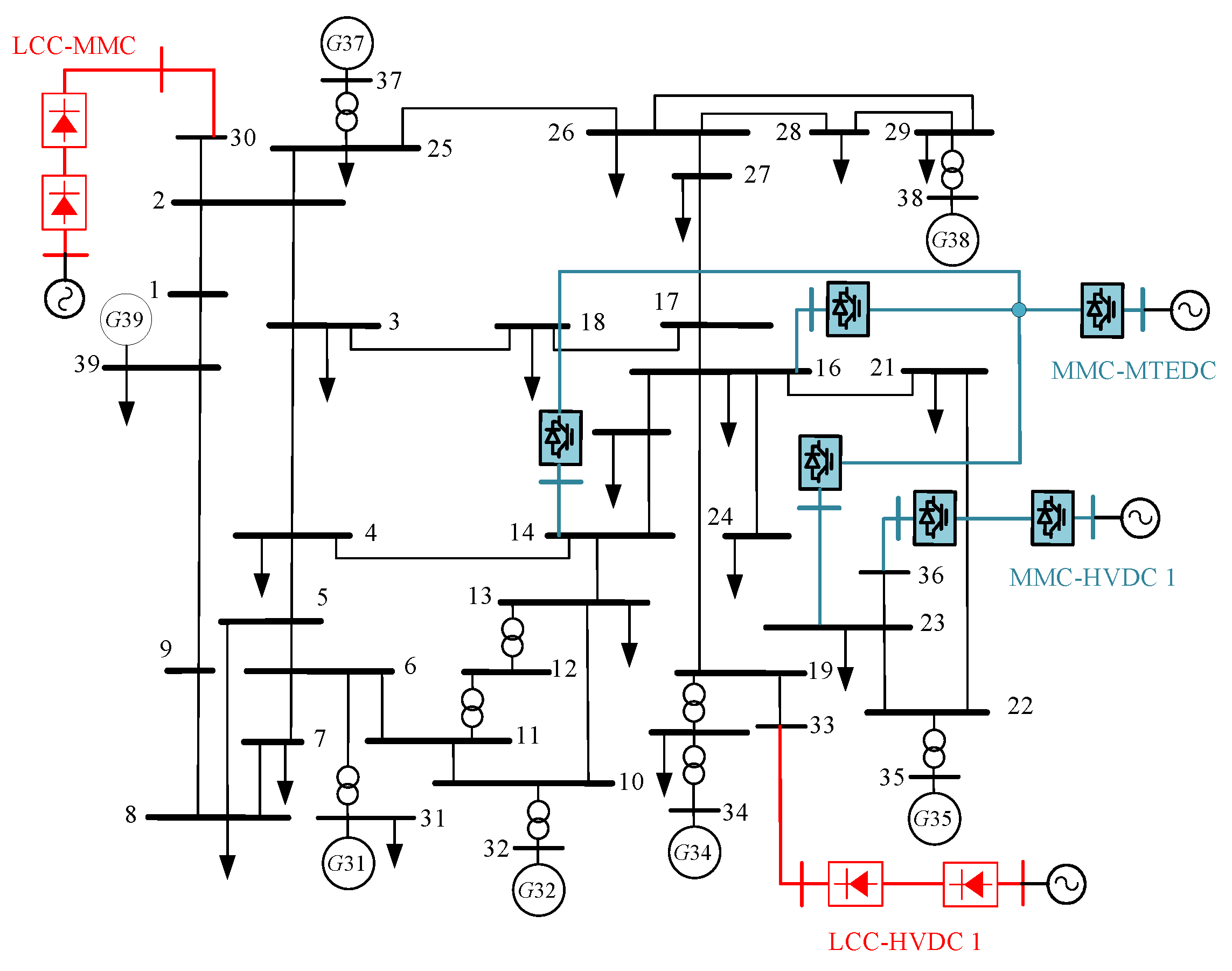
A modified IEEE 39-bus system, shown in Figure 1, is used as the case study to emulate a receiving-end mega-city urban grid that is fed by several LCC-HVDC links and that incorporates a four-terminal MMC-MTEDC system. Relative to the standard 39-bus system, four main modifications are made. First, the generators originally at buses 30 and 33 are replaced by LCC-HVDC landing points, and the generator at bus 36 is replaced by a standalone MMC-HVDC injection point. Second, an MMC converter station is connected to each of internal buses 14, 16, and 23 within the urban load area; these stations are interconnected through a DC star network, and one sending-end port injects external active power into the DC network. Third, the synchronous machines at buses 31, 32, 34, 35, 37, and 38 are retained as constant-PV units, and bus 39 serves as the slack machine (representing the equivalent external main grid). Fourth, the loads are rescaled on the basis of the standard power-flow data and are assigned 24 h normalized daily load curves according to three categories—industrial, residential, and commercial. The overall system scale and settings are listed in

Table 1. Overall scale and settings of the test system.

Item	Scale/Value	Item	Scale/Value
Total AC buses	39	Active load buses	19
Total AC branches	48 (buses 16–17 are three parallel circuits)	Nominal total load	6098.1 MW/1408.9 MVar
Synchronous generators	7 (6 PV + slack machine at bus 39)	24 h peak/valley load	5530 MW (18:00)/3487 MW (03:00)
LCC-HVDC landing points	2 (buses 30 and 33)	Daily load factor	0.631
MMC-MTEDC system	Three terminals (14, 16, and 23) + 1 sending port	Base external received power (scale = 1)	2290 MW
Standalone MMC-HVDC	1 (bus 36)	System/DC base	$S_{\mathrm{b}\mathrm{a}\mathrm{s}\mathrm{e}}$ = 100 MVA; $V_{dc,\mathrm{b}\mathrm{a}\mathrm{s}\mathrm{e}}$ = 400 kV

.

The active-power limits, terminal voltages, and fuel costs of the synchronous generators are listed in

Table 2. Parameters of the synchronous generators.

Bus	Role	${\mathit{P}}_{\mathbf{m}\mathbf{i}\mathbf{n}}$, MW	${\mathit{P}}_{\mathbf{m}\mathbf{a}\mathbf{x}}$, MW	Base Output, MW	Terminal Voltage, pu	Fuel Cost, ($·MWh−1)
31	PV	150	650	520	1.02	18
32	PV	150	725	650	1.02	15
34	PV	150	610	508	1.02	20
35	PV	150	685	560	1.02	17
37	PV	150	660	540	1.02	19
38	PV	200	920	830	1.02	14
39	Slack	0	1100	—	1.03	16

; the total installed capacity of the synchronous machines is 5350 MW (including 1100 MW for the slack machine), and the spinning-reserve coefficient is taken as 5%. The LCC-HVDC infeed parameters are listed in

Table 3. LCC-HVDC infeed parameters.

Landing Bus	Base Infeed Active Power, MW	Reactive-Power Characteristic
30	450	Reactive absorption $\approx k_{q}P\left(1-{\eta }_c\right)$, $k_q=0.5$, compensation factor of 1.05
33	280	As above

; their reactive-power consumption increases as the infeed active power rises and worsens further when the voltage drops, reflecting the “destabilizing” characteristic described in Section 2.2. The parameters of the MMC-MTEDC system and the DC network are listed in

Table 4. MMC-MTEDC system and DC-network parameters.

Converter Station (Bus)	Control Mode	${\mathit{S}}^{\mathbf{m}\mathbf{a}\mathbf{x}}$, MVA	Active-Power Limit, MW	AC-Voltage Set-Point, pu
14	Constant reactive power	1500	1500	—
16	Constant AC voltage	800	800	1.02
23	DC-voltage slack + constant AC voltage	380	Following	1.03
Sending port	External active-power injection	—	$P_{send}=1000$	—

: station 14 is under constant-reactive-power control, station 16 under constant-AC-voltage control, and station 23 serves additionally as the DC-voltage slack station while also under constant-AC-voltage control; the sending-end port injects an external active power $P_{send}=1000$ MW; and the DC network has a star topology centered on the intermediate node $s$, connecting buses 14/16/23 through DC resistances.

The DC network has a star topology; the DC resistances $R_{dc}$ ($send$–14, $send$–16, and $send$–23) are 2.8, 4.1, and 2.5 Ω, respectively; the converter efficiency is $\eta =0.98$; the slack-station DC voltage is 1.01 pu (base of 400 kV); and the number of edges of the inscribed polygon for the capability-curve approximation is $L=16$.

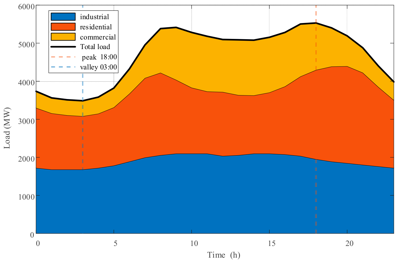
To reflect the time-varying load characteristics of the urban grid, the industrial, residential, and commercial loads are each assigned a 24 h normalized daily load curve (with a peak multiplier of 1.00): the industrial load is high by day and low by night with relatively small fluctuation throughout the day; the residential load exhibits an evening peak, reaching its maximum at 20:00; and the commercial load is high during the daytime, reaching full load over 10:00–15:00. After superposition of the three categories, the system-wide peak load occurs at 18:00 (5530 MW), the valley load occurs at 03:00 (3487 MW), and the daily load factor is 0.631.

The base external received power (scale = 1) consists of the sending-port active power, the two LCC infeeds, and the standalone MMC-HVDC:

$$P_{rec}^{\left(0\right)}=P_{send}+\sum P_{lcc}+P_{indep}=1000+\left(450+280\right)+560=2290\hspace{0.25em}\mathrm{M}\mathrm{W}$$

(42)

To avoid ambiguity, the maximum receiving capability is defined and measured as follows. The external received power P_rec is the total active power imported into the receiving-end AC grid, namely, the net active power delivered through the MMC-MTEDC sending port plus the two LCC-HVDC infeeds plus the standalone MMC-HVDC; the DC-network losses are deducted (they are borne by the DC slack station), so that P_rec is the power actually injected at the receiving-end AC buses rather than the power dispatched at the sending side. The maximum receiving capability is then the largest P_rec for which a feasible unit-commitment solution exists that simultaneously satisfies the static-voltage-stability constraint τ_min ≥ τ_th, the converter-capability limits, the line-loading limits and the voltage limits, all verified on the full non-linear AC/DC power flow, as described in Section 4.3. Regarding the load model, the case study uses a constant-power representation for all loads (i.e., the ZIP coefficient a_P = 1, with the constant-current and constant-impedance shares set to zero), which is the most demanding case for static voltage stability.

The case study raises the external received power synchronously by a factor, and two evaluation modes are distinguished. The peak-load single-snapshot method scans the received power only on the peak-load snapshot, until the unit commitment first becomes infeasible. The 24-period time-series method lets the imported power follow the normalized load shape $w\left(t\right)$ (with $w=1$ at the peak); a given level of received power is “feasible” if and only if a feasible unit commitment is obtained for all 24 snapshots and is therefore more stringent.

5.2. Receiving Capability and Stability Margin Under the Peak-Load Single Snapshot

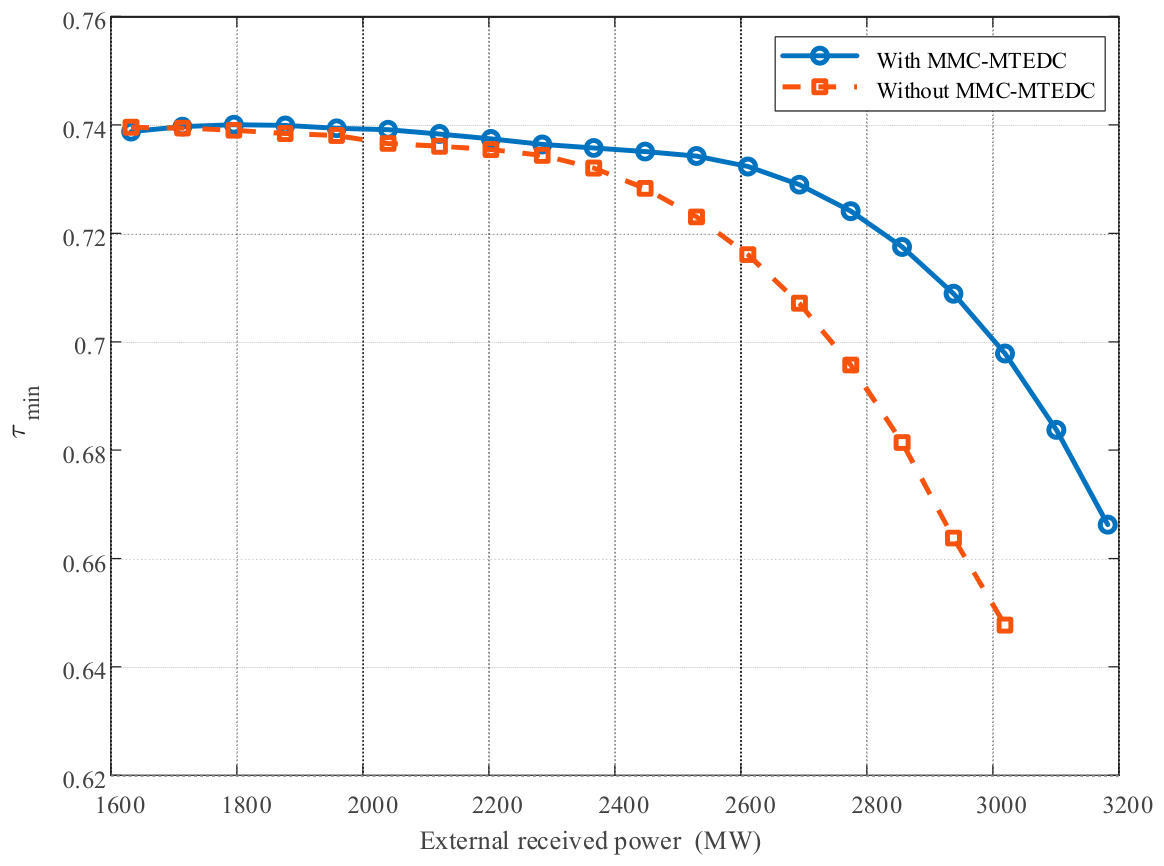
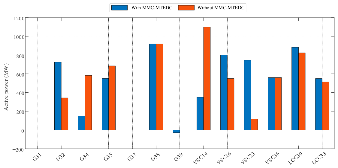
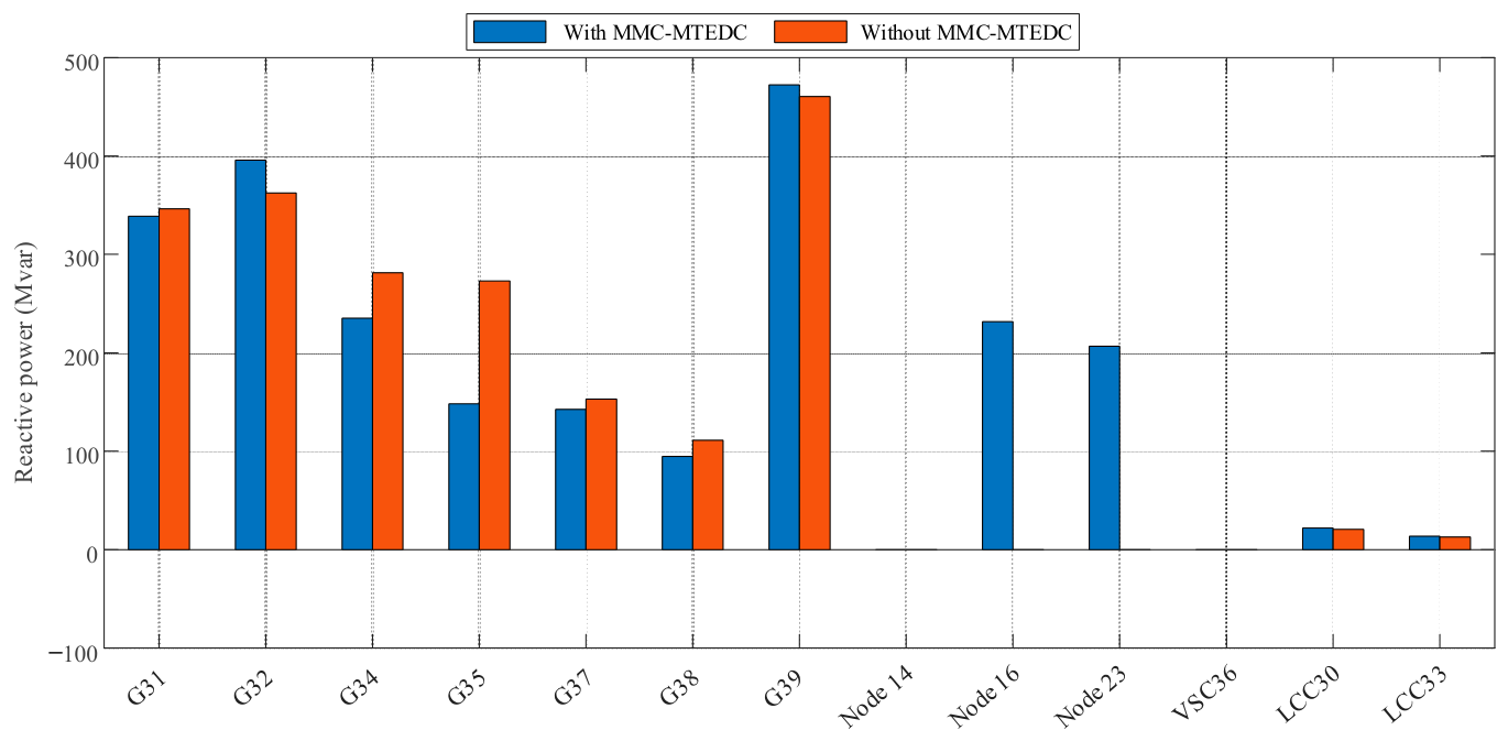
On the peak-load snapshot (18:00, 5530 MW), the optimal-dispatch model is solved by the CCG iteration of Section 4.3, and the minimum singular value ${\tau }_{\mathrm{m}\mathrm{i}\mathrm{n}}$ of the augmented extended power-flow Jacobian is recorded point by point. The resulting comparison curves of ${\tau }_{\mathrm{m}\mathrm{i}\mathrm{n}}$ versus the external received power are shown in Figure 2, and the comparisons of the active/reactive-power outputs of the synchronous machines and DC converter stations are shown in Figure 3 and Figure 4. The solver settings and computational performance is shown in

Table 5. Solver settings and computational performance.

Item	Value/Setting
Solver	MATLAB intlinprog
Programming environment	MATLAB R2024a
Hardware	12-core, 64-bit Windows workstation; CPU: 12th Gen Intel(R) Core(TM) i7-12700K, 32.0GB RAM
Convergence criterion (Step 5)	Objective change < 1.0 cost unit and non-linear feasibility within 1 × 10−3
CCG iterations to converge	1–6 (median 2; iteration cap 12)
Peak-load single-snapshot assessment time	≈1.9 s
24-period whole-day assessment time	≈18.5 s

.

In Figure 2, the abscissa is the external received power, and the ordinate is ${\tau }_{\mathrm{m}\mathrm{i}\mathrm{n}}$ (0.62–0.76), with the horizontal dashed line indicating the stability threshold ${\tau }_{th}=0.62$. The blue solid line is the MMC-MTEDC case, and the orange dashed line is the without-MMC comparison case. In both cases, ${\tau }_{\mathrm{m}\mathrm{i}\mathrm{n}}$ decreases monotonically as the received power increases; however, the with-MMC curve lies entirely above the without-MMC curve, and the gap between the two widens as the received power grows. The mechanism is consistent with the sensitivity analysis in Section 3.2: a constant-AC-voltage-controlled MMC converts the connected bus from a “voltage-free, collapse-prone” bus into a voltage-supported PV-type bus, raising the static-voltage-stability margin at the same level of received power. In the without-MMC case, the unit commitment first becomes infeasible at about 3030 MW (the curve terminates there, with ${\tau }_{\mathrm{m}\mathrm{i}\mathrm{n}}\approx 0.648$), whereas the with-MMC case can extend to about 3220 MW, which intuitively demonstrates that the dynamic support of the MMC-MTEDC system not only raises the margin but also expands the feasible receiving range.

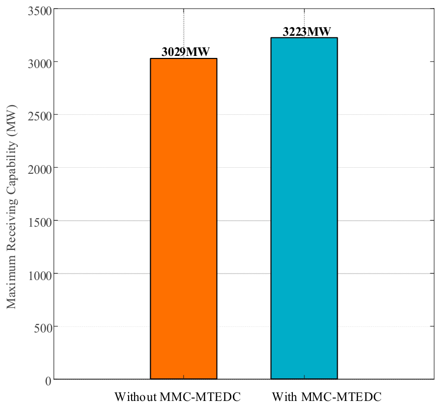
The maximum receiving capability of the peak-load snapshot in the two cases is further obtained, as shown in Figure 5: 3029 MW without MMC and 3223 MW with MMC-MTEDC (corresponding to scale ≈ 1.408). That is, the four-terminal MMC-MTEDC system raises the maximum receiving capability of the peak-load snapshot by 194 MW, a relative increase of about 6.4%. This is the core quantitative result of the case study, and it quantitatively verifies the effectiveness of the MMC-MTEDC system in enhancing the receiving capability of the receiving-end urban grid.

It is worth noting that when the received power reaches its limit, the binding bottleneck of the system is that ${\tau }_{\mathrm{m}\mathrm{i}\mathrm{n}}$ touches the vicinity of its threshold and that the converter station reaches its capability-curve limit and is forced to degrade from constant-AC-voltage control to constant-reactive-power control—rather than a line thermal limit or a bus-voltage violation. This is consistent with the paper’s basic argument that “the maximum receiving capability of a receiving-end urban grid is constrained by the static-voltage-stability margin.”

5.3. Decomposition of the Contribution of the MMC-MTEDC System

To clarify the source of the improvement and to establish its academic value, the effect of the MMC-MTEDC system is decomposed into four mechanisms—① active-power redistribution through the DC network, ② reactive-power and voltage support, ③ the effect of switching the AC-voltage-controlled (V-control) bus, and ④ the addition of an extra receiving source—through four controlled sub-cases evaluated on the peak-load cross-section and summarized in

Table 6. Decomposition of the contribution of the MMC-MTEDC system on the peak-load cross-section.

Case	Description	Max. Receiving Capability (MW)	Critical τmin at the Maximum Feasible Receiving Level
F	Full MMC-MTEDC system (active + reactive support + capability limit)	3223	0.624
(a)	Active injection only (voltage control removed)	2906	0.629
(b)	Redistribution and support only (Psend = 0)	1466	0.655
(c)	Ideal case (capability-curve constraint removed)	3358	0.621
(d)	Equal-rating reactive compensation (= without MMC-MTEDC system)	3029	0.648

. In sub-case (a), all MMC stations are set to constant-reactive-power control with fixed reactive power, so the converter performs active-power injection and DC redistribution but provides no voltage support, isolating ① + ④ from ② + ③. In sub-case (b), the external active import is removed (P_send = 0), while voltage control is retained, so that only internal redistribution and voltage support remain, isolating ① + ② + ③ from ④; the receiving base for this sub-case is 1290 MW, since the sending-port import is removed. In sub-case (c), the converter-capability constraint is relaxed so that no stations are ever forced to degrade from constant-AC-voltage to constant-reactive-power control, removing the margin-decline mechanism ③ and revealing the upper bound of the benefit. In sub-case (d), the MMC-MTEDC system is replaced by a reactive-power compensator of the same reactive rating at the same buses (the “without-MMC-MTEDC” baseline), isolating the marginal benefit of the controllable converter over an equal-rating static reactive device.

Table 6 shows that the full MMC-MTEDC system raises the maximum receiving capability to 3223 MW, compared with 3029 MW for the equal-rating reactive compensation (d); the controllable converter therefore provides about 194 MW (6.4%) of additional capability beyond an equal-rating static device, which is the marginal value of mechanisms ①–③ acting together. Removing the voltage support (a) lowers the capability to 2906 MW, confirming that reactive and voltage support ② is a major contributor, whereas relaxing the capability limit (c) raises it to 3358 MW, indicating that the forced V-to-Q degradation ③ is what ultimately caps the benefit. Sub-case (b) isolates pure redistribution and support and shows that even without any external import, the MMC-MTEDC system sustains 1466 MW on a 1290 MW base, so mechanisms ① + ② + ③ are individually beneficial; the remaining gap from the full case is attributable to the extra-source mechanism ④. The decomposition thus attributes the overall improvement primarily to the controllable reactive and voltage support and to the avoidance or postponement of the V-to-Q degradation, with active-power redistribution and the additional receiving source providing complementary contributions. It should be noted that the magnitude of the observed improvement is dependent on the siting and capacity of the MMC converter stations—a converter located at a voltage-weaker bus or endowed with larger capability headroom generally yields a larger margin gain.

5.4. Whole-Day Receiving Capability Considering 24-Period Transmission Cross-Sections

The peak-load single-snapshot method verifies only the single most severe instant and may therefore overestimate the received power that is feasible throughout the day. The 24-period time-series method is therefore adopted: the imported power follows the normalized load shape $w\left(t\right)$ (with $w=1$ at the peak); a transmission cross-section is constructed period by period, and the unit commitment is solved; and a given scale is “feasible” if and only if a feasible unit commitment is obtained for all 24 snapshots of the day. The system-wide 24 h daily load curve (superposed by category), which serves as the import-following factor, is shown in Figure 6, with a peak load of 5530 MW (18:00) and a valley load of 3487 MW (03:00).

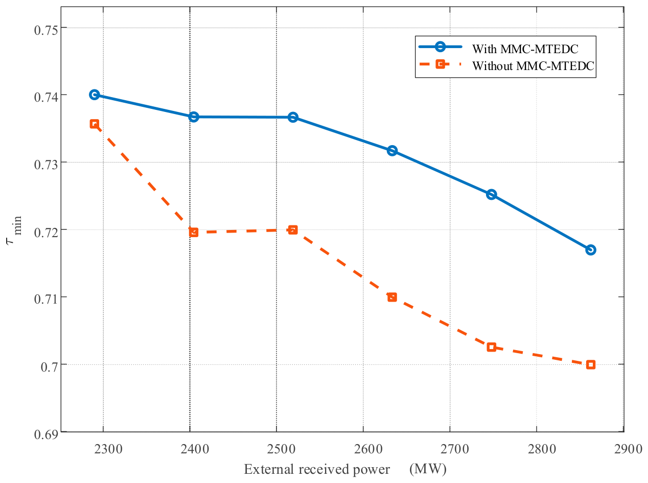
Under the time-series method, the receiving capability is measured by the imported power at the peak-load instant. Figure 7 presents the ${\tau }_{\mathrm{m}\mathrm{i}\mathrm{n}}$ curves versus the imported power for the peak-load cross-section (the most stressed cross-section of the day); the with-MMC curve always lies above the without-MMC curve. The endpoint of the with-MMC case is about 2860 MW, corresponding to a whole-day maximum receiving scale of 1.244. This indicates that among the 24 cross-sections, the peak-load cross-section is the binding cross-section.

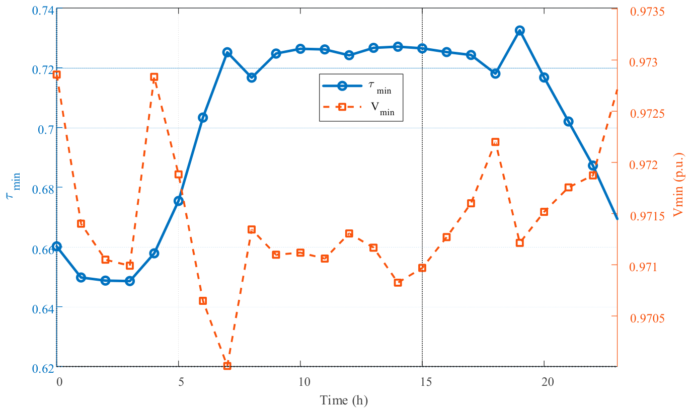
To confirm the time-series feasibility, Figure 8 presents the period-by-period verification of the stability and voltage margins at the whole-day maximum receiving scale (scale = 1.244, with MMC-MTEDC); the left ordinate is ${\tau }_{\mathrm{m}\mathrm{i}\mathrm{n}}$ (blue solid line with circles, 0.62–0.74), and the right ordinate is the minimum bus voltage $V_{\mathrm{m}\mathrm{i}\mathrm{n}}$ (orange dashed line with squares, approximately 0.9705–0.9735), with the horizontal dashed line indicating ${\tau }_{th}=0.62$. As can be seen, ${\tau }_{\mathrm{m}\mathrm{i}\mathrm{n}}$ for all 24 cross-sections of the day exceed the threshold of 0.62 (with the lowest being about 0.648 over 01:00–04:00 and the highest about 0.73 at midday), while $V_{\mathrm{m}\mathrm{i}\mathrm{n}}$ remains above 0.97 throughout. This shows that the true bottleneck of the whole-day received power is the static-voltage-stability margin ${\tau }_{\mathrm{m}\mathrm{i}\mathrm{n}}$ rather than the bus-voltage magnitude, which again corroborates this paper’s argument. It also indicates that the 3223 MW obtained by the peak-load single-snapshot method is an upper limit applicable only to the peak-load snapshot, whereas the feasible peak-instant imported power computed on the whole-day time-series basis is about 2849 MW—a more stringent measure that is of greater engineering reference value.

6. Conclusions

For a receiving-end mega-city urban grid that has LCC-HVDC infeed and incorporates MMC-MTEDC, this paper proposes a method for assessing the maximum receiving capability under the static-voltage-stability constraint and verifies it on a modified IEEE 39-bus system. The main conclusions are as follows:

• The established quasi-steady-state model of the receiving-end urban grid—considering LCC infeed and an MMC-MTEDC system—characterizes, through the DC-network equations, the mutual coupling among the AC active-power injections of the receiving-end converter stations and uniformly represents the three roles of the MMC-MTEDC system, namely, external power import, power-flow redistribution, and voltage support.
• By adopting as the static-voltage-stability index the minimum singular value ${\tau }_{\mathrm{m}\mathrm{i}\mathrm{n}}$ of the augmented extended Jacobian—which incorporates the MMC control equations and the DC power-flow equations—the block upper-triangular structure of this matrix is proved, and the sensitivities of ${\tau }_{\mathrm{m}\mathrm{i}\mathrm{n}}$ to the synchronous-machine outputs and the MMC active/reactive decisions (coupled through the DC network) are derived. The analysis reveals that a constant-AC-voltage-controlled MMC converts a “voltage-free, collapse-prone” bus into a voltage-supported PV-type bus and thereby raises the margin, whereas as the received power increases, a converter station that reaches its capability-curve limit is forced to degrade from constant-AC-voltage control to constant-reactive-power control, and the margin then declines.
• The established unit-commitment optimization model—centered on the ${\tau }_{\mathrm{m}\mathrm{i}\mathrm{n}}$ constraint and accounting for the converter-capability curve (inscribed-polygon approximation), the voltages of critical industrial-load buses, and the line-loading limits—uses column-and-constraint generation (CCG) to iteratively correct the sensitivity-linearization error and uses the feasibility of the unit commitment as the criterion for estimating the maximum receiving capability, thereby incorporating “how much can be received” and “how to operate” within a unified framework.
• The case-study results show that the MMC-MTEDC system raises the maximum receiving capability of the peak-load snapshot from 3029 MW to 3223 MW (a relative increase of about 6.4%); by the more stringent 24-period time-series measure, the whole-day feasible receiving scale is 1.244.

However, three refinements indicated by the modeling assumptions of this study are left for future work: embedding an explicit minimum-extinction-angle constraint for the LCC, so that commutation-failure immunity is enforced rather than assumed; using a CPF for out-of-optimization, post-contingency verification of the proximity to voltage collapse, complementing the singular-value index employed inside the optimization; and replacing the constant-efficiency converter model with a state-dependent loss model (for example, a piecewise-linear loss curve in the converter current) to refine the available reactive-power headroom and the thermal limits. In addition, future work may proceed along the following directions: first, account for N-1 security constraints and the interactions among multiple DC infeeds, extending the assessment method to probabilistic and multi-scenario settings; second, incorporate dynamic-voltage-stability and frequency-security constraints into a unified assessment framework to more closely approximate engineering practice; third, study the optimal siting and sizing of the MMC-MTEDC system so as to maximize the benefit of enhancing the receiving capability of the receiving-end urban grid; and fourth, a rigorous, system-dependent prescription of the stability threshold τ_th and its replacement by a CPF-validated, analytically grounded criterion.

References

1. Shair, J.; Li, H.; Hu, J.; Xie, X. Power system stability issues, classifications and research prospects in the context of high-penetration of renewables and power electronics. Renew. Sustain. Energy Rev. 2021, 145, 111111. [Google Scholar] [CrossRef] [Scilit]
2. Wang, W.; Li, G.; Guo, J. Large-scale renewable energy transmission by HVDC: Challenges and proposals. Engineering 2022, 19, 252–267. [Google Scholar] [CrossRef] [Scilit]
3. Hatziargyriou, N.; Milanović, J.; Rahmann, C.; Ajjarapu, V.; Cañizares, C.; Erlich, I.; Hill, D.; Hiskens, I.; Kamwa, I.; Pail, B.; et al. Definition and classification of power system stability—Revisited and extended. IEEE Trans. Power Syst. 2021, 36, 3271–3281. [Google Scholar] [CrossRef] [Scilit]
4. Kim, Y.-K.; Lee, G.S.; Kim, C.-K.; Moon, S.-I. An improved AC system strength measure for evaluation of power stability and temporary overvoltage in hybrid multi-infeed HVDC systems. IEEE Trans. Power Deliv. 2022, 37, 638–649. [Google Scholar] [CrossRef] [Scilit]
5. Deng, B.; Wen, Y. Admissible HVDC infeed capacity evaluation of receiving-end power grids. Int. J. Electr. Power Energy Syst. 2023, 146, 108760. [Google Scholar] [CrossRef] [Scilit]
6. Wang, H.; Ke, D.; Xu, J.; Liao, S.; Jiang, X.; Si, T.; Pan, X. Determination of HVDC infeed transfer capacity regions for receiving-end grids via multi-objective frequency-secured unit commitment: A hierarchical approach. Int. J. Electr. Power Energy Syst. 2026, 177, 111813. [Google Scholar] [CrossRef] [Scilit]
7. Sun, K.; Xiao, H.; Pan, J.; Liu, Y. VSC-HVDC interties for urban power grid enhancement. IEEE Trans. Power Syst. 2021, 36, 4745–4753. [Google Scholar] [CrossRef] [Scilit]
8. Jiang, X.; Zhou, Y.; Ming, W.; Yang, P.; Wu, J. An overview of soft open points in electricity distribution networks. IEEE Trans. Smart Grid 2022, 13, 1899–1910. [Google Scholar] [CrossRef] [Scilit]
9. Zhai, J.; Dai, X.; Jiang, Y.; Xue, Y.; Hagenmeyer, V.; Jones, C.N.; Zhang, X.P. Distributed optimal power flow for VSC-MTDC meshed AC/DC grids using ALADIN. IEEE Trans. Power Syst. 2022, 37, 4861–4873. [Google Scholar] [CrossRef] [Scilit]
10. Ergun, H.; Dave, J.; Van Hertem, D.; Geth, F. Optimal power flow for AC-DC grids: Formulation, convex relaxation, linear approximation, and implementation. IEEE Trans. Power Syst. 2019, 34, 2980–2990. [Google Scholar] [CrossRef] [Scilit]
11. Ambia, M.N.; Meng, K.; Xiao, W.; Al-Durra, A.; Dong, Z.Y. Adaptive droop control of multi-terminal HVDC network for frequency regulation and power sharing. IEEE Trans. Power Syst. 2021, 36, 566–578. [Google Scholar] [CrossRef] [Scilit]
12. Xiao, J.; Li, F.; Gu, W.; Wang, C.; Zhang, P. Total supply capability and its extended indices for distribution systems: Definition, model calculation and applications. IET Gener. Transm. Distrib. 2011, 5, 869–876. [Google Scholar] [CrossRef] [Scilit]
13. Xiao, J.; Wang, C.; She, B.; Li, F.; Bao, Z.; Zhang, X. Total supply and accommodation capability curves for active distribution networks: Concept and model. Int. J. Electr. Power Energy Syst. 2021, 133, 107279. [Google Scholar] [CrossRef] [Scilit]
14. Wang, X.; Wang, X.; Sheng, H.; Lin, X. A data-driven sparse polynomial chaos expansion method to assess probabilistic total transfer capability for power systems with renewables. IEEE Trans. Power Syst. 2021, 36, 2573–2583. [Google Scholar] [CrossRef] [Scilit]
15. Löf, P.-A.; Smed, T.; Andersson, G.; Hill, D.J. Fast calculation of a voltage stability index. IEEE Trans. Power Syst. 1992, 7, 54–64. [Google Scholar] [CrossRef] [Scilit]
16. Chu, Z.; Teng, F. Voltage stability constrained unit commitment in power systems with high penetration of inverter-based generators. IEEE Trans. Power Syst. 2023, 38, 1572–1582. [Google Scholar] [CrossRef] [Scilit]
17. Guo, J.; Zou, L.; Zhang, N.; Jia, Y.; Pan, X.; Sun, X. Coordinated active and reactive power control of VSC-HVDC for enhancing static voltage stability in AC/DC systems. Energies 2025, 18, 6127. [Google Scholar] [CrossRef] [Scilit]
18. Taghavi, M.; Delkhosh, H.; Parsa Moghaddam, M.; Sheikhi Fini, A. Hosting capacity enhancement of hybrid AC/DC distribution network based on static and dynamic reconfiguration. IET Gener. Transm. Distrib. 2023, 17, 3765–3780. [Google Scholar] [CrossRef] [Scilit]
Figure 1. Architecture of the modified IEEE 39-bus system.
Energies 19 03333 g001
Figure 2. Minimum singular value τ m i n versus external received power.
Energies 19 03333 g002
Figure 3. Comparison of synchronous-machine active/reactive-power outputs.
Energies 19 03333 g003
Figure 4. Comparison of DC converter-station active/reactive-power outputs.
Energies 19 03333 g004
Figure 5. Maximum receiving capability in the two cases.
Energies 19 03333 g005
Figure 6. System-wide 24 h daily load curve.
Energies 19 03333 g006
Figure 7. τ m i n of the peak-load cross-section versus imported power.
Energies 19 03333 g007
Figure 8. Period-by-period τ m i n and minimum bus voltage V m i n at the whole-day maximum receiving scale.
Energies 19 03333 g008