A Multi-Objective Short-Term Complementary Scheduling Model for Hydro-Wind-Solar Systems Considering Conditional Value-at-Risk

Abstract

The large-scale integration of wind and solar power has significantly intensified peak-shaving pressure and operational risk in provincial power grids. Effectively leveraging the flexible regulation capability of hydropower to mitigate the uncertainty of wind and solar output is a promising approach to enhancing grid security and stability. To simultaneously improve the peak-shaving performance and risk resilience of hydro-wind-solar systems for a provincial power grid, this paper proposes a multi-objective short-term scheduling model that jointly minimizes the peak value of net load and the Conditional Value-at-Risk (CVaR) of flexibility shortage. Specifically, the residual peak load is used to quantify the system’s peak-shaving burden, while the average CVaR of upward/downward ramping deficits across all time periods characterizes the tail risk associated with insufficient flexibility. Historical wind and solar forecast error data are employed to generate representative uncertainty scenarios via Gaussian mixture model, and the Rockafellar–Uryasev formulation is adopted to accurately embed CVaR into a mixed-integer linear programming (MILP) framework. Furthermore, the normalized normal constraint (NNC) method is introduced to compute a well-distributed Pareto front. Numerical simulations based on a real-world hydro-wind-solar system in a provincial grid in Southwest China demonstrate that the proposed model can significantly reduce the peak load while effectively mitigating flexibility shortfall risk. The resulting Pareto front clearly reveals the trade-off between peak-shaving effectiveness and risk control, providing a scientific basis for day-ahead generation scheduling and coordinated dispatch of flexible resources.

1. Introduction

As China continues to implement its national strategy of peaking carbon dioxide emissions before 2030 and achieving carbon neutrality before 2060, the penetration of renewable energy sources such as wind and solar power in the electricity system is steadily increasing. On 25 April 2025, China’s installed capacity of wind and solar power reached exceeding the installed capacity of thermal power for the first time [1]. By the end of 2025, China’s installed wind power capacity reached 640 GW, and installed solar power capacity stood at 1.2 billion kW. The combined capacity of wind and solar power was 1.84 billion kW, accounting for 47% of the country’s total installed power capacity, and has become the most important power source in China [2]. However, the high variability and uncertainty of wind and solar output significantly exacerbate the peak-valley difference and ramp-up rates of net load, potentially leading to insufficient balancing capacity, curtailment of wind and solar power presents significant challenges for power system dispatching and operation [3,4]. Hydropower, with its rapid response capability, large-scale energy storage potential, and excellent load-following and frequency regulation performance, has become an important source of flexibility for integrating high penetration of renewable energy [5]. Currently, it has emerged as a critical research focus operation.

The integration of variable renewable energy (VRE) sources fundamentally alters power system operation patterns [6]. Unlike conventional dispatchable generation, VRE output exhibits high intermittency and limited predictability, necessitating enhanced system flexibility to maintain supply–demand balance [7]. Extensive research on hydro-wind-solar coordinated scheduling has been mainly conducted from two perspectives: operational mechanism analysis and optimization modeling [8,9,10]. In terms of scheduling time scales, existing studies span multiple levels, including medium to long-term planning, day-ahead scheduling, and intra-day real-time dispatch [11,12,13,14,15]. Medium- to long-term operation primarily focuses on reservoir operation strategies and the renewable sources configuration, playing a crucial role in long-term generation planning and hydropower utilization [16,17], making short-term scheduling more sensitive to real-time fluctuations and extreme events [18,19]. As the penetration of renewable energy increases, short-term scheduling becomes more and more important in hybrid hydro-wind-solar complement operation [20,21].

To address the short-term scheduling of hybrid hydro-wind-solar systems, existing studies mainly adopt methods such as deterministic optimization, stochastic optimization, and robust optimization approaches [22,23,24,25,26]. Deterministic models rely on forecast values and are unable to cope with extreme scenarios. Stochastic optimization typically optimizes expected performance but often pays insufficient attention to low-probability and high-impact scenarios. Although robust optimization enhances system security margins, it often results in overly conservative scheduling outcomes. With high renewable penetration, short-term hydro-wind-solar scheduling must simultaneously balance multiple, often competing objectives—including operational economy, renewable energy curtailment minimization, hydropower operational safety, and overall system stability. Consequently, single-objective models fail to capture the real-world operational requirements. Therefore, short-term hydro-wind-solar scheduling inherently involves multi-objective decision-making and requires comprehensive trade-offs under a multi-objective framework [27]. Recent efforts have begun to explore multi-objective short-term scheduling for hydro-wind-solar systems. For instance, Xu et al. [28] proposed a multi-objective coordinated scheduling method for hybrid hydro-wind-solar-storage systems, and analyzed the synergies and trade-offs among objectives under representative scenarios. Zhou et al. [29] developed a multi-objective scheduling model for a grid-connected hydro-wind-solar-battery system under extreme weather scenarios to minimize load shedding and carbon dioxide emission. Wang et al. [30] proposed a short-term optimal scheduling model of hybrid hydro-wind-solar-thermal and pumped hydro storage, with objectives of minimizing thermal power operation cost, maximizing renewable energy power generation. However, the aforementioned studies mainly focus on operational costs and power generation, without addressing the operational risks under extreme scenarios, thereby leaving a critical gap in ensuring system resilience under high uncertainty.

Within a multi-objective short-term scheduling framework, quantitatively characterizing the extreme operational risks induced by renewable energy uncertainty is crucial to enhancing both the security and practicality of scheduling solutions. Conditional Value-at-Risk (CVaR) provides an effective measure of the expected loss under adverse tail-end scenarios. With its favorable mathematical properties, CVaR has been widely applied in risk-aware decision-making for electricity markets and power systems with high renewable penetration. For example, Ju et al. [31] developed a virtual power plant scheduling model integrating hydro, wind, solar, and energy storage, incorporating CVaR into the objective function and constraints to quantify the uncertainty risk of renewable output. Jia et al. [32] proposed a risk-averse optimization model for a hybrid wind-solar-storage system, employing CVaR to capture the uncertainty in renewable generation. Similarly, Nieta et al. [33] utilized CVaR to evaluate bidding strategies in electricity markets, specifically to study risk hedging of bidding strategies for the hybrid hydro-wind system. However, research that systematically integrates CVaR into multi-objective short-term hydro-wind-solar complementary scheduling models to depict the trade-off between peak-shaving performance and operational risk remains relatively limited.

Based on the above analysis, this paper proposes a multi-objective coordinated optimization framework that balances peak shaving effects and flexibility insufficient risks. The main contributions are as follows:

(1) A bi-objective short-term hydro-wind-solar scheduling model is proposed that explicitly captures the trade-off between peak-shaving performance and flexibility shortage tail risk, which has been largely overlooked in existing studies that focus on operational cost or generation maximization.

(2) CVaR is adopted to quantify flexibility shortage tail risk, and the Rockafellar–Uryasev method is employed to cast CVaR into a MILP framework, ensuring both computational tractability of the risk measure and solvability of the overall model.

(3) The NNC method is adopted (not proposed as novel) to address the specific deficiency of uneven Pareto front distribution caused by objectives with vastly different scales and curvatures.

The remainder of this paper is organized as follows. Section 2 presents the mathematical formulation of the proposed model. Section 3 details the solution methodology. Section 4 presents a case study based on a real-world hybrid hydro-wind-solar system in southwest China. Finally, Section 5 concludes the paper with key findings and implications.

2. Mathematical Model

2.1. Wind and Solar Power Scenario Generation

2.1.1. Description of Wind and Solar Output Uncertainty

Wind and solar power generation are highly sensitive to weather conditions, exhibiting significant variability and uncertainty that hinder high-accuracy forecasting. In provincial power system scheduling, due to the aggregation effect resulting from geographic diversity, when multiple wind farms and solar power stations located in different geographic areas are aggregated, the overall output’s random fluctuations are mitigated, thereby effectively reducing forecasting errors. To leverage this aggregation benefit while simplifying model complexity, this study aggregates all wind farms within the province into a single virtual wind farm and all solar plants into a single virtual solar plant.

$$P_t^W={\displaystyle \sum _{i=1}^{N^W}}{P}_{i,t}^W$$

(1)

$$P_t^S={\displaystyle \sum _{i=1}^{N^S}}{P}_{i,t}^S$$

(2)

where $P_{i,t}^W$ and $P_{i,t}^S$ denote the power output of wind plant i and solar plant i at time period t, respectively; $N^W$ and $N^S$ represent the total number of wind farms and solar power plants; and $P_t^W$ and $P_t^S$ are the aggregated outputs of the virtual wind plant and virtual solar plant at period t, respectively.

A reasonable description of wind and solar output uncertainty is important for effective hydro-wind-solar complementary scheduling. Existing studies have shown that the forecast errors of wind and solar power do not follow a specific parametric distribution [34]. Gaussian mixture model (GMM), as a non-parametric density estimation approach, offer greater flexibility compared to traditional parametric methods. By representing the underlying distribution as a weighted sum of multiple Gaussian components, GMM can theoretically approximate any continuous probability distribution. Therefore, this paper employs GMM to describe the uncertainty in wind and solar output. Let be a random variable. The probability density function of a single Gaussian distribution is given by:

$$f\left(x\mathrm{丨}\mu ,\sigma \right)={\displaystyle \frac{1}{\sqrt{2{\sigma }^2\pi }}}{e}^{-{\displaystyle \frac{{\left(x-\mu \right)}^2}{2{\sigma }^2}}}$$

(3)

The GMM is essentially a linear combination of multiple Gaussian distributions, and its expression can be described as:

$$p\left(x\right)={\displaystyle \sum _{n=1}^G}{\omega }_n\mathsf{\phi }\left(x\mathrm{丨}{\mu }_n,{\sigma }_n\right)$$

(4)

where $p\left(x\right)$ denotes the pdf of $x$; ${\omega }_n$ is the weight of n-th component, and ${\displaystyle {\sum }_{n=1}^G}{\omega }_n=1$. The parameters ${\omega }_n$, ${\mu }_n$, and ${\sigma }_n$ can be estimated using the maximum likelihood estimation method.

To objectively determine the optimal number of Gaussian components G without artificial subjective selection, the Bayesian Information Criterion (BIC) is adopted in this paper to balance the data fitting accuracy and model complexity of GMM. For a given G, the BIC is defined as:

$$\mathrm{BIC}(G)=-2{\sum }_{i=1}^N\mathrm{l}\mathrm{n}\rho (x_i)+M(G)\mathrm{l}\mathrm{n}N$$

(5)

where N is the number of observed samples, $\rho \left(x_i\right)$ is the likelihood of the i-th sample under the fitted GMM, and $M\left(G\right)$ denotes the total number of independent parameters of the GMM. The optimal G is obtained by:

$$G^{*} =\arg {\mathrm{m}\mathrm{i}\mathrm{n}}_{G\in \{\mathrm{1,2},\dots ,G_{max}\}}\mathrm{B}\mathrm{I}\mathrm{C}(G)$$

(6)

The first term in the BIC penalizes poor model fit, while the second term penalizes excessive model complexity. As G increases, the likelihood term decreases monotonically, but the penalty term grows linearly. The BIC automatically balances these two competing objectives, and the value of G that minimizes BIC(G) is selected as the optimal number of components.

Using historical data as input samples, the prediction errors for wind and solar power at time t are defined as:

$${\epsilon }_t^W(i)=P_t^{W,a}(i){-P}_t^{W,f}(i)$$

(7)

$${\epsilon }_t^S(i)=P_t^{S,a}{(i)-P}_t^{S,f}(i)$$

(8)

where ${\epsilon }_t^W$ and ${\epsilon }_t^S$ denote the forecast errors of wind and solar power generation at time t, respectively; $P_t^{W,a}$ and $P_t^{W,f}$ represent the actual and forecasted wind power outputs at time t; and $P_t^{S,a}$ and $P_t^{S,f}$ denote the actual and forecasted solar power outputs at time t.

Using GMM, the forecast error distributions for wind and solar at each time period are obtained:

$${\widehat{f}}_t^W\left(\mathsf{\epsilon }\right)={\displaystyle \frac{1}{Nh}}{\sum }_i\kappa \left({\displaystyle \frac{\mathsf{\epsilon }-{\epsilon }_t^W\left(i\right)}{h}}\right)$$

(9)

$${\widehat{f}}_t^S\left(\epsilon \right)={\displaystyle \frac{1}{Nh}}{\sum }_i\kappa \left({\displaystyle \frac{\mathsf{\epsilon }-{\mathsf{\epsilon }}_t^S\left(i\right)}{h}}\right)$$

(10)

where ${\widehat{f}}_t^W\left(\mathsf{\epsilon }\right)$ and ${\widehat{f}}_t^S\left(\epsilon \right)$ are the estimated pdfs of wind and solar forecast errors at time t, respectively; N is the number of historical error samples; $h$ is the bandwidth; and $\kappa (·)$ is the kernel function.

2.1.2. Wind and Solar Output Scenario Generation

A set of K error scenarios is generated by sampling from the wind and solar forecast error distributions:

$${\epsilon }_t^{W,\left(k\right)}~{\widehat{f}}_t^W\left(\epsilon \right)$$

(11)

$${\epsilon }_t^{S,\left(k\right)}~{\widehat{f}}_t^S\left(\epsilon \right)$$

(12)

Then, the wind and solar output scenarios are obtained as:

$$P_{t,k}^W=P_t^{W,f}+{\epsilon }_t^{W,\left(k\right)}$$

(13)

$$P_{t,k}^S=P_t^{S,f}+{\epsilon }_t^{S,\left(k\right)}$$

(14)

where ${\epsilon }_t^{W,\left(k\right)}$ and ${\epsilon }_t^{S,\left(k\right)}$ denote the wind and solar power forecast errors at time t under the k-th scenario, respectively; $P_{t,k}^W$ and $P_{t,k}^S$ are the wind and solar outputs at time $t$ for the $k$-th scenario.

In this study, K = 1000 scenarios are generated via Monte Carlo sampling from the fitted GMM distributions for each time period independently. Each scenario is assigned equal probability $p_k=1/\mathrm{K}$. To ensure physical feasibility, any sampled wind or solar output that falls below zero is truncated to 0, and any value exceeding the installed capacity is capped at the nominal capacity.

2.2. Measurement of Power Grid Flexibility

2.2.1. Flexibility Demand

The system’s flexibility demand is defined as the deviation between actual wind and solar power output and their forecasted values. By summing up the upward and downward flexibility demands for wind and solar energy, respectively, the overall flexibility demands for renewable energy can be expressed as follows:

$$R_{t,k}^{\uparrow }=\max \left(0,-\left(P_{t,k}^W-P_t^{W,f}\right)-\left(P_{t,k}^S-P_t^{S,f}\right)\right)$$

(15)

$$R_{t,k}^{\downarrow }=\max \left(0,\left(P_{t,k}^W-P_t^{W,f}\right)+\left(P_{t,k}^S-P_t^{S,f}\right)\right)$$

(16)

where $R_{t,k}^{\uparrow }$ and $R_{t,k}^{\downarrow }$ denote the upward and downward flexibility demands at time t under scenario k, respectively.

2.2.2. Flexibility Supply Capability

Hydropower provides flexibility for wind and solar power. The flexibility supply capability of hydropower is calculated as follows:

$$F_t^{\uparrow }={\displaystyle \sum _{m=1}^M}\min \left({\overline{P}}_m^H-P_{m,t}^H,\Delta {\overline{P}}_m^H\right)$$

(17)

$$F_t^{\downarrow }={\displaystyle \sum _{m=1}^M}\min \left(P_{m,t}^H-{\underset{\_}{P}}_m^H, \Delta {\overline{P}}_m^H\right)$$

(18)

where $F_t^{\uparrow }$ and $F_t^{\downarrow }$ represent the upward and downward flexibility supply capabilities of hydropower at time $t$, respectively; ${\overline{P}}_m^H$, ${\underset{¯}{P}}_m^H$, $P_{m,t}^H$ and $\mathsf{\Delta }{\overline{P}}_m^H$ represent the maximum output, minimum output, scheduling output and maximum ramping capability of hydropower station $m$, respectively.

It should be noted that Equations (17) and (18) provide an approximate upper-bound estimate of the instantaneous flexibility supply based on capacity headroom and ramping limits. In practice, the actual flexibility available from the hydro system is further constrained by water balance dynamics, reservoir level bounds, turbine discharge limits, cascade travel time, tailwater effects, and head-dependent generation characteristics, all of which are captured by the full set of hydropower constraints (Equations (29)–(42)) in the scheduling model. Therefore, while the flexibility shortage risk metric may slightly overestimate the available flexibility margin, the actual dispatch decisions produced by the optimization model remain physically feasible under all operational constraints.

2.3. Flexibility Shortage Risk Analysis

Based on the above analysis, when the flexibility demand exceeds the flexibility supply capability, a flexibility shortage occurs, which can be expressed as:

$$U_{t,k}^{\uparrow }=\max ({R_{t,k}^{\uparrow }-F}_t^{\uparrow },0)$$

(19)

$$U_{t,k}^{\downarrow }=\max (R_{t,k}^{\downarrow }-F_t^{\downarrow },0)$$

(20)

where $U_{t,k}^{\uparrow }$ and $U_{t,k}^{\downarrow }$ represent the upward and downward flexibility shortages at time $t$ for scenario $k$. The total flexibility shortage for scenario $k$ at time period $t$ is defined as:

$$U_{t,k}=U_{t,k}^{\uparrow }+U_{t,k}^{\downarrow }$$

(21)

In the context of high penetration of wind and solar power, the power system faces significant output uncertainty, and scientific methods are required to assess and address the resulting flexibility shortage risks. Current mainstream methods include Value at Risk (VaR) and Conditional Value at Risk (CVaR). VaR only provides the loss threshold at a certain confidence level, making it simple to calculate but neglecting tail extreme losses [35]. In contrast, CVaR is a consistent risk measure that satisfies fine mathematical properties such as subadditivity and convexity. CVaR focuses on tail risks and can effectively characterize the average loss under the most adverse scenarios, achieving a good balance between economic efficiency and security [36]. Therefore, this paper adopts CVaR to assess flexibility shortage risk. Assuming the loss function is:

$$L_{t,k}=a^{\uparrow }{U}_{t,k}^{\uparrow }+a^{\downarrow }{U}_{t,k}^{\downarrow }$$

(22)

where $L_{t,k}$ represents the flexibility shortage loss at time $t$ for scenario $k$, and $a^{\uparrow }$ and $a^{\downarrow }$ are the coefficients for upward and downward flexibility shortage losses, respectively.

$${\mathcal{L}}_t=\left\{L_{t,1},L_{t,2},\dots ,L_{t,K}\right\}$$

(23)

Given a confidence level of $\alpha$, the empirical VaR for period $t$ is:

$${VaR}_{\alpha ,t}=L_{\left(⌈\alpha K⌉\right)}$$

(24)

Correspondingly, the empirical CVaR for that time period is:

$${CVaR}_{\alpha ,t}={\displaystyle \frac{1}{\left(1-\alpha \right)K}}\sum _{k:L\left(t,K\right)\ge {VaR}_{\alpha ,t}} L_{t,k}$$

(25)

2.4. Overall Mathematical Model

2.4.1. Objective Functions

The large-scale integration of wind and solar power into provincial power grid presents significant challenges for short-term power system scheduling, mainly appeared in the following aspects: (1) The peak value of the grid has expanded dramatically. The solar power output concentrated during the midday significantly reduces net load during noon hours, while the high wind power output at night overlaps with the low-load valley, resulting in a net load showing “deep valley” and “steep peaks” which significantly increases the difficulty of peak shaving [37]. (2) Under extreme weather conditions, wind and solar forecast errors can far exceed typical ranges; without sufficient system flexibility, this may lead to grid security issues. In short-term hydro-wind-solar coordinated scheduling, the peak-shaving objective directly affects operational efficiency and economic performance, whereas the flexibility shortage risk is related to system security and resilience. Therefore, this study builds a bi-objective optimization scheduling model that addresses both peak shaving and grid flexibility shortage risk.

(1) Peak-Shaving Objective

The peak value of net load is adopted as the peak-shaving metric because it directly reflects the operating range that thermal generating units must accommodate. A large net load peak value usually means a large peak-valley difference and forces thermal units into frequent deep cycling and start-stop operations, which increases fuel consumption, equipment wear, and overall operating costs. Reducing this difference alleviates the peak-shaving burden on thermal generators, lowers spinning reserve requirements, and enhances system reliability. Although alternative metrics such as ramping cost or load-following cost have been used in the literature, minimize the peak value of residual load remains the most widely adopted indicator in Chinese provincial grid dispatching practice, as it directly determines the minimum operating range for thermal units and is straightforward to interpret and implement in day-ahead scheduling.

The first objective is to minimize the peak value of the residual load. This can be expressed as:

$$f_1=\min \begin{array}{c}{\displaystyle \sum _{k=1}^{\mathrm{K}}}{p}_k\left(\underset{1\le t\le T}{\max }{C}_{k,t}\right)\end{array}$$

(26)

$$C_{t,k}=L_t-{\displaystyle \sum _{m=1}^M}{P}_{m,t}^H-P_{t,k}^W-P_{t,k}^{PV}$$

(27)

where $L_t$ is the original load at time period $t$; $p_k$ is the probability of scenario k; $C_{t,k}$ is the residual load for scenario $k$ at time $t$. This objective aims to minimizing the peak value of residual load and smoothing the residual load and facilitating efficient and stable operation of other power sources such as coal-fired units.

(2) Flexibility shortage risk objective

The second objective minimizes the grid’s flexibility shortage risk, using CVaR as the risk measure. The objective function can be expressed as:

$$f_2=\min \left({\displaystyle \frac{1}{T}}{\displaystyle \sum _{t=1}^T}{\mathrm{C}\mathrm{V}\mathrm{a}\mathrm{R}}_{\alpha ,t}\right)$$

(28)

Since ${\mathrm{C}\mathrm{V}\mathrm{a}\mathrm{R}}_{\alpha ,t}$ considers actual scenarios, this objective represents the average risk of flexibility shortage when the hydropower plant is executed under the actual wind and solar output scenarios.

2.4.2. Constraints

Hydropower Constraints

The hydropower system is modeled as a cascade of M reservoirs with hydraulic coupling. The following constraints collectively ensure physically feasible operation: water balance constraints enforce mass conservation in each reservoir, accounting for natural inflow, turbine discharge, spillage, and upstream releases with travel time delay; reservoir water level bounds reflect flood control limits and dead storage requirements; turbine flow and total outflow constraints represent mechanical and environmental flow restrictions; the net head calculation captures the difference between the average forebay level and the tailwater level minus head losses; and the power output function relates generation to the net head and turbine flow through station-specific performance curves. These constraints together capture the key physical characteristics of cascade hydropower operation, including hydraulic coupling between upstream and downstream stations, head-dependent generation efficiency, and operational safety limits.

(1) Water balance constraints

$$V_{m,t+1}=V_{m,t}+\left(Q_{m,t}^{in}-Q_{m,t}^{power}-Q_{m,t}^{loss}\right)\Delta t$$

(29)

$$Q_{m,t}^{in}=Q_{m,t}^{mid}+{\sum }_{i=1}^{{\mathsf{\Omega }}_m}\left(Q_{i,t-{\tau }_{i,m}}^{power}+Q_{i,t-{\tau }_{i,m}}^{loss}\right)$$

(30)

where $V_{m,t}$ is the reservoir storage of m at time period $t$; $Q_{m,t}^{in}$, $Q_{m,t}^{power}$, $Q_{mt}^{loss}$ and $Q_{mt}^{mid}$ denote the inflow, turbine flow, spillage flow, and increment flow during period $t$, respectively; ${\mathsf{\Omega }}_m$ is the set of immediate upstream plants of plant $m$; ${\tau }_{i,m}$ represents the water travel time from upstream plant $i$ to plant $m$; and $\mathsf{\Delta }t$ is the time period length.

(2) Reservoir water level bounds

$${\underset{¯}{Z}}_{m,t}\le Z_{m,t}\le {\overline{Z}}_{m,t}$$

(31)

where ${\overline{Z}}_{m,t}$ and ${\underset{¯}{Z}}_{m,t}$ are the upper and lower limits of the reservoir forebay water level of plant $m$ at time $t$, and $Z_{m,t}$ is the forebay water level of reservoir $m$ at time $t$.

(3) Initial and final water level constraints

$$Z_{m,0}=Z_m^{begin}$$

(32)

$$Z_{m,T}=Z_m^{end}$$

(33)

where $Z_{m,0}$ and $Z_m^{begin}$ denote the initial water level and the given initial water level of station $m$; $Z_{m,T}$ and $Z_m^{end}$ are the final water level and the target final water level at station $m$ at the end of the scheduling period.

(4) Turbine flow constraints

$${\underset{¯}{Q}}_{m,t}^{power}\le Q_{m,t}^{power}\le {\overline{Q}}_{m,t}^{power}$$

(34)

where ${\overline{Q}}_{m,t}^{power}$ and ${\underset{¯}{Q}}_{m,t}^{power}$ represent the upper and lower limits of the turbine flow of station $m$ at time period $t$.

(5) Outflow constraints

$${\underset{¯}{Q}}_{m,t}^{out}\le Q_{m,t}^{out}\le {\overline{Q}}_{m,t}^{out}$$

(35)

$$Q_{m,t}^{out}=Q_{m,t}^{power}+Q_{m,t}^{loss}$$

(36)

where $Q_{m,t}^{out}$ is total discharge of station $m$ at time period $t$; ${\overline{Q}}_{m,t}^{out}$ and ${\underset{¯}{Q}}_{m,t}^{out}$ represent the upper and lower limits of the total outflow.

(6) Hydropower output constraints

$${\underset{\_}{P}}_{m,t}^H\le P_{m,t}^H\le {\overline{P}}_{m,t}^H$$

(37)

where ${\overline{P}}_{m,t}^H$ and ${\underset{\_}{P}}_{m,t}^H$ represent the upper and lower limits of the output at station $m$ at time $t$.

(7) Output ramping constraint

$$\left|P_{m,t+1}^H-P_{m,t}^H\right|\le \Delta {\overline{P}}_m^H$$

(38)

where $\Delta {\overline{P}}_m^H$ is the maximum allowable ramping capacity between consecutive periods for plant $m$.

(8) Net head constraints

$$H_{m,t}={\displaystyle \frac{Z_{m,t-1}+Z_{m,t}}{2}}-Z_{m,t}^{tail}-H_{m,t}^{loss}$$

(39)

where $H_{m,t}$ is the net head of station $m$ at time $t$, $Z_{m,t}^{tail}$ and $H_{m,t}^{loss}$ is the tailwater level and head loss of station $m$ at time $t$.

(9) Water level—storage relationship

$$Z_{m,t}=f_{zv}\left(V_{m,t}\right)$$

(40)

where $f_{zv}(\cdot )$ represents the function for water level and storage capacity relationship.

(10) Tailwater level—discharge relationship

$$Z_{m,t}^{tail}=f_{zq}\left(Q_{m,t}^{out}\right)$$

(41)

where $f_{zq}(\cdot )$ represents the function for tailwater level and discharge flow relationship.

(11) Hydropower output performance function

$$P_{m,t}^H=f_{NQH,m}\left(H_{m,t},Q_{m,t}^{power}\right)$$

(42)

where $f_{NQH,m}(\cdot )$ is the output function of the station m, which is related to the water head and the power generation flow.

System Reserve Constraints

$${\displaystyle \sum _{m=1}^M}\left({\overline{P}}_m^H-P_{m,t}^H\right)\ge \sigma L_t$$

(43)

$${\displaystyle \sum _{m=1}^M}\left(P_{m,t}^H{-\underset{\_}{P}}_m^H\right)\ge \sigma L_t$$

(44)

The above constraints represent the system’s positive and negative reserve constraints, which are generally considered to be a certain percentage of the system load (this paper uses $\sigma$).

3. Model Solution

3.1. Linearization of Objective Functions and Constraints

3.1.1. Linearization of Objective Functions

(1) Linearization of objective function 1

The first objective, which minimizes the peak value of the residual load, can be linearized by introducing auxiliary variables as follows:

$$f_1=\min \begin{array}{c}{\displaystyle \sum _{k=1}^{\mathrm{K}}}{p}_k\left(R_{u,k}\right)\end{array}$$

(45)

Subject to:

$$R_{u,k}\ge C_{t,k};t\in \{\mathrm{1,2}\dots T\}$$

(46)

where $R_{u,k}$ and $R_{d,k}$ are auxiliary variables representing the upper and lower bound of the residual load across all time periods, respectively.

(2) Linearization of objective function 2

To facilitate optimization and integration into the scheduling framework, the CVaR is reformulated using the Rockafellar-Uryasev approach. For a single time period, CVaR at a confidence level can be expressed as:

$${\mathrm{C}\mathrm{V}\mathrm{a}\mathrm{R}}_{\alpha }\left(L_t\right)={\eta }_t+{\displaystyle \frac{1}{1-\alpha }}{\displaystyle \sum _{k=1}^K}{p}_k{z}_{t,s}$$

(47)

$$\left\{\begin{array}{c}{z}_{t,k}\ge L\left(t,k\right)-{\eta }_t\\ z_{t,k}\ge 0\end{array}\right., k\in \{\mathrm{1,2}\dots ,K\}$$

(48)

where ${\eta }_t$ and $z_{t,k}$ are auxiliary variables; ${\eta }_t$ represents ${\mathrm{V}\mathrm{a}\mathrm{R}}_{\alpha }\left(L_t\right)$, i.e., the $\alpha$-quantile of the loss distribution at time t; $z_{t,k}\ge L\left(t,k\right)-{\eta }_t$ and $z_{t,k}\ge 0$ capture the excess loss in scenario beyond the VaR threshold.

Then objective function 2 is transformed into the following linear form:

$$f_2=\min {\displaystyle \frac{1}{T}}{\displaystyle \sum _{t=1}^T}\left({\eta }_t+{\displaystyle \frac{1}{1-\alpha }}{\displaystyle \sum _{k=1}^K}{p}_k{z}_{t,k}\right)$$

(49)

3.1.2. Linearization of Constraints

The flexibility demand and supply expressions can be reformulated as linear constraints.

$$R_{t,k}^{\uparrow }\ge -\left(P_{t,k}^W-P_t^{W,f}\right)-\left(P_{t,k}^S-P_t^{S,f}\right)$$

(50)

$$R_{t,k}^{\downarrow }\ge {(P}_{t,k}^W-P_t^{W,f})+(P_{t,k}^S-P_t^{S,f})$$

(51)

$$R_{t,k}^{\uparrow }\ge 0, R_{t,k}^{\downarrow }\le 0$$

(52)

Specifically, the upward and downward flexibility shortages are modeled as:

$$U_{t,k}^{\uparrow }\ge F_t^{\uparrow }-R_{t,k}^{\uparrow }$$

(53)

$$U_{t,k}^{\downarrow }\ge F_t^{\downarrow }-R_{t,k}^{\downarrow }$$

(54)

$$U_{t,k}^{\uparrow }\ge 0, U_{t,k}^{\downarrow }\ge 0$$

(55)

For nonlinear relationships inherent in hydropower modeling, such as the water level-storage curve and the power output function, there are mature linearization techniques in the literature. Following the approach adopted in [21], this study employs piecewise linear approximations to accurately represent these nonlinear characteristics while preserving model linearity and computational tractability.

3.2. Multi-Objective Solution Method

The proposed model is a typical multi-objective optimization problem. Commonly used multi-objective optimization methods include the weighted-sum method [38], intelligent evolutionary algorithms [39], and the ε-constraint method [40] et al. The weighted-sum method relies heavily on weight selection; intelligent evolutionary algorithms can generate diverse solutions in a single run but usually provide only approximate solutions. The ε-constraint method transforms a multi-objective problem into a single-objective optimization problem by treating one objective as the primary objective and converting the remaining objectives into constraints. By adjusting the ε value, a series of Pareto-optimal solutions can be obtained, which not only satisfy peak-shaving requirements but also quantify flexibility risks under different peak-shaving levels, thereby providing a rigorous decision-making reference for multi-energy complementary scheduling. Therefore, the ε-constraint method is adopted in this study to solve the proposed model.

The ε-constraint method is sensitive to the selection of ε values, and the distribution of solutions depends on the density of ε sampling. Conventional uniform ε settings may result in an uneven distribution of the Pareto front, leading to solution clustering in non-convex or nonlinear regions. The Normalized Normal Constraint (NNC) method constructs originally proposed by Messac et al. [41], constructs subproblems along uniformly distributed normal directions in the normalized objective space and is insensitive to the magnitude of the original objective functions. As a result, it can generate high-quality and evenly distributed Pareto fronts. Accordingly, this paper adopts the NNC-ε approach to solve the multi-objective model. The detailed solution procedure is as follows.

Step 1: Determination of anchor points.

According to the defined peak-shaving objective and risk-minimization objective, the model is solved separately to obtain the anchor points:

(1) Minimize $f_1$ alone to obtain anchor point $A=(f_1^A,f_2^A)$.

(2) Minimize $f_2$ alone to obtain anchor point $B=(f_1^B,f_2^B)$.

Step 2: Construction of the normalized objective space.

The normalized objective functions are defined as:

$${\overline{f}}_1\left(\mathit{x}\right)={\displaystyle \frac{f_1\left(\mathbf{x}\right)-f_1^A}{f_1^B-f_1^A}}$$

(56)

$${\overline{f}}_2\left(\mathit{x}\right)={\displaystyle \frac{f_2\left(\mathbf{x}\right)-f_2^B}{f_2^A-f_2^B}}$$

(57)

After normalization, the objective values are mapped into the interval [0, 1]. The normalized anchor points $\overline{A}$ and $\overline{B}$ are (0, 1) and (1, 0), respectively. The vector pointing from $\overline{A}$ to $\overline{B}$ is given by $\mathbf{n}=(1, -1)$, and the line segment connecting these two anchor points is referred to as the utopia line.

Step 3: Generation of uniformly distributed normal vectors.

Uniformly distributed points are generated along the utopia line. Assuming that the utopia line is divided into $J$ segments, the step size is defined as:

$$\mathit{\delta }=\left({\displaystyle \frac{1}{J-1}},-{\displaystyle \frac{1}{J-1}}\right)$$

(58)

Accordingly, the uniformly distributed points on the utopia line are given by:

$${\mathit{x}}_j=\overline{A}+j·\mathit{\delta },j\in \left\{\mathrm{1,2},\dots ,J-1\right\}$$

(59)

Step 4: Construction of NNC subproblems.

For each point on the utopia line, the following NNC subproblem is formulated:

$$\min {\overline{f}}_2\left(\mathit{x}\right)$$

(60)

$$\mathrm{s}.\mathrm{t}. \left\{\begin{array}{c}\mathit{n}{\left(\mathit{x}-{\mathit{x}}_j\right)}^T\le 0,\\ \mathrm{other} \mathrm{constraints} \mathrm{of} \mathrm{the} \mathrm{original} \mathrm{problem}\end{array}\right.$$

(61)

By solving the subproblems corresponding to each point on the utopia line sequentially, a Pareto front with uniform distribution can be obtained.

4. Case Study

4.1. Background Description

A province in southwestern China is endowed with abundant hydropower resources, and hydropower has served as the dominant source of electricity generation in the region for a long time. To meet the rapidly growing demand for electricity and fulfill low-carbon transformation requirements, the province has vigorously developed wind and solar power. However, the inherent variability and uncertainty introduced by wind and solar power have significant impacts on grid operation. This leads to a mismatch between wind power output and load demand, making grid peak shaving difficult.

The province’s hydropower stations with good regulatory capacity are mainly concentrated in the LC basin, which contains two large-scale reservoirs with yearly or multi-year regulation capacity, serving as the province’s main peak-shaving and frequency regulation resources. This paper focuses on the mid- and lower-reach cascade hydropower stations in the LC basin. Main characteristics of hydropower stations are summarized in

Table 1. Main parameters of the cascade hydropower stations.

Station Name	Installed Capacity (MW)	Regulation Capability	Reservoir Storage (×108 m3)
A	900	Daily	3.2
B	4200	Multi-year	149
C	1670	Seasonal	9.2
D	1350	Seasonal	9.4
E	5850	Multi-year	237
F	1750	Seasonal	11.4

. Additionally, the province’s wind and solar power are aggregated into a virtual wind power station and a virtual solar power station, respectively. Then, a short-term multi-objective hydro-wind-solar coordinated scheduling model is formulated with a 15 min time resolution over a 24 h dispatch horizon. Based on the province’s historical forecast and actual output data over the past five years, the error distribution for each period is calculated using the GMM, and $K=1000$ wind and solar power output scenarios are generated for case study simulation and model evaluation.

Considering the seasonal differences in hydrological inflows between flood and dry periods, as well as the seasonal variability of wind and solar power generation, a typical day in the dry season and a typical day in the flood season are selected for case studies. This enables a comprehensive evaluation of the effectiveness of the proposed model under diverse hydrological and meteorological conditions.

4.2. Single-Objective Comparative Analysis

(1) Typical dry season day

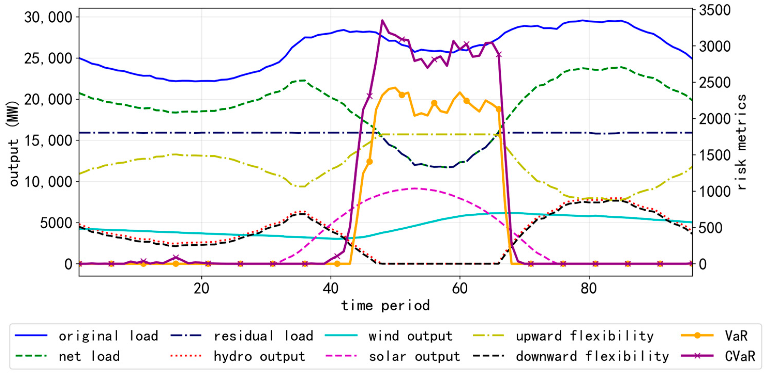
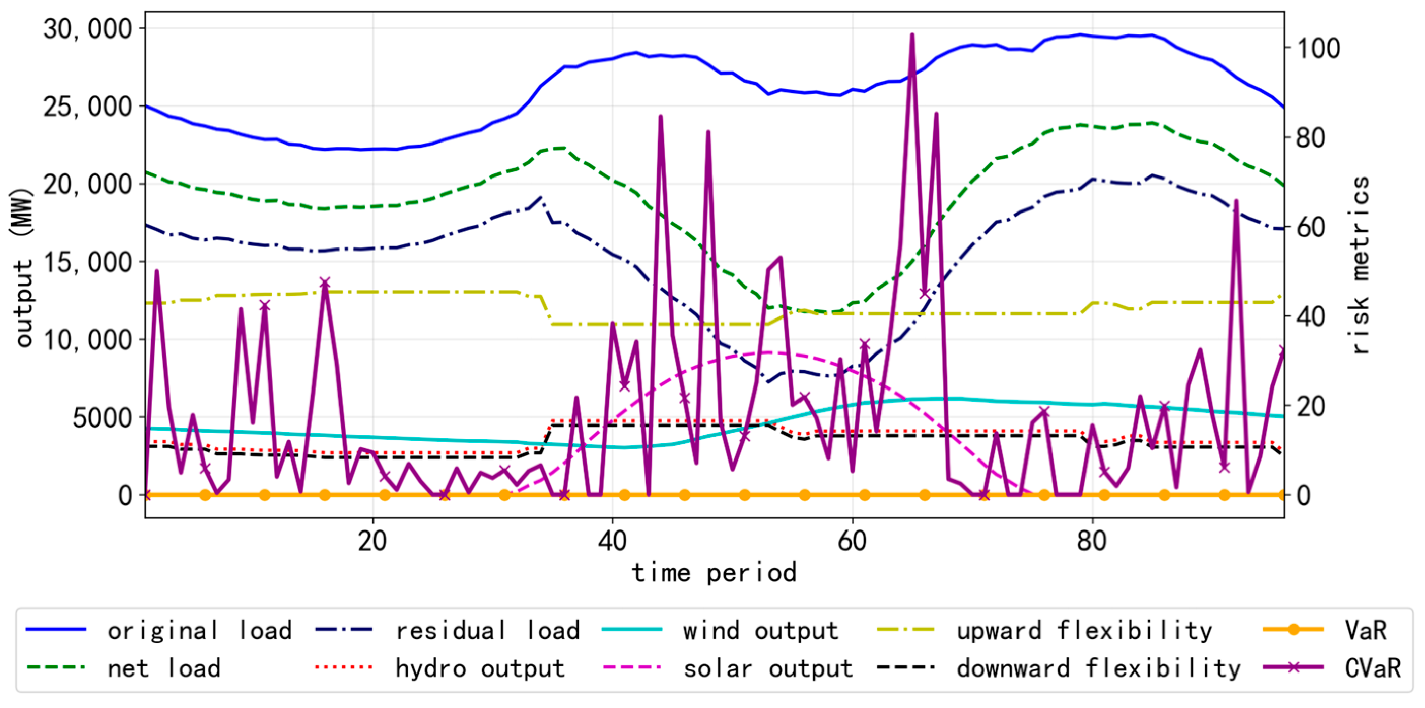
Figure 1 and Figure 2 and

Table 2. Peak-shaving performance under different objectives in the typical dry season day.

Item	Avg (MW)	Max (MW)	Min (MW)	Peak-Valley Difference (MW)	Std. (MW)	Load Rate (%)
Original load	26,115.4	29,575.4	22,168.8	7406.6	2430.6	88.3
Net load	19,036.3	23,889.0	11,710.6	12,178.5	3447.2	79.69
Residual load (peak shaving only)	15,374.6	15,928.3	11,710.6	4217.8	1248.4	96.52
Residual load (risk only)	15,372.2	20,528.5	7242.5	13,286.0	3723.0	74.89

and

Table 3. Flexibility shortage risk under different objectives in typical dry season day.

Item	VaR			CVaR
	Max	Min	Avg	Max	Min	Avg
Peak shaving only	2423.39	0	502.43	3350.96	0	707.48
Risk only	0	0	0	102.88	0	17.94

present the operation results for a typical dry-season day under two single-objective optimization schemes: (i) considering peak-shaving demand only, and (ii) minimizing only the risk of insufficient system flexibility.

As shown in Figure 1 and Table 2 and Table 3, when peak shaving is taken as the objective, hydropower generation is mainly concentrated during load peak periods, while output is reduced during other periods so as to maximize the system’s peak-shaving capability. Under this strategy, the residual load profile remains relatively smooth throughout most of the periods, which is beneficial to the secure and economical operation of thermal power units. However, to accommodate midday solar generation while satisfying peak-shaving requirements, hydropower output is suppressed to a low level during midday hours. Consequently, once the actual wind or solar output exceeds the forecast during these periods, hydropower lacks further downward regulation capability to compensate the power deviation, resulting in a risk of downward flexibility shortage around midday. Moreover, a comparison between the CVaR and VaR curves reveals that CVaR is consistently greater than or equal to VaR, with the discrepancy being particularly evident during midday periods. At several time periods, VaR equals zero while CVaR remains positive. This divergence arises from their fundamental difference in their risk-measurement mechanisms: VaR merely identifies the loss threshold at a given confidence level and ignores tail events beyond that threshold, whereas CVaR explicitly captures tail risks, thereby uncovering hidden operational risks associated with low-probability, high-impact forecast errors.

In contrast, Figure 2 and Table 2 and Table 3 illustrate the operation results when minimizing flexibility shortage risk is the sole objective. In this case, hydropower output is distributed more evenly throughout the day, preserving sufficient regulation capability to accommodate wind and solar power uncertainties and effectively suppressing flexibility shortage risk. However, this strategy leads to a substantial increase in the peak-valley difference in the residual load, thereby significantly aggravating system peak-shaving pressure. It is noteworthy that although VaR is zero in most periods, CVaR remains positive, albeit at a relatively low level. The average CVaR under this strategy is only about 2.5% of that under the peak-shaving-only strategy (shown in Table 3). This can be attributed to limited inflows during the dry season, which limit the overall regulation capability of hydropower. When extreme wind and solar deviations occur, hydropower may still unable to provide sufficient counter-regulation, and CVaR, owing to its sensitivity to tail risks, is able to identify such low-probability but high-consequence operational risks.

In summary, optimizing either peak-shaving performance or flexibility risk alone inevitably exposes the system to non-negligible risks associated with the other objective. This highlights the necessity of jointly considering peak-shaving demand and flexibility shortage risk within a unified scheduling framework to achieve a balanced and coordinated multi-objective solution.

(2) Typical Flood Season Day

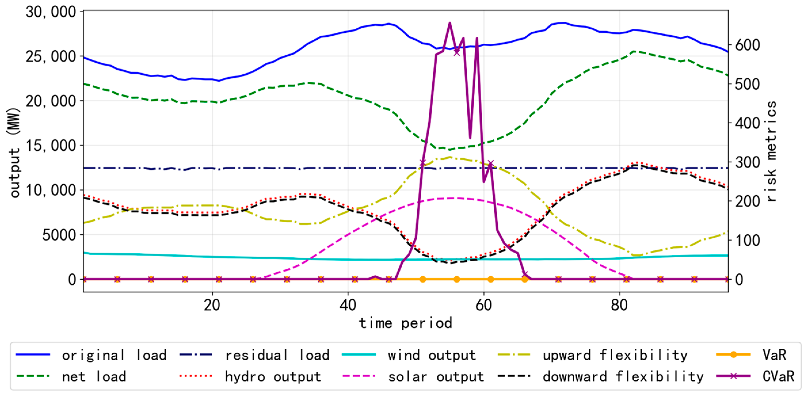
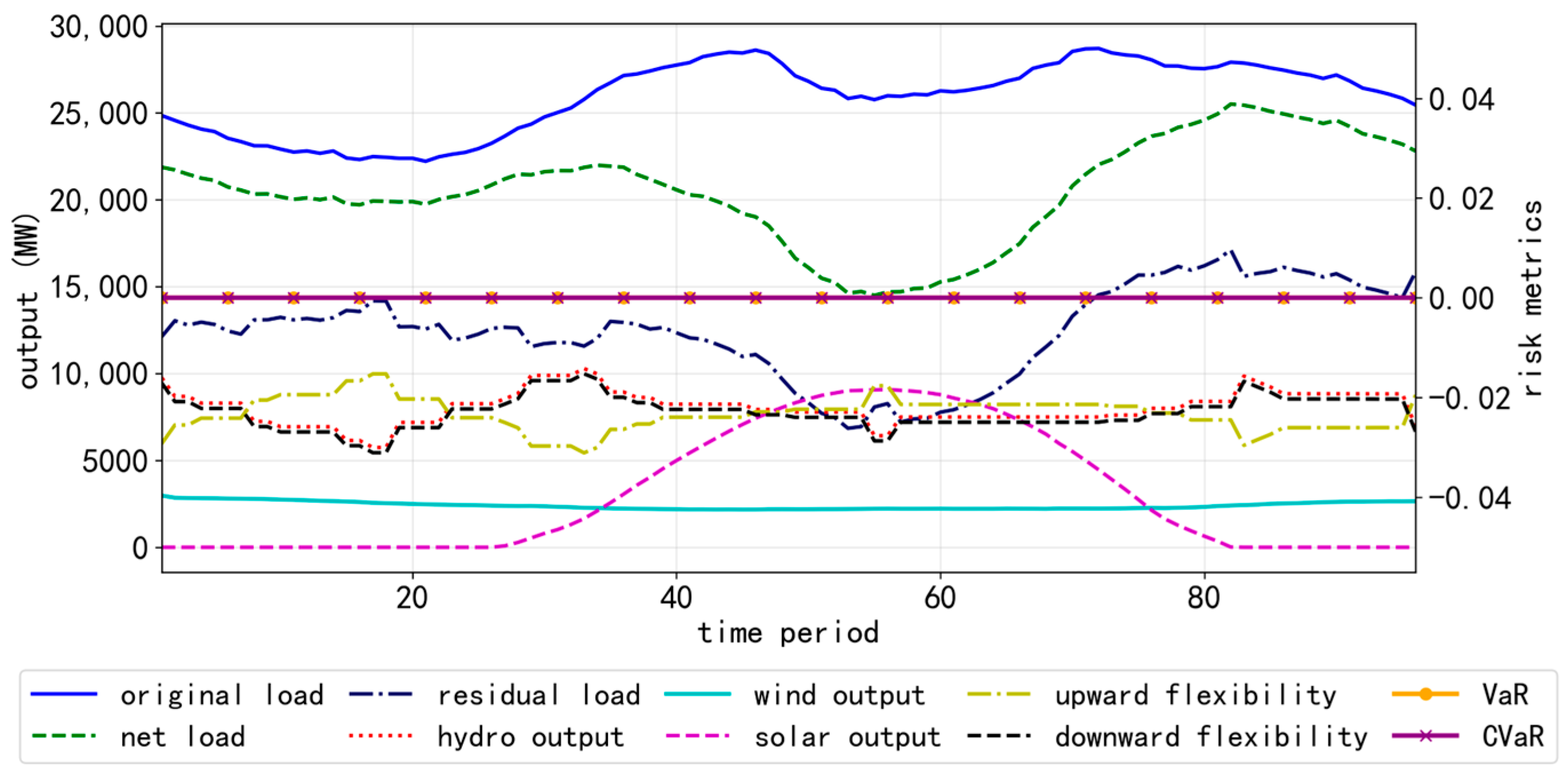
Figure 3 and Figure 4 and

Table 4. Peak-shaving performance under different objectives in the typical flood season day.

Item	Avg (MW)	Max (MW)	Min (MW)	Peak-Valley Difference (MW)	Std. (MW)	Load Rate (%)
Original load	25,914.8	28,711.5	22,217.2	6494.3	2035.5	90.26
Net load	20,485.9	25,510.7	14,496.0	11,014.7	2972.1	80.3
Residual load (peak shaving only)	12,438.7	12,453.8	12,237.8	215.9	43.9	99.88
Residual load (risk only)	12,437.4	17,120.0	6845.9	10,274.0	2615.9	72.66

and

Table 5. Flexibility shortage risk under different objectives in typical flood season day.

Item	VaR			CVaR
	Max	Min	Avg	Max	Min	Avg
Peak shaving only	0	0	0	655.35	0	60.63
Risk only	0	0	0	0	0	0

present the scheduling results for a typical flood season day under two single-objective settings: (i) peak shaving only and (ii) minimization of flexibility shortage risk only.

The results are similar to the dry-season findings. However, during midday periods with high solar power generation, hydropower output has already been reduced to meet peak-shaving requirements, leaving limited downward regulation capability. In contrast, when minimizing flexibility shortage risk is the only objective, hydropower maintains a relatively uniform intraday output, reserving sufficient regulation margins to accommodate wind-solar uncertainty and effectively reducing flexibility risk. Similar to the dry season, this strategy enlarges the peak-valley difference in the residual load, significantly raising peak-shaving pressure within the system.

Notably, compared with the dry-season case, the flexibility shortage risk under the peak-shaving only strategy is substantially lower in the flood season. This difference can be attributed to two main reasons: (i) Higher inflows in the flood season enhance hydropower generation capacity, after meeting peak-shaving requirements, more flexible reserve capacity remains available compared to the dry season. (ii) Wind power output is generally lower in the flood season, the demand for downward regulation is reduced, thus reducing flexibility shortfall risks. Overall, although the flood season features stronger hydropower generation capability, a single-objective strategy still fails to simultaneously satisfy peak-shaving and flexibility requirements. This further underscores the necessity of multi-objective coordinated optimization.

4.3. Multi-Objective Comparative Analysis

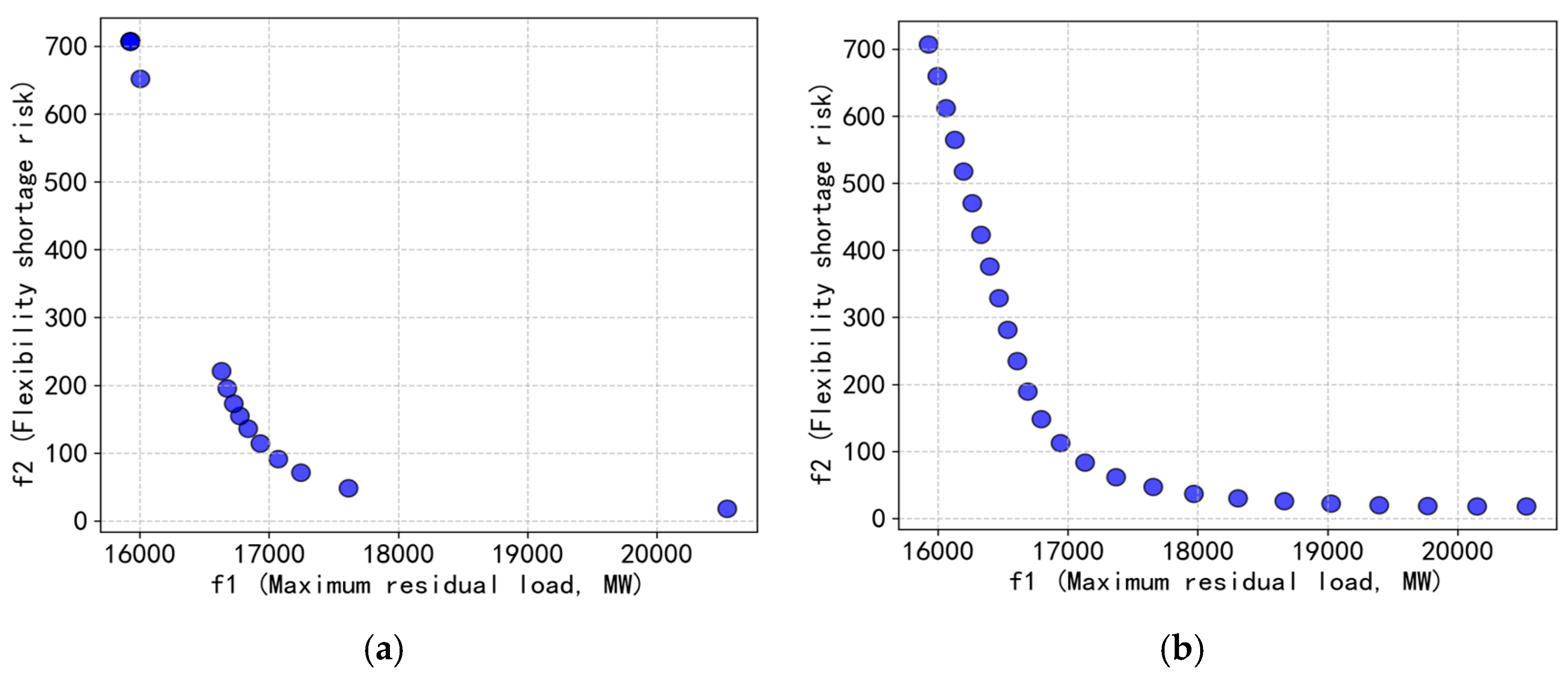
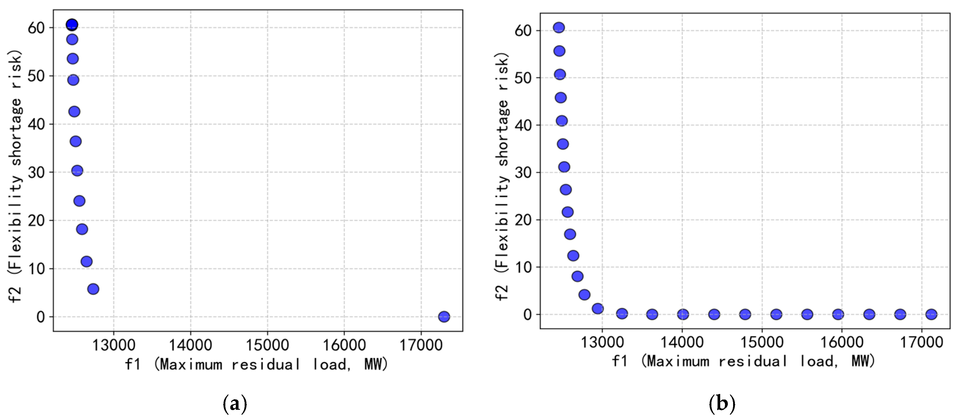
To verify the effectiveness of the NNC method adopted in this study, a comparative analysis is conducted against the conventional weighted method. In the weighted method, two extreme anchor points are first obtained, after which a set of weight combinations is generated with uniform spacing in the weight space, and the corresponding Pareto-optimal solutions are derived by solving weighted single-objective problems. As illustrated in Figure 5 and Figure 6, for conventional weighted method, although the weights are sampled uniformly in the parameter space, the resulting Pareto solutions are distributed highly unevenly in the objective space. A large number of solutions clustered in regions with high curvature of the objective functions, leading to inadequate frontier coverage and limited representativeness of the Pareto front. In contrast, the NNC method performs the search along uniformly distributed normal directions in the normalized objective space, enabling uniform sampling on the objective space. As a result, it produces a Pareto front that is more evenly distributed and provides more comprehensive coverage of the objective space. These results demonstrate that the NNC approach exhibits superior solution diversity and representativeness when dealing with multi-objective optimization problems, and is therefore more suitable for complex system optimization problems such as hydro-wind-solar coordinated scheduling.

4.4. Analysis of Compromise Solutions

The above analysis indicates that optimizing either objective alone leads to a significant deterioration in the other. As Pareto solutions are non-dominated, selecting a satisfactory compromise solution becomes crucial. This study adopts the ideal point method, which selects the Pareto solution with the minimum distance to a virtual ideal point whose components correspond to the best achievable values of each objective on the Pareto front. The method has clear geometric meaning, does not rely on subjective preferences, and objectively evaluates overall performance. In this study, the normalized Euclidean distance is employed as the distance measure, and the procedure is summarized as follows.

(1) Determination of the ideal point: The ideal point ${\mathbf{f}}^{\mathbf{*}} =\left[f_1^{\mathrm{m}\mathrm{i}\mathrm{n}},f_2^{\mathrm{m}\mathrm{i}\mathrm{n}}\right]$ is formed by the best values of each objective within the Pareto solution set:

$${\mathbf{f}}^{\mathbf{*}} =\left[f_1^A,f_2^B\right]$$

(62)

where $f_1^A$ and $f_2^B$ are the individually optimal values of the peak-shaving objective and the flexibility risk objective, respectively, as defined in Section 3.2.

(2) Calculation of the normalized distance: For each Pareto solution $i$, the weighted normalized Euclidean distance to the ideal point is defined as:

$$d_i=\sqrt{{{\omega }_1·\left({\displaystyle \frac{f_{1,i}-f_1^{\mathrm{m}\mathrm{i}\mathrm{n}}}{f_1^{\mathrm{m}\mathrm{a}\mathrm{x}}-f_1^{\mathrm{m}\mathrm{i}\mathrm{n}}}}\right)}^2+{{\omega }_2·\left({\displaystyle \frac{f_{2,i}-f_2^{\mathrm{m}\mathrm{i}\mathrm{n}}}{f_2^{\mathrm{m}\mathrm{a}\mathrm{x}}-f_2^{\mathrm{m}\mathrm{i}\mathrm{n}}}}\right)}^2}$$

(63)

where $f_{1,i}$ and $f_{2,i}$ denote the values of the two objectives for solution $i$; $f_k^{\mathrm{m}\mathrm{a}\mathrm{x}}$ and $f_k^{\mathrm{m}\mathrm{i}\mathrm{n}}$($k=1,2$) are the maximum and minimum values of the $k$-th objective on the Pareto front; and ${\omega }_1$ and ${\omega }_2$ are the corresponding objective weights, ${\omega }_1+{\omega }_2=1$.

(3) Selection of the compromise solution: The compromise solution is identified as the Pareto solution with the minimum distance to the ideal point:

$$i=\arg \underset{i\in \left\{1,\dots ,n\right\}}{\min }{d}_i$$

(64)

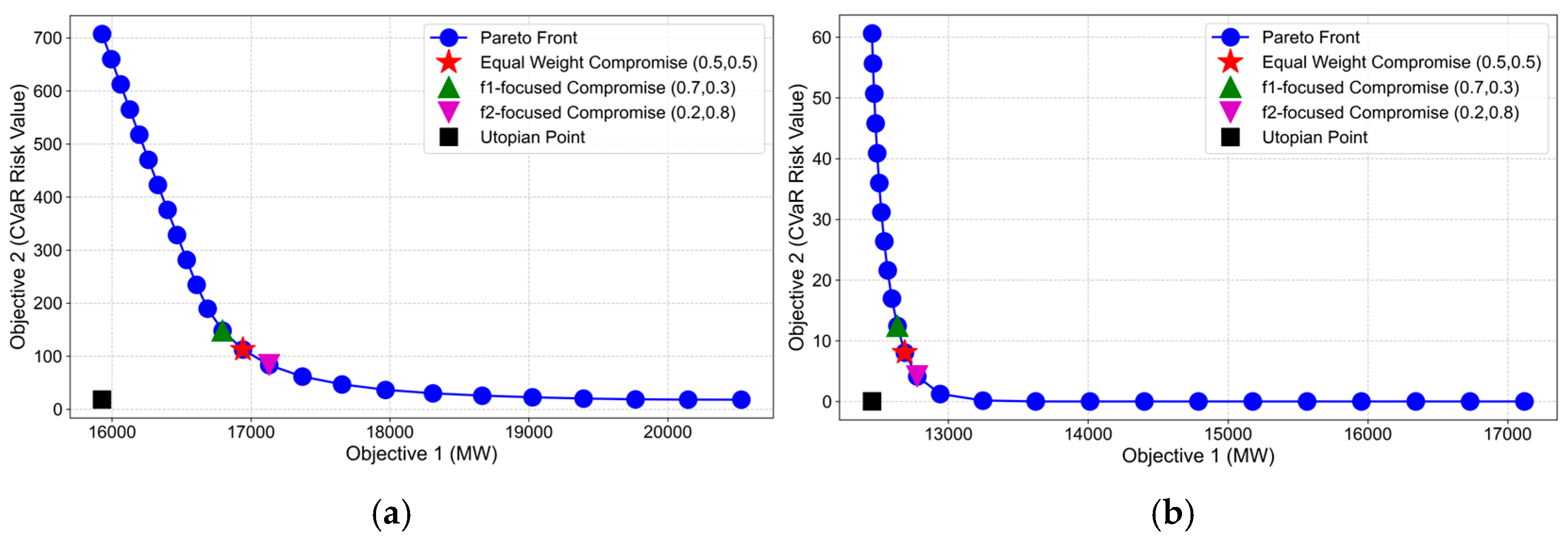
To examine the impact of different preference on scheduling strategies, three weight combinations are considered: $\left({\omega }_1,{\omega }_2)=(\mathrm{0.5,0.5}\right)$, (0.7, 0.3), and (0.3, 0.7), representing balanced preferences, emphasis on peak-shaving performance, and emphasis on flexibility risk control, respectively. Based on these settings, compromise solutions are selected for both typical flood season and dry season typical days. The resulting Pareto fronts and corresponding compromise solutions are illustrated in Figure 7, while the peak-shaving performance and flexibility shortage risk indices under each compromise solution are summarized in

Table 6. Peak-shaving results under different typical weight settings.

Typical Day	Item	Avg (MW)	Max (MW)	Min (MW)	Peak-Valley Difference (MW)	Std. (MW)	Load Rate (%)
Typical dry season day	Residual load (0.5, 0.5)	15,374.6	16,942.5	8892.7	8049.8	2689.9	90.75
	Residual load (0.7, 0.3)	15,373.8	16,796.1	9125.2	7671.0	2552.5	91.54
	Residual load (0.3, 0.7)	15,374.9	17,130.5	8650.9	8479.6	2841.5	89.75
Typical flood season day	Residual load (0.5, 0.5)	12,438.7	12,688.6	10,690.2	1998.4	546.9	98.03
	Residual load (0.7, 0.3)	12,437.5	12,635.2	10,972.7	1662.5	450.5	98.44
	Residual load (0.3, 0.7)	12,439.2	12,776.8	9855.3	2921.5	725.5	97.35

and

Table 7. Flexibility shortage risk under different typical weight settings.

Item	weight Combinations (f1,f2)	VaR			CVaR
		Max	Min	Avg	Max	Min	Avg
Typical dry season day	(0.5, 0.5)	0	0	0	429.75	0	112.49
	(0.7, 0.3)	0	0	0	640.03	0	148.02
	(0.3, 0.7)	0	0	0	333.33	0	83.21
Typical flood season day	(0.5, 0.5)	0	0	0	87.49	0	8.07
	(0.7, 0.3)	0	0	0	119.83	0	12.43
	(0.3, 0.7)	0	0	0	61.54	0	4.16

.

The results show that, in both dry and flood season typical days, the compromise solutions obtained under all three weight settings achieve a satisfactory balance between peak shaving and risk control. Specifically, (1) when greater weight is assigned to Objective 1 (peak shaving), the residual load profile becomes smoother and peak-shaving performance improves, but the system is exposed to a higher risk of downward flexibility shortages; (2) when greater weight is placed on Objective 2 (flexibility risk), the system exhibits stronger capability to accommodate wind and solar output uncertainties, resulting in the lowest risk level, albeit at the expense of peak-shaving performance; and (3) when equal weights are assigned to both objectives, a more balanced trade-off between peak shaving and risk control is achieved. These findings suggest that, in practical operation, weight settings can be flexibly adjusted according to the grid’s prevailing peak-shaving requirements or risk tolerance, thereby enabling adaptive decision-making under multi-objective coordination.

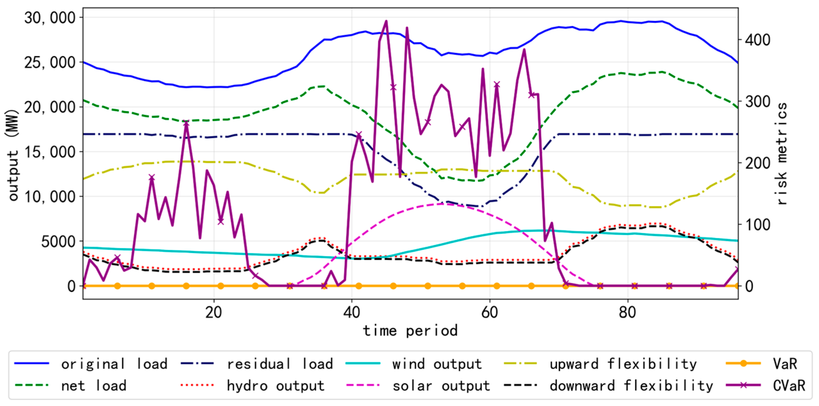
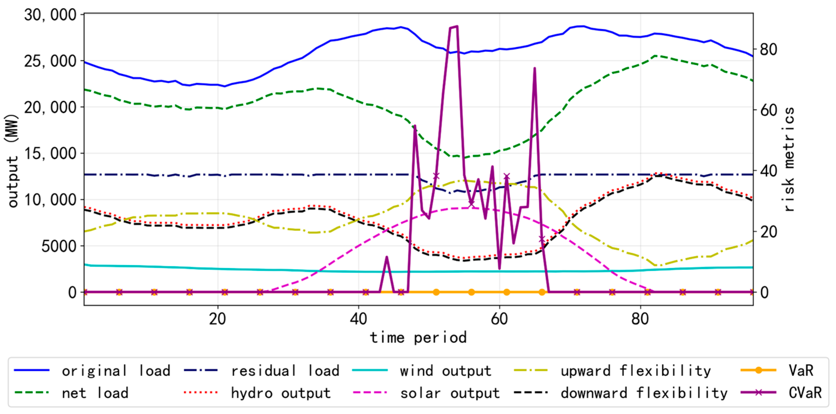
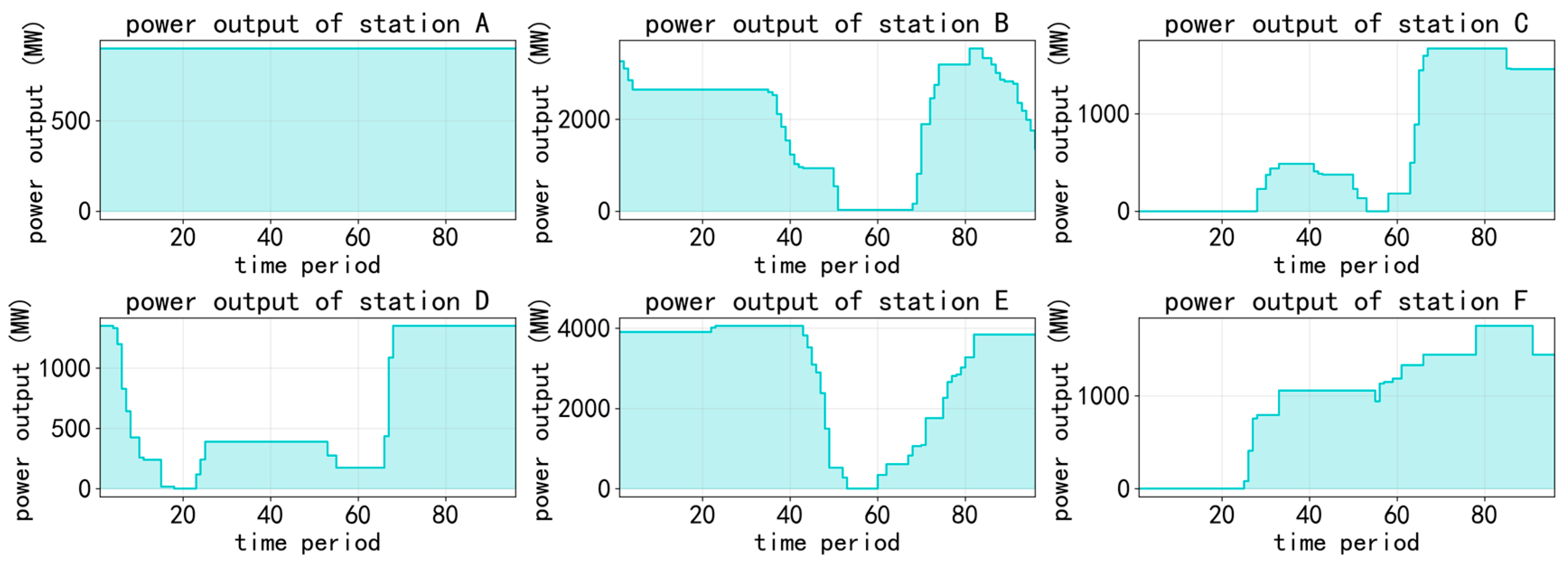
Figure 8 and Figure 9 illustrate the system scheduling results and the output of cascade hydropower stations for the typical dry season day under equal objective weights, while Figure 10 and Figure 11 present the overall system scheduling results and the corresponding hydropower outputs for the typical flood season day.

As shown in Figure 8 and Figure 10, compared with single-objective schemes that either optimize peak shaving or minimize flexibility shortage risk, the equal-weight compromise solution achieves an effective balance between peak-shaving performance and flexibility risk. Specifically, the residual load curve exhibits a characteristic three-stage pattern, namely the pre-noon, midday, and post-noon periods. During the pre-noon and post-noon periods, the residual load remains relatively smooth, whereas significant fluctuations occur around midday. This phenomenon can be attributed to the temporal characteristics of renewable generation and its impact on system flexibility requirements. In the pre-noon and post-noon periods, the combined output of wind and solar output is relatively low, resulting in higher net load with smaller fluctuations. Hydropower can satisfy peak-shaving requirements while maintaining sufficient regulation capability, thereby effectively supporting system peak-shaving and keeping flexibility shortage risk at low levels. In contrast, during midday hours, concentrated solar power generation causes a sharp decline in net load. Although maintaining a smooth residual load would theoretically require a substantial reduction in hydropower output, forecast uncertainty of wind and solar power is also significantly higher during this period, leading to a sharp increase in the demand for downward flexibility. If hydropower output is excessively reduced, it may struggle to respond to extreme scenarios where actual output exceeds forecasts, leading to high flexibility shortfall risks. Consequently, under the compromise strategy that jointly considers peak shaving and flexibility, the dispatch scheme retains a moderate level of hydropower output during midday. While this results in some residual load fluctuations, it effectively mitigates flexibility shortage risk, highlighting the necessity of coordinated multi-objective optimization.

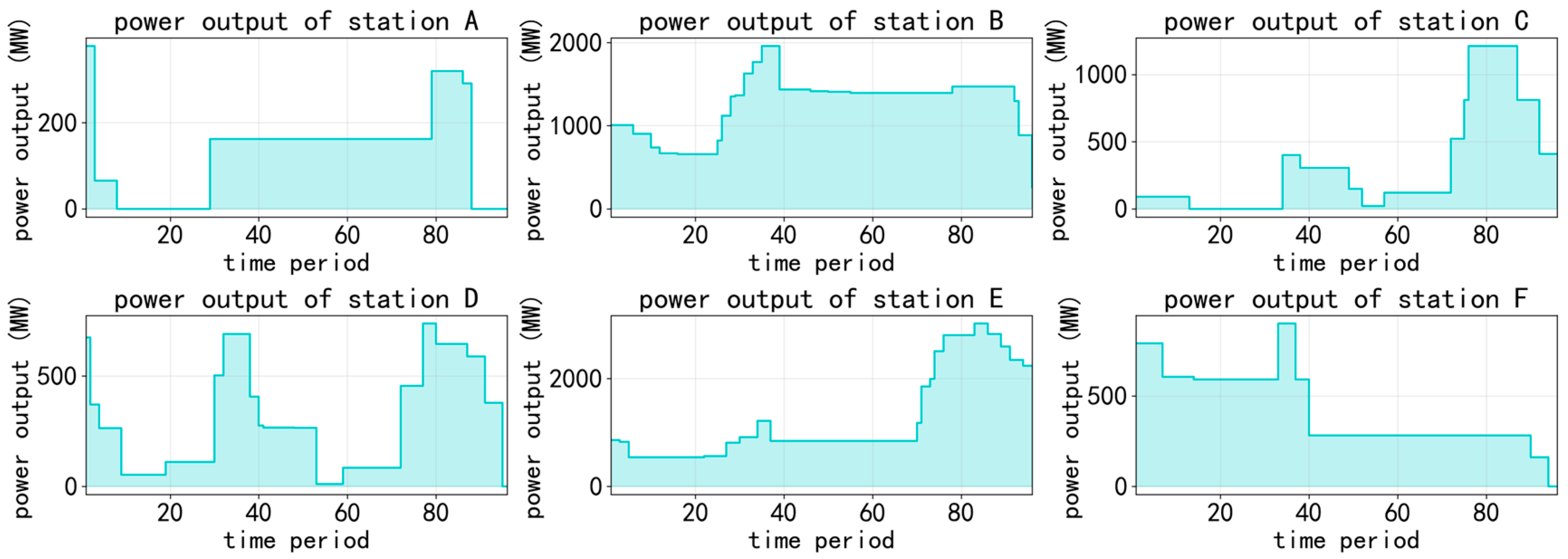
Further analysis of the output of individual hydropower stations (see Figure 9 and Figure 11) reveals that the output of cascade stations mainly focuses on periods with higher net loads, while generally reserving a certain amount of regulation capacity to accommodate the stochastic fluctuations of wind and solar generation and ensure adequate system flexibility. A comparison between flood-season and dry-season scheduling strategies reveals that, owing to abundant inflows during the flood season, all stations except the most upstream Station A—which operates at full output due to limited storage capacity—are able to fully exploit their regulation potential. In particular, downstream stations with strong regulation capability, such as Stations B and E, play a key role, enabling subsequent cascade stations from Station B onward to actively participate in both peak shaving and flexibility support. This coordinated scheduling mechanism based on basin hydrological characteristics, significantly enhances the adaptability of the hydropower system to high proportions of renewable energy integration during the flood season.

4.5. Comparison with Benchmark Models

To quantitatively evaluate the marginal benefits of the proposed CVaR-based multi-objective framework, two benchmark models are introduced for comparison: (1) a stochastic expected-value (EV) model that minimizes the average flexibility shortage across all scenarios without any tail risk measure, and (2) a VaR model that minimizes the α-quantile of the flexibility shortage distribution. All three models share the same peak-shaving objective and the same set of hydropower operational constraints, ensuring a fair comparison.

To ensure computational tractability of the VaR model, which requires binary variables to identify tail scenarios, the original K = 1000 scenarios are reduced to K′ = 100 representative scenarios via K-means clustering. All three models are solved using the NNC method on the same reduced scenario set with J = 25 evenly distributed points along the utopia line. The confidence level is set to α = 0.95 for both CVaR and VaR computations. To comprehensively compare the performance of the three models, five evaluation metrics are adopted. Including peak-valley difference in net load, expected flexibility shortage, VaR, CVaR, maximum flexibility shortage. To ensure a fair and consistent comparison across the three models, all performance metrics reported in this section are computed through a post-optimization simulation procedure rather than directly extracted from the optimization models’ internal variables. Therefore, these post-optimization metrics may differ numerically from the objective function values obtained during optimization. In addition to the metrics introduced above, the expected flexibility shortage and maximum flexibility shortage is calculated as:

(1) Expected flexibility shortage E[L]. The expected flexibility shortage is the average shortage across all time periods and all scenarios:

$$E\left(\mathit{L}\right)={\displaystyle \frac{1}{T}}{\displaystyle \sum _{t = 1}^T}{\displaystyle \frac{1}{K}}{\displaystyle \sum _{k = 1}^K}{L}_{t,k}$$

(2) Maximum flexibility shortage. The maximum flexibility shortage represents the worst-case risk across all scenarios, averaged over all periods, A smaller value indicates higher safety margin under extreme scenarios:

$$L_t^{max}=\underset{k=1,...,K}{\max }{L}_{t,k}$$

$${\overline{L}}^{max}={\displaystyle \frac{1}{T}}{L}_t^{max}$$

In summary, each model directly optimizes a different risk metric. By evaluating all models on the same set of metrics, the comparison reveals the trade-offs inherent in each risk measure.

(1) Typical dry season day

Table 8. Comparison of compromise solutions under different models (typical dry season day).

Model	Peak-Valley (MW)	E[L] (MW)	VaR0.95 (MW)	CVaR0.95 (MW)	${\overline{\mathit{L}}}^{\mathit{m}\mathit{a}\mathit{x}}$ (MW)
CVaR	7670.96	7.40	0.00	7.40	1101.79
EV	6711.47	15.78	72.04	272.34	1212.39
VaR	5591.90	38.44	265.44	460.10	1328.67

summarizes the compromise solution results for the three models under the typical dry season day, evaluated using the equal-weight ideal point method (ω₁ = ω₂ = 0.5).

As shown in Table 8, the EV model achieves the lowest peak-valley difference (6711.47 MW), which is approximately 12.5% lower than that of the CVaR model (7670.96 MW). This indicates that optimizing the average flexibility shortage allows the system to allocate more hydropower capacity toward peak shaving. However, the EV model exhibits significantly higher tail risk: its CVaR reaches 272.34 MW, which is 36.8 times that of the CVaR model (7.40 MW). Similarly, the VaR of the EV model is 72.04 MW, while the CVaR model maintains VaR = 0. The maximum flexibility shortage under the EV model also exceeds that of the CVaR model. These results clearly demonstrate that while the EV model optimizes average performance, it fails to provide adequate protection against extreme scenarios.

(2) Typical flood season day

Table 9. Comparison of compromise solutions under different models (typical flood season day).

Model	Peak-Valley (MW)	E[L] (MW)	VaR0.95 (MW)	CVaR0.95 (MW)	${\overline{\mathit{L}}}^{\mathit{m}\mathit{a}\mathit{x}}$ (MW)
CVaR	1909.60	0.59	0.00	0.59	272.70
EV	1932.04	0.49	0.00	0.49	254.94
VaR	215.92	3.01	0.00	3.01	421.18

summarizes the compromise solution results for the three models under the typical flood season day. In the flood season, the differences among the three models are less pronounced than in the dry season, reflecting the generally lower flexibility shortage risk due to higher hydropower inflows. The CVaR and EV models produce similar compromise solutions, with peak-valley differences of 1909.60 MW and 1932.04 MW, respectively, and both achieve near-zero CVaR values. This similarity arises because the abundant hydropower generation capacity in the flood season allows both models to simultaneously satisfy peak-shaving and risk control requirements to a large extent. The VaR model, however, exhibits a markedly different behavior. Its compromise solution achieves a substantially lower peak-valley difference but at the cost of significantly higher flexibility shortage risk and CVaR. The maximum flexibility shortage also increases to 421.18 MW. This result illustrates a fundamental limitation of VaR as a risk measure: by focusing solely on the quantile threshold, the VaR model does not penalize the severity of tail losses, allowing the optimization to sacrifice tail risk protection in exchange for improved peak-shaving performance.

In summary, the comparison results lead to the following key findings:

(1) The EV model, while achieving competitive or slightly better peak-shaving performance, exhibits substantially higher tail risk. This confirms that optimizing only the expected flexibility shortage is insufficient for ensuring system resilience under extreme scenarios with high renewable uncertainty.

(2) The VaR model minimizes the quantile threshold but fails to control the severity of losses beyond that threshold, resulting in elevated CVaR and maximum flexibility shortage values. This highlights the limitation of VaR as a non-coherent risk measure that does not satisfy subadditivity and cannot fully capture tail risk.

(3) The proposed CVaR model achieves the best overall balance: it provides the strongest tail risk protection while maintaining competitive peak-shaving performance. As a coherent risk measure, CVaR simultaneously controls both the threshold and the expected severity of tail losses, making it the most suitable risk metric for short-term hydro-wind-solar scheduling under high uncertainty.

5. Conclusions

To address the challenges of increasing peak-shaving pressure and operational risk faced by provincial power systems with high penetrations of wind and solar power generation. This paper proposed a bi-objective short-term scheduling model for hydro-wind-solar systems that simultaneously optimizes peak-shaving performance and flexibility shortage risk. Key findings demonstrate that:

(1)

The proposed bi-objective model effectively captures the role of hydropower flexibility in both peak shaving and risk mitigation. System peak-shaving requirement is represented by the maximum net load, while the tail risk of flexibility shortages under extreme scenarios is quantified by the average CVaR of ramping deficits across time periods, thereby overcoming the limitations of traditional single-objective scheduling that neglects the trade-off between operation efficiency and risk.

(2)

The Normalized Normal Constraint method is introduced to derive the Pareto-optimal frontier. Compared with the conventional weighted approach, NNC significantly improves the uniformity and completeness of solution distributions in non-uniform objective spaces, providing decision-makers with high-quality and diverse trade-off solutions. Furthermore, the ideal point method is applied to identify and recommend a representative compromise solution.

(3)

Case studies based on a real-world hydro-wind-solar system in Southwest China demonstrate that the proposed approach achieves excellent peak-shaving performance while effectively controlling flexibility shortage risk under typical dry-season day and flood-season day operating conditions.

In summary, the proposed framework provides theoretical support for the secure, efficient, and resilient operation of provincial hydro-wind-solar complementary systems, and offers practical guidance for short-term power system scheduling, coordinated allocation of flexible resources, and risk-aware operational decision-making. Future work will extend the model to incorporate additional flexibility resources such as energy storage and demand response across multiple time scales, and explore the integration of risk metrics with electricity market mechanisms.

References

1. China’s Wind, Solar Energy Capacity Surpasses Thermal Power for First Time. Available online: https://english.www.gov.cn/archive/statistics/202504/25/content_WS680b7b79c6d0868f4e8f2141.html (accessed on 15 October 2025).
2. National Energy Administration of China. 2025 Grid-Connected Operation of Renewable Energy. Available online: https://www.nea.gov.cn/20260212/742b8c6a078347b0b39de676c05c5d58/c.html (accessed on 24 February 2026).
3. Li, C.; Shah, N.; Li, Z.; Liu, P. Modelling of wind and solar power output uncertainty in power systems based on historical data: A characterisation through deterministic parameters. J. Clean. Prod. 2024, 484, 144233. [Google Scholar] [CrossRef]
4. Liu, B.; Liu, T.; Liao, S.; Lu, J.; Cheng, C. Short-term coordinated hybrid hydro-wind-solar optimal scheduling model considering multistage section restrictions. Renew. Energy 2023, 217, 119160. [Google Scholar] [CrossRef]
5. Xu, Z.; Liu, Q.; Xu, L.; Mo, L.; Zhang, Y.; Zhang, X. Optimal Dispatching Rules for Peak Shaving of Cascaded Hydropower Stations in Response to Large-Scale New Energy Integration. Processes 2025, 13, 612. [Google Scholar] [CrossRef]
6. Shaheen, M.A.M.; Ullah, Z.; Qais, M.H.; Hasanien, H.M.; Chua, K.J.; Tostado-Véliz, M.; Turky, R.A.; Jurado, F.; Elkadeem, M.R. Solution of Probabilistic Optimal Power Flow Incorporating Renewable Energy Uncertainty Using a Novel Circle Search Algorithm. Energies 2022, 15, 8303. [Google Scholar] [CrossRef]
7. Shaheen, M.A.M.; Hasanien, H.M.; Alsaleh, I.; Alassaf, A.; Zhang, M.; Alateeq, A. Optimal power flow in power systems with renewable energy resources uncertainty including geothermal power plants. Ain Shams Eng. J. 2025, 16, 103784. [Google Scholar] [CrossRef]
8. Su, H.; Li, Y.; Zhang, Y.; Wang, Y.; Li, G.; Cheng, C. A Mid-Term Scheduling Method for Cascade Hydropower Stations to Safeguard Against Continuous Extreme New Energy Fluctuations. Energies 2025, 18, 3745. [Google Scholar] [CrossRef]
9. Fan, J.-L.; Huang, X.; Shi, J.; Li, K.; Cai, J.; Zhang, X. Complementary potential of wind-solar-hydro power in Chinese provinces: Based on a high temporal resolution multi-objective optimization model. Renew. Sustain. Energy Rev. 2023, 184, 113566. [Google Scholar] [CrossRef]
10. Wu, X.; Zhang, J.; Wei, X.; Cheng, C.; Cheng, R. Short-Term Hydro-Wind-PV peak shaving scheduling using approximate hydropower output characters. Renew. Energy 2024, 236, 121502. [Google Scholar] [CrossRef]
11. Wang, H.; Liao, S.; Liu, B.; Zhao, H.; Ma, X.; Zhou, B. Long-term complementary scheduling model of hydro-wind-solar under extreme drought weather conditions using an improved time-varying hedging rule. Energy 2024, 305, 132285. [Google Scholar] [CrossRef]
12. Jia, Y.; Xie, M.; Peng, Y.; Wu, D.; Li, L.; Zheng, S. Optimal Configuration and Empirical Analysis of a Wind–Solar–Hydro–Storage Multi-Energy Complementary System: A Case Study of a Typical Region in Yunnan. Water 2025, 17, 2262. [Google Scholar] [CrossRef]
13. Li, J.; Shi, L.; Fu, H. Multi-Objective Short-Term Optimal Dispatching of Cascade Hydro–Wind–Solar–Thermal Hybrid Generation System with Pumped Storage Hydropower. Energies 2024, 17, 98. [Google Scholar] [CrossRef]
14. Zhang, F.; Liu, F.; Chen, L.; Zhang, Y. Integrating day-ahead scheduling and real-time dispatch for hydro-wind-photovoltaic-storage hybrid systems under uncertainties. J. Energy Storage 2026, 141, 119171. [Google Scholar] [CrossRef]
15. Xiong, J.; Liao, S.; Liu, B.; Cheng, C.; Li, S.; Wang, H. A search algorithm that couples physical rules for balancing wind and solar output fluctuations via hydropower in ultra-short-term scheduling. Energy 2025, 330, 136910. [Google Scholar] [CrossRef]
16. Jin, X.; Cheng, C.; Cai, S.; Yan, L.; Zhao, Z. Using stochastic dual dynamic programming to design long-term operation policy of hydro-wind-solar energy systems considering multiple coupled uncertainties and end-of-year carryover storage. Appl. Energy 2025, 393, 126072. [Google Scholar] [CrossRef]
17. Cao, L.; Qian, J.; Zhang, H.; Tian, D.; Mao, X. Capacity Configuration Method for Hydro-Wind-Solar-Storage Systems Considering Cooperative Game Theory and Grid Congestion. Energies 2025, 18, 6543. [Google Scholar] [CrossRef]
18. Zhao, H.; Liao, S.; Liu, B.; Fang, Z.; Wang, H.; Cheng, C.; Zhao, J. Multiagent optimization for short-term generation scheduling in hydropower-dominated hydro-wind-solar supply systems with spatiotemporal coupling constraints. Appl. Energy 2025, 382, 125324. [Google Scholar] [CrossRef]
19. Li, Y.; Kong, F.; Jing, C.; Yang, L. MILP model for peak shaving in hydro-wind-solar-storage systems with uncertainty and unit commitment. Electr. Power Syst. Res. 2025, 241, 111358. [Google Scholar] [CrossRef]
20. Shi, Y.; Li, C.; Wang, H.; Wang, X.; Negnevitsky, M. A novel scheduling strategy of a hybrid wind-solar-hydro system for smoothing energy and power fluctuations. Energy 2025, 320, 135268. [Google Scholar] [CrossRef]
21. Liu, B.; Liu, T.; Liao, S.; Wang, H.; Jin, X. Short-term operation of cascade hydropower system sharing flexibility via high voltage direct current lines for multiple grids peak shaving. Renew. Energy 2023, 213, 11–29. [Google Scholar] [CrossRef]
22. Zhu, F.; Zhao, L.; Liu, W.; Zhu, O.; Hou, T.; Li, J.; Guo, X.; Zhong, P. A stochastic optimization framework for short-term peak shaving in hydro-wind-solar hybrid renewable energy systems under source-load dual uncertainties. Appl. Energy 2025, 400, 126597. [Google Scholar] [CrossRef]
23. Zhao, G.; Yu, C.; Huang, H.; Yu, Y.; Zou, L.; Mo, L. Optimization Scheduling of Hydro–Wind–Solar Multi-Energy Complementary Systems Based on an Improved Enterprise Development Algorithm. Sustainability 2025, 17, 2691. [Google Scholar] [CrossRef]
24. Ming, B.; Chen, J.; Fang, W.; Liu, P.; Zhang, W.; Jiang, J. Evaluation of stochastic optimal operation models for hydro–photovoltaic hybrid generation systems. Energy 2023, 267, 126500. [Google Scholar] [CrossRef]
25. Pan, L.; Xu, X.; Yang, Y.; Liu, J.; Hu, W. Distributionally robust economic scheduling of a hybrid hydro/solar/pumped-storage system considering the bilateral contract flexible decomposition and day-ahead market bidding. J. Clean. Prod. 2023, 428, 139344. [Google Scholar] [CrossRef]
26. Liu, B.; Lund, J.R.; Liao, S.; Jin, X.; Liu, L.; Cheng, C. Optimal power peak shaving using hydropower to complement wind and solar power uncertainty. Energy Convers. Manag. 2020, 209, 112628. [Google Scholar] [CrossRef]
27. Huang, H.; Shen, Q.; Liu, W.; Peng, Y.; Zhu, S.; Bao, R.; Mo, L. Optimal Scheduling of a Hydropower–Wind–Solar Multi-Objective System Based on an Improved Strength Pareto Algorithm. Sustainability 2025, 17, 7140. [Google Scholar] [CrossRef]
28. Xu, Y.; Jiang, Z.; Peng, W.; Lu, P.; Wang, J.; Xu, Y.; Lu, J. Multi-objective optimization and mechanism analysis of integrated hydro-wind-solar-storage system: Based on medium-long-term complementary dispatching model coupled with short-term power balance. Energy 2025, 332, 137246. [Google Scholar] [CrossRef]
29. Zhou, S.; Han, Y.; Zalhaf, A.S.; Chen, S.; Zhou, T.; Yang, P.; Elboshy, B. A novel multi-objective scheduling model for grid-connected hydro-wind-PV-battery complementary system under extreme weather: A case study of Sichuan, China. Renew. Energy 2023, 212, 818–833. [Google Scholar] [CrossRef]
30. Wang, K.; Zhu, H.; Dang, J.; Ming, B.; Wu, X. Short-term optimal scheduling of wind-photovoltaic-hydropower-thermal-pumped hydro storage coupled system based on a novel multi-objective priority stratification method. Energy 2024, 309, 133190. [Google Scholar] [CrossRef]
31. Ju, L.; Li, P.; Tan, Q.; Tan, Z.; De, G. A CVaR-Robust Risk Aversion Scheduling Model for Virtual Power Plants Connected with Wind-Photovoltaic-Hydropower-Energy Storage Systems, Conventional Gas Turbines and Incentive-Based Demand Responses. Energies 2018, 11, 2903. [Google Scholar] [CrossRef]
32. Jia, Y.; Xia, B.; Shi, Z.; Chen, W.; Zhang, L. Distributed Risk-Averse Optimization Scheduling of Hybrid Energy System with Complementary Renewable Energy Generation. Energies 2025, 18, 1405. [Google Scholar] [CrossRef]
33. Sánchez de la Nieta, A.A.; Contreras, J.; Catalão, J.P.S. Impact of the future water value on wind-reversible hydro offering strategies in electricity markets. Energy Convers. Manag. 2015, 105, 313–327. [Google Scholar] [CrossRef]
34. Wu, J.; Zhang, B.; Li, H.; Li, Z.; Chen, Y.; Miao, X. Statistical distribution for wind power forecast error and its application to determine optimal size of energy storage system. Int. J. Electr. Power Energy Syst. 2014, 55, 100–107. [Google Scholar] [CrossRef]
35. Ogunniran, O.; Babatunde, O.; Akintayo, B.; Adisa, K.; Ighravwe, D.; Ogbemhe, J.; Olanrewaju, O.A.; Ogunniran, O.; Babatunde, O.; Akintayo, B.; et al. Risk-Based Optimization of Renewable Energy Investment Portfolios: A Multi-Stage Stochastic Approach to Address Uncertainty. Appl. Sci. 2025, 15, 2346. [Google Scholar] [CrossRef]
36. Liu, Y.; Zhang, X.; Ma, Z.; Ren, W.; Xiao, Y.; Xu, X.; Liu, Y.; Liu, J.; Liu, Y.; Zhang, X.; et al. Risk-Aware Scheduling for Maximizing Renewable Energy Utilization in a Cascade Hydro–PV Complementary System. Energies 2025, 18, 3109. [Google Scholar] [CrossRef]
37. Liu, Z.; Tan, Q.; Huang, R.; Wang, Z.; Wen, X. Short-term peak-shaving strategies for cascade hydropower against evolving net load in systems with high VRE penetration. Renew. Energy 2026, 267, 125773. [Google Scholar] [CrossRef]
38. Cheng, J.; De Waele, W. Multi-objective weighted average algorithm: A novel algorithm for multi-objective optimization problems and its application in engineering problems. Eng. Appl. Artif. Intell. 2025, 159, 111569. [Google Scholar] [CrossRef]
39. Zhang, Q.; Xie, Z.; Lu, M.; Ji, S.; Liu, D.; Xiao, Z.; Zhang, Q.; Xie, Z.; Lu, M.; Ji, S.; et al. Optimization of Hydropower Unit Startup Process Based on the Improved Multi-Objective Particle Swarm Optimization Algorithm. Energies 2024, 17, 4473. [Google Scholar] [CrossRef]
40. Liu, B.; Peng, Z.; Liao, S.; Liu, T.; Lu, J. A multi-objective optimization model for the coordinated operation of hydropower and renewable energy. Front. Energy Res. 2023, 11, 1193415. [Google Scholar] [CrossRef]
41. Messac, A.; Ismail-Yahaya, A.; Mattson, C.A. The normalized normal constraint method for generating the Pareto frontier. Struct. Multidiscip. Optim. 2003, 25, 86–98. [Google Scholar] [CrossRef]
Figure 1. System results for the typical dry season day considering peak shaving only.
Energies 19 03272 g001
Figure 2. System results for the typical dry season day considering flexibility shortage risk.
Energies 19 03272 g002
Figure 3. System results for the typical flood season day considering peak shaving only.
Energies 19 03272 g003
Figure 4. System results for the typical flood season day considering flexibility shortage risk.
Energies 19 03272 g004
Figure 5. Pareto fronts obtained by different methods for the typical dry-season day. (a) Weighted method. (b) NNC method.
Energies 19 03272 g005
Figure 6. Pareto fronts obtained by different methods for the typical flood-season day. (a) Weighted method. (b) NNC method.
Energies 19 03272 g006
Figure 7. Pareto fronts and compromise solutions under typical weight settings. (a) Typical dry-season day. (b) Typical flood-season day.
Energies 19 03272 g007
Figure 8. System results for the typical dry-season day under equal objective weights.
Energies 19 03272 g008
Figure 9. Output of hydropower stations for the typical dry-season day under equal objective weights.
Energies 19 03272 g009
Figure 10. System results for the typical flood-season day under equal objective weights.
Energies 19 03272 g010
Figure 11. Output of hydropower stations for the typical flood-season day under equal objective weights.
Energies 19 03272 g011