XGBoost-Guided Spectrogram Pruning with SE-Augmented Residual CNN for Wind Turbine Gearbox Fault Diagnosis Under Unsteady Conditions

Abstract

Reliable condition monitoring of wind turbine gearboxes is critical to reducing unplanned downtime and maintenance costs in wind farms. However, this task presents significant challenges due to the non-stationary nature of vibration signals, in which fault-relevant features are sparsely and unevenly distributed across the time–frequency map. Although time–frequency analysis has been widely adopted to represent nonlinear and non-stationary vibration signals, existing deep learning methods typically process the full spectrogram directly, without distinguishing redundant or uninformative regions. This leads to high input dimensionality and exposes the model to substantial spectral noise. Consequently, it increases computational burden and potentially reduces the diagnostic reliability. To address this issue, this paper proposes a two-stage hybrid framework based on complementary selection mechanisms operating on two distinct feature spaces. In the first stage, eXtreme Gradient Boosting (XGBoost) importance scores are used to identify and permanently prune uninformative time–frequency features from the input spectrogram, reducing the input map size by 25%. In the second stage, a Squeeze-and-Excitation (SE) block, inserted after the deepest residual layer, performs soft channel-wise recalibration of the abstract feature maps produced by the residual convolutional neural network (ResCNN), thereby amplifying discriminative representations prior to classification. The proposed method was evaluated in an eight-class variable-speed fault classification task using the MCC5-THU benchmark, where data were collected from a 2.2 kW motor-driven gearbox test rig. The proposed method achieves a mean accuracy of 97.81% ± 0.33% under 5-fold stratified cross-validation (CV), while reducing classifier training time by approximately 23% compared to a baseline model trained on the full spectrogram. These results demonstrate that explicit input-level spectrogram pruning, combined with model-level channel attention, yields a robust and computationally efficient diagnostic framework for wind turbine gearbox condition monitoring.

1. Introduction

Wind turbines are central to modern large-scale renewable energy generation, but their operational reliability is often compromised by mechanical degradation in the drivetrain [1]. Among the most failure-prone and maintenance-intensive components in the drivetrain is the gearbox, which transmits torque from the low-speed rotor shaft to the high-speed generator shaft [2]. Gearbox failures account for a disproportionate share of wind turbine downtime. Moreover, repair or replacement frequently requires crane mobilization at remote onshore or offshore sites, causing the associated costs to far exceed the value of the component itself [3]. Consequently, reliable and timely fault detection in wind turbine gearboxes is economically critical. Early identification of incipient faults enables condition-based maintenance scheduling, which reduces unplanned shutdowns and mitigates the risk of secondary damage propagation [4]. Vibration-based condition monitoring has emerged as the dominant methodology for wind turbine gearbox monitoring, as vibration signals are highly sensitive to localized mechanical anomalies such as gear pitting, tooth cracking, and bearing race defects [5].

A central challenge in vibration-based wind turbine gearbox monitoring is that wind turbines rarely operate at steady speeds [6]. Grid frequency fluctuations, variable wind loading, and power regulation strategies all produce continuously varying shaft speed profiles, rendering operating conditions inherently non-stationary [7,8]. Fixed-frequency analysis tools such as the Discrete Fourier Transform fail to capture this temporal evolution, prompting the development of various time–frequency representations, including the Short-time Fourier Transform (STFT), the Continuous Wavelet Transform (CWT), and the Wigner-Ville Distribution (WVD), among others [9]. Among these, STFT spectrograms have seen widespread adoption in deep learning-based fault diagnosis, as they generate structured two-dimensional time–frequency maps that are computationally efficient to produce and directly compatible with convolutional architectures [10]. However, a structural limitation in how deep learning models consume these representations has received surprisingly little systematic attention.

In a gearbox vibration spectrogram, fault-relevant features are not distributed uniformly across the time–frequency map. Gear mesh harmonics, modulation sidebands, and bearing defect frequencies typically appear in specific frequency regions that are physically interpretable to domain experts. In contrast, the remaining regions may contain background vibration, sensor noise, broadband structural resonances, and other patterns whose discriminative value is less directly interpretable [11]. Existing deep learning methods typically feed the full time–frequency map directly into a convolutional network [12,13]. The network then converts the map into abstract feature representations through a sequence of learned spatial transformations. This process implicitly relies on the network to internally disregard uninformative features, without any explicit prior guidance on which features or time–frequency regions on the map are diagnostically relevant. Consequently, the model must process a larger input, exposing the early convolutional layers to more irrelevant activation patterns and increasing the burden on feature learning.

A related but structurally distinct challenge arises at the level of the network’s learned representations. After the convolutional backbone encodes the input spectrogram into deep feature maps, not all feature channels carry equal discriminative weight for a given fault class. Several feature recalibration mechanisms have been developed to address this issue, including SE networks for channel-wise recalibration [14], spatial SE mechanisms for spatial feature re-weighting [15], and combined variants such as the Convolutional Block Attention Module (CBAM) [16]. These mechanisms learn adaptive weights that modulate the contribution of individual feature channels or spatial locations before classification, thereby emphasizing discriminative representations and suppressing less informative ones. Such mechanisms have been applied to fault diagnosis in several prior studies [17,18,19]. However, these works uniformly operate on full, unpruned input representations and do not clarify whether latent-level recalibration provides an additional benefit after signal-level redundancy has been removed.

To address both the aforementioned challenges, this paper proposes a two-stage hybrid framework through selection mechanisms designed to operate on fundamentally different feature spaces. In Stage 1, XGBoost gain-based importance scores computed from the raw STFT spectrogram pixels are used to permanently discard uninformative time–frequency features before any neural processing, constituting a hard, irreversible selection in the interpretable time–frequency domain. In Stage 2, a channel attention block inserted after the deepest residual layer performs soft, continuous re-weighting of the abstract CNN feature maps, amplifying discriminative channels and suppressing weaker ones before classification. Together, these two complementary stages address redundancy at the input level and refine the model’s internal representation in the latent feature space. 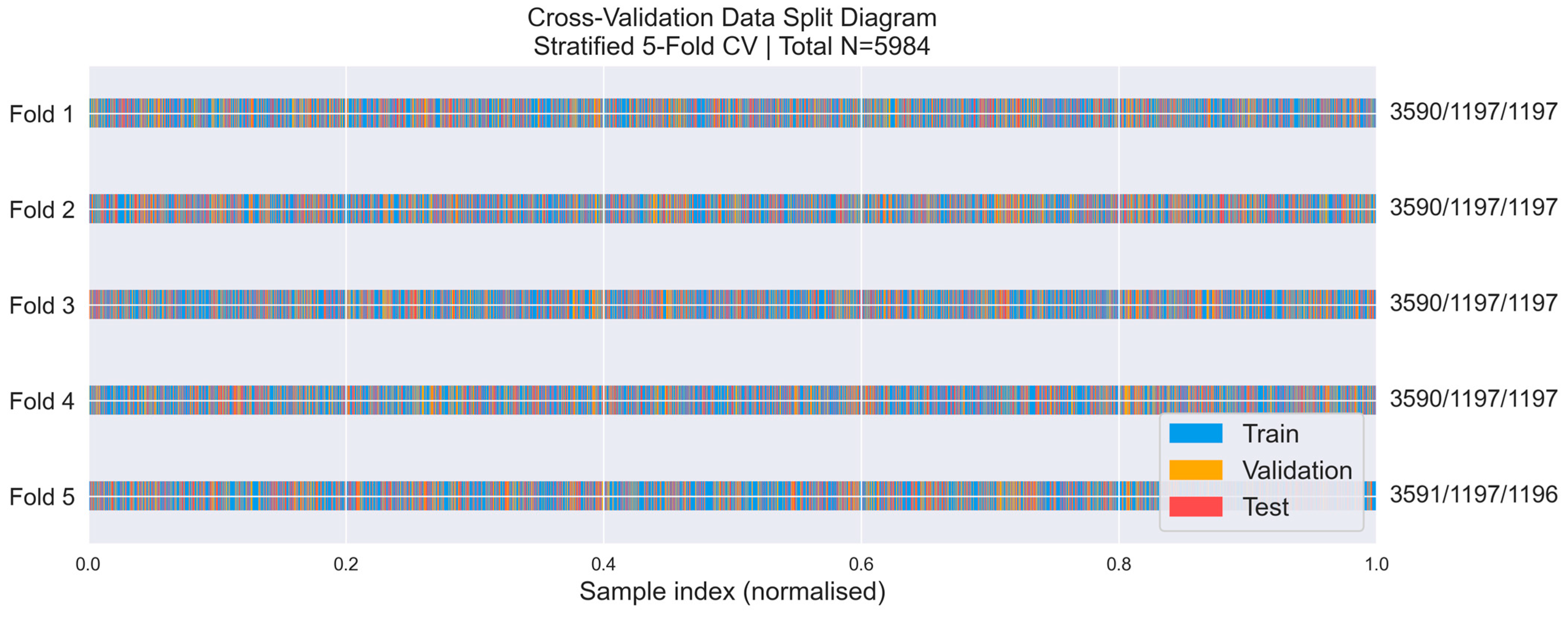The framework is evaluated on the publicly available MCC5-THU parallel gearbox benchmark under a variable-speed [20], eight-class gearbox condition classification setting. This benchmark contains multiple single faults, compound faults, and a healthy baseline, enabling evaluation across a broad range of gearbox health conditions. It also incorporates variable-speed and variable-load operating regimes, while providing sufficiently long and comparable recordings for consistent sample generation. In addition, the availability of triaxial vibration measurements supports spectrogram-based gearbox fault diagnosis under unsteady operating conditions. The performance of the proposed method is assessed through 5-fold stratified CV.

The contributions of this paper are as follows. First, a two-stage, dual-domain selection framework is proposed to integrate input-level spectrogram pruning and latent-level channel recalibration within a single diagnostic pipeline, addressing two limitations that existing methods leave unresolved together. Second, XGBoost gain-based importance scoring is applied as a preprocessing pixel selector operating directly on raw STFT spectrogram maps, a use that is distinct from prior applications of XGBoost in fault diagnosis, which employ it as a standalone classifier or scorer of hand-crafted features. Third, the proposed framework systematically examines the interaction between signal-level spectrogram pruning and latent-level feature recalibration within a unified pipeline. It further investigates how the choice of recalibration mechanism and its insertion depth within the residual backbone affect the effectiveness of the combined design.

The remainder of this paper is organized as follows. Section 2 reviews related work. Section 3 presents the proposed methodology. Section 4 describes the experimental setup and evaluation protocol. Section 5 reports and discusses the results. Section 6 concludes the paper.

2. Related Work

Vibration-based condition monitoring has long been a central approach for detecting gearbox faults, but its effectiveness, to a large extent, depends on the operating regime. Under stationary or near-stationary operating conditions, fault-characteristic frequencies are well localized in the spectrum, and classical frequency-domain methods are highly effective. In [21], the authors use envelope-spectrum analysis to extract frequency-domain fault features, illustrating the effectiveness of classical demodulation-based diagnosis under stationary or near-stationary conditions. Under more complex operating conditions, fault-characteristic frequencies no longer remain confined to fixed spectral locations. Therefore, purely frequency-domain analysis may become less effective. For example, when the rotational speed is no longer stationary, angular-resampling approaches can be used to convert the vibration signal into the angular domain, thereby restoring a constant number of samples per revolution. In [22], the authors combine encoder-based angular resampling with order-spectrum features and a Support Vector Machine (SVM) classifier, although this method relies on external speed measurement. A more general alternative for handling complex signal conditions, including variable speed, noisy environments, and changing operating regimes, is to represent the signal in a time–frequency domain. In [23], the authors apply the CWT to triaxial gearbox vibration to localize short-duration phenomena in vibration signals, although the resulting representation still depends on wavelet-design choices. Among time–frequency representations, the STFT has become a widely used front end for vibration-based fault diagnosis, especially when temporal variation in the signal is important. In [24], the authors use a logarithmic STFT to construct a physically interpretable time–frequency map for wheelset-bearing diagnosis under time-variable speed and load, feeding it into a modified self-calibrated residual network. Once the vibration signal has been mapped to a two-dimensional time–frequency image, the diagnosis task naturally reshapes into an image-classification problem, opening the door to deep convolutional models.

Building on this image-based formulation, CNNs have become a widely used backbone for time–frequency-image-based fault classification, with architectures progressing from shallow CNNs to deeper residual and hybrid designs. In [25], the authors use STFT to convert bearing vibration into two-dimensional spectrum maps and train a Visual Geometry Group (VGG) style CNN directly on these images for fault classification. To improve robustness, deeper residual backbones have since been adopted. In [26], the authors propose an improved residual network (ResNet) trained on wavelet time–frequency images of bearing vibration, demonstrating stronger robustness to noise than plain CNN baselines and confirming the benefit of residual connections for deep learning on time–frequency image-based fault diagnosis. To better capture fault patterns distributed at different spectral–temporal scales, multi-scale designs have also been introduced. In [12], the authors propose a multi-scale CNN in which parallel convolutional branches operating at different receptive fields are combined through depth-wise feature concatenation, preserving complementary local and global information from STFT spectrograms of gearbox vibration. More recently, Transformer-based fusion components have been incorporated to model global dependencies that are difficult to capture with purely local convolutions. In [27], the authors develop a hybrid model in which a time-domain branch and a STFT-based time–frequency branch are fused through a Transformer encoder, modeling long-range and cross-domain interactions across the two feature streams. Across these approaches, the time–frequency representation is fed into the network in its entirety, and the task of distinguishing discrimination from uninformative regions is left implicit to the convolutional or self-attention layers. No explicit pruning of the input is performed before feature extraction, so every region, informative or not, still contributes to the early feature representation and its associated computation.

There are some studies that reduce the vibration representation before classification, but most of these methods still operate on predefined frequency regions or engineered descriptors rather than on raw time–frequency coordinates. In [28], the authors define feature sets based on frequency bands centered on gear-mesh harmonics and their sidebands, and use the resulting band powers or peak amplitudes as inputs to machine learning models. This keeps the input physically interpretable, but the retained regions are determined by prior fault knowledge rather than by what the classifier itself finds most discriminative, so potentially useful frequency information outside the predefined bands may be ignored. In [29], the authors use spectral kurtosis to identify the demodulation band with the strongest impulsive content for envelope analysis. Compared with manual band definition, this provides a more adaptive way of isolating transients, but the selection is still driven by signal statistics rather than by diagnostic class separability. In [30], the authors apply maximum relevance minimum redundancy (mRMR) to select discriminative features from a fused feature set comprising handcrafted time-domain and frequency-domain statistics together with CNN-extracted local features, before SVM classification. Although this introduces feature selection before classification, the selection is still performed on engineered or learned descriptors derived from the signal, rather than directly on the original spectrum or spectrogram coordinates. A similar pattern appears in [31], where tree-based importance is used to analyze the contribution of engineered vibration features to diagnosis performance. In [32], the authors use XGBoost as the final classifier on extracted vibration descriptors, showing that tree ensembles can perform well on low-dimensional hand-crafted inputs. However, across these studies, tree-based ranking or classification is mainly applied after feature engineering, not to the raw STFT map itself. A closer step toward direct spectral selection was reported in [33], where XGBoost was used to identify discriminative frequency bands for wind turbine drivetrain fault diagnosis before CNN–Transformer classification. However, this method was limited to one-dimensional frequency-domain selection under constant-speed conditions; the selected representations were confined to spectral components and could not capture localized time–frequency patterns. It therefore did not address the redundancy of time–frequency representations under variable-speed operation. As a result, interpretable pruning of individual time–frequency pixels before deep feature extraction remains largely underexplored.

A further line of research addresses the fact that a plain CNN treats all learned feature channels equally by introducing attention mechanisms that re-weight latent features adaptively during training. In [34], the authors combine symmetrized-dot-pattern (SDP) images with an SE-augmented CNN, where the SE mechanism re-weights the feature channels prior to the classification head and suppresses redundant activations. A more expressive variant is explored in [35], where the authors combine channel and spatial attention through a CBAM integrated into a CNN trained on time–frequency images of bearing vibration, with channel attention emphasizing informative feature maps and spatial attention highlighting discriminative regions within each map. Efficiency has also been a driver of recent designs. In [36], the authors adopted Efficient Channel Attention (ECA) in the last two layers of a depth-wise separable CNN, using a lightweight channel-attention mechanism to reduce parameter count while retaining channel-level adaptivity. More recently, Transformer-based designs have been introduced in the literature. In [37], the authors develop a time–frequency dual-channel Transformer in which self-attention captures long-range dependencies that local convolutions struggle to represent, while a multi-scale feature extraction module preserves local spectral–temporal structure. In every case, the attention mechanism operates on feature maps produced by earlier feature-extraction layers, which are abstract learned representations with no direct correspondence to specific frequency bins or time frames. Attention therefore performs a soft, continuous re-weighting in the latent feature space, but by construction it cannot remove redundancy at the input level, because the input has already been consumed by the time the attention layer is reached.

Across these four strands, reducing redundancy in the time–frequency representation and re-weighting features according to their discriminative contribution have developed largely as separate efforts. On the one hand, signal-level reduction methods either confine themselves to predefined frequency regions derived from prior fault knowledge or apply ranking only after the vibration signal has already been transformed into engineered descriptors. In neither case is the selection decision exercised directly over the raw time–frequency image itself. On the other hand, attention-based models improve diagnosis by adaptively re-weighting latent features after the full spectrogram has entered the network, but they do not remove redundancy at the input level because the original map has already been consumed by the time the attention mechanism is applied. As a result, the literature has not yet clearly addressed whether discriminative time–frequency features can be selected directly from the spectrogram in an interpretable and class-relevant manner before deep feature extraction, nor whether such signal-level pruning remains beneficial when combined with channel-level re-weighting in the latent feature space. This unresolved combination defines the research gap that the present work aims to address.

3. Proposed Methodology

3.1. Overview

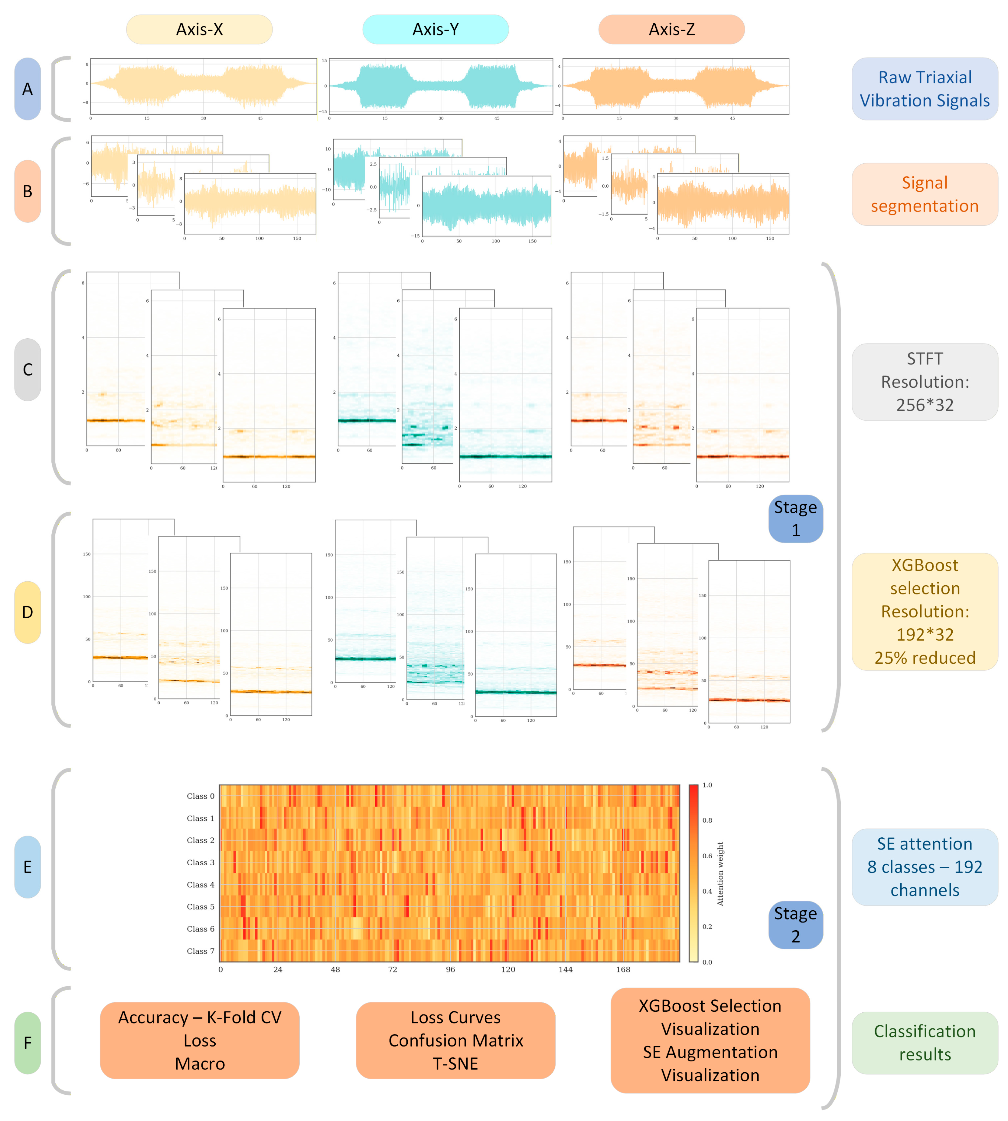
To fill the knowledge gap identified above, we propose a dual-domain hard–soft selection framework for vibration-based gearbox fault classification in this section. It combines two structurally distinct selection mechanisms that operate sequentially on complementary feature spaces. The overall pipeline of the proposed framework is illustrated in Figure 1.

The framework comprises two selectors that differ fundamentally in both the type of selection performed and the feature spaces they act upon. The first is a hard selector, in which an XGBoost classifier is trained directly on an STFT spectrogram, the interpretable time–frequency representation that a domain expert would inspect, and uses gain-based feature importance to permanently discard uninformative time–frequency locations, producing a compact reduced spectrogram. This selection is irreversible; the removed features will play no further role in the pipeline. The second is a soft selector, in which a Squeeze-and-Excitation block placed at the deepest stage of a residual CNN operates on abstract learned channel feature maps that have no direct spectral interpretation. Rather than removing information from maps, it computes a continuous attention weight for each feature channel and uses these weights to re-scale the channel activations, so that the embedding passed to the classifier reflects the relative discriminative contribution of each channel.

3.2. Signal Representation

The raw input consists of vibration signals collected simultaneously along three orthogonal axes by sensors mounted on the gearbox. To convert this into a structured, two-dimensional representation suitable for machine learning, each signal is first segmented using a sliding window approach. Given the $i$-th segment signal $x_i$,

$$x_i=x\left[iS+1,iS+2,\dots ,iS+L \right],\hspace{1em}\hspace{1em}i=0, \dots , \left[{\displaystyle \frac{N_{sig}-L}{S}}\right]$$

(1)

where $i$ refers to segment index, $L$ is the number of samples in the segmented signal, $N_{sig}$ is the total number of data points in the raw signal, and $S$ is the stride of the window sliding along the time axis. Adjacent windows will overlap when $S<L$, which increases the number of training samples obtained from the continuous vibration signal.

Each segmented signal $x_i$ is converted into a time–frequency spectrogram using the STFT, which operates by sliding a short window of length $N_w$, across the segment signal with a hop size of $H$ samples between adjacent frames, computing the Discrete Fourier Transform (DFT) at each position. For the segment $x_i$, the STFT coefficient at time frame $m$ and frequency bin $k$ is defined as [38]:

$$X_i\left[m,k\right]={\displaystyle \sum _{n=0}^{N_w-1}}{x}_i[n+mH]·w\left[n\right]·e^{-j2\pi kn/N_{fft}}$$

(2)

where $m=0, \dots , T-1$; $k=0, \dots , N_{fft}/2$, $T$ is the number of time frames, $w\left[n\right]$ is a Hann window of length $N_w$, and $N_{fft}$ is the FFT size controlling the frequency resolution. The magnitude spectrogram $S_i\left[m,k\right]=\left|X_i\left[m,k\right]\right|$ is then obtained by taking the absolute value of the complex STFT coefficients.

The output dimensions of the spectrogram are computed directly from the STFT parameters, without any interpolation or resizing. For a one-sided transform, the number of frequency bins F after removing the zero-frequency component at $k=0$ is $F=N_{fft}/2$, and the number of time frames T is [39]:

$$T=\left[{\displaystyle \frac{L-N_w}{H}}\right]+1$$

(3)

By selecting $L$, $N_w$, $H$ and $N_{fft}$, the spectrogram dimensions are fixed by construction.

This process is applied independently to each of the three vibration signal axes, producing magnitude spectrograms $S_i^{\left(c\right)}\in {\mathbb{R}}^{F\times T}$ for $c\in \left\{\mathrm{1,2},3\right\}$ corresponding to the x, y, and z axes, respectively. The three spectrograms are concatenated along the channel dimension to form a multi-channel tensor of shape $F\times T\times 3$ (frequency bins $\times$ time frames $\times$ channels), which serves as the input to Stage 1 of the proposed pipeline in Figure 1. Then, the reduced representation produced by Stage 1 is passed to Stage 2, as described in the following sections.

3.3. Stage 1—XGBoost Hard Selection

The multi-channel spectrogram samples produced in Section 3.2 serve as the input to Stage 1. While the STFT spectrogram is a compact and interpretable representation of the vibration signal, not all time–frequency components in the spectrogram carry discriminative information for fault classification. The purpose of Stage 1 is to address this issue by applying an XGBoost classifier to the spectrogram pixels to identify and permanently remove those that contribute little to classification, producing a streamlined spectrogram that is passed to Stage 2.

To construct the input feature vector for XGBoost, the pixels from all three channel spectrograms $S_i^{\left(c\right)}[m,k]$ are extracted in order and concatenated sequentially into a single one-dimensional feature vector:

$$z_i=\left[vec\left(S_i^{\left(1\right)}\right),vec\left(S_i^{\left(2\right)}\right),vec\left(S_i^{\left(3\right)}\right)\right]$$

(4)

where $vec\left(S_i^{\left(c\right)}\right)\in {\mathbb{R}}^{F\times T}$ is the row-major flattening of channel $c$. The resulting vector $z_i\in {\mathbb{R}}^{3\times F\times T}$ contains all pixels from all three channels, concatenated in channel order, so that the pixels of each channel form a continuous block of length $F\times T$ within $z_i$.

XGBoost is an ensemble method based on gradient-boosted decision trees that builds a strong predictor $\widehat{y}$ as an additive combination of $R$ weak learners [40]:

$$\widehat{y}={\displaystyle \sum _{r=1}^R}{f}_r\left(z_i\right)$$

(5)

where $f_r\in \mathcal{F}$, $\mathcal{F}$ is the space of regression tree functions, $f_r$ is the $r$-th tree, and $R$ is the total number of trees. Training minimizes a regularized objective $\mathcal{L}$ combining the empirical loss $\mathcal{l}$ and a complexity penalty $\Omega$:

$$\mathcal{L}={\displaystyle \sum _{n=1}^{N_{tr}}}\mathcal{l}\left(y_n, {\widehat{y}}_n\right)+{\displaystyle \sum _{r=1}^R}\Omega \left(f_r\right)$$

(6)

where $N_{tr}$ is the number of training samples, $y_n$ is the true class label for sample $n$, and ${\widehat{y}}_n$ is the corresponding predicted output. The regularization term penalizes overly complex trees and helps reduce over-fitting.

The model is trained in an additive manner, where new trees are introduced sequentially to reduce the residual errors of the ensemble constructed so far. For the present multi-class fault classification task with Q classes, the empirical loss is written in the multi-class cross-entropy form:

$$\mathcal{l}\left(y_n, {\widehat{y}}_n\right)=-{\displaystyle \sum _{q=1}^Q}{y}_{n,q}\mathrm{l}\mathrm{o}\mathrm{g}\left(p_{n,q}\right)$$

(7)

where $y_{n,q}$ is a binary label indicating whether sample $n$ belongs to class $q$, and $p_{n,q}$ is the predicted probability that sample $n$ belongs to class $q$, obtained from the class-wise raw outputs. In the proposed framework, however, XGBoost is not used as the final fault classifier. Instead, it is employed only as an auxiliary supervised model for estimating the discriminative contribution of individual spectrogram pixels.

At each internal node of a decision tree, XGBoost selects the split that maximizes the reduction in the objective function, referred to as the gain:

$$\mathrm{G}\mathrm{a}\mathrm{i}\mathrm{n}={\displaystyle \frac{1}{2}}\left[{\displaystyle \frac{{\left(G_L^{\mathrm{x}\mathrm{g}\mathrm{b}}\right)}^2}{H_L^{\mathrm{x}\mathrm{g}\mathrm{b}}+\lambda }}+{\displaystyle \frac{{\left(G_R^{\mathrm{x}\mathrm{g}\mathrm{b}}\right)}^2}{H_R^{\mathrm{x}\mathrm{g}\mathrm{b}}+\lambda }}-{\displaystyle \frac{{\left(G_L^{\mathrm{x}\mathrm{g}\mathrm{b}}+G_R^{\mathrm{x}\mathrm{g}\mathrm{b}}\right)}^2}{H_L^{\mathrm{x}\mathrm{g}\mathrm{b}}+H_R^{\mathrm{x}\mathrm{g}\mathrm{b}}+\lambda }}\right]-\gamma$$

(8)

where $G_L^{\mathrm{x}\mathrm{g}\mathrm{b}}$ and $G_R^{\mathrm{x}\mathrm{g}\mathrm{b}}$ are the sums of first-order gradient statistics for the left and right branches, respectively, $H_L^{\mathrm{x}\mathrm{g}\mathrm{b}}$ and $H_R^{\mathrm{x}\mathrm{g}\mathrm{b}}$ are the sums of second-order gradient statistics, $\lambda$ is the leaf-weight regularization term, and $\gamma$ is the complexity penalty for introducing a new leaf. A larger gain indicates that the corresponding split leads to a greater reduction in training loss and therefore that the associated input feature is more useful for classification. The gain-based importance score $I^{\left(c\right)}\left(p\right)$ for pixel $p$ in channel $c$ is obtained by accumulating the gain across all nodes and all trees where that pixel is used as the splitting feature:

$$I^{\left(c\right)}\left(p\right)={\displaystyle \sum _{r=1}^R}\sum _{t\in {\mathcal{F}}_r(p,c)}\mathrm{G}\mathrm{a}\mathrm{i}\mathrm{n}\left(t\right)$$

(9)

where ${\mathcal{F}}_r(p,c)$ denotes the set of nodes in tree ${\mathcal{F}}_r$ at which pixel $p$ from channel $c$ is used for splitting, and $t$ indexes a split node. A high value of $I^{\left(c\right)}\left(p\right)$ indicates that pixel $p$ in channel $c$ consistently contributes to reducing the classification loss and is therefore regarded as discriminative.

Since XGBoost takes the flattened vector $z_i$ from Equation (4) as input, the importance scores it produces also form a single flat vector $\mathbf{I}\in {\mathbb{R}}^{3\times F\times T}$. The per-channel scores $I^{\left(c\right)}\left(p\right)$ are obtained from $\mathbf{I}$ by reading it in the same order as the channels were concatenated.

Within each channel, the scores are ranked in descending order, and the top $K\prime$ pixels are retained, where $K^{\prime }=F\prime \times T$, $F^{\prime }<F$, and $F^{\prime }$ is the target reduced map height. Let ${\mathcal{P}}^{\left(c\right)}$ denote the set of retained pixel indices for channel $c$. Because this selection is performed independently for each channel, the retained index sets are generally different across the three channels, meaning that each channel preserves its own most discriminative spectral structure. The reduced channel feature vector for channel $c$ is then obtained by extracting only the pixels indexed by ${\mathcal{P}}^{\left(c\right)}$, preserved in their original scan order:

$${\tilde{S}}^{\left(c\right)}=S_{{\mathcal{P}}^{\left(c\right)}}^{\left(c\right)}$$

(10)

The resulting vector ${\tilde{S}}^{\left(c\right)}\in {\mathbb{R}}^{F^{\prime }\times T}$ is then reshaped into a two-dimensional map ${\tilde{S}}_i^{\left(c\right)}\in {\mathbb{R}}^{F^{\prime }\times T}$. Pixels not in ${\mathcal{P}}^{\left(c\right)}$ are permanently discarded and play no further role in the pipeline. The reduced multi-channel tensor ${\tilde{S}}_i^{\left(c\right)}\in {\mathbb{R}}^{F^{\prime }\times T\times 3}$ is formed by stacking the three reduced channel spectrograms along the channel dimension and serves as the input to Stage 2. This selection is performed once on a fixed training partition and the resulting index sets ${\mathcal{P}}^{\left(c\right)}$ are reused for all subsequent CV folds. The specific values of $F\prime$, $K\prime$, and the training parameters used for XGBoost fitting are provided in the next section.

In general, the reduced map is generated by first computing gain-based importance scores for all pixels in the original STFT map using XGBoost. A predefined number of highly informative pixels corresponding to a target reduced size is then retained. These selected pixels are extracted following the same scan order used during the flattening process, thereby preserving their relative sequence from the original STFT representation. Finally, the retained pixels are reshaped into a compact feature map and used as the input to the subsequent CNN. In this way, the reduced map provides a condensed representation that emphasizes the most discriminative time–frequency information while maintaining a structured arrangement derived from the original STFT map.

3.4. SE-Augmented Residual CNN

The streamlined feature tensor ${\tilde{S}}_i\in {\mathbb{R}}^{F^{\prime }\times T\times 3}$ produced by Stage 1 serves as the input to Stage 2, which consists of a residual CNN augmented with a SE block. Throughout this section, $D$ denotes the number of CNN feature channels, and $d\in \left\{1,\dots , D\right\}$ indexes an individual feature channel. The network transforms the input through a sequence of convolutional stages, after which the SE block performs soft channel re-weighting and a classifier head produces the final fault class prediction.

A standard convolutional layer applies a learned filter to an input feature map, followed by batch normalization and ReLU activation [41]:

$$\mathbf{Y}=\mathrm{R}\mathrm{e}\mathrm{L}\mathrm{U}\left(\mathrm{B}\mathrm{N}(\mathbf{W}\ast \mathbf{X})\right)$$

(11)

where $\mathbf{X}$ is the input feature map, $\mathbf{W}$ is the learned filter, * denotes convolution, BN($·$) denotes batch normalization, and $\mathbf{Y}$ is the output. The backbone builds on this using residual blocks, in which a learned residual correction is added to a shortcut connection. The output mapping of a residual block is defined as [42]:

$$Res\left(\mathbf{X}\right)=\mathrm{R}\mathrm{e}\mathrm{L}\mathrm{U}\left(\mathfrak{R}\left(\mathbf{X}\right)+\mathbf{G}\left(\mathbf{X}\right)\right)$$

(12)

where $Res\left(\mathbf{X}\right)$ denotes the output of the residual block, $\mathfrak{R}\left(\mathbf{X}\right)$ is the residual mapping learned by two successive convolutional layers with batch normalization and dropout, and $\mathbf{G}\left(\mathbf{X}\right)$ is the shortcut mapping. When channel width or spatial resolution changes across the block, $\mathbf{G}\left(\mathbf{X}\right)$ is a $1\times 1$ projection convolution. Otherwise, $\mathbf{G}\left(\mathbf{X}\right)=\mathbf{X}$. A stem convolution first projects the input into a higher-dimensional feature space, after which residual stages progressively expand channel width while reducing spatial dimensions through convolutions. By the output of the deepest stage, the feature maps encode high-level patterns that are no longer directly interpretable in terms of the original time–frequency content.

An SE block is inserted immediately after the deepest residual stage. At this depth, the feature channels carry the most semantically rich representations, making channel-level re-weighting effective prior to classification. Given the output feature maps $A\in {\mathbb{R}}^{D\times H^{\prime }\times W^{\prime }}$, where $H^{\prime }\times W^{\prime }$ is the spatial resolution, the squeeze step applies Global Average Pooling (GAP) to produce a channel descriptor $\mathrm{v}\in {\mathbb{R}}^D$, where each element $v_d$ summarizes the mean activation channel $d$ across the full spatial extent [43]:

$$v_d={\displaystyle \frac{1}{H^{\prime }\times W^{\prime }}}{\displaystyle \sum _{h=1}^{H^{\prime }}}{\displaystyle \sum _{w=1}^{W^{\prime }}}{A}_d[h,w]$$

(13)

The excitation step then passes v through two fully connected layers, compressing it from $D$ feature channels to $[D/r]$ via the first layer and expanding it back to $D$ via the second layer, where r is the reduction ratio. The output is passed through a sigmoid activation to produce a vector of channel attention weights $\alpha \in {\mathbb{R}}^D$, where each element $a_d\in \left(\mathrm{0,1}\right)$ represents the attention assigned to channel $d$. The recalibration step then scales each channel of the feature map by its corresponding attention weight:

$$\widehat{A_d}\left[h,w\right]=a_d·A_d[h,w]$$

(14)

where $\widehat{\mathbf{A}}\in {\mathbb{R}}^{D\times H^{\prime }\times W^{\prime }}$ is the recalibrated feature map. Channels assigned a high weight are amplified while those assigned a low weight are suppressed, without altering the spatial structure of the feature maps. The calibrated feature map $\widehat{\mathbf{A}}$ is then passed through a second GAP operation, identical in form to Equation (13), which reduces the spatial dimensions and produces a fixed length embedding $\mathrm{e}\in {\mathbb{R}}^D$ [44]. This embedding is then passed to a fully connected classifier head with ReLU activation and dropout, producing a probability distribution over the fault classes. The specific architectural dimensions, reduction ratio, and training configuration are provided in Section 4.

3.5. Overall Pipeline and Training Procedure

To consolidate the components described in the preceding subsection,

Table 1. Pseudocode of the proposed framework.

Input: Triaxial vibration signals under various conditions; segmentation parameters L and $S$, STFT parameters $N_{w^{\prime }}$, $H$, $N_{fft}$, target reduced height $F\prime$, fold count $k$.

Output: k-fold cross-classification accuracy matrices, confusion matrix, Stage 1 hard selection map, Stage 2 attention weight distribution heatmap.

$\mathrm{Use} \mathrm{sliding} \mathrm{window} \mathrm{technique} \mathrm{of} \mathrm{length} L$ and stride $S$ over each axis signal to extract segmented samples ${\{x\text{\_}i \}}_{i=0}^{\left[\left(N_{sig}-L\right)/S\right]}$. $\mathrm{Apply} \mathrm{the} \mathrm{STFT} \mathrm{to} \mathrm{each} \mathrm{segment} \mathrm{and} \mathrm{compute} \mathrm{the} \mathrm{magnitude} \mathrm{to} \mathrm{obtain} \mathrm{the} \mathrm{per}\text{-}\mathrm{axis} \mathrm{spectrogram} S_i^{\left(c\right)}\in {\mathbb{R}}^{F\times T}$, with $F$ frequency bins and $T$ time frames determined analytically from the STFT parameters. $\mathrm{Concatenate} \mathrm{the} \mathrm{three} \mathrm{per}\text{-}\mathrm{axis} \mathrm{spectrograms} \mathrm{along} \mathrm{the} \mathrm{channel} \mathrm{dimension} \mathrm{to} \mathrm{form} \mathrm{the} \mathrm{multi}\text{-}\mathrm{channel} \mathrm{input} \mathrm{tensor} X_i\in {\mathbb{R}}^{3\times F\times T}$ per sample. Perform a stratified split of the full dataset to obtain the XGBoost training partition. $\mathrm{Flatten} \mathrm{each} \mathrm{sample} \mathrm{into} z_i=\left[vec\left(S_i^{\left(1\right)}\right),vec\left(S_i^{\left(2\right)}\right),vec\left(S_i^{\left(3\right)}\right)\right]\in {\mathbb{R}}^{3\times F\times T}$. $\mathrm{Fit} \mathrm{XGBoost} \mathrm{on} \mathrm{the} \mathrm{training} \mathrm{partition} \mathrm{and} \mathrm{accumulate} \mathrm{the} \mathrm{gain}\text{-}\mathrm{based} \mathrm{importance} \mathrm{score} I^{\left(c\right)}\left(p\right)$ for each pixel $p$ in each channel $c$. $\mathrm{Within} \mathrm{each} \mathrm{channel} c$, rank pixels by $I^{\left(c\right)}\left(p\right)$ and keep the top $K\prime$ indices as the retained set ${\mathcal{P}}^{\left(c\right)}$. $\mathrm{Freeze} \left\{{\mathcal{P}}^{\left(1\right)},{\mathcal{P}}^{\left(2\right)},{\mathcal{P}}^{\left(3\right)}\right\}$; the index sets are used for CV. $\mathrm{Independently} \mathrm{construct} k$ stratified folds $\left\{{\mathcal{D}}_1,\dots ,{\mathcal{D}}_k\right\}$ from full dataset. $\mathrm{For} \mathrm{each} \mathrm{fold} i=1,\dots ,k$, designate ${\mathcal{D}}_i$ as the test partition and subdivide the remainder into training and internal validation sets. Apply ${\mathcal{P}}^{\left(c\right)}$ to reshape each sample into ${\tilde{S}}_i\in {\mathbb{R}}^{F^{\prime }\times T\times 3}$. Train the SE-augmented residual CNN and preserve the checkpoint at peak validation accuracy. Evaluate on ${\mathcal{D}}_i$ and record testing results. Compute mean and standard deviation over all folds, and plot confusion matrix and analysis figures of Stage 1 and 2.

summarizes the complete training and evaluation procedure of the proposed framework as a step-by-step algorithm, covering the full pipeline from raw vibration signal processing through to fold-wise performance reporting.

4. Experimental Setup

This section describes the experimental setup used to evaluate the proposed fault diagnosis framework on the MCC5-THU gearbox benchmark, a variable-working-condition dataset containing various signals such as vibration, speed, and torque measurements collected from a two-stage parallel gearbox test rig [20]. This section first introduces the dataset and preprocessing procedure, then details the configuration of the XGBoost-based feature selection stage and the SE-ResCNN classifier, and finally presents the CV and evaluation protocol used for performance assessment.

4.1. Dataset Description

The experimental data used in this study were taken from the public MCC5-THU gearbox benchmark [20], which was collected on a dedicated drivetrain rig consisting of a 2.2 kW three-phase asynchronous motor, a two-stage parallel gearbox, a torque sensor, a magnetic powder brake, and a measurement and control system. Data was collected using a data acquisition system, while two TES001V triaxial accelerometers were installed to monitor vibrations at the motor drive end and at the gearbox. A structural diagram of the test platform is provided in Figure 2. It should be noted that the benchmark provides class-level condition labels rather than service-life or degradation-history records before testing. Therefore, the “condition” considered in this study refers to the labeled health or fault state of the gearbox components, including the healthy baseline, single fault conditions and compound fault conditions.

The complete dataset contains 240 data files, each recorded for 60 s at a sampling frequency of 12.8 kHz. Each file includes eight synchronously sampled channels: the motor output shaft key-phase signal, the gearbox input-shaft torque, triaxial vibration measured at the motor drive end, and triaxial vibration measured at the gearbox intermediate-shaft bearing seat. In the original benchmark configuration, this gearbox-side measurement location was selected to capture vibration responses associated with both gear and bearing fault conditions. The dataset was collected under two categories of variable operating conditions, namely variable-speed conditions and variable-load conditions, across 12 working-condition groups. In this study, the analysis focuses on the variable-speed subset, and the corresponding preset speed–time profile used in the benchmark is illustrated in Figure 3.

Under variable-speed conditions, in the subset used in this study, the load torque is fixed at 20 Nm while the shaft rotational speed varies according to the preset speed–time profile shown in Figure 3, reaching a maximum of 2000 rpm. The dataset covers eight fault categories spanning gear faults, compound faults, and a healthy baseline condition; only high-severity cases were used in this study. The corresponding fault labels and their descriptions are summarized in

Table 2. Class label indices and corresponding fault categories.

Label	Description
0	Gear pitting fault
1	Gear wear fault
2	Healthy condition
3	Missing-tooth fault
4	Compound fault involving tooth breakage and bearing inner-race fault
5	Compound fault involving tooth breakage and bearing outer-race fault
6	Gear tooth breakage fault
7	Gear tooth crack fault

, and an example raw vibration signal is shown in Figure 4.

The three gearbox-side vibration channels were transformed into time–frequency representations using the STFT, with the parameter settings listed in

Table 3. STFT settings for time–frequency representation.

Parameter	Value
Sampling frequency	12,800 Hz
Segment length/Stride	2240/1024
STFT window size	256
STFT window overlap	192
STFT hop length	64
FFT length	512
Frequency bins	256
STFT time frames	32
Channels	3

. Each sample produces a three-channel spectrogram of size 256 × 32, where the frequency axis comprises 256 bins and the time axis spans 32 frames. This map size provides a balance between frequency resolution, temporal resolution, and computational efficiency, preserving fault-related spectral information while keeping the input dimensionality manageable. Per-sample normalization was then applied independently to each channel to reduce amplitude-scale variation across segments. The final dataset comprises 5984 samples distributed across the eight gearbox condition classes.

4.2. XGBoost Hard Selection Configuration

Prior to classifier training, an XGBoost model was fitted once on a subset of the data to identify and permanently remove uninformative time–frequency features from the STFT spectrograms. The fitting was performed on 60% of the full dataset (3590 samples), using the same stratified split strategy as the baseline experiments to ensure consistency. Feature importance was measured using the gain criterion, and the top-ranked pixels were retained independently per channel, reducing each spectrogram from 256 × 32 to 192 × 32, which is a 25% reduction in the frequency dimension. The resulting pixel selection mask was fixed prior to CV and applied identically to all folds. The key hyperparameters of the XGBoost model are listed in

Table 4. XGBoost hyperparameters and hard selection settings.

Parameter	Value
Number of estimators	300
Maximum tree depth	6
Learning rate	0.1
Subsample ratio	0.8
Column subsample ratio	0.8
Tree method	Hist
Importance type	Gain
Pixels retained per sample	192 × 32

. These settings were selected to obtain stable and computationally efficient gain-based feature importance scores for spectrogram pruning. Since XGBoost is used only as an auxiliary pixel-ranking model rather than the final classifier, the selected hyperparameters were considered sufficient for generating reliable feature importance rankings, and exhaustive hyperparameter tuning was not required at this stage.

4.3. SE-ResCNN Training Configuration

All experiments were carried out on a workstation, equipped with an Intel Core i7-14700 processor, 32 GB of RAM, and an NVIDIA GeForce RTX 4060 GPU. The software stack comprised Python 3.12.7 and PyTorch 2.5.1, with model training accelerated via CUDA 12.4. XGBoost fitting was executed on CPU, while all CNN training was performed on the GPU.

The SE-ResCNN classifier receives the XGBoost-reduced spectrograms of size 192 × 32 across three channels as input, yielding a model of approximately 1.62 million trainable parameters. Training employed the Adam optimizer with a moderate initial learning rate, supported by a reduce-on-plateau learning rate scheduler that decreases the learning rate by a fixed factor when validation loss shows no improvement over a specified number of epochs. The best model checkpoint was selected based on highest validation accuracy, with validation loss used as a tiebreaker in the case of equal accuracy across epochs. The full set of training hyperparameters is summarized in

Table 5. SE-ResCNN architecture and training configuration.

Parameter	Value
Input size	192 × 32 × 3
Base channel width/SE reduction ratio	48/8
Dropout rate/Trainable parameters	0.2/~1.62 M
Loss function	Cross-entropy
Optimizer/Initial learning rate	Adam/8 × 10−4
LR scheduler/Decay factor/Patience	Reduce-on-plateau/0.9/5 epochs
Batch size/Maximum epochs	32/200
Model selection criterion	Highest validation accuracy

.

4.4. Cross-Validation Protocol

Model performance was assessed using 5-fold stratified CV over the full dataset of 5984 samples. In each fold, the data were partitioned into a train–validation pool (80%) and a held-out test set (20%), approximately 4787 and 1197 samples, respectively. The train–validation pool was further divided into a training set (75%) and an internal validation set (25%), resulting in approximately 3590 training samples and 1197 validation samples per fold, corresponding to an overall 60/20/20 train–validation–test ratio. This ratio ensures sufficient volume of data for training while maintaining equal and consistent sample sizes for validation and test evaluation. For experiments where 5-fold CV is computationally prohibitive, such as ablation studies and comparative baseline evaluations, all methods were evaluated using multiple random seeds under the same 60/20/20 split, ensuring consistency in data partitioning across all experiments reported in this paper.

Stratified splitting was applied at every level to ensure proportional class representation across all partitions. The resulting data split structure is illustrated in Figure 5, where the well-distributed assignment of training, validation, and test samples across the full sample index confirms that class balance is preserved in every fold. The rotating position of the test partition across folds further confirms that each fold evaluates on a distinct and non-overlapping subset of the data.

Model performance was evaluated on the held-out test set of each fold using the following metrics. Classification accuracy is defined as:

$$Accuracy={\displaystyle \frac{N_{correct}}{N_{test}}}\times 100\%$$

(15)

where $N_{correct}$ is the number of correctly classified samples and $N_{test}$ is the total number of test samples. The cross-entropy loss used during SE-ResCNN training is defined as [45]:

$${\mathcal{L}}_{\mathrm{C}\mathrm{E}}=-{\displaystyle \frac{1}{{\mathrm{N}}_{\mathrm{t}\mathrm{r}}}}{\displaystyle \sum _{n=1}^{{\mathrm{N}}_{\mathrm{t}\mathrm{r}}}}{\displaystyle \sum _{q=1}^Q}{y}_{n,q}\mathrm{l}\mathrm{o}\mathrm{g}\left(p_{n,q}\right)$$

(16)

where $Q$ is the number of fault classes, $y_{n,q}$ is a binary indicator of whether sample $n$ belongs to class $q$, and $p_{n,q}$ is the predicted probability for that class. In addition to accuracy, macro-averaged F1 score was computed across all eight classes to provide a class-balanced assessment of classification performance. The results are reported as mean and standard deviation across the five test folds.

5. Results and Discussion

This section presents a comprehensive evaluation of the proposed XGBoost-guided SE-ResCNN pipeline on the eight-class gearbox condition classification task. The evaluation proceeds in five stages. First, the overall classification performance is reported across all five stratified CV folds, establishing the headline accuracy and stability of the method. Second, the confusion matrix and per-class metrics are examined to identify the distribution of correct and erroneous predictions at the class level. Third, t-Distributed Stochastic Neighbor Embedding (t-SNE) visualization of the learned GAP embeddings is used to assess the geometric quality of the latent representations produced by the full pipeline. Fourth, the XGBoost pixel importance maps are analyzed to interpret what the hard selector has learned about the time–frequency domain, providing a physically grounded account of which spectral regions drive fault discrimination. Fifth, the SE block attention weights are examined across gearbox condition classes to characterize how the soft emphasizer operates in the abstract CNN latent space, and to demonstrate that the two selection mechanisms target structurally distinct feature spaces. The section concludes with an ablation study that quantifies the independent and combined contribution of each component, contextualizing the design choices against representative baseline configurations.

5.1. Cross-Validation Performance

Table 6. Cross-validation results.

Fold	Test Acc	Macro F1	Precision	Recall
1	0.9774	0.9775	0.9778	0.9774
2	0.9841	0.9841	0.9842	0.9841
3	0.9741	0.9742	0.9744	0.9741
4	0.9783	0.9782	0.9783	0.9783
5	0.9766	0.9768	0.9778	0.9766
Mean	0.9781	0.9782	0.9785	0.9781
Std	0.0033	0.0033	0.0032	0.0033

reports the per-fold test accuracy, macro F1, precision, and recall across all five stratified folds, along with their means and standard deviations.

The proposed method achieves a mean test accuracy of 97.81% ± 0.33% (σ² = 1.10 × 10⁻⁵) and a mean macro F1 of 97.82% ± 0.33% across the five folds, with individual fold results ranging from 97.41% to 98.41%. The near-identical values of accuracy, precision, recall, and F1 across all folds reflect the balanced nature of the eight-class dataset and confirm that no single class dominates or suppresses the aggregate metrics. The low inter-fold variance (σ² = 1.10 × 10⁻⁵) indicates that the pipeline generalizes stably across different data partitions and is not sensitive to the assignment of samples to folds.

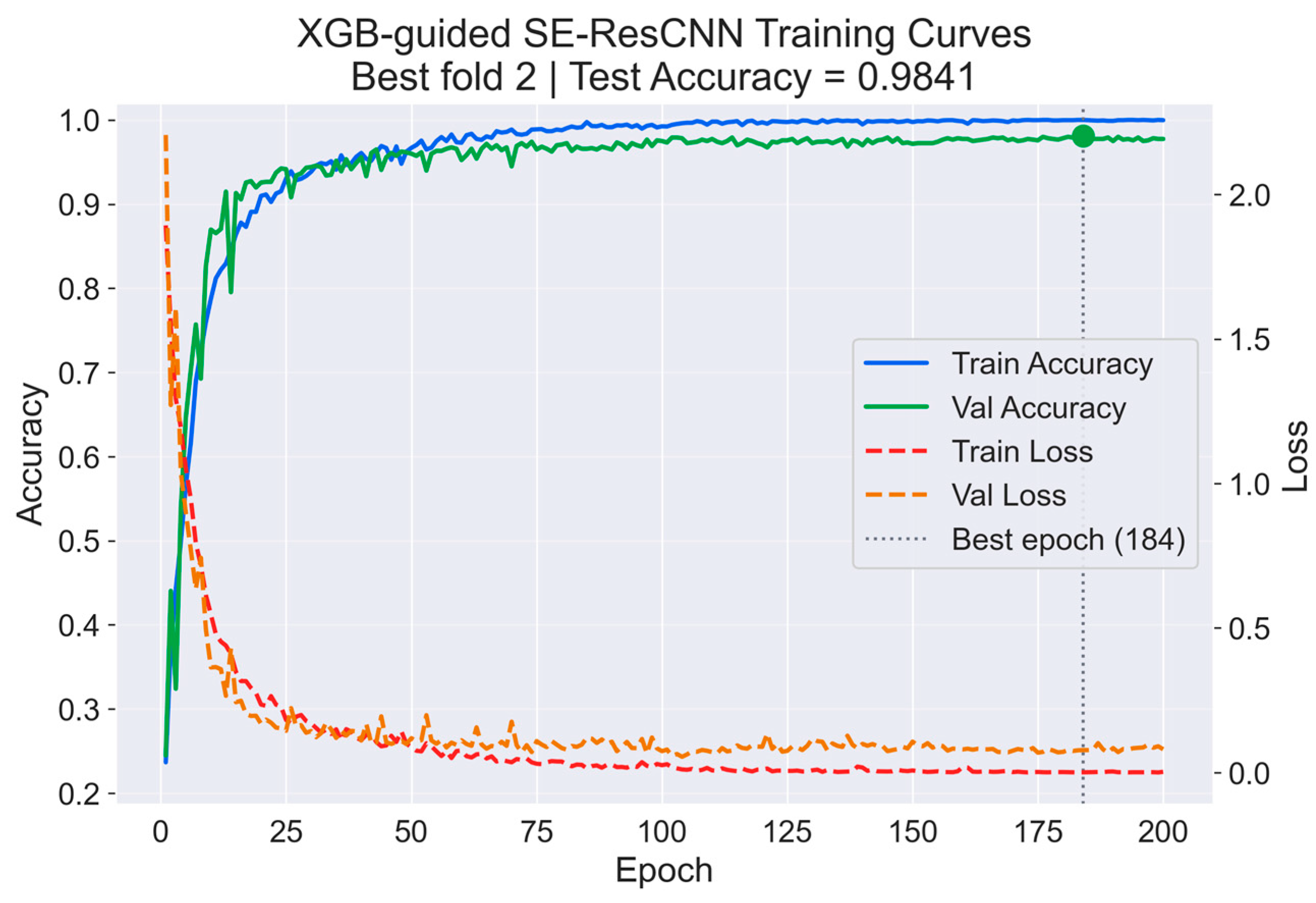
Figure 6 shows the training and validation accuracy and loss curves for the best-performing fold (Fold 2, test accuracy 98.41%). Both accuracy curves rise rapidly in the early training stage, with validation accuracy exceeding 0.90 within the first few tens of epochs and then remaining high with only mild fluctuations, while training accuracy continues to increase more gradually and approaches 1.00 in the later epochs. A small but persistent gap is visible between the training and validation accuracy curves, which is a common pattern in deep learning and generally indicates normal generalization behavior when the gap remains limited and stable. The loss curves show a similar convergence trend: both decrease sharply at the beginning, after which the training loss continues a slow downward decay while the validation loss stabilizes at a low but consistently higher level with minor oscillations. This suggests mild late-stage over-fitting, but without clear deterioration in validation performance.

Its practical impact is limited for two reasons. First, the model is retained at the epoch of highest validation accuracy rather than the final epoch; in Fold 2 this corresponds to epoch 184, with validation loss used as a tiebreak when validation accuracy is identical. Second, the architecture incorporates dropout in the classification head, which helps regularize training. Consistent with this, the validation accuracy remains close to its peak over a long range of epochs, and the test accuracy remains closely aligned with the best validation performance. Overall, the curve behavior indicates stable optimization and supports the conclusion that the checkpoint strategy successfully captures a well-generalizing model state despite the modest late-epoch train–validation gap.

For the analysis in the following sections, the eight class labels are briefly recalled here for clarity. Class 0 denotes gear pitting, Class 1 gear wear, Class 2 the healthy condition, Class 3 missing tooth, Class 4 compound tooth breakage with bearing inner-race fault, Class 5 compound tooth breakage with bearing outer-race fault, Class 6 gear tooth breakage, and Class 7 gear tooth crack. These fault categories were originally summarized in Table 2.

5.2. Classification Diagnostics

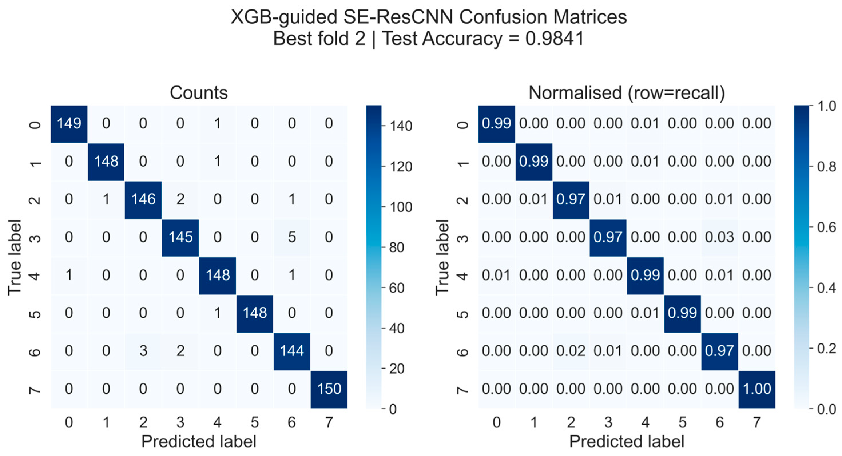
Figure 7 presents the confusion matrix for the best-performing fold (Fold 2, test accuracy of 98.41%), shown in both raw counts and row-normalized form.

The matrix reveals strong diagonal dominance across all eight gearbox condition classes, with per-class recall ranging from 0.97 to 1.00, confirming that the pipeline discriminates effectively across the full range of fault types under variable-speed operating conditions. Class 7 (gear tooth crack fault) achieves perfect recall, with all 150 test samples correctly classified. Classes 0 (gear pitting), 1 (gear wear), and 5 (compound outer-race fault) each attain a recall of approximately 0.99, with only a single sample misclassified in each case. Specifically, both Class 0 and Class 1 each produce one misclassification directed toward Class 4 (compound fault involving tooth breakage and bearing inner-race fault), while Class 5 misclassifies one sample as Class 4. Class 4 also achieves a recall of approximately 0.99, but with two misclassified samples rather than one: one sample is predicted as Class 0 and one as Class 6 (tooth breakage). These confusions are physically interpretable, as the compound fault classes include damage components that overlap with the spectral characteristics of individual gear-fault classes, making limited ambiguity between them mechanically plausible.

Classes 2 (healthy condition), 3 (missing-tooth fault), and 6 show slightly lower recall at about 0.97 and account for the most visible off-diagonal errors. Class 2 distributes four misclassified samples across three classes: one sample is predicted as Class 1, two as Class 3, and one as Class 6. This pattern suggests that a small number of healthy samples may contain weak transient or non-stationary vibration features that partially resemble fault-related responses, which is a recognized challenge in variable-speed gearbox diagnostics. Class 3 directs all five of its errors toward Class 6, indicating a concentrated confusion pathway rather than a broadly dispersed failure mode. Correspondingly, Class 6 misclassifies three samples as Class 2 and two as Class 3, forming a clear confusion relationship with Class 3 that is consistent with the shared characteristics of these damage mechanisms.

Overall, the confusion pattern is physically coherent and highly structured. Misclassifications are sparse and occur primarily between mechanically related classes, especially between gear-damage categories and compound faults that contain overlapping fault components, or between Classes 3 and 6, which both exhibit strong behavior associated with tooth damage. This structured misclassification pattern is further supported by the latent space analysis in Section 5.3. No evidence is seen of widespread random cross-class confusion. This indicates that the proposed pipeline has learned fault-relevant and physically meaningful representations rather than relying on arbitrary statistical correlations.

5.3. Latent Space Analysis

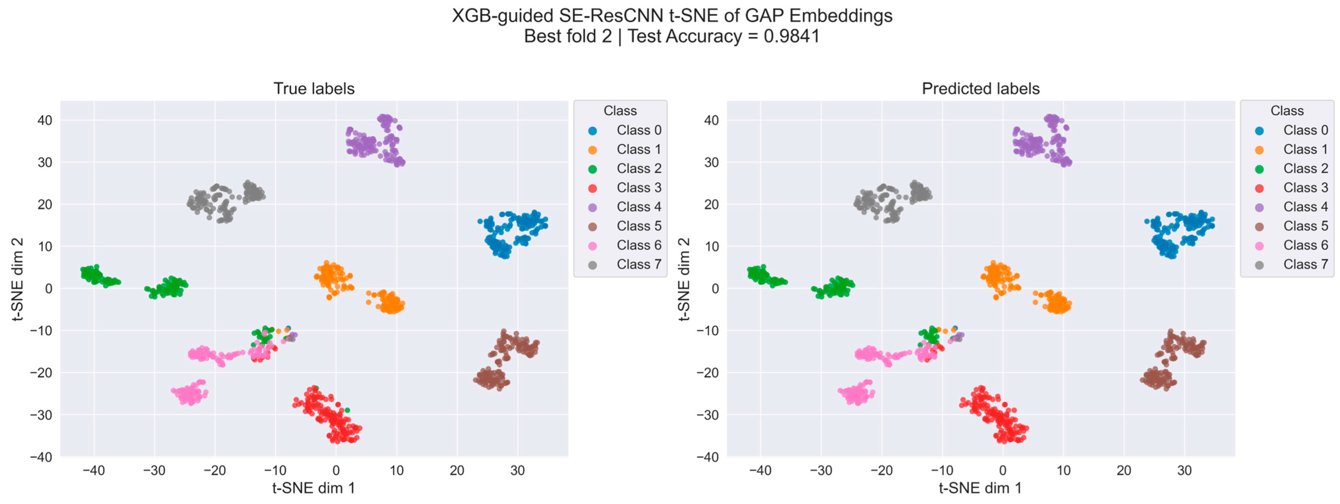
Figure 8 presents a two-dimensional t-SNE [46] projection of the 192-dimensional GAP embeddings extracted from the best-performing fold (Fold 2), computed for all 1197 test samples. The projection was generated using a perplexity of 40, 1000 optimization iterations, and PCA initialization. The two panels show the same embedding space colored by true labels (left) and predicted labels (right), which provide direct visual comparison between the latent class structure learned by the model and the final classification outcomes.

The visualization shows that the proposed pipeline learns a highly organized latent space, in which most classes occupy clearly separated regions with only limited local interaction. Class 0 (gear pitting), Class 4 (compound inner-race fault), Class 5 (compound outer-race fault), and Class 7 (gear tooth crack fault) are especially well isolated, each forming distinct cluster regions with no substantial visual mixing with unrelated classes. Class 1 (gear wear) and Class 2 (healthy condition) are also well separated overall, although both are distributed across more than one nearby local subcluster rather than forming a single compact group. This indicates that the learned representation is not only strongly class-discriminative, but also preserves meaningful within-class variation, which is consistent with the variable-speed operating conditions considered in this study.

The main area of reduced separation is located in the lower-central part of the embedding, where Class 3 (missing-tooth fault) and Class 6 (tooth breakage) lie in close proximity and show partial boundary overlap. This is the most prominent inter-class interaction visible in the figure and is fully consistent with the confusion pattern observed in Section 5.2, where the strongest misclassification pathway also occurred between these two classes. In addition, a small number of peripheral samples from other classes appear near this neighbor, particularly isolated points from Class 2 and Class 4. The local overlap is therefore not restricted to a perfectly clean two-class interface, but it is still dominated by the interaction between Class 3 and Class 6. Outside this region, the remaining classes retain clear geometric separation, with no evidence of widespread overlap across the latent space.

Comparing the two panels, the true-label and predicted-label views are highly consistent, with the predicted coloring following almost the same cluster arrangement as the ground-truth coloring. Differences between the panels are limited to a very small number of samples and are concentrated mainly around the boundary between Class 3 and Class 6, together with a few isolated points elsewhere. This close correspondence indicates that the classifier output is strongly aligned with the structure already present in the learned embedding space. The observed classification errors are therefore not associated with globally disordered or weakly separated representations but are concentrated within a small region of local overlap involving mechanically similar fault patterns.

From a mechanical perspective, the main overlap between Class 3 and Class 6 is reasonable, since both missing tooth and tooth breakage faults are forms of localized tooth damage. These faults can disrupt gear meshing, alter local mesh stiffness, and produce impact-type vibration responses, resulting in similar time–frequency patterns. The nearby Class 4 samples are also understandable because this compound class includes tooth breakage and thus shares gear-related characteristics with Class 6. The few Class 2 samples located in this region may be linked to weak transient responses or vibration variations caused by changing operating conditions under unsteady rotational speed. Therefore, the prominent overlap between Class 3 and Class 6, along with the nearby Class 4 and Class 2 samples, reflects physically meaningful similarities rather than random disorder in the embedding space.

Overall, the t-SNE projection provides further evidence that the XGB-guided SE-ResCNN pipeline learns fault-discriminative and physically meaningful representations. Most fault categories are mapped to clearly separated regions, while the remaining errors are confined to the most structurally similar conditions. This behavior is consistent with the confusion matrix analysis and supports the conclusion that the proposed method captures underlying fault-relevant structure rather than relying on incidental statistical correlations.

5.4. XGBoost Hard Selection Interpretation

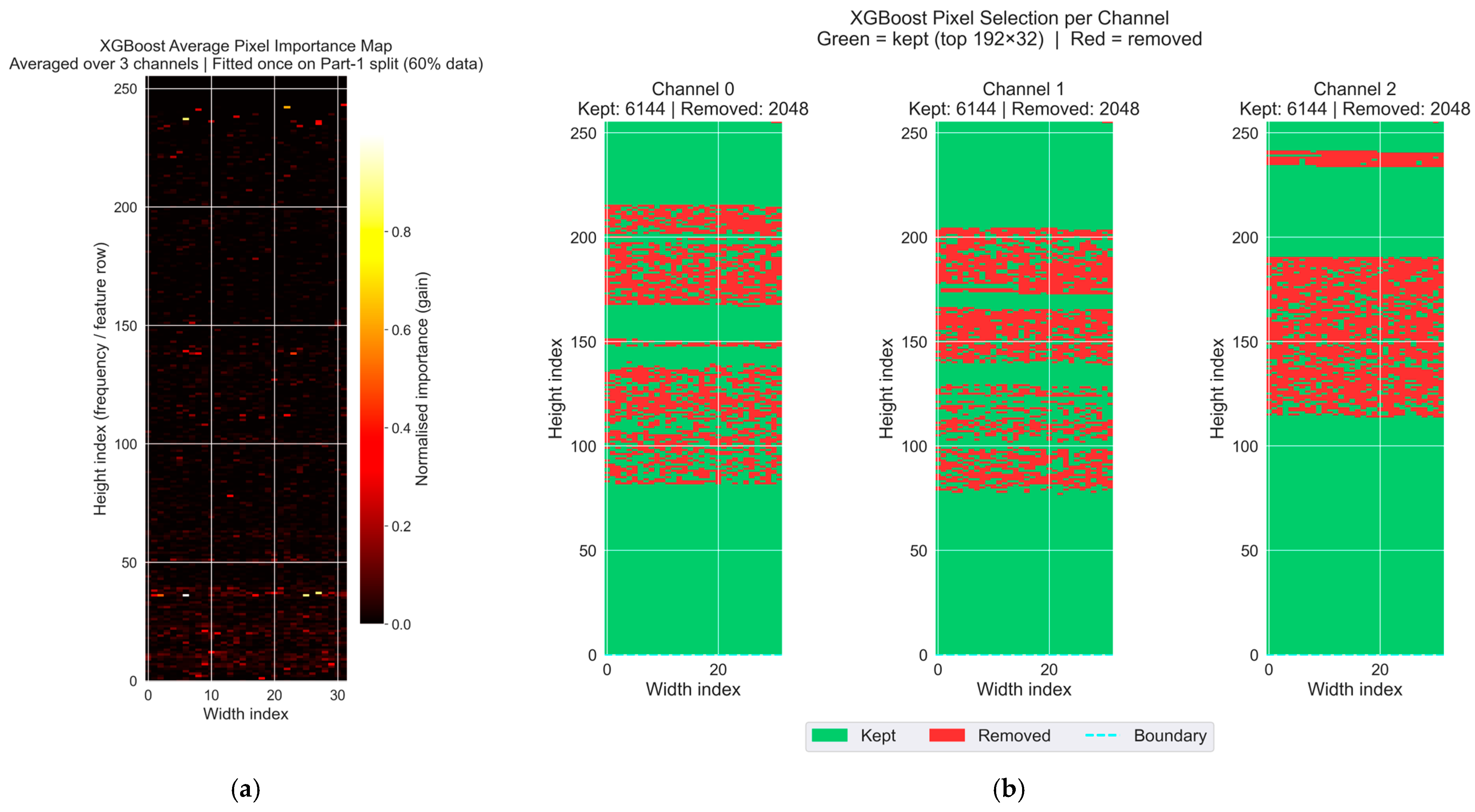
Figure 9 provides a direct interpretation of the hard selection performed in Stage 1. Figure 9a shows the average pixel importance map after averaging across the three channels, while Figure 9b shows the retained and removed pixels for each individual channel. Because the selector operates directly on the original time–frequency representation, these figures make it possible to interpret the hard selection behavior of Stage 1 and examine how the retained regions relate to physically meaningful characteristics in the spectrogram.

The average importance map in Figure 9a shows that informative pixels are not distributed evenly across the 256 × 32 time–frequency plane. Instead, the dominant pattern is selective concentration: high-importance regions appear as localized hotspots, while large areas remain weakly weighted. At a broader level, the map suggests that the low-frequency region contributes strongly overall, that parts of the middle-frequency region are comparatively less important, and that several high-frequency areas also carry notable discriminative information. This indicates that the classification decision depends on multiple separated time–frequency regions rather than on a single narrow band, with discriminative information distributed across several localized areas of the spectrogram.

The per-channel overlays in Figure 9b further clarify this behavior. Although the three channels show some structural similarities, their retained and removed pixel patterns are clearly different in detail. Channels 0 and 1 show more distributed removal patterns across several middle- to high-frequency regions, with removed pixels appearing in multiple separated horizontal bands. By contrast, Channel 2 contains larger continuous retained areas, while its removed pixels are more concentrated within a narrower middle-frequency region, together with a thin discarded strip near the upper end of the map. These differences indicate that XGBoost does not simply apply a uniform pruning rule across all input channels. Instead, the hard selection stage identifies the time–frequency locations that are most useful for classification within each individual channel. This supports the use of independent per-channel selection, as each vibration channel contains its own discriminative spectral structure, and the most class-relevant regions are not necessarily located at the same positions across channels.

Another clear pattern in Figure 9b is that many of the removed pixels are concentrated in horizontally extended bands. Since the vertical axis corresponds to frequency and the horizontal axis to time, this indicates that the hard selection is primarily frequency-oriented: XGBoost tends to suppress specific frequency ranges across multiple time positions, rather than removing isolated pixels at scattered locations. This suggests that, for the present task, the discriminative value of the STFT is governed more strongly by which frequency bands are retained than by highly localized time-position effects.

Overall, Figure 9 shows that the XGBoost stage performs a physically interpretable hard pruning of the STFT input. By suppressing less informative regions before deep feature extraction, Stage 1 reduces each channel from 256 × 32 to 192 × 32, lowering downstream computational cost while preserving the most diagnostically relevant information.

5.5. SE Block Channel Attention Analysis

This part examines the soft emphasis mechanism introduced by the SE block in Stage 2. Whereas Stage 1 uses XGBoost to perform hard selection directly on the STFT input, the SE block operates after convolutional feature extraction and re-weights the latent feature channels before classification. The purpose of this analysis is therefore to understand how the network modulates its deep representation after the input has already been pruned in the time–frequency domain.

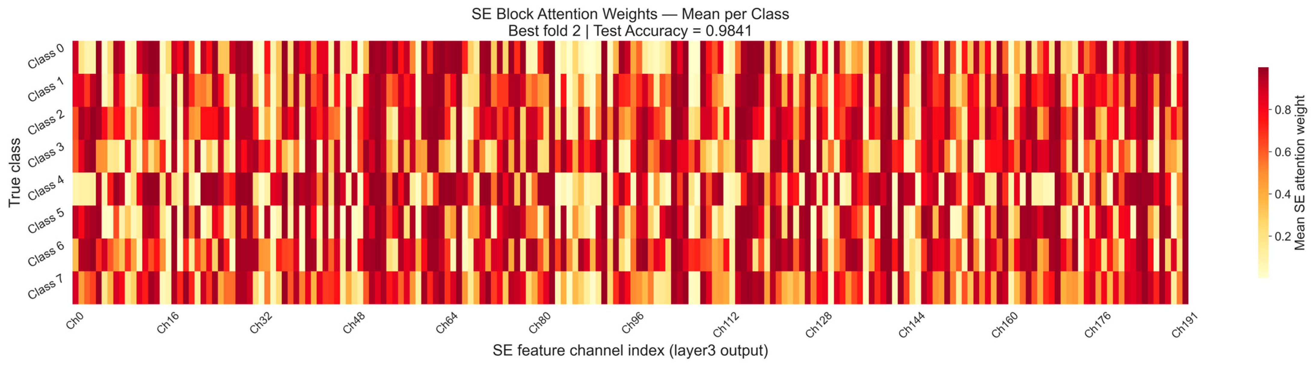
Figure 10 shows the mean SE attention weights for the 192 latent channels after Layer 3, averaged separately for each true class in the best-performing fold. Rather than being uniformly distributed across the channel dimension, the weights form a structured pattern with both shared and class-dependent components. Several channels remain strongly weighted across most classes, indicating that they capture broadly useful latent features that support representation of multiple fault conditions. In contrast, other channels show more visible changes across classes, suggesting that the SE block adjusts the relative emphasis of specific latent responses according to fault type. This distinction is important for interpretation: a channel with a consistently high average weight should be viewed as generally important to the learned representation, whereas class discrimination is more closely related to how the weighting of a channel varies across classes.

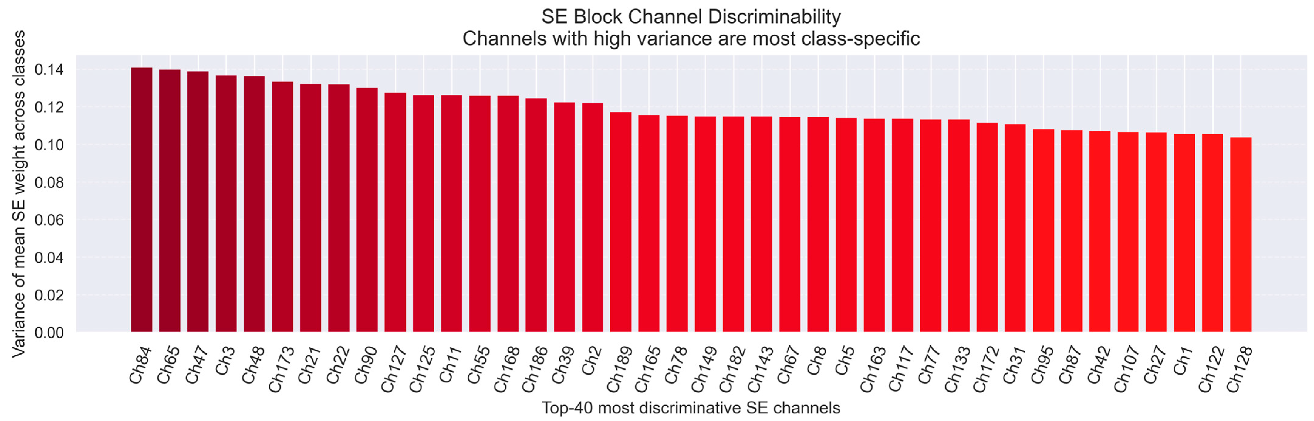
This distinction is clarified by Figure 11, which ranks the top 40 channels according to the variance of their mean SE weights across classes. Here, the focus is not on absolute weight magnitude, but on how strongly each channel’s weighting changes from one class to another. Channels with high variance are therefore the most class-sensitive channels, because their contribution is modulated more differently across fault categories. Conversely, channels that appear strongly weighted in Figure 10 but do not rank highly in Figure 11 are better interpreted as general-purpose channels that support the learned representation across many classes. Figure 11 thus complements the heatmap by identifying the subset of latent channels that exhibit the strongest class-dependent behavior.

Taken together, Figure 10 and Figure 11 show that the SE block performs a meaningful form of soft selection in the latent space. Some channels are emphasized consistently across classes, suggesting a more general representational role, while others are modulated more selectively and therefore contribute more strongly to inter-class differentiation. This behavior is structurally different from the XGBoost-based hard selection in Stage 1. XGBoost acts on the original STFT pixels and removes less informative input regions before feature extraction, whereas the SE block acts on learned feature channels and adaptively re-weights them after convolutional encoding. The two mechanisms therefore operate in different domains and serve complementary purposes, i.e., one reduces redundancy at the signal level, and the other refines class-relevant emphasis in the latent feature space.

5.6. Ablation

This subsection presents an ablation study to assess the contribution of each major design choice in the proposed framework. Specifically, the study examines the effect of using the original STFT map directly, adopting different map reduction strategies, and inserting different attention mechanisms into the Stage-2 residual classifier. The ablation is designed to answer the following three questions:

• Whether streamlining the STFT map can preserve classification performance while lowering the input size;
• Whether the XGBoost-based hard selection stage is more effective than learned reduction alternatives; and
• Whether additional attention further enhances the reduced representation.

For clarity of presentation, the compared variants are denoted as Methods 1–10, and their configurations are summarized in

Table 7. Definition of the compared methods used in the ablation study.

Method	Abbreviation	Description
1	Orig + CNN	Original STFT map with CNN
2	Orig + ResCNN	Original STFT map with ResCNN
3	TransSel + ResCNN	Transformer hard reduction followed by ResCNN
4	CNNSel + ResCNN	CNN scoring hard reduction followed by ResCNN
5	XGB + ResCNN	XGBoost-based hard reduction followed by ResCNN
6	XGB + TransSel + ResCNN	XGBoost hard reduction, soft Transformer selector, and ResCNN
7	XGB + SE (L1) + ResCNN	XGBoost hard reduction with SE after Layer 1 in ResCNN
8	XGB + CBAM + ResCNN	XGBoost hard reduction with CBAM and ResCNN
9	XGB + CBAM (Ch) + ResCNN	XGBoost hard reduction with channel-only CBAM and ResCNN
10	XGB + SE (L3) + ResCNN	XGBoost hard reduction with SE after Layer 3 in ResCNN

. To account for performance variation across random seeds while reducing the computational cost, the CV procedure used in the main experiment was removed. Instead, all methods were evaluated using four random seeds under a common fixed 60/20/20 train/validation/test split. This split was chosen to match the effective data allocation used in each fold of the CV setting, so that the same proportion of data was used for training, validation, and testing. In addition, the number of training epochs was reduced to 100, while training-related settings, such as batch size, learning rate, and weight decay, were kept unchanged. To ensure a fair comparison, for the models containing a Stage-1 map reduction block or a Stage-2 classifier block, the corresponding design and configuration were retained within the relevant comparison groups, so that the observed differences can be attributed mainly to the examined reduction or attention design rather than to unrelated changes in model structure or training setup.

Table 8. Quantitative results of the ablation study.

Method	Parameters	Mean Test Accuracy	Accuracy Std	F1 Mean	F1 Std	Mean Train Time	FLOPs
1	0.08 M	0.8997	0.0074	0.8992	0.0074	368.4	0.62 G
2	1.61 M	0.9710	0.0049	0.9710	0.0050	1138.8	1.91 G
3	1.61 M	0.9415	0.0092	0.9416	0.0092	869.5	1.43 G
4	1.61 M	0.9572	0.0122	0.9572	0.0122	868.1	1.43 G
5	1.61 M	0.9735	0.0014	0.9736	0.0014	869.4	1.43 G
6	1.70 M	0.9737	0.0014	0.9737	0.0015	975.4	1.44 G
7	1.61 M	0.9741	0.0030	0.9742	0.0030	895.5	1.43 G
8	1.61 M	0.9672	0.0060	0.9673	0.0059	991.1	1.43 G
9	1.61 M	0.9616	0.0038	0.9619	0.0037	907.9	1.43 G
10	1.62 M	0.9779	0.0039	0.9779	0.0040	877.9	1.43 G

presents the quantitative results of the ablation study. Methods 1 and 2 serve as full-input baselines, using the original 256 × 32 STFT maps without any map reduction. Replacing the shallow CNN in Method 1 with the ResCNN backbone in Method 2 improves the mean test accuracy from 89.97% ± 0.74% to 97.10% ± 0.49%, showing that the residual classifier provides a much stronger baseline on the original input. This also justifies the use of ResCNN as the common Stage-2 classifier in the later comparisons. Methods 3 to 5 then examine whether the input map can be reduced from 256 × 32 to 192 × 32 while maintaining classification performance. Among these three variants, Method 5 achieves the best result, with a mean test accuracy of 97.35% ± 0.14%, outperforming both Method 3 (94.15% ± 0.92%) and Method 4 (95.72% ± 1.22%), and slightly exceeding the full-input ResCNN baseline in Method 2 (97.10% ± 0.49%). This indicates that the XGBoost-based hard reduction strategy is more effective than the learned hard-reduction alternatives considered here, and that reducing the STFT map size can preserve, and in this case slightly improve, classification performance while lowering the input dimensionality.

Methods 6 to 10 were included to examine how different attention mechanisms interact with the XGBoost-reduced representation under the same Stage-2 classifier. In this group, Method 6 applies a soft Transformer-based re-weighting strategy, Methods 7 and 10 apply SE-based channel recalibration, and Methods 8 and 9 examine CBAM-based recalibration. The results show that these attention designs do not affect the reduced representation in the same way. Method 6 reaches a mean test accuracy of 97.37% ± 0.14%, very similar to the mean test accuracy of Method 5 (97.35% ± 0.14%), suggesting that an additional soft Transformer re-weighting stage does not provide clear benefit after the XGBoost-based hard reduction. Method 7, which inserts the SE block after Layer 1, achieves 97.41% ± 0.30%, only slightly exceeding the XGBoost-only baseline. This indicates that applying channel-wise recalibration at an early stage of the CNN provides limited additional improvement. Method 10, which inserts the SE block after Layer 3, achieves the highest mean test accuracy of 97.79% ± 0.39%. This result suggests that channel-wise recalibration is more beneficial when applied to the deepest CNN layer, where the feature channels contain more abstract and class-relevant representations. By contrast, Method 8 (96.72% ± 0.60%) and Method 9 (96.16% ± 0.38%) show that the CBAM-based variants are less effective in the present setting. This difference may be related to the already-pruned input representation. In Method 6, XGBoost has already removed many less informative time–frequency pixels before the Transformer selector is applied, so the additional soft re-weighting may increase complexity without adding substantial new discriminative information. A similar explanation applies to the CBAM variants. Given the compact feature set produced by the preceding XGBoost selection stage, the spatial attention component in CBAM may introduce redundant feature refinement or alter informative patterns that have already been effectively filtered by the preceding selection stage. In contrast, SE provides a simpler channel-wise recalibration mechanism that appears more compatible with the compact XGBoost-reduced representation. Overall, these observations indicate that, for the streamlined STFT maps considered here, deep-stage channel-wise recalibration provides the strongest observed performance among the tested attention configurations, with the deeper insertion producing a more noticeable benefit than early-stage recalibration.

In addition to the accuracy-based comparison, an efficiency-oriented analysis was conducted using classifier training time as the primary indicator, with parameter count and classifier Floating Point Operations (FLOPs) reported as complementary evidence. Here, the reported training time refers to the training time of the final neural classifier. The XGBoost-based hard selection stage was not included because it was used only once to construct the reduced STFT maps before classifier training and was not part of the iterative optimization process of the proposed model. Including this one-off preprocessing step in the same time measure would mix offline representation construction with the repeated training cost of the learnable classifier, thereby making the efficiency comparison less interpretable. The comparison shown in Table 8 demonstrates that the proposed method achieves the highest mean test accuracy among all compared variants while maintaining a classifier training time, parameter count, and FLOPs comparable to those of the other reduced-map ResCNN-based methods. Compared with the ResCNN baseline using the original STFT map, the proposed method increases the mean test accuracy from 97.10% to 97.79% while reducing the classifier training time from 1138.8 s to 877.9 s (around 23%) and the FLOPs from 1.91 G to 1.43 G.

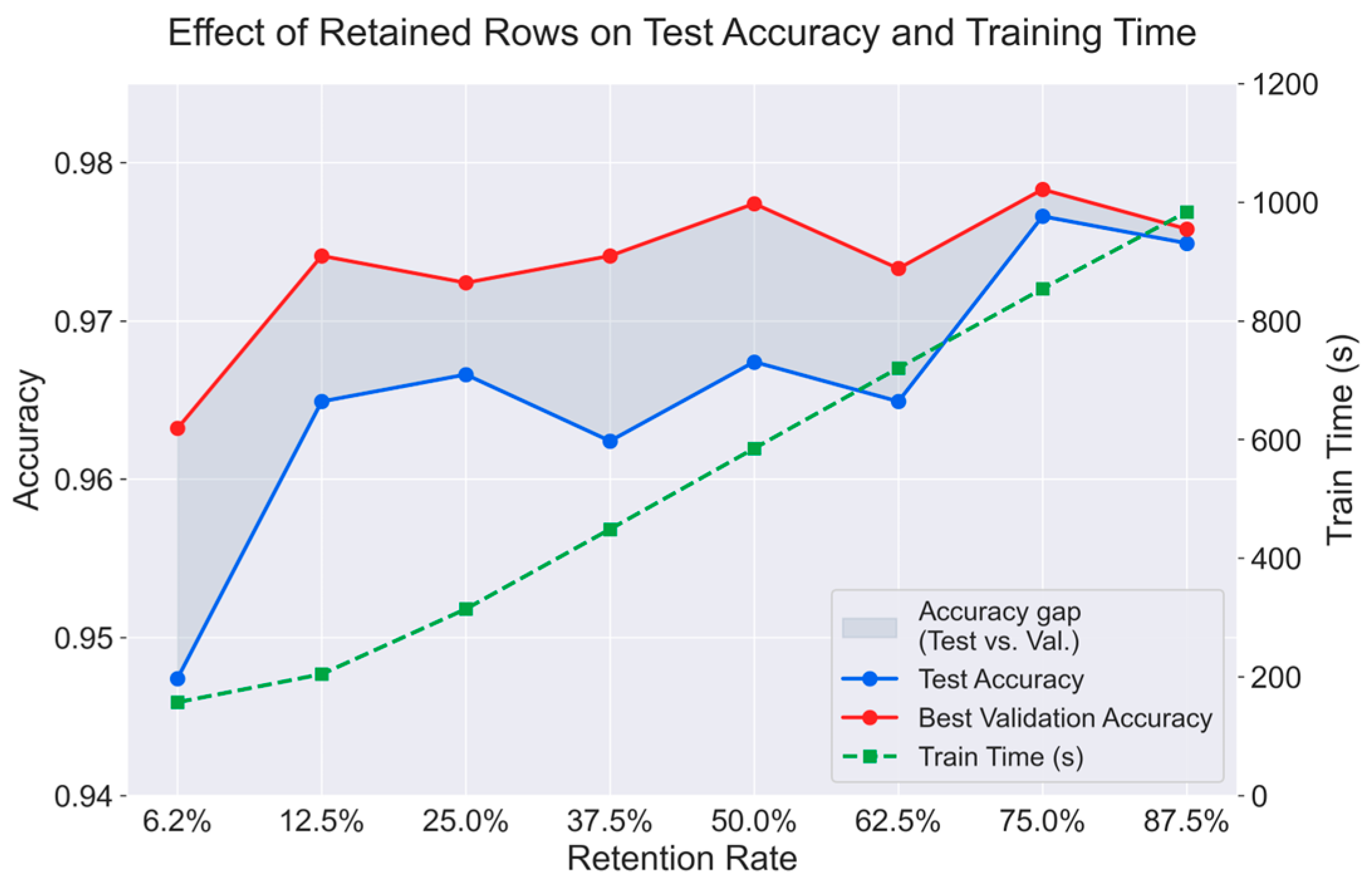
An additional study was conducted to examine the effect of the retained STFT map size within the proposed configuration. As shown in

Table 9. Study on the effect of retained STFT map size using the proposed method.

Test	Retained Rows	Retention Rate	Test Accuracy	Train Time	FLOPs	Best Validation	Epoch
1	224	87.5%	0.9749	983.4 s	1.67 G	0.9758	97
2	192	75%	0.9766	854 s	1.43 G	0.9783	96
3	160	62.5%	0.9649	720.4 s	1.20 G	0.9733	85
4	128	50%	0.9674	584.9 s	956.07 M	0.9774	99
5	96	37.5%	0.9624	448.8 s	717.07 M	0.9741	48
6	64	25%	0.9666	314.3 s	478.06 M	0.9724	97
7	32	12.5%	0.9649	204.5 s	239.06 M	0.9741	70
8	16	6.25%	0.9474	157.2 s	119.56 M	0.9632	47

, the variants with retention rates of 50% or above all maintain relatively high test accuracy, indicating that a moderate reduction of the spectrogram does not substantially damage the discriminative information required for classification. To further support the selection of the retained map size, Figure 12 visualizes the relationship among retention rate, test accuracy, best validation accuracy, and training time. As shown in Figure 12, reducing the retention rate generally decreases the classifier training time, but this efficiency gain does not always correspond to better diagnostic performance. Among the tested settings, the 75% retention rate (192 × 32) achieves the highest test accuracy while still reducing training time and FLOPs compared with the 87.5% setting and the full-input baseline. Although the 62.5% and 50% settings further reduce training time, both show lower test accuracy and a larger gap between best validation accuracy and test accuracy than the 75% setting, suggesting weaker generalization. Therefore, the 75% retention rate was selected as the best empirical trade-off in this study, balancing classification performance, generalization behavior, and computational efficiency.

Overall, the ablation study shows that the effectiveness of the proposed framework arises from the combination of XGBoost-based hard spectrogram reduction and deep-stage channel recalibration within the Stage-2 classifier. The comparison with the original-map baselines confirms that reducing the input map does not necessarily lead to a loss of discriminative information, while the comparison among different reduction and attention designs shows that the streamlined representation is most effectively refined by the SE mechanism applied at a deeper stage. The additional retained-map study further indicates that this design is not dependent on an arbitrary trimming level, but instead reflects a balance between information preservation and computational efficiency. Taken together, these results support the proposed configuration as a well-motivated design for achieving high classification performance with a compact input representation and reduced computational cost.

5.7. Sensitivity Analysis of Segmentation and XGBoost Selection Protocols

To further examine the influence of the segmentation strategy, an additional robustness experiment was conducted using non-overlapping vibration segments. In the main experiments, the signals were segmented using a window length of 2240 samples and a stride of 1024 samples. Although this setting increases the number of available samples, adjacent segments share part of the original raw signal. Therefore, when stratified random splitting is applied at the segment level, some test samples might be correlated with neighboring samples used during training. For the sensitivity experiment, the stride was set equal to the window length, while all other preprocessing settings, model architecture, training configuration, and evaluation procedures were kept unchanged. This reduced the total number of samples generated from 5984 to 2736. As shown in

Table 10. Segmentation sensitivity evaluation.

Metric	Stride = 2240 Data	Stride = 1024 Data
Accuracy	0.9503 ± 0.0096	0.9781 ± 0.0033
F1 Macro	0.9504 ± 0.0096	0.9782 ± 0.0033
Precision	0.9519 ± 0.0094	0.9785 ± 0.0032
Recall	0.9503 ± 0.0096	0.9781 ± 0.0033
Best Fold (Accuracy)	4 (0.9653)	2 (0.9841)
Total Samples	2736	5984

, the proposed method achieved a mean test accuracy of 95.03% ± 0.96%, with the best fold reaching 96.53% accuracy.

The lower accuracy under the non-overlapping setting should be interpreted together with the substantial reduction in data volume. Since the number of samples generated was reduced by more than half, the amount of data available for both XGBoost-based pixel selection and CNN training was also greatly decreased. This can directly affect the stability of the selected pixel mask and the generalization ability of the trained classifier. A repeated ablation check under the same non-overlapping setting using three random seeds showed the same qualitative pattern as the main ablation study, with the proposed configuration remaining among the best-performing reduced-input models. This indicates that using non-overlapping segmentation lowers the absolute accuracy but does not materially change the main experimental conclusion regarding the effectiveness of the proposed approach for variable-speed gearbox fault diagnosis.

In addition to the segmentation strategy, the influence of the XGBoost selection protocol was also examined. In the main evaluation, the XGBoost pixel selector was fitted once on a fixed 60% training partition, and the resulting pixel mask was reused across all cross-validation folds. This protocol is computationally efficient because XGBoost needs to be trained only once rather than independently in each fold. However, it also means that, in some folds, samples later used for testing may have contributed to the supervised estimation of the pixel-importance mask. Therefore, a nested selection experiment was conducted, in which XGBoost was re-fitted independently within each fold using only the corresponding fold-specific training partition before being applied to that fold’s validation and test sets. The original single-fit protocol achieved a mean accuracy of 97.81% ± 0.33%, while the nested protocol achieved 97.78% ± 0.28%. The difference of 0.03 percentage points is negligible and lies well within the inter-fold variation of either protocol, indicating that the two protocols produced practically equivalent performance in this study. Based on this result, the single-fit protocol was retained in the main experiments for computational efficiency. Nevertheless, the nested XGBoost selection protocol provides a stricter alternative and can be adopted when the additional computational cost of fitting XGBoost separately in each fold is acceptable.

6. Conclusions, Limitation, and Future Work

This paper proposed a two-stage hybrid framework for vibration-based wind turbine gearbox fault diagnosis. The first stage applies XGBoost directly to STFT spectrograms to identify and remove uninformative time–frequency pixels, reducing each channel from 256 × 32 to 192 × 32 while keeping the retained representation aligned with expert diagnostic reasoning. The second stage inserts an SE block after the deepest convolutional stage of a residual backbone, where it performs continuous channel-wise re-weighting on the learned feature maps. The two selectors operate on structurally different feature spaces and are complementary by design, i.e., one performs hard, discrete selection in the interpretable time–frequency domain, and the other performs soft, continuous emphasis in the abstract latent space. On an eight-class benchmark of approximately 6000 samples, the framework achieved a mean accuracy of 97.81% ± 0.33% under 5-fold stratified CV.

One limitation of this study is that the framework relies on having enough labeled data at both stages. Its performance has not yet been tested when labels are scarce, when classes are imbalanced, or in few-shot settings. These conditions are common in real industrial environments, and they are difficult for the framework because both stages need enough labeled examples to work well. To be specific, XGBoost needs them to rank pixel importance reliably, and the CNN needs them to learn useful features. Addressing this is a natural next step. Possible directions include pretraining the CNN backbone on unlabeled vibration data, adapting the XGBoost selector with class weights or cost-sensitive training, and exploring meta-learning, where the selected pixel mask is reused as a starting point across related fault types.