Operation Optimization of Direct Renewable-to-Load System Using Deep Reinforcement Learning

Abstract

Direct renewable-to-load systems have emerged as a promising pathway for improving local renewable energy utilization for large electricity consumers under constrained grid interaction and device operating limits. This paper investigates a park-level direct renewable-to-load system integrating battery energy storage and power-to-hydrogen facilities and formulates its operation problem as a sequential continuous-control task. A Deep Deterministic Policy Gradient (DDPG)-based scheduling framework is developed to explicitly model renewable generation, load demand, battery dynamics, hydrogen conversion and inventory evolution, renewable curtailment, storage-related operating cost, and the no-power-export operating boundary. Case studies based on measured wind/PV and load time-series data demonstrate that coordinated heterogeneous storage can effectively enhance system flexibility. Compared with single-type storage configurations, the coordinated battery–hydrogen scheme achieved the best overall storage performance, reducing the daily operating cost to CNY $25.28\times {10}^4$/day while increasing renewable energy utilization to 54.79%. Further benchmarking against MILP, GA, and a without-storage baseline shows that, although MILP remains the best offline benchmark, the proposed DDPG method provides a favorable trade-off between solution quality and online efficiency. Specifically, DDPG achieved an operating cost of CNY $20.93\times {10}^4$/day and a renewable energy utilization of 514.38 MWh, while requiring only 0.25 s/step for online inference. Typical-day analysis further reveals a clear functional complementarity between the two storage types; battery storage mainly provides fast short-term regulation, whereas the hydrogen subsystem mainly supports longer-duration energy shifting. These results indicate that the proposed framework offers a practical and efficient solution for the operation optimization of direct renewable-to-load systems under no-power-export constraints.

1. Introduction

The rapid growth of renewable energy deployment is reshaping modern power systems toward low-carbon and sustainable operation. In parallel, large electricity consumers such as industrial facilities and commercial parks are increasingly seeking direct access to renewable electricity to reduce carbon emissions, enhance energy autonomy, and stabilize long-term energy costs [1]. Recent studies have also shown that green transition and climate adaptation are closely related to corporate resilience and sustainable development in the low-carbon economy [2]. As a result, local renewable-powered supply schemes where renewable generation is preferentially utilized by nearby loads have attracted growing attention as an effective approach to improve local renewable utilization and reduce reliance on centralized grid dispatch [3].

In China, green electricity direct connection (direct renewable-to-load supply) has been formally promoted as an institutional mechanism to integrate renewable production and consumption. The national notice jointly issued by the National Development and Reform Commission (NDRC) and the National Energy Administration (NEA) defines green electricity direct connection as a system where renewable generation (e.g., wind, solar, biomass) supplies a single electricity user through dedicated lines without directly feeding into the public grid, enabling physically traceable green electricity consumption [4]. It further distinguishes grid-interactive and off-grid types, clarifies responsibility boundaries at the point of interconnection, and specifies typical source-load matching requirements. For grid-interactive projects, it requires the annual self-consumed renewable electricity to be no less than 60% of total available renewable generation and no less than 30% of total electricity consumption, with a directive to further increase the self-consumption ratio (e.g., at least 35% before 2030), and suggests an upper bound for export ratio generally not exceeding 20% (subject to provincial refinements) [5].

Driven by the national framework, regional deployments have quickly diversified across provinces. Notably, typical practices in Yunnan, Inner Mongolia, and Shandong highlight distinct industrial motivations, grid interaction rules, and flexibility configurations, which in turn impose different operational bottlenecks [6,7]. Yunnan leverages its strong clean-energy endowment to build full green electricity supply pathways for zero-carbon parks and has issued provincial-level implementation measures while advancing a first batch of projects. Inner Mongolia, featuring large-scale wind/solar resources and national computing hubs, has promoted data-center-oriented direct supply and released province-level rules emphasizing source-load matching and strict export constraints for most project types. Shandong, as a major industrial province with strong decarbonization pressure, has started off-grid-style 100% green electricity direct connection park-level projects using wind–solar coupling and grid-forming technologies to support high-reliability manufacturing loads. A comparative view of these representative practices is summarized in

Table 1. Representative regional practices and operational characteristics of direct renewable-to-load systems.

Region	Main Application	Grid Interaction	Export Rule	Flexibility Focus
Yunnan	Zero-carbon parks	Grid-interactive	Capped/conditional	BESS + flexible loads/VPP
Inner Mongolia	Data centers	Grid-interactive	Strict/conditional	Storage + load shaping
Shandong	Industrial parks	Near-off-grid/islanded	Prohibited	Grid-forming + storage

.

From an engineering perspective, these regional practices collectively imply a common technical core; the operation must simultaneously manage volatile variable renewable energy (VRE) and time-varying demand under practical operational constraints [8]. These constraints include interconnection capacity limits (for grid-interactive projects), strict restrictions on reverse power flow/export (for many project types), minimum self-consumption ratios for compliance and verification, and device-level operating constraints of storage and conversion units. When such constraints are binding, naïve dispatch may lead to excessive curtailment, increased purchase cost, or even infeasible operating points [9].

To further enhance flexibility and renewable utilization, energy storage technologies are increasingly integrated into direct renewable-to-load systems [10]. Battery energy storage systems (BESSs) provide fast short-term balancing and power regulation, whereas power-to-hydrogen technologies enable long-duration energy storage by converting surplus renewable electricity into chemical energy that can be stored and later converted back to electricity [11]. In practical deployments, the coordinated operation of renewable generation, battery storage, hydrogen production/storage/utilization, and load demand offers additional degrees of freedom but also introduces strong multi-timescale coupling and complex feasibility boundaries [12]. For example, batteries are well suited to mitigate minute-level fluctuations but can suffer from frequent cycling and throughput-based wear cost, while hydrogen systems feature slower dynamics and efficiency losses yet provide energy shifting over longer horizons [13].

A large body of literature has studied optimal operation and energy management of renewable-based power systems. Conventional approaches commonly employ mathematical programming and dynamic optimization techniques, such as mixed-integer linear programming (MILP) and dynamic programming, to obtain optimal scheduling decisions under known time-series information and well-defined system models [14]. In addition, meta-heuristic optimization algorithms have also been widely applied to microgrid energy management because of their flexibility in handling nonlinear and nonconvex scheduling problems. For example, Liu et al. proposed a DE-HHO hybrid meta-heuristic framework for microgrid energy management and demonstrated its effectiveness in reducing operating cost and improving optimization performance [15]. These optimization-based and meta-heuristic methods can achieve optimal or near-optimal solutions under given forecasts and explicit models, but they generally rely on repeated full-horizon or rolling re-optimization to respond to evolving operating states, which may limit their real-time applicability under time-varying renewable generation and load conditions [16]. Moreover, simplified representations of heterogeneous storage dynamics, conversion processes, and operational constraints may lead to infeasible schedules when grid-exchange limits become binding or renewable fluctuations exceed forecast ranges [17]. Such issues are increasingly exposed in direct renewable-to-load projects, where strict export rules and tight interconnection margins are frequently active constraints in practice [18].

In recent years, deep reinforcement learning (DRL) has emerged as a promising data-driven approach for sequential decision-making in complex energy systems [19]. Unlike model-based optimization, DRL can learn adaptive control policies through interaction with the environment and can handle high-dimensional state spaces and nonlinear dynamics. DRL has been applied to microgrid management, demand response, and renewable integration problems, showing advantages in sequential decision-making, nonlinear system control, and online response to time-varying operating conditions [20,21,22]. However, existing studies largely focus on generalized microgrid settings and often overlook the operational characteristics that are central to direct renewable-to-load systems: binding grid-exchange and export constraints, compliance-oriented minimum self-consumption requirements, and the multi-timescale coordination of heterogeneous storage (battery + hydrogen) under continuous control [23].

Motivated by the above gaps and regional practice implications, this paper studies a direct renewable-to-load system in which renewable generation is physically connected to a dedicated load through a dedicated park-level AC distribution corridor, including renewable collection feeders, step-up/down transformers, internal switchgear, metering devices, and a local distribution bus. This dedicated infrastructure is separated from the public grid except at the point of common coupling (PCC), where only grid import is allowed. The system incorporates BESS and power-to-hydrogen facilities to provide both short-term and long-term flexibility. The primary objective is to maximize local renewable utilization while minimizing operating cost under explicit constraints on grid exchange (when applicable), export restrictions, and device feasibility [24].

Existing approaches for renewable-powered supply operation can be broadly categorized into deterministic optimization-based methods, meta-heuristic optimization methods, and reinforcement-learning-based methods. For clarity,

Table 2. Summary of representative methods.

Method Category	Algorithm	Characteristics
Deterministic optimization-based	MILP	Global optimum under given forecasts; High computational burden
Meta-heuristic optimization	GA, DE-HHO [15]	Meta-heuristic search; Forecast-dependent
Reinforcement learning	DDPG	Off-policy actor–critic for continuous actions; Requires constraint-aware execution [26]

summarizes representative algorithms and their typical characteristics, highlighting the limitations that motivate the proposed framework [25].

To further clarify the differences among existing studies and identify the research gap addressed in this work, a more detailed comparison of the reviewed studies is provided in

Table 3. Summary of related studies on renewable-based energy management and storage scheduling.

Research Stream	Techniques/Algorithms Used	Typical Evaluation Metrics	Main Advantages	Main Limitations
Deterministic optimization	MILP, LP, DP, MPC	Cost, curtailment, constraint satisfaction, computation time	Explicit modeling of physical constraints; high solution quality under known forecasts	Forecast-dependent; computational burden increases with complex storage and grid constraints
Meta-heuristic optimization	GA, PSO, HHO, DE-HHO, evolutionary algorithms [15]	Objective value, convergence, cost, renewable utilization	Flexible for nonlinear and nonconvex problems; easy to implement	No guarantee of global optimality; sensitive to parameter settings
Reinforcement learning	Q-learning, DQN, DDPG, PPO, SAC	Reward, cost, renewable utilization, violation rate, inference time	Sequential decision-making under time-varying conditions; fast online execution after training	Training stability and constraint satisfaction require careful design
Direct renewable-to-load operation with heterogeneous storage	Source–load matching, battery–hydrogen scheduling, grid-constrained dispatch	Self-consumption, renewable utilization, curtailment, storage state, cost	Supports local renewable consumption and exploits complementary storage characteristics	Continuous-control scheduling under strict no-power-export constraints remains insufficiently studied

. The comparison focuses on the techniques or algorithms used, typical evaluation metrics, main advantages, and remaining limitations.

As summarized in Table 3, existing studies have provided valuable methods for renewable-based energy management and storage scheduling. However, limited attention has been paid to continuous-control operation of direct renewable-to-load systems under strict no-power-export constraints, especially when battery storage and hydrogen storage need to be coordinated within a unified sequential decision-making framework. This gap motivates the DDPG-based coordinated scheduling method developed in this paper.

To address these challenges, we formulated day-ahead/intra-day operation as a sequential continuous-control problem and developed a DRL-based scheduling framework implemented with the Deep Deterministic Policy Gradient (DDPG) algorithm [27]. The environment model explicitly represents the interactions among renewable supply, load demand, battery dynamics, hydrogen conversion and inventory evolution, and grid exchange. To enhance feasibility under binding constraints, actions generated by the agent are projected into the admissible operating region, and penalty terms are incorporated during training to discourage constraint violations. Case studies based on representative industrial-park scenarios demonstrate that the proposed approach can generate stable and executable schedules under time-varying renewable generation and load conditions, reduce operating cost and curtailment, and improve renewable utilization while respecting practical operational constraints [28].

The main contributions of this paper are summarized as follows. First, a direct renewable-to-load operation model is established for park-level electricity consumers under practical grid-interaction restrictions, in which the no-power-export boundary, renewable curtailment, battery dynamics, hydrogen conversion, and hydrogen inventory evolution are explicitly considered. Second, a DDPG-based continuous-control scheduling framework is developed to coordinate battery energy storage and hydrogen energy storage with different regulation characteristics, enabling the system to exploit both short-term power regulation and longer-duration energy shifting. Third, comprehensive case studies are conducted using measured wind/PV and load time-series data, and the proposed method is compared with MILP, GA, and a without-storage baseline to evaluate its operational economy, renewable energy utilization, and online decision-making efficiency.

2. System Modeling of the Direct Renewable-to-Load System

2.1. System Description and Configuration

This study considers a direct renewable-to-load supply system in which renewable generation facilities are physically connected to specific electricity consumers through dedicated infrastructure. The primary objective of the system is to maximize local utilization of renewable energy while maintaining reliable power supply and satisfying operational constraints. Unlike conventional grid-connected renewable energy systems, the proposed configuration prioritizes direct consumption of locally generated renewable electricity, while grid power is mainly used as supplementary support when local generation is insufficient. 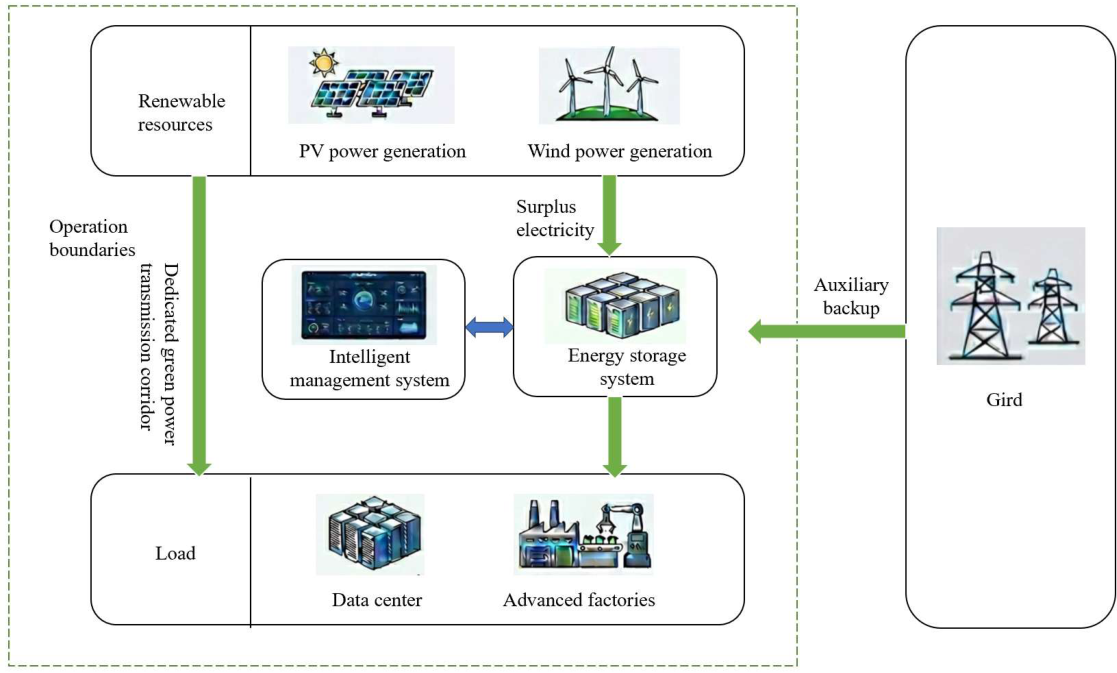Figure 1 illustrates the system boundary and the PCC-based grid interaction of the direct renewable-to-load supply system.

As illustrated in Figure 1, the direct renewable power supply system is configured within a clearly defined operational boundary, encompassing renewable resources, an intelligent management system (IMS), an energy storage system, and local loads. On the source side, photovoltaic (PV) and wind power generation constitute the primary renewable supply, while the load side comprises representative high-energy consumers such as data centers and advanced factories. Within this framework, a dedicated green power transmission corridor ensures the direct and preferential delivery of renewable electricity to the load. Concurrently, surplus electricity generated by the renewable sources is routed to the energy storage system, which dynamically interacts with the IMS for coordinated operation. Finally, the external utility grid is integrated as an auxiliary backup, providing supplementary support to guarantee the overall power supply reliability when local resources are insufficient.

In this study, the term “dedicated infrastructure” refers to the private park-level electrical connection that links the renewable generation side and the local load side. It includes renewable collection lines, transformers, internal AC distribution feeders, switchgear, metering devices, and the local distribution bus within the park boundary. The battery energy storage system and the power-to-hydrogen subsystem are connected to this internal distribution bus and are coordinated by the intelligent management system. The public utility grid is connected only through the PCC and is used as an auxiliary power source when local renewable generation and storage discharge cannot fully meet the load demand. Since power export is prohibited in the considered operating mode, reverse power flow from the park system to the public grid is not allowed. The internal dedicated infrastructure is modeled as an aggregated energy-transfer path, and detailed network power-flow constraints, voltage constraints, and line losses inside the park are not explicitly considered in this paper.

At each time step, system operation must maintain power balance among renewable generation, load demand, storage charging/discharging, hydrogen production or consumption, grid support, and renewable curtailment. The integration of heterogeneous storage technologies introduces strong multi-timescale coupling between instantaneous power regulation and longer-term energy state evolution, which significantly increases the complexity of coordinated scheduling.

Based on the system configuration illustrated in Figure 1, a quantitative representation of power exchange and energy balance is required to support subsequent optimization and control design. In particular, the interactions among renewable generation, load demand, storage operation, hydrogen conversion processes, metering and dispatch functions, and auxiliary grid support should be explicitly modeled within a unified framework. The mathematical formulation of power balance and operational constraints for the direct renewable-to-load system is discussed in the following section.

2.2. Operation Requirements

Before formulating the detailed operational constraints, the boundary conditions and operating limits adopted in the model are summarized to clarify the feasible operating region of the direct renewable-to-load system. The system boundary is defined at the park-level direct renewable-to-load interface, including wind/PV generation, local load, battery energy storage, the power-to-hydrogen subsystem, and the PCC-based interaction with the utility grid. The utility grid is used only as an auxiliary power source, and power export to the public grid is prohibited in this study. The operation horizon is discretized into 15 min intervals over a 24 h scheduling period. Renewable generation can either be absorbed by the local load, stored by the battery, consumed by the electrolyzer, or curtailed when it exceeds the admissible absorption capability. The battery and hydrogen subsystems are constrained by their rated power limits, state boundaries, and conversion efficiencies. These boundary conditions are summarized in

Table 4. Boundary conditions and operating limits used in the model development.

Boundary Category	Boundary Condition
Grid interaction boundary	$P_{\mathrm{grid} }^{\min }\le { P}_{\mathrm{grid}}(t) \le { P}_{\mathrm{grid}}^{\max }$
No-power-export boundary	${ P}_{\mathrm{grid}}(t)$ ≥ 0
Battery power boundary	$0 \le P_{\mathrm{bat}}^{\mathrm{ch}}(t) \le {u_{\mathrm{b}\mathrm{a}t}(t)P}_{\mathrm{bat},\mathrm{ch}}^{\max }$ $0 \le P_{\mathrm{bat}}^{\mathrm{dis}}(t) \le (1-u_{\mathrm{b}\mathrm{a}t}(t))P_{\mathrm{bat},\mathrm{dis}}^{\max }$ $u_{\mathrm{b}\mathrm{a}t}(t)$ ∈ {0, 1}
Battery SOC boundary	${\mathit{SOC}}_{\min } \le \mathit{SOC}(t) \le {\mathit{SOC}}_{\max }$
Hydrogen conversion boundary	$0 \le { P}_{\mathrm{ele}}(t) \le {u_{{ \mathrm{H}}_2}(t)P}_{\mathrm{ele}}^{\max }$ $0 \le { P}_{\mathrm{fc}}(t) \le { (1-u_{{ \mathrm{H}}_2}(t)) P}_{\mathrm{fc}}^{\max }$ $u_{{ \mathrm{H}}_2}(t)$ ∈ {0, 1}
Hydrogen storage boundary	$H_2^{\min } \le { H}_2(t) \le { H}_2^{\max }$

.

2.2.1. Power Balance Constraints

The operation of a direct renewable-to-load system is governed by the instantaneous balance between energy supply and demand. At each time step, the electricity generated from renewable sources, together with grid support and energy storage operation, must satisfy local load demand as well as the power consumption of the hydrogen production system, while accounting for possible renewable curtailment. A mathematical representation of this balance is essential for subsequent optimization and control design.

Let $P_{\mathrm{w}}(t)$ and $P_{\mathrm{pv}}(t)$ denote the actual absorbed wind power and actual absorbed photovoltaic power of the system respectively at time step $t$, $P_{\mathrm{load}}(t)$ the local electricity demand, $P_{\mathrm{grid}}(t)$ the power exchanged with the utility grid (positive for import and negative for export), ${ P}_{\mathrm{bat}}^{\mathrm{ch}}(t)$ and ${ P}_{\mathrm{bat}}^{\mathrm{dis}}(t)$ the charging and discharging power of the energy storage system, respectively, ${ P}_{\mathrm{ele}}(t)$ the electricity consumed by the electrolyzer for hydrogen production, and $P_{\mathrm{fc}}(t)$ the output power of the fuel cell. The instantaneous power balance can be expressed as follows:

$$P_{\mathrm{w}}(t) +{ P}_{\mathrm{pv}}(t) + P_{\mathrm{grid}}(t) +{ P}_{\mathrm{bat}}^{\mathrm{dis}}(t) + P_{\mathrm{fc}}(t) = P_{\mathrm{load}}(t) +{ P}_{\mathrm{bat}}^{\mathrm{ch}}(t) +{ P}_{\mathrm{ele}}(t)$$

(1)

This equation ensures that all electricity flows within the system are properly accounted for, including renewable utilization, storage operation, grid interaction, and hydrogen production demand. Renewable generation exceeding the sum of local consumption, storage charging capacity, hydrogen production capacity, and allowable export limits must be curtailed.

In practical operation, the renewable generation term represents the actual absorbed wind and solar resources, reflecting their intermittent and uncertain nature. The grid exchange term provides supplementary supply when local generation is insufficient and may also enable limited export of surplus electricity depending on interconnection policies. Energy storage acts as a buffer that shifts energy across time, while the hydrogen production system provides an additional flexible load that can absorb surplus renewable energy and enhance local utilization.

2.2.2. Grid Interaction Constraints

The national policy framework for green electricity direct connection clarifies the physical/responsibility boundary at the PCC and imposes restrictions on reverse power flow. In regions where the electricity spot market is not continuously operated, grid-interactive projects are not allowed to export power to the public grid. When export is permitted, the exported energy is generally capped (e.g., the export ratio is usually limited to no more than 20% of the available renewable generation, subject to provincial implementation). The power exchanged between the local system and the utility grid is limited by the interconnection rating at the point of common coupling (PCC) and by regulatory requirements for direct renewable-to-load projects. Therefore, the grid exchange power is constrained as follows:

$$P_{\mathrm{grid} }^{\min }\le { P}_{\mathrm{grid}}(t) \le { P}_{\mathrm{grid}}^{\max }$$

(2)

where $P_{\mathrm{grid} }^{\min }$ and ${ P}_{\mathrm{grid}}^{\max }$ denote the minimum and maximum allowable grid exchange capacity. Positive values represent power import, while negative values represent export. In the present study, power export to the public grid is prohibited. Therefore, the lower bound of grid exchange is set to zero, and the system is allowed to import electricity from the grid only within the admissible PCC capacity.

It should be noted that this zero-export setting is adopted as a conservative strict operating boundary for the case study, rather than as a universal representation of all PCC agreements. In practical projects, a small amount of momentary reverse power flow may be tolerated depending on the interconnection contract, protection settings, metering rules, and provincial implementation requirements. Such cases can be represented by relaxing the lower bound of ${ P}_{\mathrm{grid}}(t)$ according to the allowable export tolerance. However, the present study focuses on the strict no-power-export scenario because it imposes a more restrictive condition on local renewable absorption and storage coordination. Under this setting, surplus renewable generation must be consumed locally, stored by the battery or hydrogen subsystem, or curtailed, which provides a conservative test of the proposed scheduling method under tight grid-interaction constraints.

2.2.3. Energy Storage Constraints

Energy storage devices provide essential flexibility for balancing renewable generation fluctuations and load variations in the direct renewable-to-load system. In this study, both the electrochemical battery storage system and the hydrogen storage subsystem are modeled explicitly. Their operation is constrained by rated power limits, energy state evolution, and feasible operating modes. Incorporating these constraints is necessary to ensure that the scheduling strategy remains physically meaningful and practically implementable.

For the battery energy storage system, the charging and discharging power are limited by the converter rating, and the state of charge is updated according to the charging/discharging process. The corresponding operational constraints are given as follows:

$$0 \le P_{\mathrm{bat}}^{\mathrm{ch}}(t) \le P_{\mathrm{bat},\mathrm{ch}}^{\max }, 0 \le P_{\mathrm{bat}}^{\mathrm{dis}}(t) \le P_{\mathrm{bat},\mathrm{dis}}^{\max }$$

(3)

$$E_{\mathrm{bat}}(t+1)=E_{\mathrm{bat}}(t)+{\eta }_{\mathrm{ch}}{P}_{\mathrm{bat}}^{\mathrm{ch}}(t)\Delta t - {\displaystyle \frac{1}{{\eta }_{\mathrm{dis}}}}{P}_{\mathrm{bat}}^{\mathrm{dis}}(t)\Delta t$$

(4)

$$\mathit{SOC}(t)={\displaystyle \frac{E_{\mathrm{bat}}(t)}{E_{\mathrm{bat}}^{\mathrm{cap}}}}$$

(5)

$${\mathit{SOC}}_{\min } \le \mathit{SOC}(t) \le {\mathit{SOC}}_{\max }$$

(6)

where $E_{\mathrm{bat}}^{\mathrm{cap}}$ is the storage energy capacity, and ${ \eta }_{\mathrm{ch}}$ and ${\eta }_{\mathrm{dis}}$ are the charging and discharging efficiencies. Moreover, simultaneous charging and discharging are physically prohibited. Therefore, a binary variable $u_{\mathrm{b}\mathrm{a}\mathrm{t}}(t)$ is introduced. Accordingly, the mutual exclusiveness is represented by the following:

$$0 \le P_{\mathrm{bat}}^{\mathrm{ch}}(t) \le {u_{\mathrm{b}\mathrm{a}\mathrm{t}}(t)P}_{\mathrm{bat},\mathrm{ch}}^{\max }$$

(7)

$$0 \le P_{\mathrm{bat}}^{\mathrm{dis}}(t) \le (1-u_{\mathrm{b}\mathrm{a}\mathrm{t}}(t))P_{\mathrm{bat},\mathrm{dis}}^{\max }$$

(8)

$$u_{\mathrm{b}\mathrm{a}\mathrm{t}}(t)\in \{0,1\}$$

(9)

where $u_{\mathrm{b}\mathrm{a}\mathrm{t}}(t)$ denotes the battery operating status. This treatment preserves physical feasibility while maintaining a mixed-integer linear formulation.

In addition to electrochemical storage, the hydrogen storage subsystem provides longer-duration flexibility through electricity-to-hydrogen conversion, hydrogen storage, and hydrogen-to-electricity reconversion. A hydrogen energy storage system consists of an electrolyzer, a hydrogen tank, and a fuel cell. The model is given as follows.

• Electrolyzer: The electrolyzer converts electrical energy into hydrogen energy. The hydrogen production rate is proportional to the input power, considering the electrolyzer efficiency ${\eta }_{ele}$:

$$m_{{\mathrm{H}}_2}^{\mathrm{prod}}(t) = {\displaystyle \frac{{\eta }_{\mathrm{ele}} P_{\mathrm{ele}}(t) \Delta t}{H_{\mathrm{HV}}}}$$

(10)

where $H_{\mathrm{H}\mathrm{V}}$ denotes the higher heating value of hydrogen, and $m_{{\mathrm{H}}_2}^{\mathrm{p}\mathrm{r}\mathrm{o}\mathrm{d}}$ is the hydrogen production.

• Hydrogen Tank: The hydrogen mass balance is expressed as follows:

$$m_{{\mathrm{H}}_2}(t+1)=m_{{\mathrm{H}}_2}(t)+{ m}_{{\mathrm{H}}_2}^{\mathrm{prod}}(t)-m_{{\mathrm{H}}_2}^{\mathrm{cons}}(t)$$

(11)

where $m_{H_2}^{cons}(t)$ is the hydrogen consumption. Alternatively, an energy-based formulation can be adopted as in Equation (13). In this case, $H_2(t)$ denotes the stored hydrogen energy, and the upper/lower storage limits follow Equation (14).

• Fuel Cell: The fuel cell converts hydrogen energy into electrical energy:

$$P_{\mathrm{fc}}(\mathrm{t})={ \eta }_{\mathrm{fc}}·{\displaystyle \frac{m_{{\mathrm{H}}_2}^{\mathrm{cons}}(t) H_{\mathrm{HV}}}{\Delta t}}$$

(12)

Its operation is similarly governed by dynamic state evolution, power limits, and mutually exclusive charging/discharging behavior. The hydrogen storage dynamics and operating constraints can be expressed as follows:

$$H_2(t + 1) = H_2(t) + {\eta }_{\mathrm{ele}}{P}_{\mathrm{ele}}(t)\Delta t - {\displaystyle \frac{1}{{\eta }_{\mathrm{fc}}}}{P}_{\mathrm{fc}}(t)\Delta t$$

(13)

$$H_2^{\min } \le { H}_2(t) \le { H}_2^{\max }$$

(14)

$$0 \le { P}_{\mathrm{ele}}(t) \le {u_{{ \mathrm{H}}_2}(t)P}_{\mathrm{ele}}^{\max }$$

(15)

$$0 \le { P}_{\mathrm{fc}}(t) \le { (1-u_{{ \mathrm{H}}_2}(t)) P}_{\mathrm{fc}}^{\max }$$

(16)

$$u_{{ \mathrm{H}}_2}(t)\in \{0,1\}$$

(17)

where $H_2(t)$ denotes the equivalent stored hydrogen energy; ${\eta }_{\mathrm{ele}}$ and ${\eta }_{\mathrm{fc}}$ are the efficiencies of the electrolyzer and the fuel cell, respectively; $P_{\mathrm{ele}}^{\max }$ and ${ P}_{\mathrm{fc}}^{\max }$ are the maximum input power of the electrolyzer and the maximum output power of the fuel cell; and $H_2^{\min }$ and $H_2^{\max }$ represent the minimum and maximum hydrogen storage levels, respectively.

2.3. Objective Function

The primary objective of the direct renewable-to-load system is to achieve economically efficient operation while maximizing the utilization of renewable energy and maintaining reliable power supply to the local load. In practice, system operation involves trade-offs among electricity purchase cost, renewable curtailment, and the use of flexible resources such as energy storage and hydrogen production. Therefore, an integrated cost function is formulated to evaluate overall system performance over the scheduling horizon. The total cost over the scheduling horizon is defined as follows:

$$\min {\displaystyle \sum _{t=1}^T\left[c_{grid}(t)P_{grid}(t)\Delta t+c_{curt}\left(P_w^{ava}(t)-P_w(t)+P_{pv}^{ava}(t)-P_{pv}(t)\right)\Delta t+C_{om}(t)+C_{life}(t)\right]}$$

(18)

where $c_{\mathit{grid}}(t)$ denotes the time-of-use electricity price; $c_{\mathit{curt}}$ is the penalty coefficient for renewable curtailment; $C_{\mathit{om}}(t)$ represents the operation and maintenance cost of the energy storage system, which is typically related to charging/discharging power or operating duration; and $C_{\mathit{life}}(t)$ denotes the throughput-based battery operating wear cost, which depends on the depth of discharge and cycle count and can be modeled as a function of cumulative charge/discharge throughput.

Although minimizing grid electricity purchases can indirectly encourage local renewable consumption under the no-power-export boundary, it is not sufficient to fully represent the operating objective of the direct renewable-to-load system. First, a grid-purchase-only objective cannot explicitly distinguish between renewable energy that is effectively absorbed by flexible resources and renewable energy that is curtailed after the local load is satisfied. Therefore, the renewable curtailment penalty is introduced to directly encourage wind/PV absorption and reduce unused renewable generation. Second, storage operation is not cost-free. If only grid purchase cost is minimized, the optimizer may overuse the battery, electrolyzer, or fuel cell to reduce short-term grid import, which may lead to excessive cycling, unnecessary conversion losses, and unrealistic operating schedules. Therefore, operation and lifetime-related cost terms are included to reflect the economic impact of battery throughput, electrolyzer operation, and fuel-cell operation. Overall, the proposed objective function is not a redundant extension of grid-purchase minimization, but an integrated operating-cost representation that balances grid purchase reduction, renewable curtailment reduction, flexible-resource utilization cost, and operational feasibility.

In this study, the battery-related cost term is treated as a throughput-based operating wear cost. It is calculated according to the charged and discharged energy over each dispatch interval and is used as a first-order economic proxy for battery usage in the scheduling objective. This term should not be interpreted as a complete electrochemical lifetime battery wear-cost approximation, since practical battery degradation is affected by cycling depth, SOC operating range, charge/discharge rate, temperature, and calendar aging. Detailed aging mechanisms are not explicitly modeled in this paper; instead, battery operating feasibility is enforced through charging/discharging power limits, SOC boundaries, terminal SOC requirements, and the mutual exclusiveness constraint between charging and discharging.

For electrochemical batteries, the following simplified cycle-life-based degradation approximation can be used:

$$C_{\mathrm{life}}^{\mathrm{bat}}(t) = c_{\mathrm{bat}}^{\mathrm{rep}}·{\displaystyle \frac{|P_{\mathrm{bat}}^{\mathrm{ch}}(t) + P_{\mathrm{bat}}^{\mathrm{dis}}(t)|\Delta t}{2E_{\mathrm{bat}}^{\mathrm{cap}}{N}_{\mathrm{cycle}}}}$$

(19)

where $c_{\mathrm{bat}}^{\mathrm{rep}}$ is the battery replacement cost (CNY), and $N_{cycle}(DOD)$ denotes the cycle life under the corresponding depth of discharge (DOD).

For hydrogen energy storage, degradation mainly arises from the start–stop operations and operating hours of the electrolyzer and the fuel cell, which can be modeled as follows:

$$C_{\mathrm{life}}^{{\mathrm{H}}_2}(t) ={ e}_{\mathrm{ele}}^{\mathrm{life}}{P}_{\mathrm{ele}}(t)\Delta t + e_{\mathrm{fc}}^{\mathrm{life}}{P}_{\mathrm{fc}}(t)\Delta t$$

(20)

where $e_{\mathrm{ele}}^{\mathrm{life}}$ and $e_{\mathrm{fc}}^{\mathrm{life}}$ are the lifetime throughput-based wear cost coefficients of the electrolyzer and fuel cell, respectively. The total lifetime-related cost is given by the following:

$$C_{\mathrm{life}}(t) = {\mathrm{C}}_{\mathrm{life}}^{\mathrm{bat}}(t) + C_{\mathrm{life}}^{{\mathrm{H}}_2}(t)$$

(21)

To highlight the comparison of the scheduling methods themselves, a unified time-varying electricity purchase price is adopted in the case study. Since power export is prohibited, only electricity import from the grid is considered in the operating cost calculation.

3. DRL-Based Operation Optimization Method

The operation of the direct renewable-to-load system described in Section 2 involves continuous decision variables, strong temporal coupling, and time-varying operating conditions caused by renewable generation and load variations [27]. Conventional optimization-based schedulers (e.g., MILP) can provide optimal or near-optimal solutions under well-defined models, but they typically rely on accurate forecasts and may require repeated rolling re-optimization, which can become computationally burdensome when heterogeneous storage dynamics and tight grid-interaction limits are considered [28]. Moreover, deterministic formulations may yield infeasible or overly conservative decisions when renewable fluctuations and load deviations exceed forecast assumptions [1].

Deep reinforcement learning (DRL) offers an alternative framework that learns a control policy through interaction with an environment model and enables fast online decision-making once trained [3]. Such learning-based policies have been increasingly applied to energy management problems with nonlinear dynamics and time-varying operating conditions [8,9,29]. Motivated by these advantages, this study formulates the scheduling task as a sequential continuous-control problem and adopts the Deep Deterministic Policy Gradient (DDPG) algorithm to learn a deterministic policy suitable for continuous action spaces.

Compared with existing scheduling methods, the proposed DDPG framework has several distinguishing features. First, it is developed for direct renewable-to-load operation under strict grid-interaction restrictions, especially the no-power-export boundary, rather than for a general grid-connected microgrid. Second, the action space is designed to jointly coordinate battery charging/discharging, electrolyzer power consumption, fuel-cell output, and grid import, thereby capturing the complementary characteristics of short-term battery regulation and longer-duration hydrogen energy shifting. Third, unlike deterministic optimization methods that require repeated re-optimization based on updated forecasts, the trained DDPG policy can generate dispatch decisions through fast online inference. Finally, feasibility-oriented action mapping and constraint-violation penalties are incorporated to reduce infeasible decisions caused by raw neural-network outputs. These features enable the proposed framework to provide a practical trade-off between operational economy, renewable energy utilization, and online computational efficiency.

To ensure a fair and comprehensive evaluation, the proposed DDPG-based scheduler is benchmarked against representative conventional optimization methods and a without-storage baseline. The benchmark configuration and evaluation metrics are detailed in Section 4.2.

3.1. Formulation as a Markov Decision Process

In this study, the day-ahead and intra-day operational horizons are distinguished to avoid conflating two different decision processes. The day-ahead horizon denotes a complete 24 h scheduling horizon discretized into 15 min intervals, which is used to construct the operating scenario and to evaluate full-horizon offline benchmark methods such as MILP and GA under known time-series information. In contrast, the intra-day horizon denotes the sequential online execution process within the same operating day. At each 15 min interval, the trained DDPG policy observes the current system state, selects the corresponding dispatch action, and receives a reward based on the resulting operational performance. The system then transitions to a new state according to storage dynamics, hydrogen inventory evolution, and exogenous renewable/load conditions. Based on this intra-day sequential execution perspective, the scheduling process is formalized as a Markov decision process defined by the tuple $\left(S, A, P, R\right)$, where $S$ and $A$ denote the state and action spaces, $P$ is the state transition function, and $R$ is the reward function.

It should be noted that the mixed-integer constraints introduced in Section 2 are used to describe the physical feasibility and the MILP benchmark formulation, whereas in the DDPG implementation the battery charging/discharging exclusiveness is enforced through continuous action mapping, action clipping, and penalty-based constraint handling, rather than explicit binary variables.

3.1.1. State Space

The state vector at time step $t$ contains the information necessary for decision-making regarding system operation. It reflects the current operating condition of renewable generation, loads, storage devices, hydrogen subsystem, and grid interaction. A typical state representation is defined as follows:

$${\mathrm{s}}_t = \left[P_{\mathrm{w}}^{\mathrm{ava}}(t),{ P}_{\mathrm{pv}}^{\mathrm{ava}}(t), P_{\mathrm{load}}(t), \mathit{SOC}(t), H_2(t), t_{\mathrm{mod}}\right] \in S$$

(22)

where $P_{\mathrm{w}}^{\mathrm{ava}}(t)$ and ${ P}_{\mathrm{pv}}^{\mathrm{ava}}(t)$ the available wind power and available photovoltaic power at time step $t$, $P_{\mathrm{load}}(t)$ is the load demand, $\mathit{SOC}(t)$ is the battery state of charge, $H_2(t)$ is the stored hydrogen level, and $t_{\mathrm{mod}}$ denotes the time index within a day, used to capture the periodic patterns of electricity prices and load demand. This formulation captures both energy supply conditions and economic signals that influence operational decisions.

It should be noted that the current state representation does not explicitly include historical renewable forecast-error sequences. Therefore, the proposed DDPG policy is not intended to serve as a forecast-error correction model. Instead, it is formulated as a state-feedback-based online scheduling policy. At each dispatch interval, the agent observes the current available wind power, available PV power, load demand, battery SOC, hydrogen inventory, and time index, and then generates the corresponding dispatch action. In this sense, the policy responds to observed intra-day renewable and load variations through updated state information, rather than explicitly learning the temporal evolution of forecast errors.

3.1.2. Action Space

The action vector consists of continuous control variables corresponding to the dispatchable components in the system. At each time step, the agent determines the battery charging power, battery discharging power, electrolyzer power consumption, fuel cell output power, and grid exchange power within the allowable operating limits. The action can be expressed as follows:

$$a_t = \left[P_{\mathrm{bat}}^{\mathrm{ch}}(t), P_{\mathrm{bat}}^{\mathrm{dis}}(t), P_{\mathrm{ele}}(t), P_{\mathrm{fc}}(t),P_{\mathrm{grid}}(t)\right] \in A$$

(23)

where $P_{\mathrm{bat}}^{\mathrm{ch}}(t)$ denotes battery charging power, $P_{\mathrm{bat}}^{\mathrm{dis}}(t)$ denotes battery discharging power, $P_{\mathrm{ele}}(t)$ is the electrolyzer power consumption, $P_{\mathrm{fc}}(t)$ is the fuel cell output power and $P_{\mathrm{grid}}(t)$ denotes the power exchanged with the utility grid. Positive values of $P_{\mathrm{grid}}(t)$ represent electricity import from the utility grid. Since power export is prohibited in the present study, $P_{\mathrm{grid}}(t)$ is constrained to be nonnegative.

Since the raw action generated by the actor network may violate device-level limits and coupled operational constraints, it is not directly applied to the environment. Let ${\tilde{a}}_t$ denote the raw action output of the actor network. Before state transition and reward calculation, a feasibility-oriented action projection operator is applied to obtain the executable action:

$$a_t^{\mathrm{exe}}={\mathit{\Pi }}_A({\tilde{a}}_t,s_t)$$

(24)

where $s_t$ is the current system state and $a_t^{\mathrm{exe}}$ is the projected executable action. The projection operator ${\mathit{\Pi }}_A\left(\cdot \right)$ is not implemented as naive independent clipping. Instead, it follows a hierarchical repair procedure to handle both individual device limits and coupled system constraints.

Although the actor network outputs battery charging power and battery discharging power as two separate continuous variables in the raw action vector, these two outputs are treated as candidate actions rather than directly executable actions. To avoid physically infeasible simultaneous charging and discharging, a feasibility-oriented action projection is applied before the action is used for state transition and reward calculation.

Specifically, the raw charging and discharging candidates are first clipped to their admissible power ranges:

$$\begin{array}{c}{\overline{P}}_{\mathrm{bat}}^{\mathrm{ch}}(t)=\mathrm{clip}\left(P_{\mathrm{bat}}^{\mathrm{ch},\mathrm{raw}}(t),0,P_{\mathrm{bat}}^{\mathrm{ch},\max }\right)\\ {\overline{P}}_{\mathrm{bat}}^{\mathrm{dis}}(t)=\mathrm{clip}\left(P_{\mathrm{bat}}^{\mathrm{dis},\mathrm{raw}}(t),0,P_{\mathrm{bat}}^{\mathrm{dis},\max }\right)\end{array}$$

(25)

where $P_{\mathrm{bat}}^{\mathrm{ch},\mathrm{raw}}\left(t\right)$ and $P_{\mathrm{bat}}^{\mathrm{dis},\mathrm{raw}}(t)$ denote the raw charging and discharging outputs of the actor network, while ${\overline{P}}_{\mathrm{bat}}^{\mathrm{ch}}\left(t\right)$ and ${\overline{P}}_{\mathrm{bat}}^{\mathrm{dis}}(t)$ denote the clipped candidate charging and discharging powers.

Then, the two clipped candidates are compared to determine the executable battery operating mode. If ${\overline{P}}_{\mathrm{bat}}^{\mathrm{dis}}\left(t\right)$ is greater than or equal to ${\overline{P}}_{\mathrm{bat}}^{\mathrm{ch}}(t)$, the battery is projected to the discharging mode:

$$P_{\mathrm{bat}}^{\mathrm{dis},\mathrm{exe}}(t)={\overline{P}}_{\mathrm{bat}}^{\mathrm{dis}}(t), P_{\mathrm{bat}}^{\mathrm{ch},\mathrm{exe}}(t)=0$$

(26)

Otherwise, the battery is projected to the charging mode:

$$P_{\mathrm{bat}}^{\mathrm{ch},\mathrm{exe}}(t)={\overline{P}}_{\mathrm{bat}}^{\mathrm{ch}}(t), P_{\mathrm{bat}}^{\mathrm{dis},\mathrm{exe}}(t)=0$$

(27)

Therefore, the executable battery powers always satisfy the following:

$$P_{\mathrm{bat}}^{\mathrm{ch},\mathrm{exe}}(t)\times P_{\mathrm{bat}}^{\mathrm{dis},\mathrm{exe}}(t)=0$$

(28)

This means that, at any dispatch interval, at most one of the battery charging and discharging powers can be nonzero. In this way, simultaneous charging and discharging are strictly prevented in the DDPG environment, while the original continuous action-space formulation is retained.

After enforcing the battery charging/discharging exclusiveness, the storage-related actions are further checked according to the current storage states. Specifically, the executable battery charging and discharging powers are corrected according to the current SOC and the admissible SOC range, so that the next-step SOC will not exceed its lower or upper boundary. Similarly, the electrolyzer power and fuel-cell output are corrected according to the current hydrogen inventory and the admissible hydrogen storage range, so that the hydrogen state will remain within its physical limits after the transition.

Finally, the remaining power-balance residual is repaired under the PCC capacity and no-power-export constraints. When local renewable generation exceeds the admissible absorption capability, the surplus renewable power is curtailed. When local renewable generation and storage discharge cannot fully meet the load and conversion demand, grid import is adjusted within the PCC capacity. If the remaining deficit still cannot be compensated, emergency load-shedding slack is introduced and penalized in the reward function. Therefore, the projected action $a_t^{\mathrm{exe}}$, rather than the raw action ${\tilde{a}}_t$, is used for state transition and reward calculation. This hierarchical projection enables ${\mathit{\Pi }}_A(\cdot )$ to handle simultaneous violations of multiple coupled constraints.

3.1.3. State Transition Mechanism

Given the current state ${\mathrm{s}}_t$ and the raw action generated by the actor network, the environment first applies the feasibility-oriented action projection described in Section 3.1.2. The projected executable action, rather than the raw neural-network output, is then used for state transition and reward calculation. Therefore, the battery SOC update is based on $P_{\mathrm{bat}}^{\mathrm{ch},\mathrm{exe}}\left(t\right)$ and $P_{\mathrm{bat}}^{\mathrm{dis},\mathrm{exe}}\left(t\right)$, which have already satisfied the mutual exclusiveness requirement between charging and discharging.

The next state ${\mathrm{s}}_{t+1}$ is updated according to the system power balance, battery SOC dynamics, hydrogen inventory evolution, and exogenous time-series inputs. Specifically, the state of charge of the electrochemical storage system and the hydrogen inventory are updated based on their corresponding energy state equations. Exogenous variables, including available wind power, available photovoltaic power, load demand, and electricity price, are determined by the typical-day time series at time step $t + 1$. Meanwhile, the time index is advanced to the next discrete interval.

In the current DDPG environment, the state transition is treated as deterministic once the current state, the projected executable action, and the observed exogenous renewable/load data are given. This setting does not explicitly model forecast-error dynamics, stochastic transition probabilities, or random disturbance processes. Therefore, the proposed policy should be interpreted as a state-feedback-based online scheduling policy that responds to observed intra-day renewable generation and load variations, rather than as a robust policy against explicitly modeled forecast uncertainty.

3.1.4. Reward Function

The reward function is designed to guide the agent to minimize the operating cost while satisfying the system constraints. To avoid an inconsistency caused by directly using $P_{\mathrm{w}}\left(\mathrm{t}\right)$ and $P_{\mathrm{pv}}\left(\mathrm{t}\right)$ in the reward when they are not explicitly included in the action vector, the renewable curtailment penalty is formulated based on the “accepted-versus-curtailed” representation of the total available renewable power. The total available renewable power is defined as follows:

$$P_{\mathrm{vre}}^{\mathrm{ava}}(\mathrm{t})= P_{\mathrm{w}}^{\mathrm{ava}}(t)+ P_{\mathrm{pv}}^{\mathrm{ava}}(t)$$

(29)

where $P_{\mathrm{w}}^{\mathrm{ava}}(t)$ and $P_{\mathrm{pv}}^{\mathrm{ava}}(t)$ denote the available wind and photovoltaic power at time step $t$, respectively.

The actual renewable power accepted by the system, denoted by $P_{\mathrm{vre}}(\mathrm{t})$, is determined in the environment according to the power balance. In numerical implementation, it can be obtained using a “balance residual plus interval clipping” strategy:

$$P_{\mathrm{vre}}(\mathrm{t})= \mathrm{clip}(P_{\mathrm{load}}(t) + P_{\mathrm{bat}}^{\mathrm{ch}}(t)+{ P}_{\mathrm{ele}}(t) -{ P}_{\mathrm{grid}}(t) -{ P}_{\mathrm{bat}}^{\mathrm{dis}}(t) - P_{\mathrm{fc}}(t),0,P_{\mathrm{vre}}^{\mathrm{ava}}(\mathrm{t}))$$

(30)

It should be noted that Equation (30) is not used as the only mechanism to enforce the system power balance. Instead, it determines the accepted renewable power through a balance-residual-plus-interval-clipping strategy and ensures that the accepted renewable power remains within the availability boundary. The final power balance is enforced together with the instantaneous power-balance equation, where $P_{\mathrm{w}}(t)$ and ${ P}_{\mathrm{pv}}(t)$ denote the accepted wind and PV power rather than the available renewable power. When the residual term in Equation (30) lies within the admissible interval, the accepted renewable power directly satisfies the local balance residual. When the residual exceeds the renewable availability limit or becomes negative, the remaining imbalance is further handled by grid-import adjustment, renewable curtailment, or penalized slack variables in the environment. Therefore, Equation (30) should be interpreted as one step in the hierarchical feasibility repair procedure, rather than as a complete power-balance enforcement mechanism by itself.

Accordingly, the curtailed renewable power is given by the following:

$$P_{\mathrm{curt}}(\mathrm{t}) =P_{\mathrm{vre}}^{\mathrm{ava}}(\mathrm{t})-P_{\mathrm{vre}}(\mathrm{t})$$

(31)

On this basis, the multiple cost components and constraint-handling terms are unified into a scalar reward function:

$$r_t = -[c_{\mathrm{grid}}(\mathrm{t})P_{\mathrm{grid}}(\mathrm{t})\Delta t + c_{\mathrm{curt}}{P}_{\mathrm{curt}}(\mathrm{t})\Delta t + C_{\mathrm{om}}(\mathrm{t}) + C_{\mathrm{life}}(\mathrm{t}) + \lambda ·V_{\mathrm{viol}}(\mathrm{t})$$

(32)

where $c_{\mathrm{curt}}$ is the penalty coefficient for renewable curtailment; $C_{\mathrm{om}}(\mathrm{t})$ denotes the operation and maintenance cost; $C_{\mathrm{life}}(\mathrm{t})$ denotes the equivalent lifetime throughput-based wear cost; and $V_{\mathrm{viol}}(t)$ is the constraint-violation penalty term, which is used to quantify the extent of violations such as power imbalance, SOC limit violations, hydrogen storage limit violations, and grid exchange limit violations.

In the reward function, $V_{\mathrm{viol}}(\mathrm{t})$ denotes the aggregated constraint-violation penalty at time step (t), and $\lambda$ is the corresponding penalty coefficient. The purpose of this term is to penalize infeasible actions and guide the agent toward the admissible operating region during training. A larger value of $\lambda$ imposes a stronger penalty on constraint violations, while a smaller value places more emphasis on the economic cost terms.

$$\begin{array}{l}{V}_{viol}(t)=w_{bal}\left|\Delta P(t)\right|+w_{bat}{P}_{bat}^{ch}(t)P_{bat}^{dis}(t)+\\ w_{soc}\left({[SOC(t)-SO{C}_{max}]}_{+}+{[SO{C}_{min}-SOC(t)]}_{+}\right)+\\ w_{h2}\left({[H_2(t)-H_2^{max}]}_{+}+{[H_2^{min}-H_2(t)]}_{+}\right)+\\ w_{grid}\left({[P_{grid}(t)-P_{grid}^{max}]}_{+}+{[P_{grid}^{min}-P_{grid}(t)]}_{+}\right)\end{array}$$

(33)

$$\Delta P(t)=P_w(t)+P_{pv}(t)+P_{grid}(t)+P_{bat}^{dis}(t)+P_{fc}(t)-P_{load}(t)-P_{bat}^{ch}(t)-P_{ele}(t)-P_{curt}(t)$$

(34)

In Equation (33), [x]₊ = max(x,0) denotes the positive-part operator, which means that only violations beyond the admissible boundaries are penalized. The first term penalizes the power-balance residual, the second term penalizes simultaneous battery charging and discharging, the third and fourth terms penalize battery SOC and hydrogen storage boundary violations, and the last term penalizes grid-exchange limit violations. Therefore, $V_{\mathrm{viol}}(\mathrm{t})$ when all operational constraints are satisfied, and it becomes positive once any constraint violation occurs.

3.2. DDPG-Based Coordinated Scheduling Algorithm Design

Given the Markov decision process (MDP) formulation in Section 3.1, this section presents the proposed deep reinforcement learning (DRL) scheduler based on the Deep Deterministic Policy Gradient (DDPG) algorithm. The method targets sequential operation of a direct renewable-to-load system with coupled battery–hydrogen flexibility and practical grid-exchange constraints. The experience replay buffer stores historical interaction data and breaks temporal correlations via random sampling. The Actor online network outputs actions based on the current state and interacts with the environment; the resulting transition samples are then stored in the replay buffer. The Critic online network evaluates the value of state–action pairs. The dashed lines indicate backpropagation of gradients: the Critic computes the temporal-difference (TD) error, and its gradients are used to update the Critic network; the Actor updates its parameters using gradient information provided by the Critic. This architecture effectively supports policy learning in continuous action spaces.

The coordination between battery storage and hydrogen storage is not imposed by a fixed rule but is learned through the interaction between the DDPG agent and the scheduling environment. The state variables include renewable generation, load demand, battery SOC, hydrogen inventory, and time-related operating information, while the action variables include battery charging/discharging power, electrolyzer power, fuel-cell output, and grid import. Therefore, the agent can jointly observe the short-term regulation capability of the battery and the longer-duration energy-shifting capability of the hydrogen subsystem. In general, battery storage is more suitable for frequent and short-term power balancing because of its high conversion efficiency and fast response, whereas hydrogen storage is more suitable for absorbing sustained renewable surplus and releasing energy during longer renewable-deficient intervals. Through the reward function, the agent is encouraged to reduce grid purchase, reduce renewable curtailment, and avoid excessive or infeasible storage operation. As a result, the final dispatch decision is jointly determined by renewable availability, load demand, SOC, hydrogen inventory, conversion efficiency, and operating cost.

DDPG is selected in this study because the scheduling problem is formulated as a deterministic continuous-control task, where the action variables include battery charging/discharging power, electrolyzer power, fuel-cell output, and grid interaction. Compared with value-based DRL methods, DDPG can directly generate continuous dispatch actions without discretizing the action space, which is suitable for coordinated storage and hydrogen-conversion scheduling. Although more recent actor–critic algorithms such as TD3 and SAC may provide improved training stability or sample efficiency in some continuous-control tasks, the present study adopts DDPG as a representative continuous-control framework because of its relatively simple deterministic policy structure, lower implementation complexity, and compatibility with the proposed feasibility-oriented action projection and power-balance repair mechanism. In addition, the training process is conducted in an offline simulation environment constructed from measured renewable and load time-series data, rather than through direct online exploration in a real power system. Therefore, the sampling burden is manageable in the present case. Nevertheless, comparative evaluation with TD3, SAC, and other advanced sample-efficient DRL algorithms will be investigated in future work.

3.2.1. Actor–Critic Network Architecture Design

The Actor network (policy network) $\mu (s|{\theta }^{\mu })$ takes the state $s$ as input and outputs a deterministic action $a$. Its architecture is: input layer (state dimension) $\to$ fully connected layer (256 units, ReLU) $\to$ fully connected layer (256 units, ReLU) $\to$ output layer (action dimension, tanh activation). The tanh output is first scaled to the interval $\left[-1, 1\right]$ and then mapped to the physical range according to the practical action limits.

The Critic network (value network) $Q(s, a|{\theta }^Q)$ takes the state $s$ and action $a$ as inputs and outputs the action-value $Q$. Its architecture processes the state and action through separate fully connected layers, concatenates the resulting features, and then applies fully connected layers to map them to a scalar output.

3.2.2. Training Mechanism and Adaptive Learning Strategy

Training uses an experience replay buffer to store historical transitions $(s_t, a_t, r_t, s_{t+1})$, and the networks are updated by sampling mini-batches at each iteration. In the present implementation, each training episode contains (T = 96) dispatch steps, corresponding to a 24 h scheduling horizon with a 15 min resolution. The replay buffer capacity is set to (C = 10,000), which can store approximately 104 complete episodes of transition samples $\left(\mathrm{10,000}/96\approx 104.2\right)$. Therefore, the replay buffer retains experience from multiple daily operating trajectories rather than only the most recent episode. The mini-batch size is set to (B = 64), which is much smaller than the replay buffer capacity and is used for random sampling during network updates. This random replay mechanism reduces the temporal correlation among consecutive transitions and mitigates the risk of catastrophic forgetting caused by updating the networks only with recent trajectories. In addition, the use of target networks and soft updates further improves training stability. Therefore, the selected replay-buffer and mini-batch settings are considered appropriate for the 96-step scheduling episode used in this study. The Critic is updated by minimizing the mean-squared Bellman error (MSBE):

$$L = {\displaystyle \frac{1}{B}}\sum _i(y_i - Q(s_i,a_i|{\theta }^Q){)}^2$$

(35)

$$y_i=r_{i }+\gamma Q^{\prime }(s_{i+1},{\mu }^{\prime }(s_{i+1}|{\theta }^{{\mu }^{\prime }})|{\theta }^{Q^{\prime }})$$

(36)

The Actor is updated by maximizing the expected return using the deterministic policy gradient:

$${\nabla }_{{\theta }^{\mu }} J \approx {\displaystyle \frac{1}{B}}\sum _i{\nabla }_{a}Q(s, a|{\theta }^Q){|}_{s=s_i,a=\mu (s_i)}{\nabla }_{{\theta }^{\mu }}\mu ({\theta }^{\mu }){|}_{s=s_i}$$

(37)

An adaptive learning rate and noise-based exploration are adopted to enhance exploration capability.

Based on the above modeling, the pseudocode of the DDPG algorithm is summarized as follows (Algorithm 1).

Algorithm 1. Training Procedure of DDPG-Based Coordinated Scheduling for Multi-Type Energy Storages

1. Initialize the Actor network $\mu (s\mid {\theta }^{\mu })$ and the Critic network $Q(s,a\mid {\theta }^Q)$ with random parameters.

2. Initialize the target Actor network ${\mu }^{\prime }(s\mid {\theta }^{{\mu }^{\prime }})$ and the target Critic network $Q^{\prime }(s,a\mid {\theta }^{Q^{\prime }})$, and set

${\theta }^{{\mu }^{\prime }}\leftarrow {\theta }^{\mu },{\theta }^{Q^{\prime }}\leftarrow {\theta }^Q$

3. Initialize the experience replay buffer $R$ with capacity $C$.

4. For each training episode:         a.         Reset the environment and obtain the initial state $s_1$.         b.         For each time step $t=1$ $\mathrm{to} T$:                 i. Generate the raw action from the current Actor network and add exploration noise: $${\tilde{a}}_t=\mu (s_t\mid {\theta }^{\mu })+{\mathcal{N}}_t$$                ii. Clip or project the raw action ${\tilde{\mathrm{a}}}_{\mathrm{t}}$ into the feasible action space to obtain the $\mathrm{executable} \mathrm{action} {\mathrm{a}}_{\mathrm{t}}$ that satisfies the physical constraints: $$a_t={\Pi }_{\mathcal{A}}({\tilde{a}}_t)$$ where ${\Pi }_{\mathcal{A}}(\cdot )$ denotes the mapping operator from the raw action space to the feasible action space.                iii. Execute action $a_t$ in the environment, and obtain the immediate reward $r_t$, the next state $s_{t+1}$, and the terminal indicator $d_t$. If $d_t=1$, the current step is terminal; otherwise, $d_t=0$.                 iv. Store the transition sample $$\left(s_t,a_t,r_t,s_{t+1},d_t\right)$$ $\mathrm{into} \mathrm{the} \mathrm{replay} \mathrm{buffer} R$.                 v. If the number of samples in $\mathrm{R}$ is no less than the mini-batch size $\mathrm{B}$, randomly sample a mini-batch of B transitions from $\mathrm{R}$: $$(s_i,a_i,r_i,s_{i+1},d_i),i=1,2,\dots ,B$$                 vi. Compute the target value: $$y_i=r_i+(1-d_i)\gamma Q^{\prime }\left(s_{i+1},{\mu }^{\prime }(s_{i+1}\mid {\theta }^{{\mu }^{\prime }})|{\theta }^{Q^{\prime }}\right)$$                 vii. Update the parameters ${\mathsf{\theta }}^{\mathrm{Q}}$ of the current Critic network by minimizing the mean squared error loss: $$L({\theta }^Q)={\displaystyle \frac{1}{B}}{\displaystyle \sum _{i=1}^B}{\left[y_i-Q(s_i,a_i\mid {\theta }^Q)\right]}^2$$                viii. Update the parameters ${\mathsf{\theta }}^{\mathsf{\mu }}$ of the current Actor network using the deterministic policy gradient. The objective gradient is expressed as follows: $${\nabla }_{{\theta }^{\mu }}J\approx {\displaystyle \frac{1}{B}}{\displaystyle \sum _{i=1}^B}{\nabla }_{a}Q\left(s,a∣{\theta }^Q\right){\mid }_{s=s_i, a=\mu \left(s_i\right)}\cdot {\nabla }_{{\theta }^{\mu }}\mu \left(s∣{\theta }^{\mu }\right){\mid }_{s=s_i}$$                  ix. Soft-update the target networks: $$\begin{array}{c}{\theta }^{{\mu }^{\prime }}\leftarrow \tau {\theta }^{\mu }+(1-\tau ){\theta }^{{\mu }^{\prime }}\\ {\theta }^{Q^{\prime }}\leftarrow \tau {\theta }^Q+(1-\tau ){\theta }^{Q^{\prime }}\end{array}$$ $\mathrm{where} \tau$ is the soft-update coefficient of the target networks. In this study, $\tau$ is set to 0.005, so that the target networks slowly track the current Actor and Critic networks instead of being updated abruptly.                 x. If $d_t=1$$, \mathrm{terminate} \mathrm{the} \mathrm{current} \mathrm{episode}; \mathrm{otherwise}, \mathrm{let} t\leftarrow t+1$ and proceed to the next time step.

5. After all training episodes are completed, save the trained policy network $\mu (s\mid {\theta }^{\mu })$.

The soft-update coefficient of the target networks is set to $\tau$ = 0.005. A small $\tau$ value allows the target Actor and target Critic networks to track the current networks gradually, which reduces abrupt changes in the Bellman target and helps stabilize Critic training. This setting is used together with experience replay and mini-batch sampling to improve the numerical stability of the DDPG training process.

In the current implementation, the exploration noise ${\mathcal{N}}_t$ is used only during the training stage to encourage exploration of the continuous action space. During policy evaluation and online scheduling, the exploration noise is removed, and the deterministic actor output is directly used before action projection. It should also be noted that a fixed exploration-noise setting is adopted in the current training process. Therefore, the proposed implementation does not claim an optimal exploration schedule or guaranteed optimal convergence. The use of decaying or adaptive exploration noise will be considered in future work to further improve training stability and convergence performance.

4. Case Study and Results

4.1. Test Case Settings

This study targets the operation optimization of direct renewable-to-load supply systems motivated by real deployments for large consumers. In particular, the case study is framed in the context of the Ulanqab Low-Carbon Computing Base Project by Centrin Data in Ulanqab, Inner Mongolia, which has been publicly reported to integrate large-scale wind/PV and energy storage for dedicated load supply under practical grid-interaction constraints [30,31,32,33]. This engineering background motivates the considered system structure and the emphasis on tight grid-exchange limits and multi-timescale flexibility coordination.

The simulations are driven by measured time-series data available to this study, including wind/PV availability (SCADA/inverter records or equivalent metering) and load demand (smart metering or aggregated feeder/PCC metering). The raw measurements are processed to ensure data quality; outliers are removed, short missing segments are interpolated when appropriate, and long-gap periods are excluded. All time series are aligned to a 15 min dispatch interval via timestamp synchronization and interval aggregation. The operation is evaluated over a 24 h rolling horizon (96 time steps), consistent with typical intra-day scheduling practice.

The configured system capacities (wind 50 MW, PV 30 MW, peak load 75 MW, and a PCC import limit of 20 MW under the no-power-export boundary) follow the same capacity level as the measured dataset used in this paper and represent a practical park-level direct renewable-to-load setting. Importantly, the Ulanqab project is referenced here to clarify the targeted application scenario and engineering constraints, while the reported results are obtained by running the proposed method on the above measured time series; thus, this study aims to validate the methodology under realistic renewable/load variability rather than to reproduce the exact operational record of a specific project.

To reflect seasonal diversity in renewable generation and load demand, typical days from different seasons are identified from the measured dataset according to daily energy levels and intraday fluctuation patterns. Unless otherwise stated, the case study focuses on a representative spring day for detailed illustration. The selected spring day is used as a representative renewable-rich operating day rather than as the most severe seasonal stress-test scenario. This day exhibits a clear mismatch between renewable generation and load demand, which is suitable for illustrating renewable curtailment, battery charging/discharging behavior, hydrogen conversion, and the no-power-export operating boundary. Therefore, it has been selected to demonstrate the scheduling mechanism and the operational value of coordinated battery–hydrogen storage under a representative renewable-rich condition. It should be noted that the current case study does not claim to cover all seasonal extreme conditions. More comprehensive validation under summer peak-load conditions and winter low-renewable or high-load conditions will be conducted in future work.

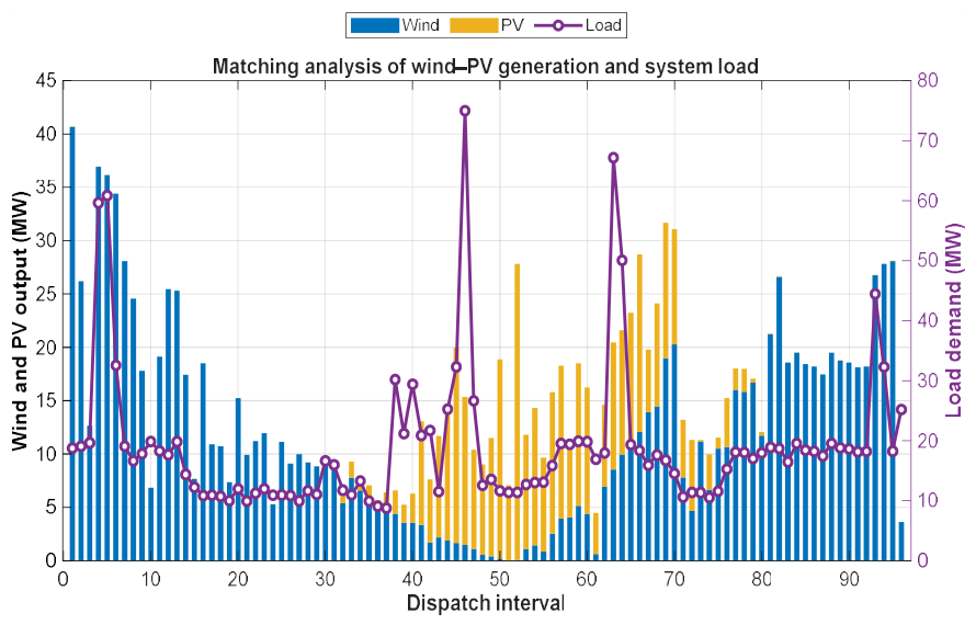
Figure 2 shows the wind power, PV power, and load profiles of a representative spring day. Wind power is relatively high during the early intervals, declines before midday, and then increases again in the later periods. By contrast, PV output is concentrated mainly around midday and remains nearly zero during nighttime hours. Compared with renewable generation, the load profile exhibits stronger short-term volatility and several sharp peaks, leading to a clear time-varying source–load mismatch over the dispatch horizon. In intervals with weak renewable output and high load demand, the system is more likely to face a local supply deficit and therefore requires flexible support from storage resources and constrained grid import. In intervals with relatively abundant renewable generation, the system gains greater flexibility for local renewable utilization and intertemporal energy shifting. These characteristics indicate that the considered scenario captures the essential operational challenge of direct renewable-to-load systems, namely the time-varying mismatch between renewable generation and local demand and the resulting need for coordinated storage-supported energy management.

Key system parameters are configured to reflect a practical direct renewable-to-load setting. The electrochemical energy storage system has been modeled as a lithium-ion battery with an energy capacity of 30 MWh, a maximum charge/discharge power of 15 MW, a charge/discharge efficiency of 95%, and an SOC range of [0.2, 0.9]. The hydrogen energy storage system consists of an electrolyzer with a rated power of 10 MW, a hydrogen tank, and a fuel cell with a rated power of 8 MW. The electrolyzer efficiency and fuel-cell efficiency are set to 75% and 60%, respectively. These values are adopted as representative system-level parameters for scheduling analysis according to reported hydrogen energy storage studies and efficiency ranges in the literature. Specifically, a hydrogen energy storage system with electrolyzer and fuel-cell efficiencies of 0.75 and 0.60 has been used in renewable generation and distribution-network planning studies [34]. In addition, PEM electrolyzer efficiencies are commonly reported within the range of 70–90% [35]. Therefore, the adopted efficiencies are used as typical scheduling-level assumptions rather than product-specific part-load efficiency curves. The hydrogen tank is specified by both its equivalent chemical energy capacity and the corresponding physical hydrogen inventory. In this study, the maximum equivalent hydrogen storage capacity is set to 20 MWh. Based on the higher heating value of hydrogen, H_HV = 39.4 kWh/kg, this corresponds to a maximum hydrogen inventory of approximately 507.6 kg. The energy-based capacity is used in the optimization model to maintain consistency with the power and energy balance equations, while the corresponding mass-based value is provided to clarify the physical scale of the hydrogen tank. A peak–flat–valley TOU tariff is used: peak hours (10:00–15:00 and 18:00–21:00) at 1.2 CNY/kWh, valley hours (23:00–07:00) at 0.4 CNY/kWh, and flat hours at 0.8 CNY/kWh. The adopted TOU tariff contains peak-price periods from 10:00 to 15:00 and from 18:00 to 21:00. It should be noted that the daytime peak-price period partially overlaps with the PV generation peak. Therefore, the tariff structure may strengthen the economic incentive for local PV self-consumption during midday. In this study, the TOU tariff is used to represent a practical price signal for demand-side operation, while the algorithmic value of the proposed method is not attributed solely to this price–PV coincidence. The scheduling problem still requires coordinated decisions under renewable variability, load variation, the no-power-export boundary, PCC import limits, battery SOC constraints, hydrogen conversion constraints, and inter-temporal storage dynamics.

The renewable curtailment penalty is set to 0.5 CNY/kWh, the storage O&M cost is 0.01 CNY/kWh, and the throughput-based wear cost is calculated using the model in Section 2.2.3. The electrolyzer and fuel-cell wear-cost coefficients in Equation (20) are both set to $0.01$ CNY/kWh.

For performance benchmarking, the proposed DDPG-based method is compared with MILP, GA, and a without-storage baseline.

4.2. Operation Results

To further reveal the operating characteristics of the direct renewable-to-load system under the no-power-export operating boundary, this subsection analyzes the coordinated source–load–storage regulation mechanism based on the MILP benchmark results. It should be noted that the battery charging/discharging exclusivity in the MILP benchmark is represented by the binary-variable linear formulation in Equations (7)–(9), rather than by directly imposing the nonlinear product constraint $P_{\mathrm{bat}}^{\mathrm{ch}}(t)P_{\mathrm{bat}}^{\mathrm{dis}}(t)=0$. Therefore, the benchmark problem remains a mixed-integer linear programming problem, and the reported MILP solution is interpreted as a full-horizon offline benchmark obtained within the specified solver tolerance. 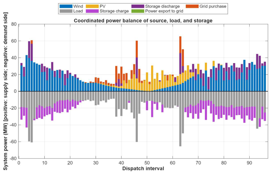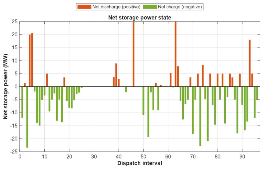Figure 3 presents the time-series power balance among wind power, PV power, load demand, and storage charging/discharging over a representative day, while Figure 4 further illustrates the storage operating state at each dispatch interval. It can be observed that the system maintains power balance mainly through direct renewable supply and intertemporal storage regulation, which reflects a typical operating pattern characterized by renewable-priority utilization and flexible storage response.

From the perspective of renewable generation, wind power remains relatively high during the early and late intervals but declines significantly during the middle part of the day. In contrast, PV generation is mainly concentrated around midday and exhibits several local peaks during the central dispatch periods. Compared with renewable generation, the system load stays at a moderate level for most intervals but shows several sharp spikes at specific times, resulting in a clear time-varying mismatch between supply and demand. During intervals with weak renewable output and rapidly increasing load, the system relies on storage discharge to compensate for the power deficit. By contrast, when wind–PV generation is relatively abundant and the load remains moderate, storage shifts to the charging state in order to absorb surplus renewable energy and reserve flexibility for subsequent high-demand periods.

As further shown in Figure 4, the storage system plays a significant role in intertemporal energy shifting throughout the representative day. On the one hand, during intervals with concentrated PV output or relatively abundant wind generation, storage charges continuously to enhance local renewable absorption and reduce curtailment. On the other hand, during load peaks or renewable output shortages, storage rapidly switches to the discharging state to smooth net-load fluctuations and alleviate supply pressure. This indicates that, under the no-grid-export operating boundary, storage does not follow a fixed charging/discharging pattern; instead, its operating state is dynamically adjusted according to source–load variations under the coordination of the optimization model, thereby improving the feasibility and flexibility of system operation.

In addition, the overall power-balance result in Figure 3 shows that, under storage power and energy constraints, the system may still experience local intervals in which renewable generation cannot be fully absorbed, leading to a certain amount of curtailment. This implies that direct renewable supply alone cannot completely eliminate temporal mismatch, and that storage sizing and dispatch strategy are crucial to improving renewable energy utilization. The operating patterns revealed by the MILP benchmark provide a clear reference for the subsequent comparison with DDPG, GA, and the without-storage case, and they also verify the necessity of establishing a coordinated source–load–storage scheduling mechanism under the no-power-export condition.

4.3. Comparison Between Single-Type and Multi-Type Storage Configurations

To further clarify the value of heterogeneous flexibility in the direct renewable-to-load system, this subsection compares the scheduling performance of different storage configurations under the same DDPG-based dispatch framework. Specifically, three storage-enabled cases are considered, namely battery-only storage, hydrogen-only storage, and coordinated battery–hydrogen storage. In addition, the without-storage case can be used as a reference benchmark to illustrate the necessity of introducing flexible resources. The comparison focuses on operating cost, renewable energy utilization, grid electricity purchase, renewable curtailment, and supply reliability. The comparison is conducted under a baseline operating-cost framework, without explicitly considering carbon pricing, renewable energy consumption incentives, or hydrogen-related subsidies.

Table 5. Comparison of Single-Type and Coordinated Battery–Hydrogen Storage Configurations.

Storage Configuration	Daily Operating Cost (×104 CNY/day)	Renewable Energy Utilization (%)
Battery-Only Storage	28.29	51.72
Hydrogen-Only Storage	32.36	52.19
Coordinated Battery–Hydrogen Storage	25.28	54.79

summarizes the overall scheduling performance under different storage configurations. Under the baseline operating-cost framework, the coordinated battery–hydrogen configuration achieves the best overall performance among the compared cases in terms of renewable energy accommodation and operating cost. The battery-only case is effective in mitigating short-term power fluctuations and reducing rapid source–load mismatch, but its energy-shifting capability is limited by battery energy capacity and frequent cycling requirements. By contrast, the hydrogen-only case provides a larger temporal buffer for surplus renewable energy, but its relatively slower dynamic response and lower round-trip efficiency limit its ability to handle fast intra-day variability. It should be noted that the relatively higher renewable utilization of the hydrogen-only case may have additional economic value if carbon pricing, green hydrogen subsidies, or renewable energy consumption incentives are introduced. Therefore, the current cost ranking should be interpreted within the adopted baseline cost boundary, rather than as a universal conclusion on the economic inferiority of hydrogen storage.

Therefore, under the selected case setting, the single-type storage configurations are less effective than the coordinated battery–hydrogen configuration in simultaneously providing short-term regulation and long-duration energy shifting.

The results in Table 5 indicate that storage configuration has a significant impact on both the operating economy and renewable energy utilization of the direct renewable-to-load system. Under the baseline operating-cost framework adopted in this study, which does not explicitly consider carbon pricing, renewable energy consumption incentives, or hydrogen-related subsidies, the coordinated battery–hydrogen storage configuration achieves the best overall performance among the three storage-enabled cases, with the lowest daily operating cost of 25.28 × 10⁴ CNY/day and the highest renewable energy utilization of 54.79%. In comparison, the battery-only storage case yields a daily operating cost of 28.29 × 10⁴ CNY/day and a renewable energy utilization of 51.72%. The hydrogen-only storage case achieves a slightly higher renewable energy utilization of 52.19% than the battery-only case, but its operating cost increases to 32.36 × 10⁴ CNY/day due to hydrogen conversion losses and hydrogen subsystem operating costs. Therefore, the higher cost of the hydrogen-only case should be interpreted within the adopted baseline cost boundary, rather than as a universal conclusion that hydrogen storage is economically inferior. If carbon prices, green hydrogen subsidies, or renewable consumption incentives are introduced, the additional renewable utilization and low-carbon value of hydrogen storage may be monetized, which could change the relative economic ranking of different storage configurations. Under the selected case setting, the coordinated use of battery and hydrogen storage can better exploit the complementary characteristics of the two technologies, thereby reducing operating costs while improving the accommodation capability of renewable energy.

To further interpret the internal coordination mechanism of the multi-type storage framework, the DDPG dispatch results for a representative spring day were examined.

Table 6. Comparison of Scheduling Performance between Battery Energy Storage and Hydrogen Energy Storage.

Metric	Battery Energy Storage	Hydrogen Storage
Average daily charging energy (MWh)	45.06	32.39
Average daily discharging energy (MWh)	40.67	13.30
Average daily cycles	1.36	0.67
Equivalent full-load hours (h)	2.71	1.66

presents the operational characteristics of the battery subsystem and the hydrogen subsystem in the coordinated case.

The apparent gap between the electrolyzer energy consumption and the fuel-cell output should be interpreted according to the energy conversion chain of the hydrogen subsystem. The electrolyzer energy of 32.39 MWh represents the electrical input for hydrogen production, while the fuel-cell energy of 13.30 MWh represents the regenerated electrical output. With an electrolyzer efficiency of 75%, the 32.39 MWh electrical input corresponds to approximately 24.29 MWh of hydrogen chemical energy. With a fuel-cell efficiency of 60%, the 13.30 MWh electrical output corresponds to approximately 22.17 MWh of consumed hydrogen chemical energy. Therefore, about 2.13 MWh of hydrogen chemical energy remains in the tank as a net increase in hydrogen inventory. The remaining difference is attributed to the electrolyzer conversion loss and fuel-cell conversion loss. Therefore, the difference between the reported hydrogen charging and discharging energies is not an unexplained energy loss, but results from conversion losses and inter-temporal hydrogen storage.

In addition, Table 6 shows that the two storage types exhibit a clear functional distinction in the coordinated scheduling framework. Battery storage mainly provides fast and flexible short-term regulation through more frequent charging/discharging responses, whereas the hydrogen subsystem mainly supports longer-duration energy shifting through gradual adjustment of stored energy. More specifically, when the power imbalance is short in duration or changes rapidly, the learned policy tends to regulate battery charging/discharging because the battery can respond quickly with relatively high round-trip efficiency. When renewable surplus lasts for a longer period and cannot be fully absorbed by the local load or battery within the SOC boundary, the policy increases electrolyzer operation to convert surplus electricity into hydrogen. Conversely, when renewable output remains insufficient and the load cannot be economically supplied by renewable generation and battery discharge alone, the fuel cell is dispatched to release stored hydrogen energy. This operating pattern indicates that the proposed method coordinates the two storage technologies according to their complementary temporal characteristics rather than treating them as identical energy buffers. This division of labor is consistent with the representative-day operating trajectories and explains why the coordinated multi-type storage configuration outperforms the single-type storage cases. Overall, the results confirm that coordinated scheduling of battery and hydrogen storage helps improve renewable energy utilization while reducing the operating cost of the direct renewable-to-load system.

This finding indicates that the coordinated use of electrochemical and hydrogen storage is particularly suitable for direct renewable-to-load systems, where no-power-export constraints and multi-timescale source–load mismatch coexist.

4.4. Comparison Among Different Optimization Methods

For a clearer benchmark interpretation, all compared methods were evaluated using the same deterministic renewable generation and load time-series data. This setting was adopted to ensure a controlled comparison under identical input conditions, rather than to demonstrate uncertainty robustness or to claim that DDPG is inherently more reliable than MILP under stochastic operating conditions. The four compared cases are assigned different roles in this study. MILP is adopted as a full-horizon offline benchmark solved within the specified solver tolerance, because it optimizes the scheduling problem over the complete horizon with model information and explicit operational constraints. It should be noted that in this study, the MILP benchmark is not implemented as a rolling online re-optimization method. Instead, it uses the given full-horizon time-series information to provide an offline reference for solution quality. GA has been selected as a representative meta-heuristic baseline to evaluate the performance of heuristic search. The without-storage case is used as a physical baseline to quantify the value of introducing flexible storage resources. By contrast, the proposed DDPG method is evaluated as an online scheduling policy after offline training, where dispatch actions are generated through fast state-feedback inference. Therefore, the MILP–DDPG comparison is intended to illustrate the trade-off between offline benchmark performance and online execution efficiency, rather than to claim that DDPG outperforms rolling MILP under identical online information conditions or under explicitly modeled uncertainty.

To make the MILP benchmark interpretation more rigorous, the solver settings and convergence information are reported here. The MILP model was solved using MATLAB R2025a intlinprog. The maximum solution time was set to 600 s, the relative MIP gap tolerance was set to 0.001, corresponding to 0.1%, the absolute gap tolerance was set to 10⁻⁶, the constraint tolerance was set to 10⁻⁶, and the integer tolerance was set to 10⁻⁵. In the reported case, the solver terminated with exitflag = 1. The final relative MIP gap was 0.000998383, corresponding to 0.0998%, and the final absolute MIP gap was 74.9321. The maximum constraint violation was 1.01773 × 10⁻¹³. Therefore, MILP is used in this study as a full-horizon offline benchmark solved within the specified solver tolerance, rather than as unconditional proof of exact zero-gap global optimality.

As shown in

Table 7. Performance comparison of different methods.

Method	Operating Cost (×104 CNY/day)	Renewable Energy Utilization Rate (%)	Computation Time (s)
MILP	18.76	57.22	16.47
GA	23.99	51.77	50.67
DDPG	20.93	55.00	0.25
Without Storage	32.15	43.59	0.0056

, MILP achieves the best full-horizon offline benchmark performance among the compared methods, with the lowest operating cost of 18.76 × 10⁴ CNY/day and the highest renewable energy utilization of 535.12 MWh. This result is expected because MILP optimizes the scheduling problem over the complete operating horizon with known time-series information and explicit constraints. However, this MILP result should be interpreted as an offline reference rather than a rolling online re-optimization result. Its computation time of 16.47 s indicates that frequent online re-optimization may introduce additional computational burden if MILP is implemented in a rolling manner.

GA yields an operating cost of CNY 23.99 × 10⁴/day, renewable energy utilization of 484.17 MWh, and computation time of 50.67 s. Compared with MILP, the GA result shows a higher operating cost and lower renewable utilization, indicating that the meta-heuristic search does not provide an advantage in solution quality in this representative case. In addition, under the current implementation, its computation time is longer than those of the reported MILP benchmark and DDPG inference, which weakens its suitability for fast online scheduling in this representative case.

The proposed DDPG method does not outperform MILP in full-horizon offline optimality, nor is it compared here against a rolling MILP implementation under identical online information conditions. Instead, the purpose of the comparison is to use MILP as an offline reference and to evaluate whether the trained DDPG policy can provide a computationally efficient online scheduling alternative with acceptable operating performance. In the representative test case, DDPG achieves an operating cost of CNY 20.93 × 10⁴/day and renewable energy utilization of 514.38 MWh. Compared with the full-horizon offline MILP benchmark, DDPG has an operating cost gap of approximately 11.6% and a renewable utilization gap of approximately 3.9%, while requiring a much shorter online inference time after offline training. However, this time comparison reflects different execution modes; MILP is solved as a full-horizon offline optimization problem, whereas DDPG generates actions through trained policy inference. Therefore, the result should not be interpreted as a direct runtime comparison against a rolling MILP implementation. This result indicates that the trained policy can provide a computationally efficient online scheduling alternative while maintaining acceptable operating performance.

Compared with GA, DDPG reduces the operating cost from CNY 23.99 × 10⁴/day to CNY 20.93 × 10⁴/day, corresponding to a reduction of approximately 12.8% in this representative test case. Meanwhile, renewable energy utilization increases from 484.17 MWh to 514.38 MWh, and the computation time decreases from 50.67 s to 0.25 s. These results suggest that, under the selected case setting, DDPG provides better overall performance than GA in terms of operating cost, renewable energy utilization, and online execution efficiency.

Compared with the without-storage baseline, DDPG reduces the operating cost from CNY 32.15 × 10⁴/day to CNY 20.93 × 10⁴/day and increases renewable energy utilization from 407.71 MWh to 514.38 MWh. This comparison demonstrates the operational value of flexible storage resources in the direct renewable-to-load system. By coordinating battery storage and hydrogen storage, the proposed method improves local renewable energy absorption and reduces the dependence on costly corrective measures.

It should be noted that both GA and DDPG contain stochastic components. GA is affected by the random initialization of the population and evolutionary operators, while DDPG is affected by neural-network initialization, exploration noise, and replay-buffer sampling during training. In this study, the comparison is conducted for a representative test case using the same input data, and the results are intended to illustrate the relative performance under the selected setting. Since repeated evaluations under multiple random seeds are not reported, the DDPG–GA comparison should not be regarded as a statistically significant conclusion. A more rigorous statistical assessment based on multiple independent random seeds will be conducted in future work.

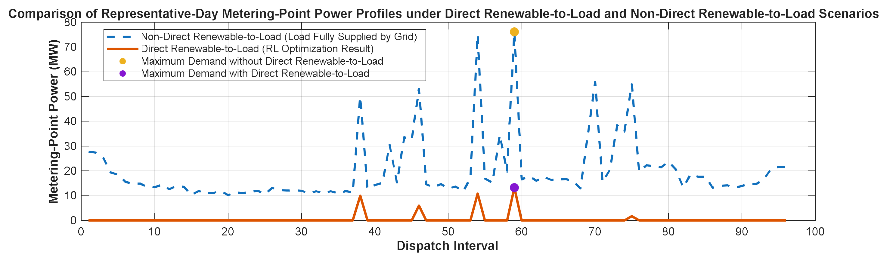
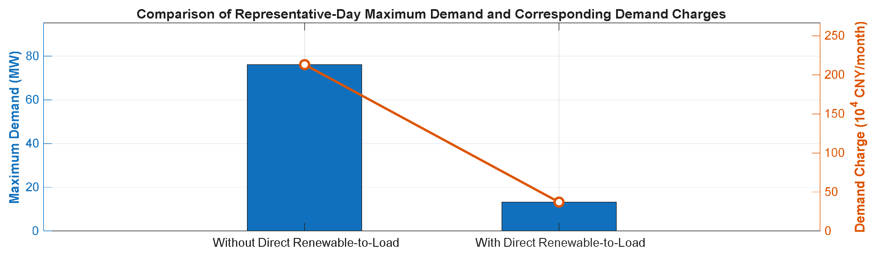
4.5. Representative-Day Demand Charge Indicator Analysis

Beyond operating cost and renewable energy consumption, the impact of the direct renewable-to-load mode on the user-side electricity cost structure also deserves attention. For energy-intensive industrial parks, the basic electricity charge is usually closely related to the maximum demand within the billing period. Therefore, reducing the grid-side purchased power peak at the public grid metering point can potentially lower the user-side demand charge and improve the overall economic performance of the system. However, since monthly demand charge is determined by the maximum demand over the entire billing cycle, a single representative day is not sufficient to provide a statistically validated monthly saving. Therefore, this section reports a representative-day maximum demand reduction indicator and provides an indicative demand-charge estimate rather than a generalized monthly saving.

On this basis, using the deep reinforcement learning-based dispatch model established in Section 3, this study compares the metering-point power profiles, maximum demand, and corresponding indicative demand charges of two scenarios: a direct renewable-to-load scenario and a non-direct renewable-to-load scenario. In the direct renewable-to-load scenario, the metering-point purchased power sequence is obtained from the DDPG-based optimization results. In the non-direct renewable-to-load scenario, under the same load condition, the park load is assumed to be fully supplied by the public grid, and the corresponding daily load profile is taken as the metering-point power sequence. To ensure a consistent comparison basis, a demand tariff of CNY 28/kW·month is adopted. The representative-day maximum demand is used as an indicative proxy for the monthly billing demand only for comparative illustration, and the resulting demand charge should not be interpreted as a statistically validated monthly saving.

To visually illustrate the differences in the metering-point power profiles and their peak values under the two scenarios, Figure 5 and Figure 6 present the comparison of the representative-day metering-point power profiles, as well as the statistics of the representative-day maximum demand and the corresponding indicative demand charges.

As shown in Figure 5, in the non-direct renewable-to-load scenario, the park load is entirely supplied by the public grid, leading to a relatively high metering-point power level and several pronounced peaks during high-load periods. By contrast, in the direct renewable-to-load scenario, wind power, PV generation, and energy storage jointly supply the park load, while the public grid only covers the residual deficit. As a result, the representative-day metering-point power profile is substantially reduced, and the peak value is effectively suppressed. This indicates that the direct renewable-to-load mode can alleviate the power burden at the metering point during the selected representative day, thereby providing a potential basis for reducing the user-side maximum demand.

As further shown in Figure 6, the representative-day maximum demand in the direct renewable-to-load scenario is 13.23 MW, which is lower than the 76.13 MW observed in the non-direct renewable-to-load scenario. This corresponds to a representative-day maximum demand reduction of 62.90 MW, or 82.6%. If the representative-day peak demand is used as an indicative proxy for the monthly billing demand, the corresponding demand charge decreases from CNY 2.1317 million/month to CNY 0.3705 million/month. However, this calculation should be interpreted only as an indicative demand-charge estimate under the representative-day proxy assumption, rather than as a statistically validated monthly saving.

Overall, the direct renewable-to-load mode shows clear potential to reduce the metering-point peak purchased power and improve the user-side electricity cost structure. Nevertheless, the present analysis is based on a single representative day and does not cover seasonal variation, full-month peak-demand distribution, or multi-day operational uncertainty. Therefore, the demand charge result is reported as a representative-day indicator. A rigorous monthly demand-charge assessment requires multi-day or full-month simulations considering seasonal renewable output and load variation, which will be investigated in future work.

4.6. Seasonal Performance Analysis

To further evaluate the influence of seasonal variations on the operation of the direct renewable-to-load system, representative days in spring, summer, autumn, and winter were selected from the measured dataset according to daily renewable generation, load level, and intraday fluctuation characteristics. The same trained DDPG scheduling policy was applied to the four seasonal representative days, and the main operation indicators are summarized in

Table 8. Seasonal representative-day performance of the proposed DDPG scheduling method.

Season	Operating Cost (CNY 104/day)	Renewable Energy Utilization Rate (%)	Grid Import (MWh)	Renewable Curtailment (MWh)	Battery Throughput (MWh)	Electrolyzer Energy (MWh)	Fuel-Cell Output (MWh)
Spring	20.93	55.00	286.42	420.86	73.18	32.39	13.30
Summer	23.64	58.26	331.75	386.24	82.47	29.58	16.72
Autumn	19.87	61.34	248.96	286.37	67.85	27.46	12.08
Winter	25.42	63.18	372.63	198.54	58.29	20.35	18.64

. For consistency with the preceding comparison tables, renewable energy utilization is reported as the renewable energy utilization rate.

As shown in Table 8, seasonal variations have a clear impact on the operation performance of the direct renewable-to-load system. In the spring representative day, renewable generation is relatively abundant, while the load level remains moderate. Under the strict no-power-export boundary, part of the renewable generation cannot be fully absorbed by the local load and storage devices, resulting in a relatively high curtailment of 420.86 MWh. Nevertheless, the coordinated battery–hydrogen storage strategy improves renewable absorption by using battery charging for short-term surplus smoothing and hydrogen production for longer-duration energy shifting.

In summer, both PV generation and load demand increase. The renewable energy utilization rate rises to 58.26%, indicating that the higher load level helps absorb part of the daytime renewable generation. However, the operating cost also increases to CNY 23.64 × 10⁴/day because the system still needs more grid import during high-load intervals, especially when renewable output cannot fully cover the load demand. The battery throughput reaches 82.47 MWh, which indicates that electrochemical storage is more frequently used for short-term power balancing under stronger intraday load fluctuations.

In autumn, the source–load matching condition is more balanced. The operating cost decreases to CNY 19.87 × 10⁴/day, and the renewable curtailment is reduced to 286.37 MWh. The renewable energy utilization rate reaches 61.34%, which is higher than that in spring and summer. This result indicates that a moderate renewable output level and relatively smooth load profile can improve local renewable absorption under the no-power-export constraint. In this case, the battery and hydrogen subsystems are still coordinated, but the overall storage regulation pressure is lower than that in summer.

In winter, renewable curtailment is further reduced to 198.54 MWh, and the renewable energy utilization rate increases to 63.18%. This is mainly because the available renewable generation is lower while the load demand is higher, allowing a larger proportion of renewable energy to be consumed locally. However, the operating cost reaches CNY 25.42 × 10⁴/day, which is the highest among the four representative days, due to the increased dependence on grid import. In addition, the fuel-cell output increases to 18.64 MWh, indicating that stored hydrogen plays a more important role in supporting the system during renewable-deficient and high-demand intervals.

Overall, the seasonal representative-day results show that the proposed DDPG-based coordinated scheduling method can adapt to different renewable generation and load demand patterns. During renewable-rich periods, the system mainly relies on battery charging and hydrogen production to absorb surplus renewable power and reduce curtailment. During periods with higher load demand or weaker renewable output, battery discharge, fuel-cell output, and grid import become more important for maintaining power balance. Therefore, the coordinated use of battery storage and hydrogen storage provides multi-timescale flexibility for the direct renewable-to-load system under seasonal source–load variations.

4.7. Sensitivity Analysis of Storage Wear-Cost Parameters

To further discuss the influence of storage aging-related parameters on the operation of the hybrid energy storage system, a sensitivity analysis is conducted by varying the operating wear-cost coefficients of battery storage and hydrogen storage. Since detailed electrochemical aging and degradation mechanisms are not explicitly modeled in this study, the sensitivity analysis focuses on the throughput-based wear-cost parameters used in the scheduling objective. Three cases are compared: the base case, the high battery wear-cost case, and the high hydrogen wear-cost case. In the high battery wear-cost case, the battery wear-cost coefficient is increased to represent stronger concern about battery cycling degradation. In the high hydrogen wear-cost case, the electrolyzer and fuel-cell wear-cost coefficients are increased to represent higher degradation or maintenance cost of the hydrogen subsystem. The results are summarized in

Table 9. Operation results under different storage wear-cost parameter settings.

Case	Operating Cost (CNY 104/day)	Renewable Energy Utilization Rate (%)	Grid Import (MWh)	Battery Throughput (MWh)	Electrolyzer Energy (MWh)	Fuel-Cell Output (MWh)
Base case	20.93	55.00	286.42	73.18	32.39	13.30
High battery wear cost	21.58	53.84	292.67	58.46	36.72	14.85
High hydrogen wear cost	21.34	54.21	296.08	80.39	24.16	9.42

.

As shown in Table 9, the storage wear-cost parameters have a clear impact on the coordination strategy of the hybrid energy storage system. When the battery wear-cost coefficient increases, the battery throughput decreases from 73.18 MWh to 58.46 MWh, indicating that the scheduler reduces frequent battery cycling to avoid excessive battery usage. Under this condition, the system tends to shift part of the surplus renewable energy to hydrogen production, and the electrolyzer energy increases from 32.39 MWh to 36.72 MWh. This result reflects the complementary role of hydrogen storage when battery cycling becomes economically less favorable.

When the hydrogen wear-cost coefficients increase, the operation of the hydrogen subsystem is reduced. The electrolyzer energy decreases from 32.39 MWh to 24.16 MWh, and the fuel-cell output decreases from 13.30 MWh to 9.42 MWh. In this case, the system relies more on battery charging/discharging and grid import to maintain the power balance. The battery throughput increases to 80.39 MWh, while grid import also increases to 296.08 MWh. This indicates that higher hydrogen subsystem wear cost weakens the long-duration energy-shifting function of hydrogen storage and increases the regulation burden on the battery and the grid.

Overall, the sensitivity results show that aging-related storage cost parameters affect not only the total operating cost, but also the allocation of regulation tasks between battery storage and hydrogen storage. Battery wear-cost increase suppresses high-frequency battery cycling and encourages more use of hydrogen energy shifting, whereas hydrogen wear-cost increase reduces hydrogen conversion and shifts more regulation demand to the battery and grid import. Therefore, accurate assessment of storage aging and wear-cost parameters is important for long-term operation planning of hybrid energy storage systems. In future work, more detailed degradation models considering battery cycle depth, temperature, calendar aging, electrolyzer start–stop degradation, and fuel-cell lifetime characteristics will be incorporated to further improve the long-term scheduling accuracy.

In addition to storage-parameter sensitivity, uncertainty factors may also affect the practical operation of the proposed scheduling framework. The present study is conducted using deterministic measured renewable generation, load demand, and electricity price time-series data, which provides a controlled basis for comparing different scheduling methods under identical input conditions. However, in practical operation, renewable generation forecast errors, load demand variations, and market price fluctuations may affect the performance of the direct renewable-to-load system. If actual renewable output is lower than expected, the system may require additional grid import, battery discharge, or fuel-cell output to maintain power balance. If actual renewable output is higher than expected, the no-power-export boundary may increase the risk of renewable curtailment unless sufficient storage flexibility is available. Similarly, unexpected load increases may increase the demand for storage discharge and grid import, while unexpected load reductions may lead to surplus renewable generation. Market price fluctuations may also change the economic timing of grid import, battery charging/discharging, and hydrogen conversion. The proposed DDPG scheduler has state-feedback capability because dispatch actions are generated according to observed renewable generation, load demand, battery SOC, hydrogen inventory, and time-related information. Nevertheless, the current framework does not explicitly model probabilistic forecasts, forecast-error histories, stochastic transition processes, or real-time price uncertainty. Therefore, the reported results should be interpreted as deterministic measured-data-based scheduling results rather than as a formal robustness evaluation under uncertainty. Future work will incorporate probabilistic renewable/load forecasts, stochastic price scenarios, and robust or risk-aware reinforcement learning methods to further evaluate the reliability of the proposed scheduling framework under uncertainty.

5. Conclusions

This paper investigates the operation optimization problem of a direct renewable-to-load system integrating battery energy storage and power-to-hydrogen facilities under practical grid-interaction limits and no-power-export constraints. By formulating the scheduling task as a Markov decision process and solving it with a DDPG-based coordinated control framework, the proposed method was able to explicitly capture the coupling among renewable generation, load demand, battery dynamics, hydrogen conversion, and constrained grid support.

The case studies demonstrate that coordinated heterogeneous storage plays an important role in improving the overall performance of direct renewable-to-load systems. In the storage-configuration comparison, the coordinated battery–hydrogen scheme outperformed both the battery-only and hydrogen-only cases, achieving the lowest daily operating cost of CNY $25.28\times {10}^4$/day and the highest renewable energy utilization of 54.79%. The analysis of storage operating characteristics further shows that battery storage mainly contributes fast and frequent short-term regulation, while the hydrogen subsystem provides smoother and longer-duration energy shifting. This complementarity explains why the coordinated configuration is more suitable than single-type storage for direct renewable-to-load operation with multi-timescale source–load mismatch.

The comparison among different optimization methods further confirmed the effectiveness of the proposed DDPG framework. Although MILP achieved the best offline benchmark performance, DDPG still maintained competitive operating results with an operating cost of CNY $20.93\times {10}^4$/day and a renewable energy utilization of 514.38 MWh, while significantly outperforming GA and the without-storage baseline with regard to overall balance between economy and flexibility. More importantly, DDPG required only 0.25 s/step for online inference, which highlights its suitability for fast rolling decision-making in practical applications. Therefore, the proposed method provides a promising data-driven solution for real-time operation optimization of direct renewable-to-load systems.

In addition, the direct renewable-to-load mode shows clear potential to reduce user-side demand charges by lowering the peak purchased power at the metering point, thereby providing additional economic support for its application in industrial park scenarios.

Although the proposed framework demonstrates promising performance in state-feedback-based online scheduling, several limitations remain to be addressed. One limitation of the current framework is that historical renewable forecast errors, probabilistic forecast information, and stochastic transition models are not explicitly included. Therefore, the proposed policy mainly responds to observed intra-day renewable generation and load variations through state feedback, rather than explicitly modeling forecast-error dynamics or robust uncertainty propagation. Extending the state representation and transition model to incorporate forecast-error histories, probabilistic forecasts, or stochastic disturbance processes will be an important direction for future work.

In addition, the current DDPG training process adopts a fixed exploration-noise setting. Although the exploration noise is used only during training and is removed during policy evaluation and online scheduling, a fixed noise level may affect exploration efficiency and convergence stability during the training stage. Future work will investigate decaying or adaptive exploration-noise schedules to further improve policy training stability and convergence performance under time-varying operating conditions.

Another limitation is that the current battery cost model adopts a throughput-based wear-cost approximation and does not explicitly account for cycle-depth-dependent aging, temperature effects, C-rate effects, or calendar degradation. Future work will incorporate more detailed aging-aware battery degradation or wear-cost models to improve the physical fidelity of long-term storage scheduling.

In addition, the current MILP benchmark is implemented as a full-horizon offline reference rather than as a rolling online re-optimization method. Therefore, the MILP–DDPG comparison in this study is intended to illustrate the trade-off between offline benchmark performance and online execution efficiency, rather than to claim that DDPG outperforms rolling MILP under identical online information conditions. Future work will include rolling MILP or model predictive control benchmarks under the same information-update setting to further evaluate the online performance of the proposed DDPG policy.

In addition, the current case study adopts a fixed TOU tariff structure, in which the daytime peak-price period partially overlaps with the PV generation peak. Future work will further evaluate the proposed method under different tariff structures, including shifted peak-price periods, flat tariffs, and real-time prices, to separate the effect of price signals from the intrinsic value of the scheduling algorithm.

Moreover, the current demand-charge analysis is based on a representative-day evaluation rather than a full-month simulation. Since monthly demand charge is determined by the maximum demand over the entire billing period, future work will extend the analysis to multi-day and full-month simulations to consider seasonal renewable generation, load variation, and monthly peak-demand uncertainty.