Article

A Non-Intrusive Load Identification Method Based on the Fusion of Steady-State Features and Lightweight Network


1
Sydney Smart Technology College, Northeastern University at Qinhuangdao, Qinhuangdao 066004, China
2
School of Computer and Communication Engineering, Northeastern University at Qinhuangdao, Qinhuangdao 066004, China
*
Author to whom correspondence should be addressed.
Energies 2026, 19(13), 3131; https://doi.org/10.3390/en19133131
Submission received: 30 May 2026 / Revised: 24 June 2026 / Accepted: 30 June 2026 / Published: 1 July 2026

Abstract

Non-intrusive load monitoring (NILM) is essential for smart grid demand-side management and energy conservation, yet existing methods suffer from limited feature discrimination, ambiguous identification of similar electrical appliances, and difficulty balancing model accuracy and lightweight deployment. To address these issues, this paper proposes a dual-branch lightweight load identification method fusing steady-state features and lightweight network. Firstly, V-I trajectory images are generated via standardized transformation and two-dimensional histogram logarithmic mapping, while steady-state characteristics, including active power, reactive power, trajectory area and intermediate section slope, are extracted. Then, a dual-branch network is constructed, where the visual branch adopts depthwise separable convolution and lightweight multi-head attention to mine global trajectory features, and the numerical branch uses fully connected layers to encode steady-state features; feature concatenation fusion is adopted to complete appliance classification. The experimental results on the Plug Load Appliance Identification Dataset (PLAID dataset) show that the proposed method achieves a recognition accuracy of 95.35% with only 0.17M parameters, outperforming standard and medium convolutional neural network (CNN) models. Ablation experiments verify that steady-state feature fusion effectively improves the identification accuracy of easily confused and small-sample loads. The proposed method realizes high-precision and lightweight load identification, which is suitable for edge deployment in smart meters and has practical application value for intelligent power management.

1. Introduction

Energy acts as the fundamental driver of economic growth and social operation. Driven by global electrification expansion and rising household appliance ownership, overall energy and electricity demand maintain sustained upward momentum, yet the growth pace shows distinct structural shifts in recent years. According to the latest complete dataset covered in the Global Energy Review 2026, released by the International Energy Agency (IEA), global total energy demand rose by 1.3% in 2025, a notable slowdown compared with the 2.0% growth recorded in 2024, mainly restrained by decelerating expansion of energy-intensive industries, milder cooling demand and accelerated energy efficiency gains [1]. Notably, electricity demand grew at nearly 2.3 times the rate of total energy demand at approximately 3%, marking the official arrival of the global “Age of Electricity”; renewable photovoltaic power contributed more than one-quarter of the incremental energy demand, revealing an unprecedented energy transition trend [1]. Despite the booming deployment of clean energy, the construction of novel power systems still confronts the following two prominent bottlenecks: large-scale energy storage equipment lacks economic competitiveness at present, severely limiting the flexible regulation capacity of power grids; meanwhile, end-user electricity demand presents violent time-varying volatility [2]. This backdrop raises an urgent core research proposition: how to elevate terminal energy utilization efficiency and substantially cut avoidable energy waste [3].
As a vital component of smart grids, intelligent electricity management systems aim fundamentally to meet various IoT-based sensing and management needs on the user side, making them a key link in the development of smart IoT and digitalized power grids. Accurately and reliably acquiring load consumption data forms the foundation of intelligent electricity management [4]. In recent years, load monitoring technologies have attracted considerable attention from academia [5]. This is because such technologies can significantly improve energy-saving outcomes, facilitate energy efficiency monitoring and demand-side management, and guide users toward optimizing their electricity usage behaviors to reduce energy waste [6].
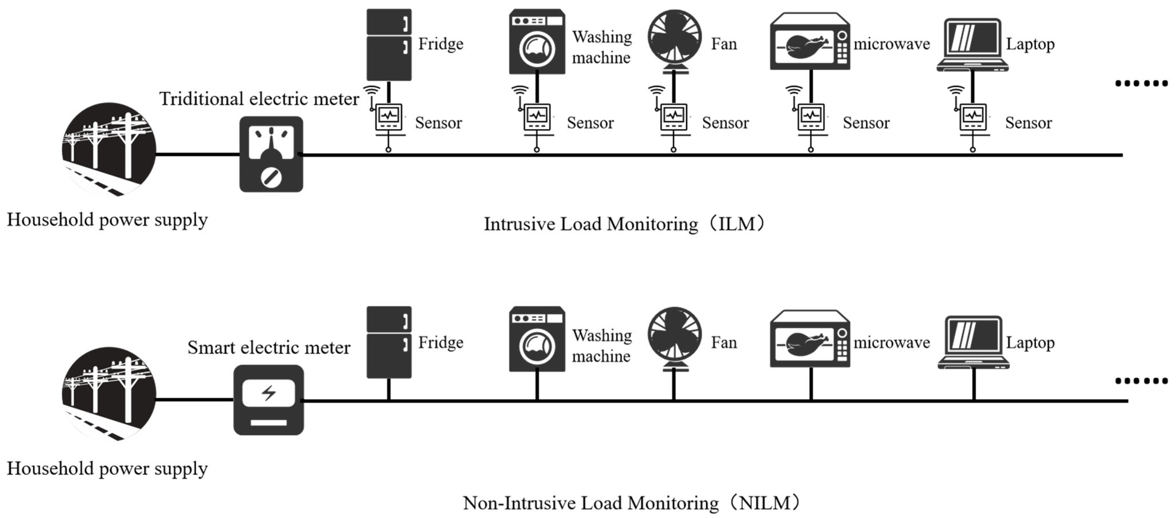
Depending on implementation methods, load-monitoring technologies can be divided into the following two categories: intrusive load monitoring (ILM) and NILM. As shown in Figure 1, ILM requires installing individual sensors on each electrical appliance to obtain detailed consumption data, thus ensuring highly reliable load information for each device. However, this method faces practical challenges such as difficult installation, inconvenient maintenance, and high costs. More seriously, it may infringe upon user privacy, limiting its practicality [7]. In contrast, NILM only requires installing a single smart meter at the user’s power entry point to collect total electricity data, then using appropriate algorithms to decompose the data into individual appliance consumption patterns without requiring separate sensors for each device [8]. This approach offers low-cost, simple installation. As a result, it has been widely applied in fields such as smart grids and energy-efficient buildings [9].
One of the fundamental tasks of NILM technology is load identification, which is to reliably and accurately identify the type of electrical appliances in operation at a given time from the total electricity consumption data. Therefore, the results of load identification have very clear and important application value: it is beneficial for users to obtain detailed energy consumption reports and energy-saving suggestions, for power grid companies to conduct analysis of users’ electricity usage behavior to support demand-side response and load forecasting, and also for electrical appliance manufacturing enterprises to obtain the real data of users’ use of products to guide product optimization design [10]. Therefore, the research on high-precision and lightweight methods for load identification of household appliances has extremely strong theoretical value and practical significance.
The theoretical prototype of NILM technology originated from the pioneering work of Professor Hart’s team at the Massachusetts Institute of Technology in 1992: The team proposed a finite state machine mathematical model, and then through rigorous mathematical derivation and algorithm verification, successfully established the technical path of NILM, that is, using the total electricity consumption information of all loads to infer and estimate the individual electricity consumption of each appliance [11]. Therefore, the work of Professor Hart’s team was not only a foundational research in this field but also actually promoted the research trend in NILM in academic circles, and subsequently emerged a large number of new methods and algorithms [12,13,14].
The development of load feature extraction research can be divided into several clear stages: Early research mainly utilized steady-state power characteristics. Professor Hart was the first to use the active power difference value as a load feature for appliance identification [10]. However, later as the types of appliances increased and the electricity usage scenarios became increasingly complex, a single power characteristic could not reliably distinguish appliances with similar power, so researchers began to actively seek more-dimensional features. Nakano et al. [15] proposed the analysis technology of power frequency periodic current signal features in 2006, first performing a fast Fourier transform spectral decomposition on the current waveform, thereby accurately extracting the high-order harmonic features of electrical equipment. In addition, Srinivasan et al. [16] used artificial neural networks to classify multiple parameters, simplifying complex parameters, thereby significantly improving the identification efficiency and accuracy, thus forming an excellent supplement. In more recent times, Gillis et al. [17] established a new load feature characterization system using wavelet transformation, which significantly improved the feature discrimination degree of different electricity-consuming devices.
Since reactive power is reasonably and naturally incorporated as a supplementary feature into the load identification problem, the joint analysis of active and reactive power can clearly distinguish resistive, inductive, and capacitive loads [18]. The V-I trajectory features directly present the impedance characteristics of electrical appliances in the form of a dynamic relationship curve within one cycle of voltage and current. Du et al. [19] proposed a three-dimensional tensor feature of point-by-point multiplication, addition, and subtraction of voltage and current, ingeniously expanding the feature dimension of the trajectory. This is complemented by Xie et al. [20] who encoded power and instantaneous information into the RGB three channels to obtain a color V-I trajectory image. Through these studies, it can be concluded that the fusion of multimodal features is beneficial for improving the accuracy of load identification.
Therefore, many scholars have conducted research on multimodal feature fusion. Li Peng et al. [21] first combined the theory of Fourier transform decomposition of steady-state current with the principle of frequency-domain superposition of bus current, establishing an optimized solution model to determine the optimal equipment switching combination. Liu et al. [22] proposed a NILM method based on the improved crow search algorithm, which forms a good complement to this. Song et al. [23] started from the power quality monitoring data, extracted specific frequency band harmonic components, used the Adaboost algorithm to conduct secondary screening of current features, and then used the kernel linear discriminant method to design classification systems for different household appliances. Some scholars combined the V-I curve with the harmonic steady-state characteristics, and through the improvement of the ant colony algorithm, they optimized LightGBM to build an ACO-LightGBM non-intrusive load identification model to obtain the appliance start-stop labels. This effectively improved the prediction error of load sudden changes caused by the switching of high-power appliances [24]. Additionally, Liu et al. [25] proposed a decision-making layer fusion framework. They extracted one-dimensional power steady-state numerical features and binary V-I trajectory image features respectively. Through diversity indicators, they selected complementary machine learning base learners, combined with Swin Transformer to process the image features, and utilized information entropy to adaptively allocate the voting weights of each model to complete the integrated identification.
Since traditional machine learning methods such as support vector machines, K-nearest neighbors, and random forests have already had very reliable and mature application results in small sample cases [26,27,28], it can be observed that using LightGBM, which is a gradient boosting decision tree framework that utilizes histogram algorithms and leaf growth strategies, performs extremely well in handling high-dimensional features and large sample data [29].
Due to the development of deep learning, convolutional neural networks, which have excellent image feature extraction capabilities, become a tool for V-I trajectory image classification. Therefore, De Baets et al. [30] gridified the V-I trajectory and input it into CNN for load classification, achieving excellent results on the PLAID dataset. Kelly et al. [31] was the first to formally and systematically introduce deep learning methods into the NILM field, proposing an end-to-end CNN architecture. Zhang et al. [32] proposed a sequence-to-point learning paradigm, achieving outstanding performance on the REDD dataset. To improve model performance, Gu [33] designed a multi-head attention CNN model optimized by Bayesian optimization to complete the classification of V-I trajectory electrical appliances. Moreno et al. [34] constructed a CNN basic model based on VGG16 and MobileNet through transfer learning, and proposed the weighted confidence average voting (WeCV) integration strategy to fuse the prediction results of multiple models. Furthermore, Kulathilaka et al. [35] constructed a deep neural network for NILM that integrates WaveNet, seq2seq and time series ensemble learning, achieving precise decomposition of various types of loads in commercial buildings and online visualization of energy consumption.
Since lightweight model design is currently a very active and important research direction, various methods such as depth separable convolution and channel shuffling have been naturally and reasonably used to design lightweight networks [36]. Ma et al. [37] proposed ShuffleNet V2, effectively achieving efficient feature extraction using channel splitting and channel shuffling techniques. In addition, Wang et al. [38] designed a lightweight V-I trajectory feature extraction network based on depth separable convolution and channel shuffling, maintaining high accuracy while significantly reducing the number of parameters, both of which directly assist the deployment of load identification on edge devices. Abu Sbeitan et al. [39] proposed a lightweight feature extraction framework that integrates phase space reconstruction and two-dimensional Fourier descriptors. Dong et al. [40] proposed the TVDR-TDWS transient separation preprocessing method and the lightweight FSC-FS-Net network to address the issues of large parameter quantities in existing NILM models, the signal aliasing caused by multiple load superimposition, and the difficulty in deploying on edge devices. Serna et al. [41] studied the computing power, resource consumption and real-time inference performance of the NILM algorithm on edge embedded devices, and evaluated the feasibility of the NILM algorithm’s practical deployment at the edge.
From a systematic analysis of the current research status of non-invasive load identification, several shortcomings in this field can be summarized as follows:
  • Due to the poor discrimination of the characteristics of each measured load, the V-I trajectories of hair dryers and heaters, as well as those of different brands of refrigerators, are very similar. Therefore, the model is prone to misjudgment. For example, the V-I trajectory shapes of air conditioners and fans are extremely similar, and it is extremely difficult to distinguish them based on a single feature.
  • Due to the limitations of single-modal feature information, when using power features or V-I trajectory features to represent the electrical characteristics, it is inevitable that they cannot fully and reliably reflect the electrical characteristics, especially for multi-state complex electrical appliances. The information content of a single-modal feature is still insufficient to support accurate classification. Specifically, the power of microwave ovens and electric kettles is close, but their harmonic features are very different. Therefore, a single power feature cannot well distinguish them.
  • Due to the inability to achieve both high accuracy and efficiency in deep learning models, high-precision models generally use deep networks, which have large parameter quantities and high computational complexity. Therefore, it is difficult to directly deploy them on edge devices with extremely limited resources, while lightweight models necessarily sacrifice accuracy. As mentioned in Table 4 of Reference [35], for instance, the parameter quantities of neural network models such as Convolutional Neural Network and AlexNet are all greater than 20M, while the parameter quantity of the lightweight model used is approximately 1.07M. Therefore, this paper hopes to build upon Reference [35], without sacrificing too much accuracy, and reduce the parameter quantity of the lightweight model to below 1M.
  • Due to the extremely unbalanced distribution of samples in the PLAID dataset, for example, there are only 26 samples for washing machines, while there are 180 samples for energy-saving lamps, the sample imbalance naturally leads to the model’s bias towards most classes and poor recognition of minority classes.
  • Due to the insufficient attention of the academic community to model lightweighting, most existing literature focuses on improving recognition accuracy without considering the feasibility of deploying the designed model on edge devices. Therefore, there is a lack of analysis of parameter and computational quantities.
More specifically, in the direction of multimodal feature fusion, Du et al. [19] and Xie et al. [20] only constructed color V-I trajectory images, did not extract trajectory geometric steady-state descriptors, and only combined a single active and reactive power as auxiliary features. They lacked multi-dimensional geometric feature constraints and were unable to distinguish trajectory shapes of loads such as heaters and hair dryers that were highly similar; Li Peng et al. [21] combined frequency domain harmonic features with bus current superposition rules, but discarded spatial information of trajectory images, and insufficiently characterized the features of rectifier-type loads such as laptops. In terms of lightweight network architectures, Wang et al. [35] built a lightweight network based on depthwise separable convolution, but there is still room for further compression of model parameters, and they significantly reduced the number of multimodal steady-state numerical features, sacrificing the classification accuracy of minority class imbalanced samples; while ShuffleNet V2 uses channel shuffling to achieve lightweight optimization [34], but the frequent channel rearrangement operations introduce additional computational latency, which cannot meet the real-time inference requirements of low-cost smart meters. Moreover, most of the existing lightweight NILM models remove the attention module to reduce computational load, unable to explore the global symmetric spatial correlations within V-I trajectories, and this feature is the core visual discriminative basis for distinguishing similar appliances.
Thus, this paper proposes a dual-branch lightweight load identification model based on fused steady-state features, consisting of a V-I trajectory feature extraction branch and other steady-state feature extraction branches. The image branch uses three-layer convolution to extract various features such as the edges, local shapes, and global morphologies of the trajectory, and introduces a lightweight multi-head attention mechanism to extract the spatial dependencies and symmetrical patterns of the trajectory. Compared with reference [19] and reference [20], this paper employs a more diverse set of steady-state feature branch, which uses multi-layer fully connected networks to perform nonlinear encoding of power and digital features. The features extracted by the two branches are concatenated and fused before being sent to the classifier to obtain the probability of electrical categories. In this model, global average pooling is used instead of the traditional fully connected layer. In addition to using depthwise separable convolution [35], this paper also uses channel reduction strategy, so the parameter quantity is extremely well compressed, and the corresponding training strategy has also been discussed in detail.

2. Materials and Methods

2.1. Data Preprocessing

2.1.1. Dataset and Original Data

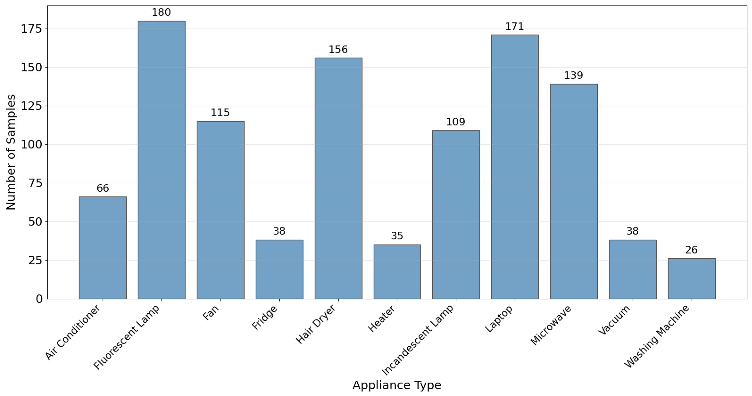
This study uses the PLAID dataset, which samples voltage and current waveforms at a frequency of 30 kHz. It contains over 1000 usable records covering 11 common household appliances, including incandescent lamps, laptops, vacuum cleaners, refrigerators, hair dryers, fans, heaters, energy-saving lamps, air conditioners, microwaves, and washing machines. The specific distribution of the original categories is shown in Figure 2.
Traditional NILM datasets generally focus on the analysis of steady-state characteristics, while the PLAID dataset centers on the transient electrical characteristics exhibited during the startup of electrical appliances, which provides strong data support for load identification research based on V-I trajectories. However, the number of samples in each category of this dataset is unbalanced: for example, the number of samples for appliances such as refrigerators and washing machines is relatively small, while the number of samples for appliances such as laptops and hair dryers is relatively sufficient. This situation brings certain challenges to model training and subsequent evaluation work.
Since the load data used in this article is the sampled data of voltage and current over time, the data files of each electrical appliance all provide complete instantaneous voltage and instantaneous current data within the power frequency period, with the sampling points being N. Therefore, the original data is presented as follows:
V = v 1 , v 2 , , v N T , I = i 1 , i 2 , , i N T
Among them, v k and i k represent the voltage and current values of the k-th sampling point respectively.

2.1.2. V-I Trajectory Generation Algorithm

The following text provides a detailed description of each step of the V-I trajectory generation algorithm.
1.
Data standardization
First, the voltage and current sequences are standardized to eliminate the influence of differences in units and amplitudes:
v ˜ k = v k μ v σ v + ϵ , i ˜ k = i k μ i σ i + ϵ
Among them, μ v = 1 N k = 1 N v k , μ i = 1 N k = 1 N i k represents the mean value;
σ v = 1 N k = 1 N v k μ v 2 , σ i = 1 N k = 1 N i k μ i 2 represents the standard deviation;
ϵ = 10−8 is a small constant, which is used to prevent division-by-zero errors.
2.
Amplitude clipping
To prevent the influence of outliers on the subsequent grid mapping, the standardized data will be clipped to a fixed range:
v k = clip v ˜ k , V max , V max , i k = clip i ˜ k , I max , I max
Among them, V max = I max = 2 , the clipping range is [−2, 2], which covers the majority of the standardized data points.
3.
Generation of 2D Histogram
The voltage-current space is divided into a G × G grid (in this paper, G = 28), and the width of each grid cell is δ = 4 / G . For each sampling point ( v t , i t ), determine the grid cell it belongs to and accumulate the count:
H u , w = k = 1 N 1 v k bin u , i k bin w
Among them, bin u = 2 + δ u 1 , 2 + δ u ;   u , w = 1 , 2 , , G ,   1 is the indicator function.
4.
Logarithmic Transformation
Due to the significant differences in the density of sampling points in different regions, directly using the original counts would result in an overly wide range of values. Therefore, a logarithmic transformation is applied to compress the counts:
H log u , w = ln 1 + H u , w
Logarithmic transformation has the following advantages:
(a) It compresses the data range, improving the stability of model training;
(b) It enhances the signals in low-density areas, preserving the detailed information of the trajectory;
(c) Maintain the monotonicity of the data.
5.
Normalization
Finally, the V-I trajectory image is normalized to the range of [0, 1] to serve as the input of the model:
X u , w = H log u , w max H log + ϵ
Among them, ϵ = 10−8 is a small constant used to prevent division-by-zero.
In this paper, the grid size G = 28 is preliminarily selected based on empirical trials. To quantitatively analyze the influence of grid resolution on model recognition performance, we set three groups of grid parameters G = 14, 28, 56 for sensitivity ablation experiments under identical network and training hyperparameters.
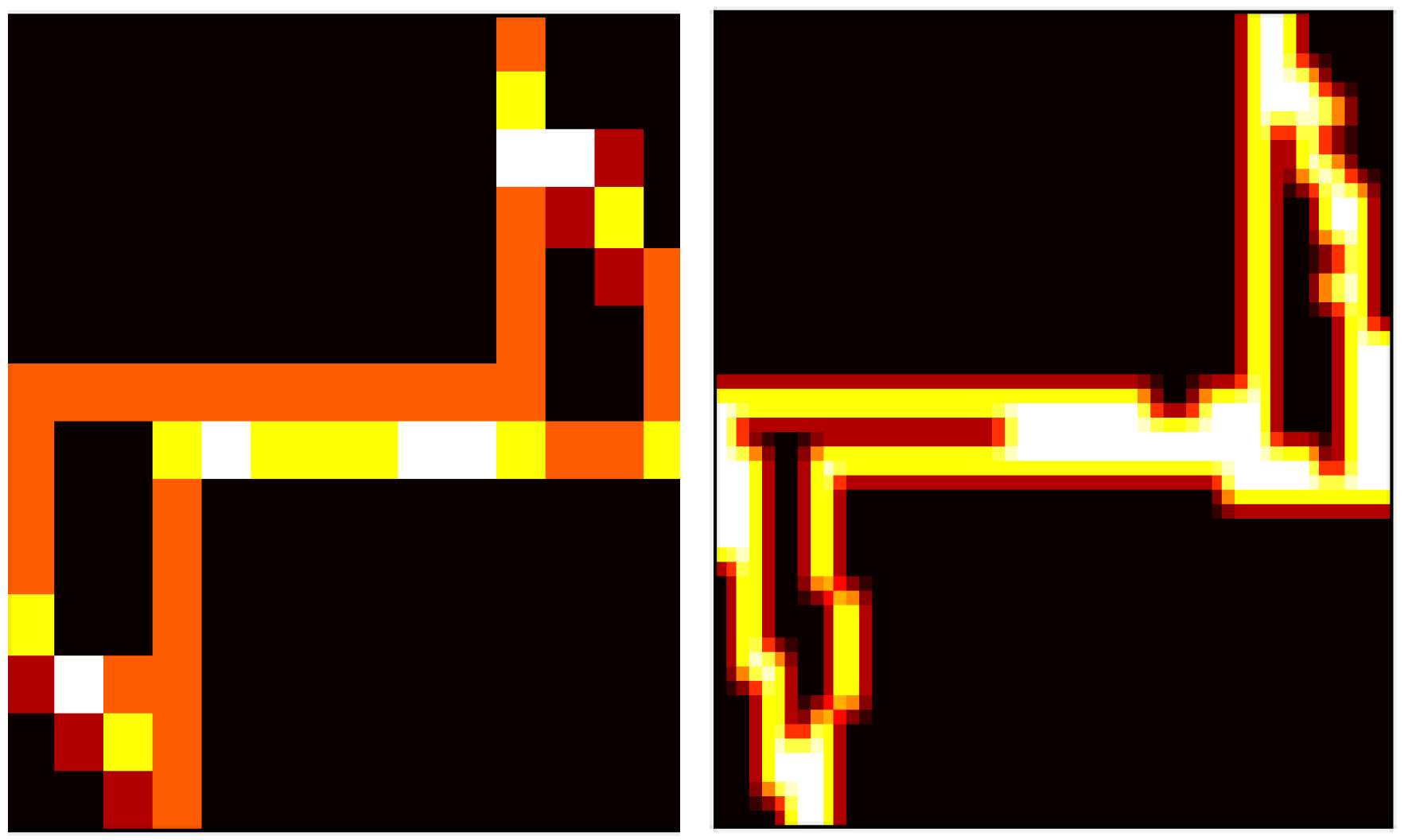
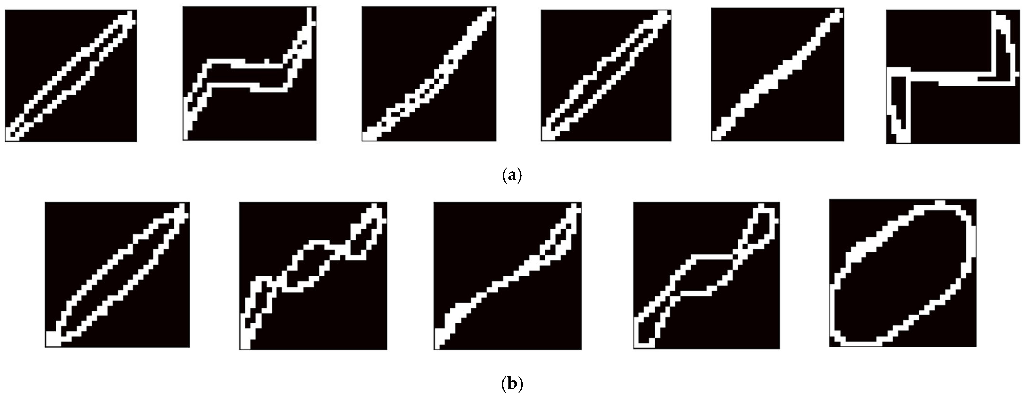
Firstly, taking energy-saving lamps as an example, the V-I curve diagrams for G = 14 and 56 are shown in Figure 3. Compared with the V-I curve characteristics of G = 28 in Figure 4, we can observe that when G = 14, the image is significantly distorted and lacks details. However, for G = 28 and G = 56, the overall details of the images are almost the same. The specific test results are shown in Table 1.
The grid of 14 × 14 achieves the smallest model parameters and fastest inference speed, yet severe loss of V-I trajectory details leads to the lowest test accuracy of 88.84% and Macro F1 of 81.80%. For 56 × 56 grid, higher resolution introduces redundant high-frequency noise, resulting in degraded generalization performance, with accuracy and Macro F1 dropping to 92.98% and 89.03%. Meanwhile, its parameters and inference time increase significantly, which raises deployment pressure on edge devices.
In contrast, the 28 × 28 grid obtains the optimal recognition performance, with the highest test accuracy of 94.42% and Macro F1 of 90.59%. Its model parameters only slightly rise to 0.17M with negligible memory overhead, and the inference latency is merely 0.5600 ms, which can fully meet the real-time requirement of non-intrusive load monitoring. Considering the trade-off among recognition accuracy, model lightweight and inference efficiency, the grid size G = 28 is selected for subsequent experiments in this paper.
The V-I curves of different types of electrical appliances generated by this algorithm are shown in Figure 4. And the summary of the distinguishable trajectory characteristics of each level of different appliances is presented in Table 2:

2.1.3. Other Steady-State Feature Extraction

1.
Power Feature Extraction
The power characteristics are mainly divided into active power and reactive power. In an alternating current circuit, active power is equivalent to the power consumption of resistive loads, that is, the average value of instantaneous power over one cycle, and it is also the most direct and reasonable measurement indicator for the actual output capacity of electrical equipment.
Since the voltage and current signals collected have been provided, the calculation formula for active power is:
P = 1 T 0 T v t i t dt
Since in actual discrete systems the solution needs to be obtained through numerical integration, the numerical integration calculation formula adopted is:
P = 1 N n = 1 N v n i n
Reactive power does not perform work externally nor is it actually consumed by the load; instead, it periodically exchanges back and forth between the source and the load over each AC cycle. Although reactive power itself does not produce mechanical or thermal effects, it plays a crucial role in ensuring the stable operation of AC systems.
The formula for calculating reactive power is:
Q = 1 T 0 T v t i t T 4 dt
In actual discrete systems, the numerical integration calculation formula is:
Q = 1 N n = 1 N v n i n N 4
2.
Digital Feature Extraction of V-I Trajectory
In addition to image features and power features, the V-I curve can also extract geometric features such as current span, curve area, cycle direction, number of intersection points, and slope of the middle section for load identification. Through experimental testing, this paper finally chose the curve area and the slope of the middle section to meet the feature identification requirements.
Given that the V-I curve exhibits a closed loop characteristic, its area calculation method can be derived using Green’s Theorem. The area enclosed by the closed curve can be calculated by using the coordinates of the discrete sampling points:
A = 1 2 k = 1 n V k I k + 1 V k + 1 I k
Among them, V k represents the voltage value of the kth sampling point,   I k represents the current value of the kth sampling point, and n represents the total number of sampling points. And it satisfies the closed condition: V n + 1 = V 1 ,   I n + 1 = I 1 . If the V-I trajectory has self-intersection situations, then the areas of each closed sub-region need to be calculated separately and summed up.
To avoid the strong nonlinear V-I curve, this paper employs the principal component analysis. Different from the local fitting of fixed intervals, the PCA global slope uses all voltage–current sampling points of the complete trajectory to implement global linear fitting, eliminating artificial segmentation bias. Given a set of trajectory sampling points V k , I k , k = 1 , 2 , , n , the calculation steps are as follows:
β pca = Cov I , I Cov V , V + Cov V , V Cov V , I 2 + 4   Cov ( V , I ) 2 2   Cov V , I
Among them, β pca corresponds to the gradient of the maximum variance direction of the V-I two-dimensional point cloud, which reflects the overall impedance characteristic of the load without being restricted by local segment selection. Cov V , I , Cov I , I and Cov V , V are the covariance terms of voltage and current.
1.
Data Preprocessing Procedure
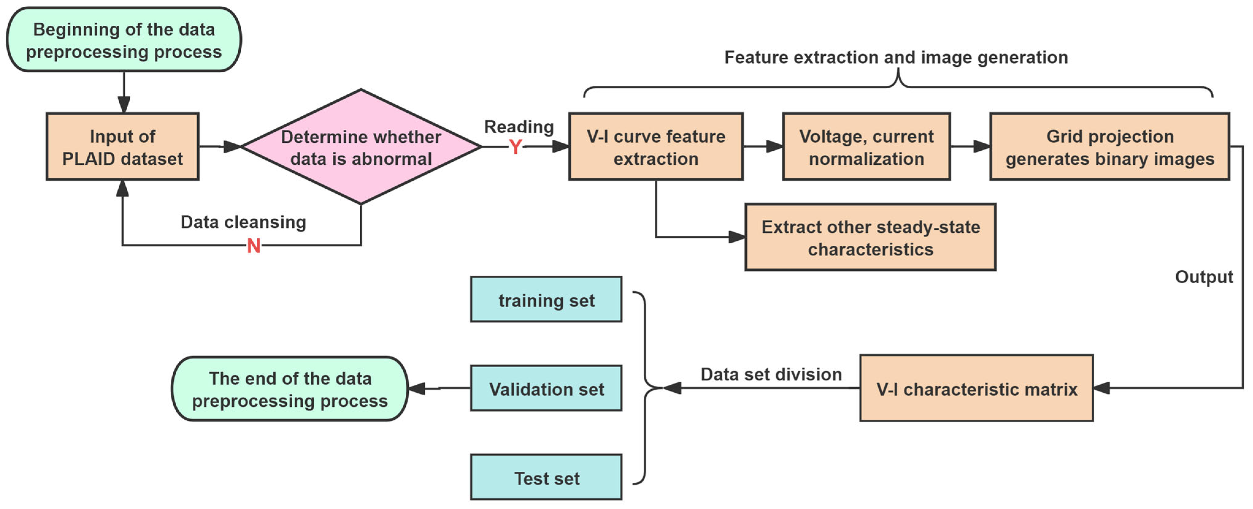
The complete preprocessing process is shown in Figure 5. The specific steps are as follows:
(1) Data Reading and Cleaning
This paper uses the publicly available PLAID dataset, which includes 11 types of household appliances and a total of 1074 samples. Each sample provides time series data of voltage and current within the power frequency cycle, with a sampling rate of 30 kHz. Due to the problems of uneven distribution of samples of different categories and some noise interference in the dataset, this paper first performs data reading and cleaning on the data, and finally obtains 1073 usable samples.
(2) Feature Extraction and Output
This paper first extracts the V-I trajectory from each sample in the PLAID dataset, then normalizes the voltage and current data, then projects these data onto a grid to generate a binary image, and finally outputs a 28 × 28 V-I trajectory matrix.
(3) Dataset Division
After outputting the V-I trajectory matrices of all samples, this paper conducts dataset division.
Figure 5. Data preprocessing flowchart.
Energies 19 03131 g005
2.
Data Set Partitioning Strategy
This paper randomly shuffles the dataset to ensure the randomness of the sample distribution. Then, it divides the dataset into a training set (80%) and a test set (20%) using stratified sampling. Subsequently, the training set is further divided into a training set (80% × 75% = 60%) for learning model parameters and a validation set (80% × 25% = 20%) for hyperparameter tuning and early stopping monitoring. This ensures that the proportion of each category is consistent, and the test set for the least frequent category also has at least 5 samples.

2.2. Load Identification Model

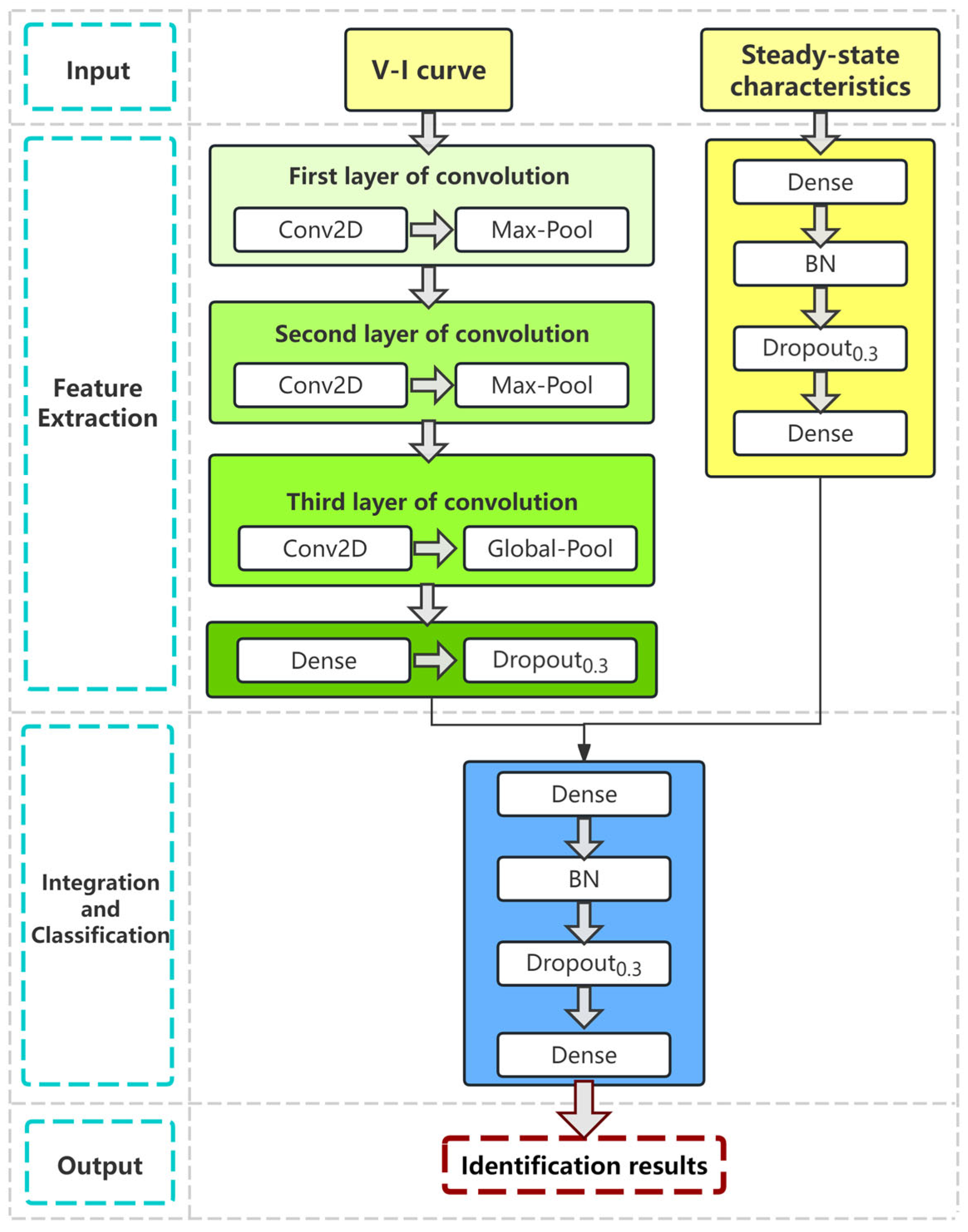
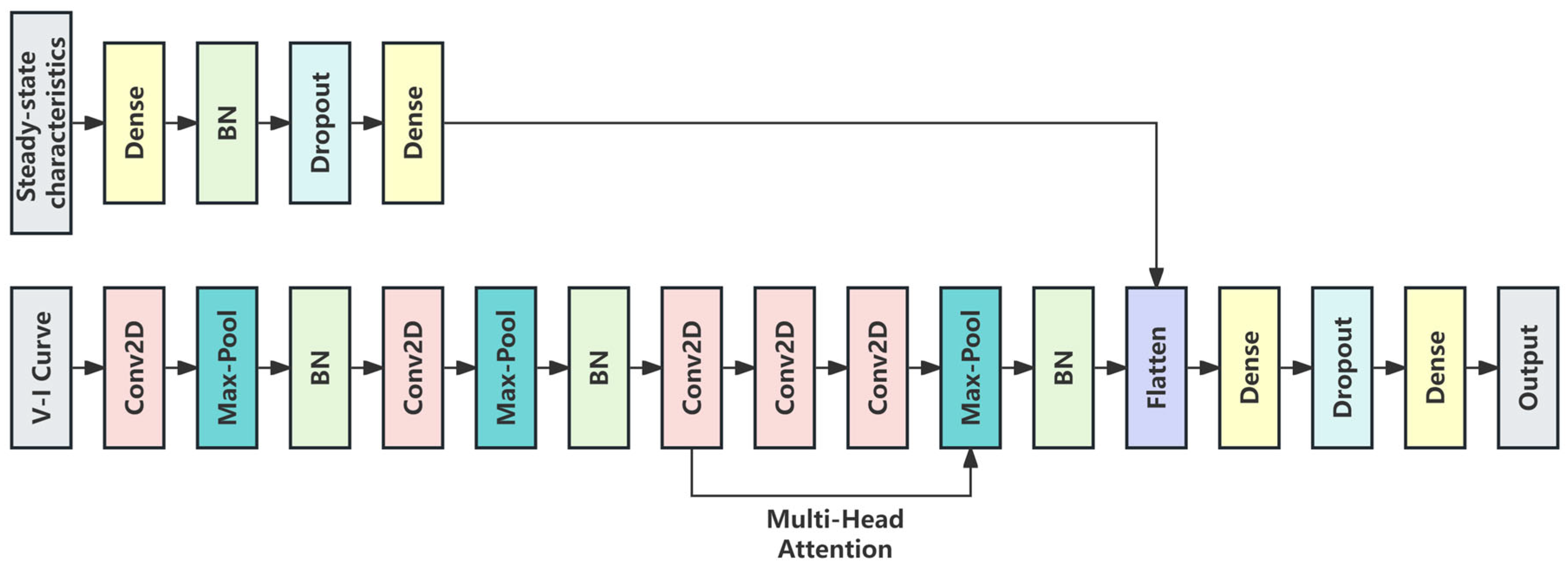
The load identification model proposed in this paper, which integrates stable state features and lightweight networks, adopts an end-to-end deep learning architecture and is implemented through a dual-branch network. It includes a lightweight V-I trajectory feature extraction branch and a stable state feature extraction branch. The electrical V-I trajectory image and stable state features are fused into the input of the dual-branch lightweight network, thereby more reliably estimating the probability of electrical appliance categories. The entire model can be divided into four clear and orderly modules: the input module, the feature extraction module, the fusion and classification module, and the output module. The overall structure flowchart of the model is shown in Figure 6.

2.2.1. Depthwise Separable Convolution

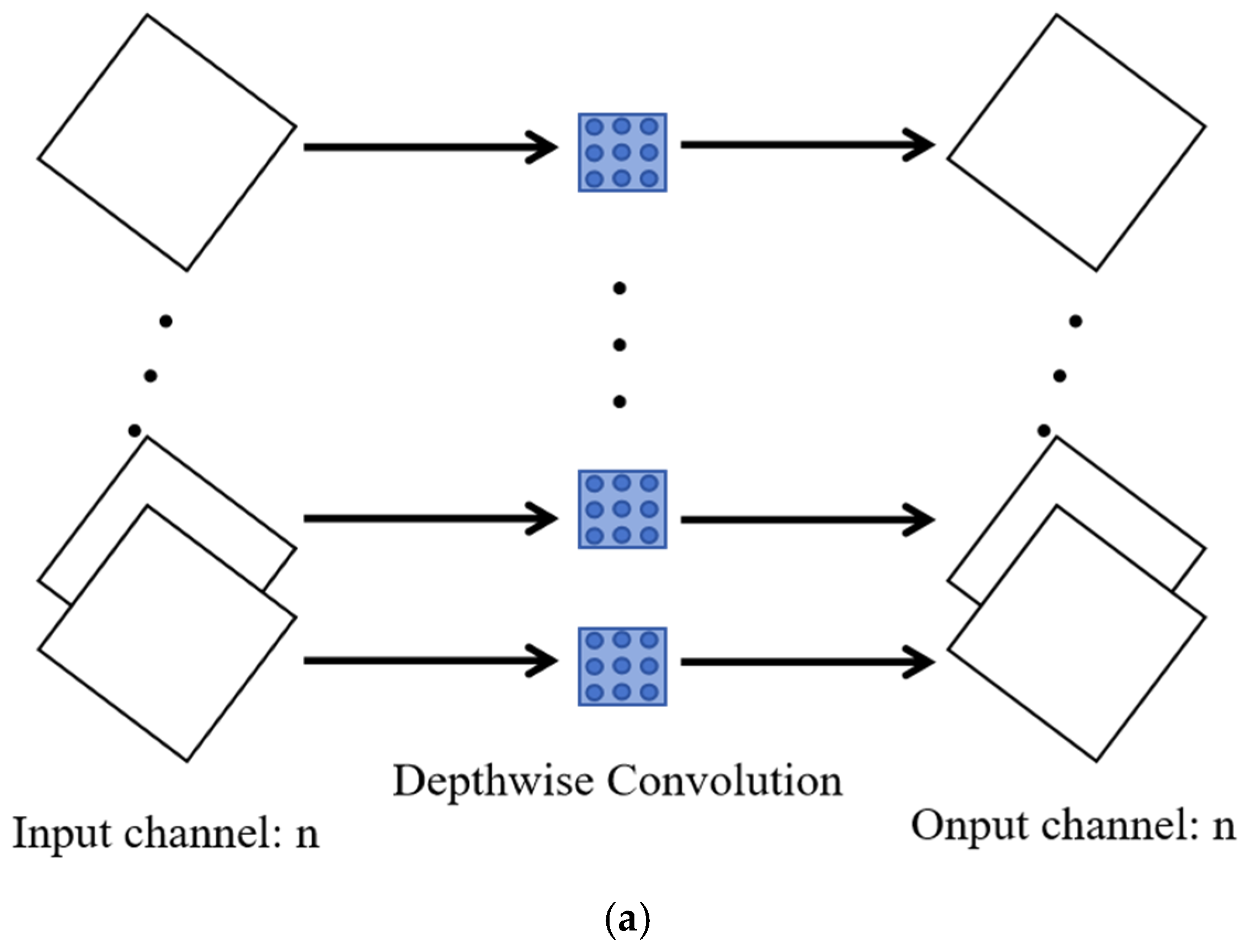
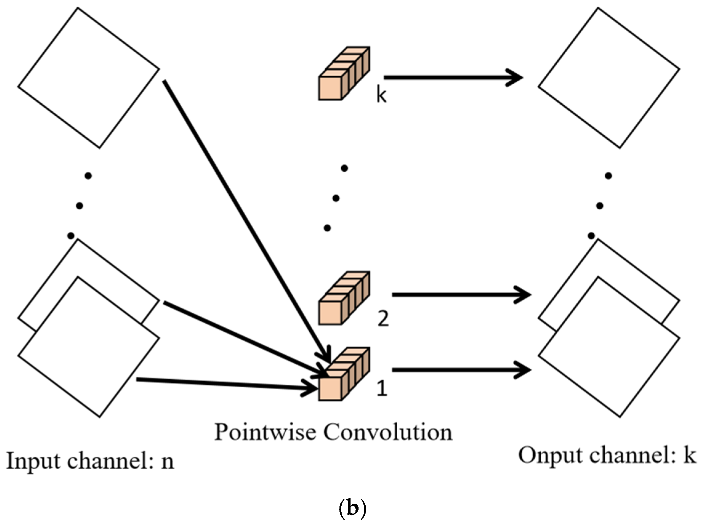
To ensure the feature extraction capability while reducing the model parameters and computational complexity, this paper adopts depthwise separable convolution (Depthwise Separable Convolution, DSC) to construct the convolution feature extraction module. Depthwise separable convolution decomposes the standard convolution into two independent steps: a depthwise convolution per channel and a pointwise convolution across channels, significantly reducing the parameter size and computational cost, making the model more suitable for edge deployment scenarios [38]. The specific internal structure is shown in Figure 7.
Given the input feature map X R H × W × C in , the standard convolution uses a four-dimensional convolution kernel W R K × K × C in × C out , to simultaneously complete spatial feature extraction and channel information fusion, and its parameter quantity is:
P std = K 2 C i n C o u t
And the depthwise separable convolution decomposes this process into two stages:
1.
Depthwise Convolution
Using C i n individual independent single-channel convolution kernels W dw R K × K × 1 × C in , each convolution kernel only acts on the corresponding input channel, and the number of output channels is the same as the number of input channels. As shown in Figure 7a, in this stage, only the spatial features of each channel are extracted, and there is no information interaction between channels. The parameter quantity of depthwise convolution is:
P d w = K 2 C i n
2.
Pointwise Convolution
Using C i n 1 × 1 convolution kernels W pw R 1 × 1 × C in × C out , as shown in Figure 7b, the output channels of the deep convolution are linearly combined to achieve information fusion and dimension transformation between channels. The parameter quantity of pointwise convolution is:
P p w = C i n C o u t
Therefore, the total number of parameters of the depthwise separable convolution is:
P d s = K 2 C i n + C i n C o u t
The ratio of the number of parameters to that of the standard convolution is:
P d s P s t d = K 2 C i n + C i n C o u t K 2 C i n C o u t = 1 C o u t + 1 K 2
Referring to Formula (17), for example, when the number of output channels C o u t is large and the convolution kernel size K = 3, the parameter quantity of the depthwise separable convolution is approximatel 1 9 of the standard convolution, significantly reducing the storage and computing requirements of the model.
As shown in Table 3, after applying depthwise separable convolution, the total number of parameters in the convolution feature extraction module decreased from 92,448 to 11,145, with a reduction rate of 87.9%. Correspondingly, the computational complexity decreased from O K 2 C i n C o u t H W to O K 2 + C o u t C i n H W , significantly improving the computing efficiency and greatly reducing the inference latency of the model on edge devices.

2.2.2. Convolutional Feature Extraction Module

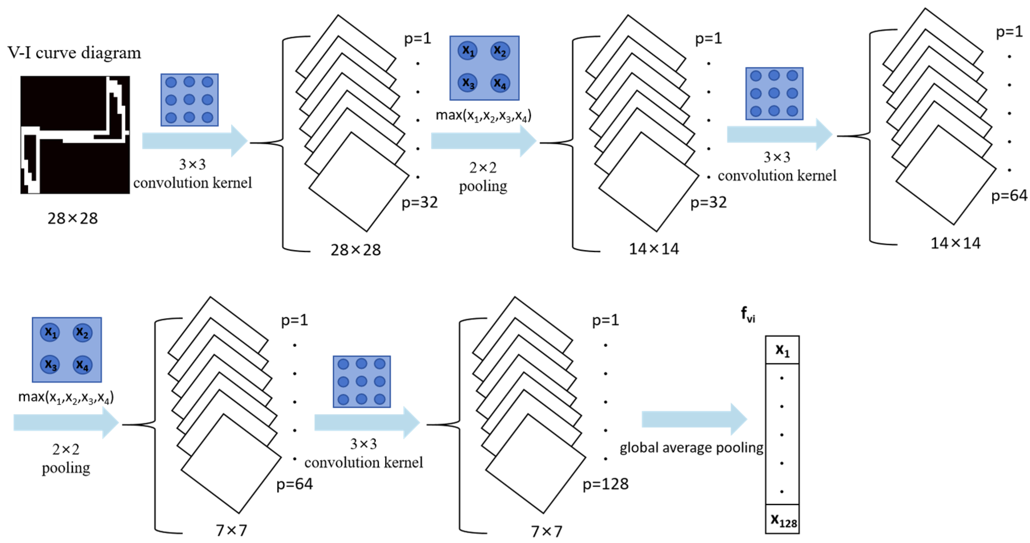
The convolution module employs a three-layer convolution structure to extract V-I trajectory features from the low-level to the high-level. Therefore, after each layer of convolution, batch normalization (Batch Normalization, BN) and ReLU activation functions are immediately applied. It is worth noting that batch normalization appropriately standardizes the activation values within each layer, which is conducive to accelerating convergence and has a slight regularization effect. The ReLU activation function is used to introduce the necessary nonlinearity. The specific process of the convolution feature extraction module is shown in Figure 8.
1.
First layer convolution
The first layer convolution is used to extract the low-level features of the V-I trajectory, including edges, directions and local textures:
F 1 d w = W d w 1 X v i ˜
F 1 = D r o p o u t 0.2 M a x P o o l B N R e L U W p w 1 F 1 d w + b 1
Among them:
W dw 1 R 3 × 3 × 1 × 1 : Deep convolutional kernel, with a size of 3 × 3, independent convolution per channel;
W pw 1 R 1 × 1 × 1 × 32 : Pointwise convolution kernel, maps a single-channel to 32 channels;
: Channel-wise depthwise convolution operation, with the number of groups equal to the number of input channels;
b 1 R 32 : Offset term;
MaxPool : 2 × 2 Maximum pooling with a stride of 2, and the output size is halved;
Dropout 0.2 : Randomly discard neurons with a probability of 0.2 to prevent overfitting.
The output feature map size is 14 × 32 × 32.
2.
Second Layer Convolution
Since the second layer convolution operates on the feature map after the first pooling, its receptive field is already quite large. Therefore, it naturally facilitates the detection of various local shapes such as arcs, straight lines, and turning points.
As the size of the output feature map selected is, the Dropout rate is appropriately increased to 0.3 to prevent overfitting that may occur when the feature dimension increases.
F 2 d w = W d w 2 F 1
F 2 = D r o p o u t 0.3 M a x P o o l B N R e L U W p w 2 F 2 d w + b 2
Among them, W dw 2 R 3 × 3 × 32 × 1 ,   W pw 2 R 1 × 1 × 32 × 64 , the output feature map size is 7 × 7 × 128. The dropout rate has been increased to 0.3 to address the overfitting risk caused by the increase in feature dimensions.
3.
Third Layer Convolution
The third layer of convolution no longer undergoes pooling, in order to retain spatial information for the use of the attention mechanism:
F 3 d w = W d w 3 F 2
F 3 = B N R e L U W p w 3 F 3 d w + b 3
Among them, W dw 3 R 3 × 3 × 64 × 1 , W pw 3 R 1 × 1 × 64 × 128 , the output feature map size is. At this point, the receptive field of each neuron has covered most of the area of the original image, and is capable of recognizing the overall trajectory shape features, such as elliptical, linear, and bowtie-shaped, etc.
After global average pooling, the V-I feature vector is obtained:
f v i = 1 H × W h = 1 H w = 1 W F 3 h , w R C
Here, H , W represents the size of the feature map, and C = 128 represents the number of channels.

2.2.3. Multi-Head Attention

In order to better extract the long-distance spatial dependency and global structural information in the V-I trajectory, this paper introduces the multi-head attention mechanism. Unlike the convolutional layers that only act on local neighborhoods, the attention mechanism can directly and precisely calculate the correlation between any two positions in the image. Therefore, it is very friendly to the symmetry and periodicity of the V-I trajectory.
1.
The basis of self-attention mechanism
The core of the self-attention mechanism is to calculate the correlation weights between each position in the sequence and other positions, and to enhance the feature representation through weighted aggregation. Given an input sequence, the self-attention calculation process is as follows:
(a) Linear transformation generates the query, key, and value matrices
Q = XW Q ,   K = XW K ,   V = XW V
Among them, W Q , W K , W V R d × d k are learnable weight matrices.
(b) Calculate the attention weights
The attention weight is calculated through the dot product of the query and the key, and then normalized by Softmax:
α ij = Softmax q i k j d k = exp q i k j d k l = 1 n exp q i k j d k
(c) Weighted Aggregation
Attention Q , K , V = softmax QK T d k V
2.
Multi-head Attention Mechanism Calculation
Since the multi-head attention mechanism uses several parallel attention heads to extract the correlations between features from different representation subspaces, it naturally enhances the expressive power of the model.
Definition: Let the number of attention heads be h, and the dimension of each head be d k = d / h . Then the multi-head attention is defined as:
MultiHead Q , K , V = Concat head 1 , head 2 , , head h W O
Among them, in this paper, we set h = 4 , then the dimension of each head d k = d / h = 32 , which means the sequence length L = 32 .
The calculation process of each attention head is as follows:
head i = Attention Q W i Q , K W i K , V W i V
Among them, Q , K , V all come from the same input sequence F seq (the self-attention mechanism), and W i Q , W i K , W i V are the learnable projection matrices for the first head.
3.
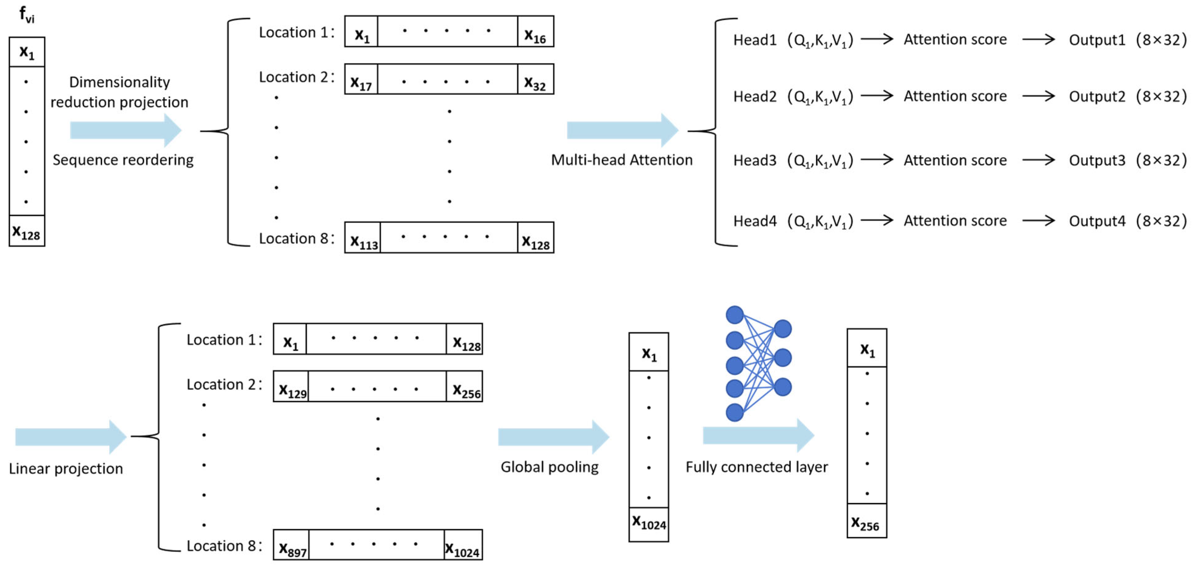
Lightweight Multi-head Attention Design
As shown in Figure 9, this paper has made a very effective lightweight design for the multi-head attention module required for edge deployment scenarios. The reason is that the multi-head attention mechanism in the standard Transformer is indeed beneficial for extracting long-range dependencies, but its computational complexity is O L 2 d + Ld 2 , where L is the sequence length and d is the feature dimension. Therefore, directly using the standard multi-head attention to process the V-I trajectory features ( d = 128 , L = d / h = 32 ) would have a significant computational cost.
Therefore, this paper elaborates on the following lightweight improvement methods for the discussion:
(a) Dimensionality Reduction Projection: Since the features have been reduced in dimension before the attention calculation, the computational complexity has been lowered:
Q = ReLU XW proj Q , K = ReLU XW proj K , V = ReLU XW proj V
Among them, W proj R d × d proj , d proj = 64 represents the reduced dimension. After dimension reduction, the complexity of attention calculation decreases from O L 2 d + Ld 2 to O L 2 d proj + Ld proj 2 .
Dimension reduction ratio: r = d proj / d = 64 / 128 = 0.5 means that the feature dimension is reduced by half, and theoretically, the computational load is reduced by approximately 75%.
(b) Feature reshaping: Since the V-I features extracted by the convolutional neural network are in vector form f vi R 128 , and the attention mechanism requires the input to be in sequence form x 1 , x 2 , , x L R L × d model , this paper reasonably designs a feature reshaping module to convert the vector features into sequence features:
X seq = Reshape f vi R L × d model
Here, L = d proj / h = 16 represents the sequence length, N seq = 8 represents the number of sequences, and d model = 128 represents the model dimension.
Since this design enables each position of the sequence to naturally and fully learn the feature representations of each region of the V-I trajectory, it provides a reasonable input structure for the attention mechanism.
(c) Multi-head Attention Calculation: The calculation process is consistent with the previous one. To alleviate the problem of gradient vanishing in deep networks and accelerate the training convergence, residual connections and layer normalization are added after each attention sub-layer:
Z = LayerNorm X seq + MultiHead X seq
(d) Feedforward Network
To enhance the model’s nonlinear expression ability, a feedforward network (FFN) is added after the attention layer:
FFN x = GELU xW 1 + b 1 W 2 + b 2
Among them, W 1 R d model × 4 d model ,   W 2 R 4 d model × d model , the definition of the GELU activation function is:
GELU x = x Φ x = x 1 2 1 + erf x 2
Ultimately, the output of the entire attention module is:
Z out = LayerNorm Z + FFN Z

2.2.4. Other Steady-State Feature Extraction Module

The steady-state characteristics include power characteristics and geometric characteristics of the V-I curve. The power characteristics include active power P and reactive power Q . The digital characteristics of the V-I curve include the area A of the curve and the slope β of the middle section. Together with the power characteristics, they form the steady-state feature vector. Correspondingly, the steady-state feature encoding network adopts a three-layer fully connected structure. Its design concept is very clear: the shallow layer performs nonlinear transformation, and the deep layer obtains the feature representation.
1.
First layer: Feature expansion
h 1 = ReLU W p 1 P , Q , A , β + b p 1
Here, P , Q , A , β R 4 represents the input, W p 1 R 4 × 32 ,   b p 1 R 32 . This layer expands the 4-dimensional steady-state features to 32 dimensions, thereby enhancing the feature expression capability.
2.
Second layer: Batch normalization and activation
h 2 = Dropout BatchNorm h 1 , p = 0.2
The calculation formula for batch normalization is:
BatchNorm h = γ h μ B σ B 2 + ϵ + β
Among them, μ B and σ B 2 represent the mean and variance of the current batch of data, and γ and β are learnable parameters.
3.
Third layer: Feature compression
f steady = ReLU W p 2 h 2 + b p 2 R 64
Among them, W p 2 R 32 × 64 . This layer further expands the 32-dimensional features to 64 dimensions, and matches them with the V-I features (256 dimensions) in terms of dimensions.

2.2.5. Feature Fusion and Model Training Strategies

1.
Feature Fusion and Classification
Combine and fuse the V-I characteristics with the power characteristics after enhancing the attention, as follows:
f fusion = Concat f vi attn , f steady R 256 + 64 = R 320
Here, f vi attn = Flatten Zout R 256 .
The fused features are classified through two layers of fully connected networks, as follows:
h c 1 = ReLU W c 1 f fusion + b c 1
h c 2 = Dropout BatchNorm h c 1
The final output category probability is as follows:
y ^ = Softmax W c 2 h c 2 + b c 2 R C
Here, C = 11 represents the number of electrical appliance categories.
2.
Model Training Strategy
This paper employs sparse categorical crossentropy as the loss function. Unlike the standard categorical crossentropy, the sparse version requires the labels to be integer indices rather than one-hot encoding, which is more suitable for multi-classification tasks and saves memory:
L CE = 1 N i = 1 N log y ^ i , y i
Among them are the following:
N : Batch size;
y i : The true label of the nth sample (an integer, within the range of 0 , 1 , , K 1 );
y ^ i , y i : The probability that the model predicts the ith sample belongs to the true category y i .
This loss function encourages the model to assign a high probability to the true category and a low probability to the incorrect category. When the prediction is completely accurate, L CE = 0 . The less accurate the prediction is, the larger the loss value will be.
After incorporating L2 regularization, the total loss during model training is:
L = L CE + λ l = 1 L W l 2 2
Since this paper uses the Adam optimizer (Adaptive Moment Estimation) for parameter updates, it combines the momentum method and the adaptive learning rate method very well. Thus, it can adaptively adjust the learning rate according to the historical gradient of each parameter, resulting in a fast convergence speed and being very robust to hyperparameters.
The parameter update rule is as follows:
m t = β 1 m t 1 + 1 β 1 θ L t
vt = β 2 v t 1 + 1 β 2 θ L t 2
m ^ t = m t 1 β 1 t , v ^ t = v t 1 β 2 t
θ t + 1 = θ t η m ^ t v ^ t + ϵ
Among them:
η = 0.001 : Initial learning rate;
β 1 = 0.9 : First-order moment decay rate;
β 2 = 0.999 : Second-order moment decay rate;
ϵ = 10 7 : Numerical stability constant.
To accelerate the convergence of training and improve the final performance, an exponential decay learning rate scheduling strategy is adopted:
η t = η 0 γ t / step
Among them:
η 0 = 0.001 : Initial learning rate;
γ = 0.9 : Decay rate;
step   =   100 : Decay step size (decreases every 100 iterations);
: Floor function.
This scheduling strategy causes the learning rate to be reduced to 96% of its original value every 100 steps. It maintains a relatively high learning rate in the early training stage for rapid convergence, and reduces the learning rate in the later stage for fine-tuning.
To prevent overfitting, the early stopping mechanism is adopted. Training is stopped when the validation set loss does not improve for p consecutive rounds, and the model weights with the minimum validation set loss are restored.
stop = 1 min e epochs L val e   No   update   for   p   consecutive   rounds
This paper sets p = 30 , meaning the patience value (patience) is 30 rounds. This setting provides the model with sufficient exploration space while avoiding the loss of performance due to premature stopping.
Table 4 summarizes the main hyperparameters for model training.

3. Results

This chapter verifies the lightweighting effect of the model proposed in this paper and the superiority of using fused steady-state features from two aspects: contrast experiments and ablation experiments. Firstly, through two dimensions of performance analysis of the lightweight model alone and multi-model comparison experiments, combined with experimental results such as confusion matrices, accuracy-parameter quantity comparison, F1 score comparison, and training process curves, the effectiveness and engineering application value of the proposed lightweight dual-branch CNN model are comprehensively verified.

3.1. Contrast Experiment

3.1.1. Environmental Setup for Contrast Experiment

This experimental work is implemented based on Python 3.9 and TensorFlow 2.15 deep learning framework. The hardware environment used is: Intel Core i9-12900 K processor, 32 GB memory, and NVIDIA RTX 3090 graphics card. It is also noted that all the tested models use the same dataset division method, training strategy and hyperparameters, except for the medium CNN which made reasonable adjustments to the learning rate and batch size.

3.1.2. Performance Analysis of Lightweight Dual-Branch CNN Model Alone

1.
Analysis of Confusion Matrix for Lightweight Models
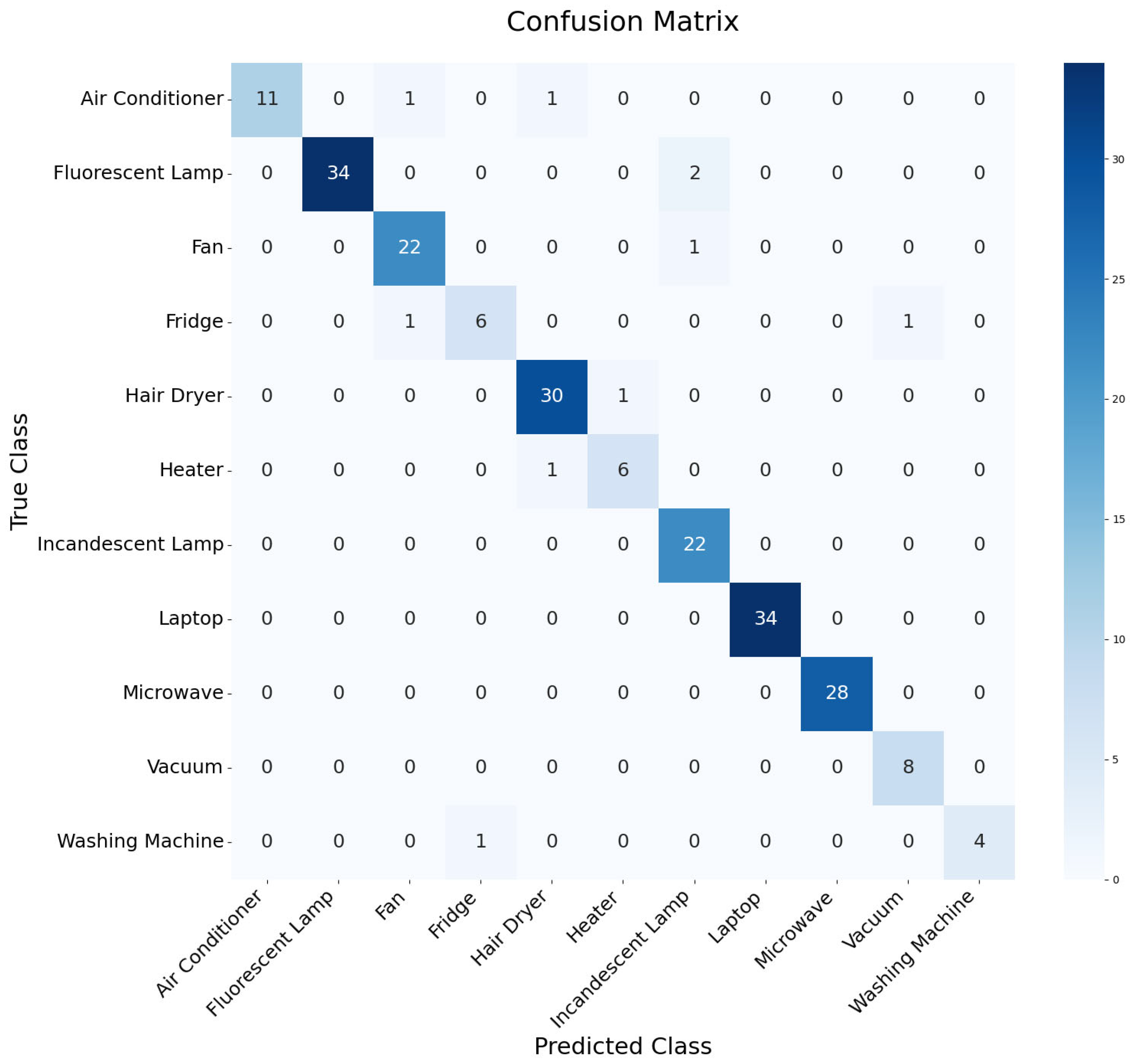
Figure 10 shows the confusion matrix of the lightweight dual-branch CNN model proposed in this paper, which visually presents the classification performance of the model on 11 types of household appliances.
From the confusion matrix in Figure 10, the following conclusions can be drawn:
High-identification appliances achieved nearly perfect identification. Therefore, it can be clearly seen from fluorescent lamps (34/36), hair dryers (30/31), laptops (34/34), microwave (28/28), vacuum (8/8), etc. that the correct classification values along the diagonal are much higher than the misclassification values. Thus, it can be concluded that the model has a strong discriminatory ability for load features that are obviously V-I trajectory and power characteristics stable.
The model demonstrates excellent identification performance for appliances with moderate distinguishability: the existing results clearly show that the fan (22/23) and incandescent lamp (22/24) were misclassified only once and twice, respectively, thus clearly demonstrating the model’s ability to identify common household loads.
Low-identification appliances classification performance: The correct classification rates of air conditioners (11/13), heaters (6/7), and washing machines (4/5) are 84.62%, 85.71%, and 80.00% respectively. This also well illustrates that the model still has strong discrimination ability for multi-state loads with similar features.
Analysis of classification difficulties and reasons: Refrigerators are the weak point of the model’s classification performance. Among the 8 test samples, only 6 were correctly classified, with a correct classification rate of 75.00%. The main reasons include:
(a) The sample size for refrigerators is the smallest, and the imbalance of data may lead to insufficient model learning;
(b) Refrigerators have periodic start-stop loads, and the V-I trajectory has local similarities with some inductive loads;
(c) The fluctuation range of steady-state power characteristics is small, and the difficulty of feature distinction is higher than that of linear loads and switch-type loads.
Model generalization ability verification: The non-diagonal misjudgment values in the overall confusion matrix are very few, there is no obvious class bias, indicating that the model has balanced learning in all classes, excellent generalization ability, and no category-specific deviation caused by overfitting.
2.
Stability Analysis of Lightweight Model Training
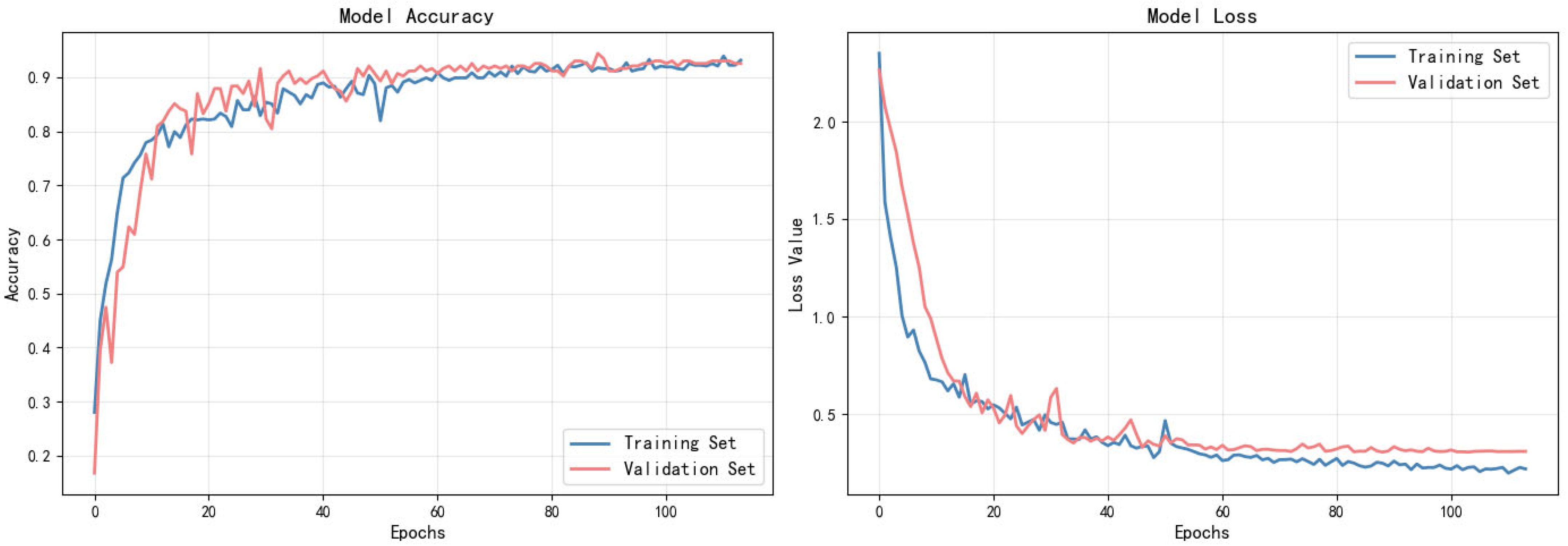
Figure 11 shows the training process curve of the lightweight CNN, including the changes in accuracy and loss values of the training set/verification set.
From the training curve, it can be seen that:
(1) The convergence speed is fast: The model converges rapidly within 30 rounds, the accuracy on the validation set exceeds 90%, the loss rapidly drops below 0.5, and gradually converges and stabilizes between 50 and 80 rounds;
(2) The generalization control effect is good: The training and validation curves are overall consistent, the accuracy on the validation set does not decline, only a slight separation exists in the later stage, and the regular modules such as Dropout effectively constrain overfitting;
(3) The training is robust: The oscillation amplitude of the later curve is limited, the validation accuracy remains stable at over 93%, the loss converges smoothly, the model training is sufficient, and the generalization ability is reliable.

3.1.3. Multi-Model Contrast Experiment Analysis

This paper focuses on developing a lightweight CNN model with extreme efficiency as its core design principle. It eliminates the batch normalization layer to reduce computational costs and adopts a three-level lightweight convolution structure to complete V-I feature extraction. It replaces the traditional flattening layer and redundant fully connected layer with global average pooling, significantly compressing the model’s parameter quantity. Combined with other stable feature enhancement, it has the advantages of fast inference speed and low deployment cost, and is suitable for edge deployment scenarios.
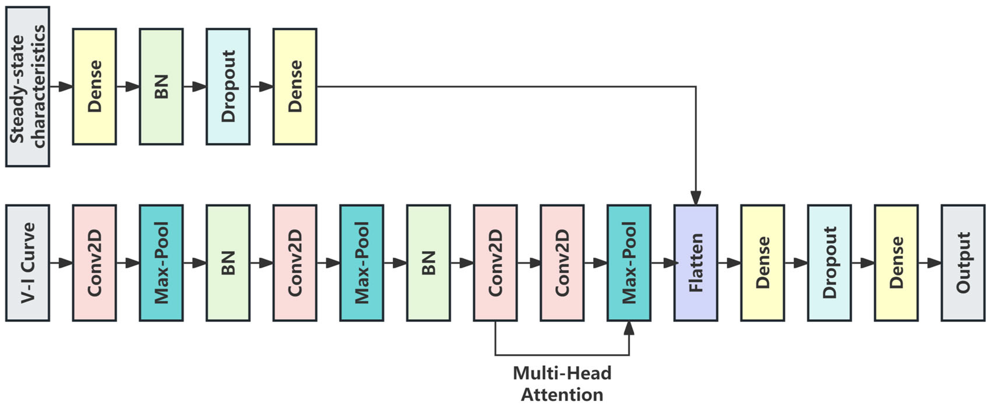
To verify the effectiveness of the lightweight model, this paper sets standard CNN and medium CNN as the comparison experimental objects. To control the variables, both are also set as dual-branch networks with additional steady-state feature branches. Among them, standard CNN is a traditional deep and large-capacity network, which enhances the feature extraction ability by stacking five-level convolution modules and configuring batch normalization layers layer by layer, and sets two layers of 4096-dimensional fully connected layers to fit high-dimensional feature information; medium CNN also simplifies the convolutional layers of the standard model, controls the number of network parameters, optimizes the arrangement position of batch normalization layers, but does not introduce methods such as depthwise separable convolution and lightweight attention mechanism to reduce the number of parameters. The specific structures of the two comparison models are shown in Figure 12 and Figure 13.
3.
Comparison of Confusion Matrices
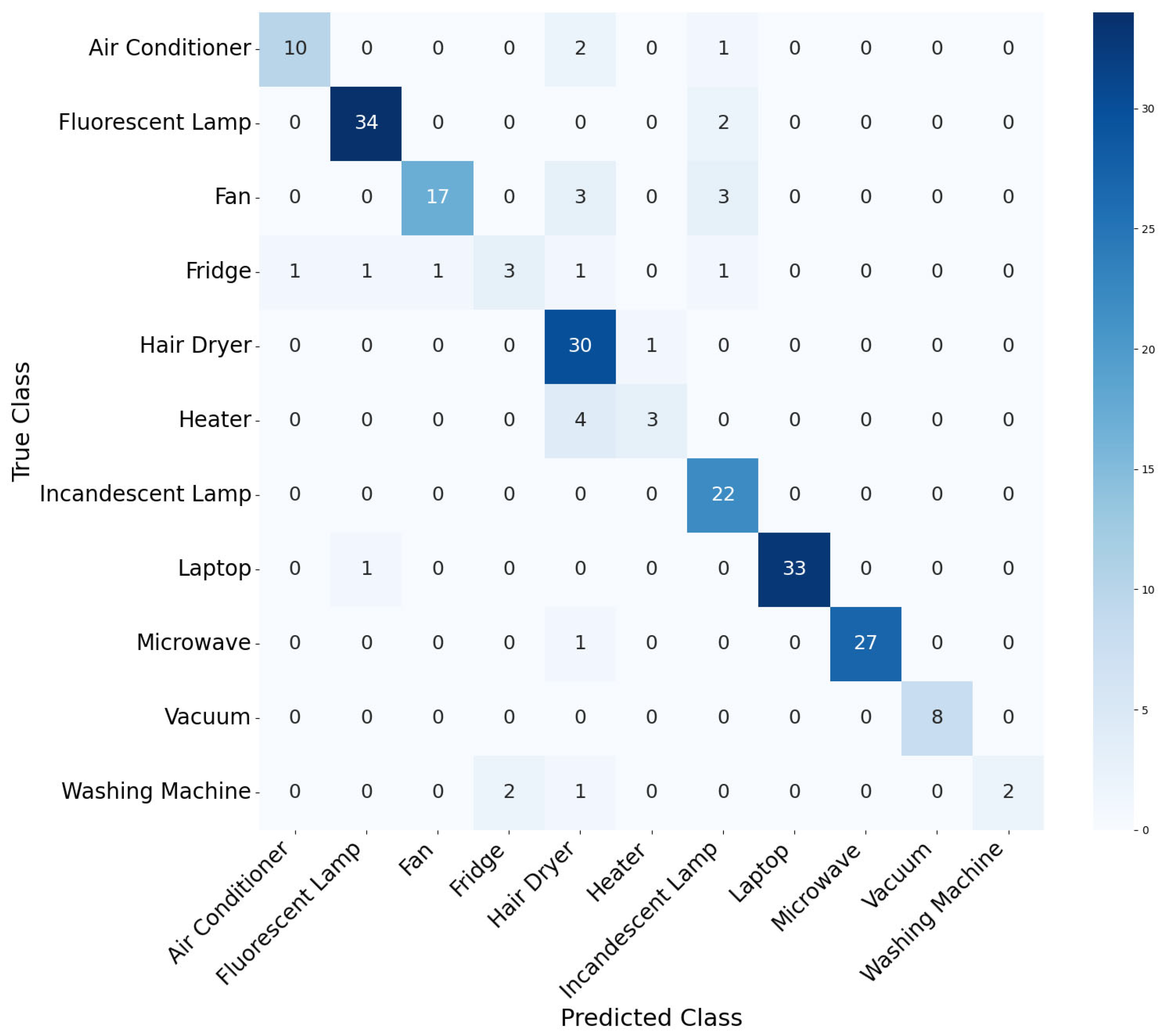
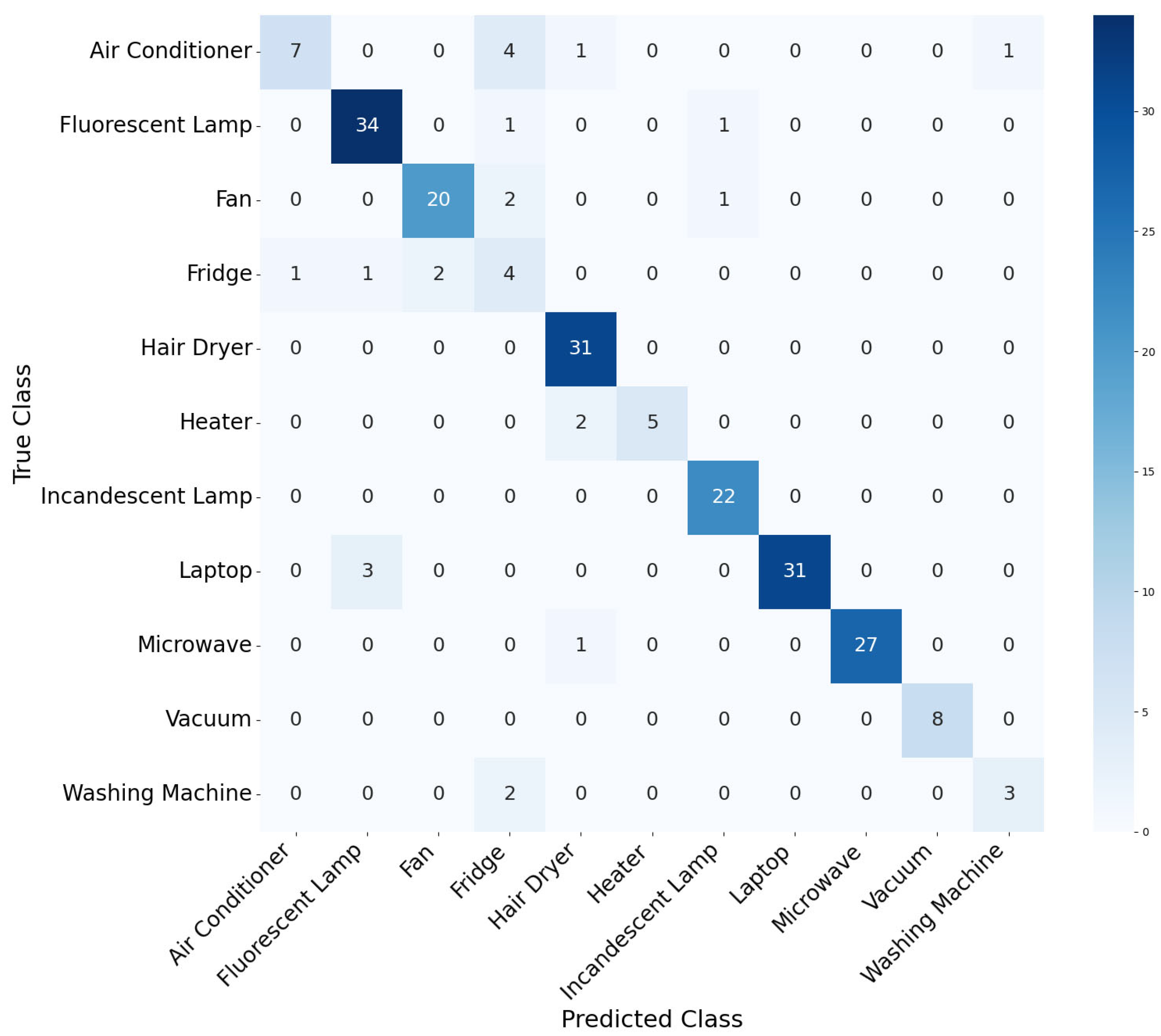
Figure 14 and Figure 15 respectively show the confusion matrices of the standard CNN and the medium CNN, and a horizontal comparison is made with the lightweight CNN.
From the comparison of the confusion matrices of the three different models in Figure 10, Figure 14 and Figure 15, the following conclusions can be drawn:
The three models perform relatively consistently in the identification of high-visibility electrical appliances. The three models achieve extremely high correct classification rates for appliances with significant feature differences, such as fluorescent lamps, hair dryers, laptops, microwave ovens, and vacuum cleaners, indicating that the identification difficulty of this type of load is low, and all three models can effectively extract their features.
The identification performance of the three types of models varies significantly on low-visibility appliances. Appliances with similar characteristics such as air conditioners, heaters, and refrigerators are difficult to classify: the standard CNN has a relatively high misclassification rate for air conditioners and heaters; while the medium CNN, through structural optimization, significantly reduces the misclassification rate of heaters and significantly improves the identification accuracy of air conditioners.
The lightweight CNN model performs the best in the identification of low-visibility appliances. The identification of air conditioners and heaters by all three models is the best among the three models, verifying the advantages of lightweight models and global average pooling in extracting features of fine classification categories.
The lightweight model has significantly fewer misjudgments in small sample categories such as refrigerators and washing machines compared to the standard CNN. Therefore, it can be proven that this model has a better learning effect for small sample and low-contrast categories.
4.
Comprehensive Comparison of Model Performance
Table 5 presents the comparison results of the parameter quantities of the three models and the various evaluation indicators of each model.
From the results, the following core conclusions can be drawn:
The lightweight CNN proposed in this paper, with only 0.17M parameters, has achieved a test accuracy of 95.35%, which is higher than that of the standard CNN (87.91%) and the medium CNN (89.30%). Therefore, the effectiveness of the lightweight design in this paper has been fully demonstrated.
The medium CNN achieves an effective compromise between accuracy and parameters: the optimized medium CNN has 1.84M parameters, with an accuracy rate of 89.30%, which is 1.39 percentage points higher than the standard CNN and 0.30 percentage points higher than the optimized medium CNN. This proves the gain effect of structural optimization on medium-sized models.
Since the parameter quantity of the standard CNN is 38.31M, which is 225 times that of the lightweight CNN, and its accuracy rate is the lowest, it can be concluded that the traditional CNN with large parameter quantity has a performance bottleneck in the non-intrusive load identification task and is not suitable for edge deployment.
The lightweight CNN is also in the leading position in two indicators of macro average F1 (92.73%) and weighted average F1 (95.31%). Therefore, it can be concluded that the lightweight model is more balanced in learning for various categories and has better generalization ability for small sample and ambiguous loads.
The macro average F1 score of the medium-sized CNN model was 83.52%, which was much lower than that of the lightweight CNN. This indicates that the medium-sized model still has significant class bias. The generalization ability of the standard CNN is limited: although the weighted F1 has reached 87.31%, the macro average F1 is only 80.34%. This can lead to the conclusion that the model relies on large sample classes for performance and has poor generalization ability for small sample classes.
5.
Comparison Analysis of F1 Scores for Various Categories
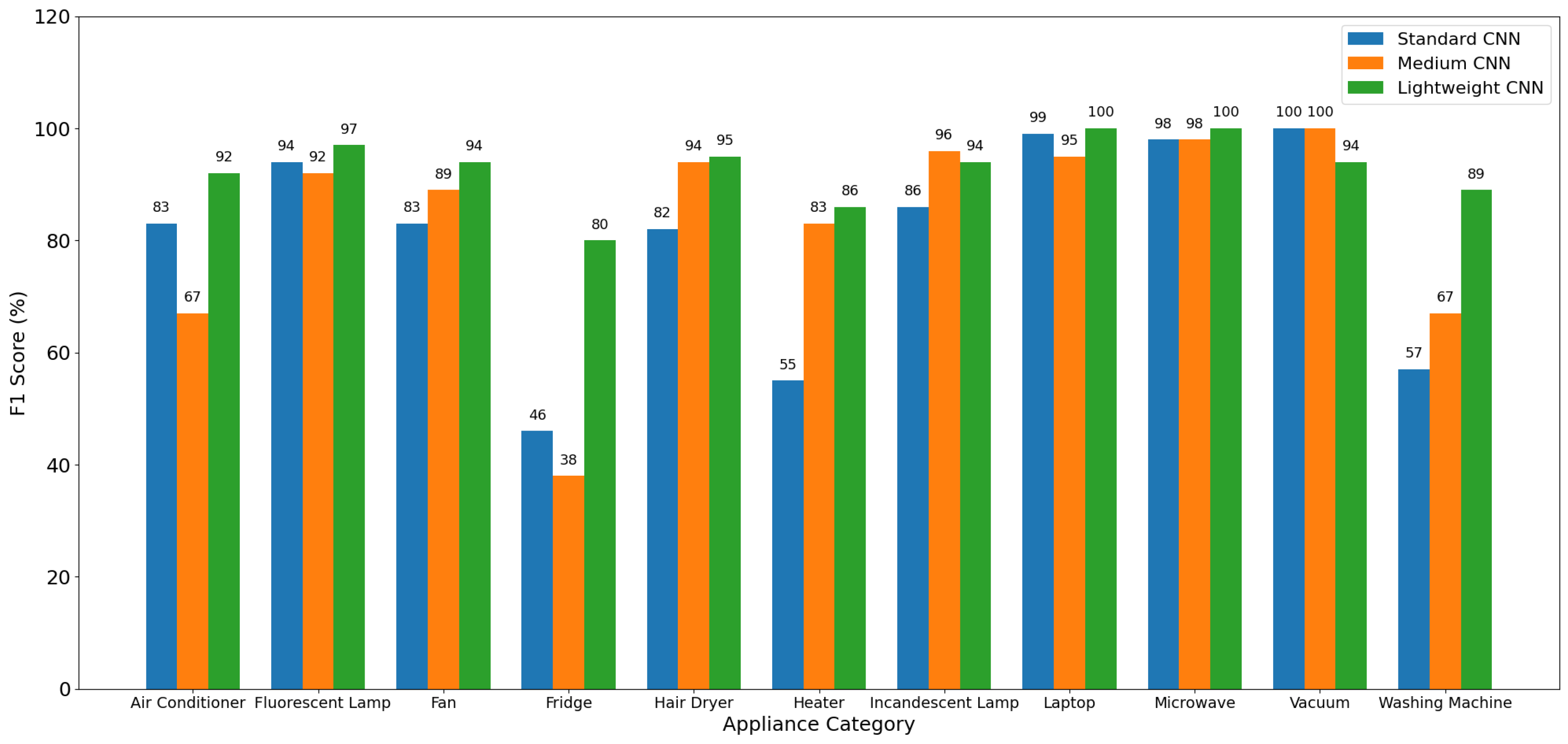
Figure 16 shows the F1 score comparison results of the three models on 11 types of electrical appliances, further quantifying the performance differences of the models on individual categories.
From Figure 16, the following conclusions can be drawn:
Except for the three categories of notebook, microwave oven, and vacuum cleaner, where the F1 scores of the three models were all nearly 100%, the lightweight CNN performed the best in most other categories. Especially in categories such as air conditioner (92%), fridge (80%), and washing machine (89%), where there are many similar items, the lightweight CNN outperformed the standard CNN and medium CNN. It also provided excellent improvement for small sample and multi-state load conditions.
The performance of the medium CNN significantly decreased in the recognition of various appliances such as fridge (38%), washing machine (67%), and air conditioner (67%). Therefore, it can be concluded that when its structure is unreasonable, it is prone to underfitting and the features are not adequately learned. The standard CNN has obvious shortcomings: due to the low F1 scores measured in categories such as air conditioner, fan, and fridge, the overall accuracy of all types is currently limited, and redundant parameters have not brought performance improvement.
6.
Advantages of Lightweight Models and Engineering Application Value
The lightweight CNN model proposed in this paper achieves the unity of extreme lightening and high accuracy by replacing the traditional fully connected layer with global average pooling, simplifying convolutional channels, and optimizing the dual-branch feature fusion structure:
With a parameter quantity of only 0.17M, the test accuracy reached 95.35%, which was 7.44 percentage points higher than that of the standard CNN and 6.05 percentage points higher than that of the medium CNN.
Since the parameters and computational volume of the model are extremely small, it is naturally suitable for real-time operation on embedded devices (STM32, Raspberry Pi), so there is no need to rely on cloud servers, which reduces deployment costs and communication latency.

3.2. Ablation Experiment

3.2.1. Environmental Setup for Ablation Experiment

To verify the effectiveness of the fusion of steady-state features in the dual-branch lightweight neural network model proposed in this paper, this paper conducted an ablation experiment on the PLAID public dataset. In the experiment, two different structures of models were compared:
  • Single-branch model (only V-I trajectory): Using only the V-I trajectory as the input feature;
  • Dual-branch model (V-I trajectory + other steady-state features): Fusing other steady-state features on the basis of the V-I trajectory.
To strictly isolate the contribution of steady-state features, the single-branch comparison model adopts the identical lightweight backbone: three-layer depthwise separable convolution and lightweight multi-head attention, only removing the steady-state feature branch and corresponding fully connected encoding network. All training hyperparameters, image preprocessing methods remain completely consistent with the dual-branch model, eliminating the interference of network structure differences on accuracy gain. The accuracy rate, Macro F1 and Weighted F1 were selected as evaluation indicators. The selected model was trained using the Adam optimizer, with an initial learning rate of 0.001, a batch size of 32, a maximum training round of 100, and an early stopping mechanism to control overfitting.

3.2.2. Comparison of Model Performance of Single-Branch and Dual-Branch Models

1.
Overall Performance Comparison
The overall performance comparison of the two models on the PLAID dataset is shown in Table 6.
From the results in Table 6, it can be seen that the dual-branch model outperforms the single-branch model in all evaluation indicators. Specifically, the accuracy of the dual-branch model is 95.3%, which is 11.6 percentage points higher than that of the single-branch model (83.7%). The macro average F1 score is 92.7%, which is 18.1 percentage points higher than that of the single-branch model (74.6%). The weighted F1 score is 95.3%, which is 12 percentage points higher than that of the single-branch model (83.3%). Therefore, it can be concluded that incorporating multi-modal feature fusion is beneficial for improving the performance of load identification.
2.
Analysis of Performance in Various Categories
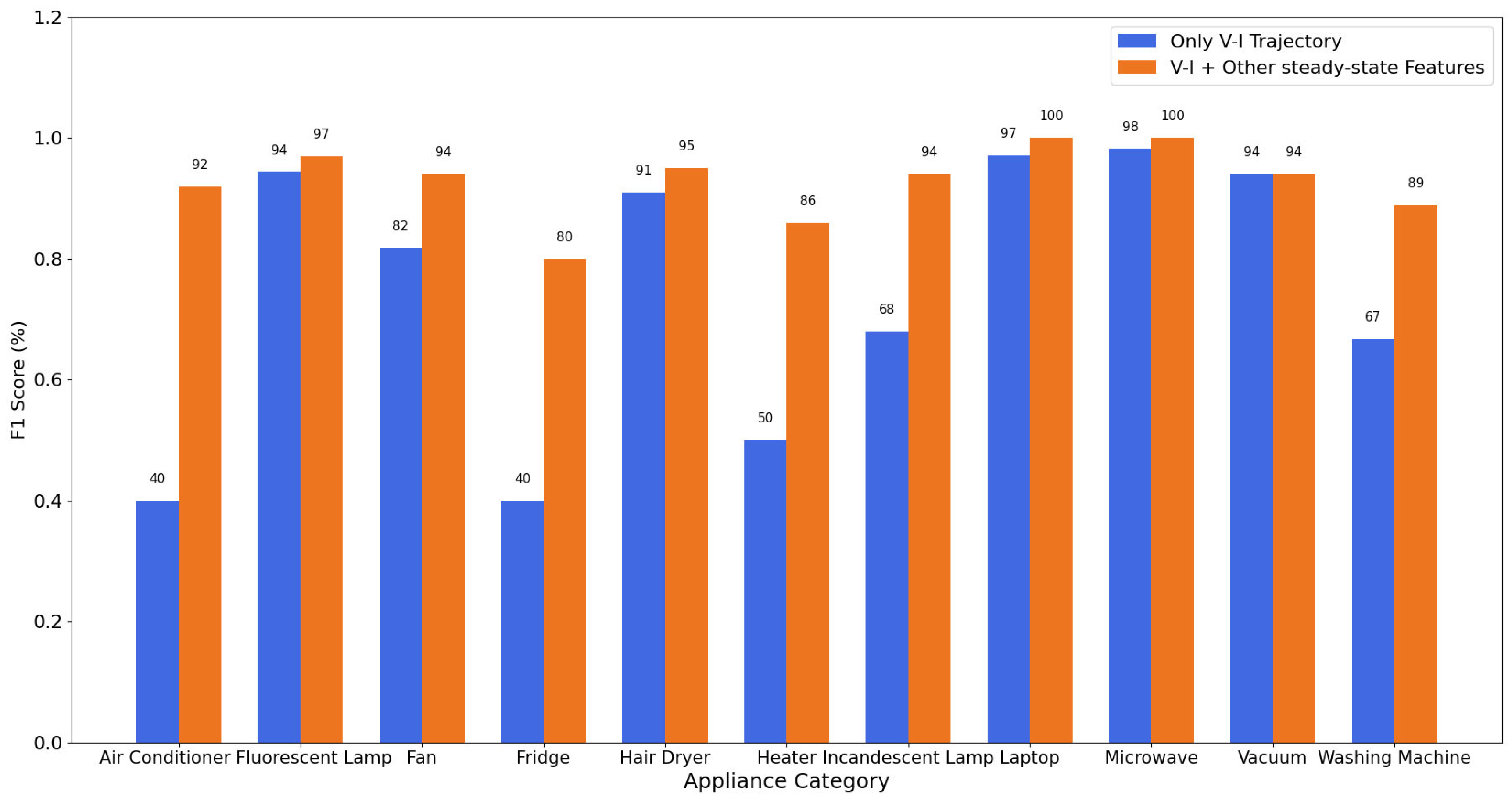
To further analyze the impact of power characteristics on the identification effect of different types of electrical appliances, Figure 17 presents a comparison of F1 scores for the two models across various categories. From this, it is clearly evident that:
(a) Significant improvement category: From the current analysis, it is clearly observable that the F1 scores of high-power appliances such as air conditioners, fridges, and washing machines have shown a significant improvement. The reason is that the power characteristics of these appliances are very stable, allowing for reliable differentiation of their various operating states. Therefore, the introduction of other steady-state features has a beneficial promoting effect on the identification results.
(b) Steady improvement category: Since the F1 scores of various appliances such as fans, incandescent lamps, and washing machines have all increased within the range of 12% to 26%, it can be concluded that on the basis of the existing identification ability of the V-I trajectory characteristics of the studied appliances, the power characteristics play a supplementary and improving role.
(c) Basically unchanged category: Since the F1 scores of various appliances such as fluorescent lamps, hair dryers, laptops, microwaves, and vacuums are all at a relatively high level (above 90%), the dual-branch model has slightly improved or remained unchanged on the original basis. This indicates that for the appliance categories with relatively significant V-I trajectory characteristics, the marginal contribution of other steady-state characteristics is relatively limited, but it will not harm the performance.
3.
Confusion Matrix Analysis
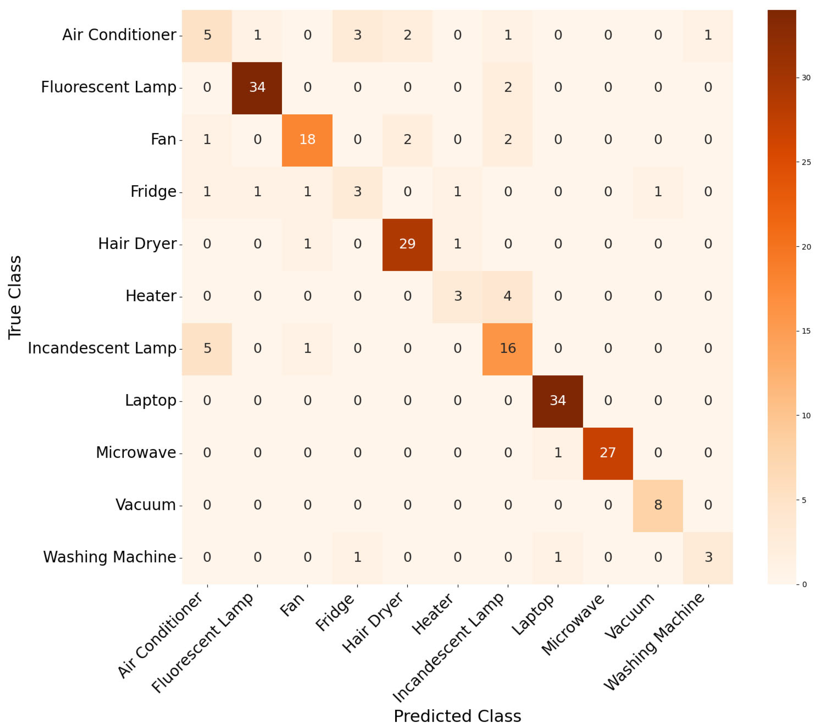
Figure 10 and Figure 18 present the normalized confusion matrices of the two models on the test set. By comparing them, it can be seen that:
(a) Due to the single-branch model (Figure 14), there are obvious confusion issues in all categories. For example, in the air conditioner category, there are five samples misclassified as incandescent lamps, one misclassified as a fan, and three misclassified as an air conditioner in the fridge category, and 1 misclassified as a washing machine. The fundamental reason for these misclassifications is that the various electrical appliances have highly similar V-I trajectory shapes.
(b) Due to the fact that the confusion matrix obtained by the dual-branch model (Figure 10) has concentrated diagonal elements, it is clearly visible that the recognition accuracy of each major category has exceeded 90%. Specifically, the recognition accuracy of air conditioners has increased from 38% to 85%, and the recognition accuracy of fridges has increased from 38% to 75%. Therefore, it can be reasonably assumed that the other steady-state feature branches have compensated for the deficiencies of the V-I trajectory features in this issue.

4. Discussion

4.1. The Advantages of This Model

4.1.1. Advantages of Lightweight Model in Edge Deployment

Under a unified hardware testing environment, we quantitatively demonstrated the deployment advantages of the dual-branch lightweight CNN proposed in this paper for edge terminals such as smart meters and low-power single-chip microcontrollers from two dimensions: model memory occupation and inference real-time performance. The specific comparison indicators are shown in Table 7.
The proposed model only contains 0.17M parameters, merely 1/225 of standard CNN and 1/11 of medium CNN. Stored in 32-bit float format, it occupies only 0.68 MB storage, while standard CNN takes over 153 MB and medium CNN occupies 7.36 MB. Smart meters and low-power MCUs are equipped with limited Flash/RAM; the two comparative models easily trigger memory overflow, yet our model can be deployed without storage expansion hardware.
Such extreme parameter compression benefits from depthwise separable convolution, which cuts convolutional parameters by 87.9%, together with global average pooling, channel compression and lightweight multi-head attention. These designs retain complete V-I trajectory feature extraction while shrinking model size drastically.
In terms of speed, our model achieves a single-sample batch latency of 0.5229 ms, 68.6% faster than standard CNN and 30.7% faster than medium CNN, with an average total inference time of only 49.896 ms. The 30 kHz sampling NILM system requires load classification within tens of milliseconds to support real-time demand response. The ultra-low latency reserves sufficient time for V-I trajectory generation and steady-state feature calculation on embedded chips, satisfying real-time monitoring of appliance switching events.
Depthwise separable convolution reduces computational complexity by splitting standard convolution into depthwise and pointwise operations. Lightweight multi-head attention lowers calculation cost by 75% via dimension projection, and the dual-branch parallel structure avoids redundant feature computation, jointly cutting floating-point operations during inference.

4.1.2. Comparison of Lightweight Models with Other Models

To verify the comprehensive performance of the dual-branch lightweight CNN model proposed in this paper, three representative cutting-edge literature models were selected for a horizontal comparison. The network structures, parameter quantities, and accuracy indicators of each model are shown in Table 8.
Compared with the three types of comparison models, the parameters of this model have been significantly reduced: compared with the traditional standard CNN, it is compressed by 99.2%; compared with ShuffleNetV2, it is compressed by 99.8%; compared with the lightweight network in reference [38], it is compressed by 84.1%. Relying on optimization methods such as depthwise separable convolution, lightweight multi-head attention, and global average pooling, while significantly reducing the floating-point operation volume, the feature extraction ability is retained. It can be directly deployed on ordinary smart meters, low-cost MCUs and other edge terminals, without the need for high-end computing hardware support, solving the pain points of existing models with excessive storage and computing power requirements, and being able to perform computations only on the cloud. The inference speed is also optimized simultaneously, with a single sample inference time of only 0.52 ms, meeting the real-time load identification requirements at 30 kHz high-frequency sampling.
In terms of accuracy, reference [30] only uses single-branch V-I image features, and similar appliances are easily confused, resulting in an identification accuracy of only 77.6%; reference [42] although builds multi-channel RGB images, still belongs to a single image modality, lacking numerical steady-state features for assistance. This paper adopts a dual-branch parallel structure, with one branch extracting spatial features of V-I trajectory images, and the other integrating active power, reactive power, trajectory geometric multi-dimensional steady-state features. The ablation experiments show that multi-feature fusion can improve the identification accuracy by more than 11%, significantly improving the classification effect for small sample and similar load features, effectively compensating for the deficiency of insufficient identification accuracy of a single V-I feature.
The identification accuracy of this paper is 95.35%, slightly lower than those of references [38,42], but the parameter quantity has been significantly reduced, and the comprehensive engineering value is better. Compared with the main comparison model in reference [38], the lightweight model of this paper only loses about 3% of the accuracy, but compresses the model parameters to 1/6 of the original, significantly reducing the cost of electric meter hardware transformation, and is suitable for large-scale implementation in the power grid.

4.2. Limitations of This Model and Potential Challenges

4.2.1. Limitations of This Model

Combined with dataset constraints, experimental environments and practical engineering deployment requirements, the proposed method has the following inherent limitations:
  • All experiments only adopt single-appliance operating conditions without verification under multi-load superposition scenarios. All training and testing samples in this paper are derived from the PLAID dataset where each electrical device operates independently. In real households, multiple appliances work simultaneously, resulting in overlapping and aliasing of aggregated voltage and current waveforms. Since the existing dataset cannot simulate such superposition operating conditions, the model’s capability to decompose and identify mixed loads remains unvalidated.
  • Only steady-state features are utilized while transient load signatures are absent. The model inputs merely consist of steady-state V-I images and power geometric features, without incorporating transient characteristics such as inrush starting current, waveform mutations during appliance switching and transient duration. The identification of cyclic multi-state loads like refrigerators and air conditioners heavily relies on transient information, and the lack of such features restricts the recognition accuracy for complex multi-mode loads.
  • The model lacks generalization across diverse appliance types and practical scenarios. The PLAID dataset only contains 11 categories of American household appliances, lacking emerging loads such as new energy vehicle chargers and energy storage converters, as well as small household appliances unique to China. When confronted with unseen appliances outside the training set, the model’s misclassification rate rises sharply. In addition, no incremental learning mechanism is integrated, making it unable to rapidly adapt to newly added load types.

4.2.2. Potential Challenges

Meanwhile, taking into account the actual power grid environment and the requirements of engineering deployment, this research also faces the following potential challenges:
  • Hardware resource bottlenecks of commercial smart meters: Mass-produced smart meters are equipped with low-performance microcontroller units (MCUs) with limited on-chip Flash and static random-access memory (SRAM). Although the model only has 0.17M parameters, intermediate feature matrices generated during inference are highly likely to cause memory overflow. Moreover, continuous high-frequency sampling plus convolution calculations will increase the power consumption of meters, exceeding the power supply threshold of metering modules and potentially triggering hardware protection shutdown after long-term operation.
  • Interference from on-site power grid noise: Residential power grids suffer from voltage fluctuations, line losses and electromagnetic interference, which distort V-I trajectories and steady-state power indicators.
  • Difficulties in identifying unseen new loads: Household appliances are updated rapidly, and numerous unknown load devices constantly emerge beyond the training set. The proposed model is a closed fixed classifier without few-shot or incremental learning modules. It can only output incorrect categories when encountering unfamiliar loads and fails to support unknown load identification and early warning functions required by power grid operation and maintenance.

4.2.3. Future Research Directions

To tackle the aforementioned limitations and deployment obstacles, follow-up research can be carried out from the following perspectives:
  • Add a transient feature extraction branch to integrate starting current and time-domain switching features, construct joint steady-transient multi-modal inputs, and improve the identification accuracy of cyclic loads such as air conditioners and refrigerators.
  • Supplement training samples with multi-load superposition datasets including the REDD dataset, and build a multi-label classification framework to realize simultaneous decomposition and identification of multiple running appliances.
  • Introduce few-shot and federated incremental learning algorithms to quickly fine-tune the model for new loads without uploading users’ raw electrical data.
  • Complete full-process tests including model transplantation, power consumption and memory occupancy on mainstream meter MCUs, and optimize feature caching and computing scheduling logic to reduce memory usage and operating power consumption of edge terminals.

5. Conclusions

To address the prominent drawbacks of existing approaches, including insufficient feature discrimination, frequent misclassification of similar electrical appliances, and the conflict between model recognition accuracy and lightweight deployment, this paper proposes a dual-branch lightweight load identification method fused with multi-dimensional steady-state features. The main research achievements are summarized as follows:
  • A V-I trajectory generation scheme based on 2D histogram logarithmic transformation is proposed. The 28 × 28 trajectory images and four types of steady-state numerical features (active power, reactive power, trajectory area and PCA global slope) are extracted simultaneously to construct a complementary multi-modal feature set, which effectively makes up for the insufficient representation ability of single V-I trajectory features.
  • A lightweight dual-branch neural network architecture is designed. The visual branch adopts three layers of depthwise separable convolution combined with lightweight multi-head attention to mine global spatial correlation features of V-I trajectories; the numerical branch uses multi-layer fully connected networks to perform nonlinear encoding of steady-state features; load classification is realized via concatenated feature fusion. Global average pooling and channel reduction strategies are introduced to greatly compress model parameters.
  • Multiple comparative experiments and ablation experiments are carried out on the PLAID dataset to fully verify the superiority of the proposed method. The model contains only 0.17M parameters with a recognition accuracy of 95.35%, a Macro F1 of 92.73% and a Weighted F1 of 95.31%. All performance indicators outperform the comparison models, and the single-sample inference delay is only 0.52 ms. Ablation experiments demonstrate that the fusion of steady-state features improves the overall recognition accuracy by more than 11.6%, and greatly optimizes the classification performance of confusing small-sample loads, such as air conditioners, refrigerators and washing machines.
Horizontal comparisons with state-of-the-art models in recent years show that the parameter volume of the proposed model is far lower than existing schemes such as traditional CNN and ShuffleNet V2. It achieves extreme lightweight with only a slight drop in recognition accuracy. The model features low storage occupation and strong real-time inference performance, which can be directly embedded on edge terminals including smart meters and low-power MCUs without additional hardware expansion, presenting great practical value for edge deployment. Future research will integrate transient electrical features of loads, build measured datasets with superimposed multiple loads, introduce few-shot incremental learning algorithms, and optimize the inference scheduling logic on embedded devices to further improve the generalization performance of the model under complex mixed household power consumption scenarios.

Author Contributions

Methodology, Y.L. (Yiran Li); Validation, Y.L. (Yiran Li); Writing—original draft, Y.L. (Yiran Li); Writing—review & editing, Y.L. (Yan Li) and P.H.; Visualization, Y.L. (Yiran Li); Supervision, Y.L. (Yan Li) and P.H. All authors have read and agreed to the published version of the manuscript.

Funding

This research was supported by the National First-Class Undergraduate Course “Maker Practical Training Camp” (Project No. 2023250039), which is supported by the Ministry of Education of China; the Teaching Research and Reform Project (Project No. 2022JG-B02) and the First-Class Course Construction Project (Project No. 2021YLKC-C05), both of which are supported by Northeastern University. This work also received support from the Hebei Key Laboratory of Marine Perception Network and Data Processing, Northeastern University at Qinhuangdao 066004, Hebei Province, China.

Data Availability Statement

The original contributions presented in this study are included in the article. Further inquiries can be directed to the corresponding author.

Conflicts of Interest

The authors declare no conflicts of interest.

References

  1. International Energy Agency. Global Energy Review 2026; IEA: Paris, France, 2026. [Google Scholar]
  2. Xiang, H.T.; Su, W.J.; Zong, Y. Non-Intrusive Load Monitoring: A Systematic Review of Methods, Scenario-Specific Challenges, and Pathways to Practical Deployment. Energies 2026, 19, 1883. [Google Scholar] [CrossRef] [Scilit]
  3. Han, F.J.; Wang, X.H.; Qiao, J.; Shi, M.J.; Pu, T.J. Research Review on New Power System Load Forecasting Based on Artificial Intelligence Technology. Proc. CSEE 2023, 43, 8569–8592. [Google Scholar]
  4. Chen, H.Y.; Cai, W.J.; Chen, J.R. Power Internet of Things Technology Integrating Energy and Information. Power Syst. Prot. Control 2021, 49, 8–17. [Google Scholar]
  5. Liu, B. Key Technologies of Fully Autonomous Non-Intrusive Power Load Monitoring. Master’s Thesis, Tianjin University, Tianjin, China, 2019. [Google Scholar]
  6. Guo, H.X.; Lu, J.W.; Yang, C.; Liu, Z.J. Review on Key Technical Problems of Non-intrusive Load Monitoring. Electr. Power Autom. Equip. 2021, 41, 135–146. [Google Scholar]
  7. Ridi, A.; Gisler, C.; Hennebert, J. A survey on intrusive load monitoring for appliance recognition. In Proceedings of the 22nd International Conference on Pattern Recognition, Stockholm, Sweden, 24–28 August 2014. [Google Scholar]
  8. Deng, X.P.; Zhang, G.Q.; Wei, Q.L.; Peng, W.; Li, C.D. A Review of Non-intrusive Load Monitoring. Acta Autom. Sin. 2022, 48, 644–663. [Google Scholar]
  9. Cheng, X.; Li, L.Z.; Wu, H.; Ding, Y.; Song, Y.H.; Sun, W.Z. Review of Non-intrusive Load Monitoring and Decomposition. Power Syst. Technol. 2016, 40, 3108–3117. [Google Scholar]
  10. Luan, W.P.; Wei, Z.; Liu, B.; Liu, Z.S.; Yu, Y.X. Test and Evaluation Method of Non-intrusive Load Monitoring Algorithm. Power Syst. Technol. 2022, 46, 4568–4579. [Google Scholar]
  11. Hart, G.W. Nonintrusive appliance load monitoring. Proc. IEEE 1992, 80, 1870–1891. [Google Scholar] [CrossRef] [Scilit]
  12. Angelis, G.F.; Timplalexis, C.; Krinidis, S.; Ioannidis, D.; Tzovaras, D. NILM applications: Literature review of learning approaches, recent developments and challenges. Energy Build. 2022, 261, 111951. [Google Scholar] [CrossRef] [Scilit]
  13. Niu, L.L.; Jia, H.J. A transient event detection algorithm for non-intrusive load monitoring. Autom. Electr. Power Syst. 2011, 35, 30–35. [Google Scholar]
  14. Shi, S.B.; Zhang, H.; Deng, S.C.; Zhou, D.G.; Zhou, H.; Hu, W.S. CUSUM transient event detection algorithm based on composite sliding window. Electr. Meas. Instrum. 2019, 56, 13–18. [Google Scholar]
  15. Nakano, Y.; Murata, H.; Yoshimoto, K.; Hidaka, S.; Tadokoro, M.; Nagasaka, K. Non-intrusive electric appliances load monitoring system using harmonic pattern recognition—Performance test results at real households. In Proceedings of the Fourth International Conference on Energy Efficiency in Domestic Appliances and Lighting (EEDAL), London, UK, 21–23 June 2006; pp. 477–488. [Google Scholar]
  16. Srinivasan, D.; Ng, W.; Liew, A. Neural-network-based signature recognition for harmonic source identification. IEEE Trans. Power Deliv. 2006, 21, 398–405. [Google Scholar]
  17. Gillis, J.; Alshareef, S.; Morsi, W. Nonintrusive Load Monitoring Using Wavelet Design and Machine Learning. IEEE Trans. Smart Grid 2016, 7, 320–328. [Google Scholar]
  18. Yang, Y.R.; Huang, Y.K.; Chen, W.H. Non-intrusive load monitoring algorithm based on V-I trajectory features. Comput. Digit. Eng. 2020, 48, 2353–2358. [Google Scholar]
  19. Du, L.; He, D.W.; Harley, R.G.; Habetler, T.G. Electric load classification by binary voltage-current trajectory mapping. IEEE Trans. Smart Grid 2016, 7, 358–365. [Google Scholar]
  20. Xie, Y.; Mei, F.; Zheng, J.Y.; Gao, A.; Li, X.; Sha, H.Y. Non-intrusive load identification method based on V-I trajectory color coding. Autom. Electr. Power Syst. 2022, 46, 93–102. [Google Scholar]
  21. Li, P.; Yu, Y.X. Non-intrusive power load online decomposition. J. Tianjin Univ. 2009, 42, 303–308. [Google Scholar]
  22. Liu, X.J.; Cao, M.H.; Xu, Y.J. Non-intrusive load monitoring based on improved chicken swarm algorithm. Electr. Power Autom. Equip. 2018, 38, 235–240. [Google Scholar]
  23. Song, X.F.; Zhou, M.; Tu, J.; Li, G.Y. Non-intrusive load monitoring method based on k-NN combined with kernel Fisher discriminant. Autom. Electr. Power Syst. 2018, 42, 73–80. [Google Scholar]
  24. Wang, Y. Non-intrusive Load Identification and User-Level Load Forecasting Based on the Integration of Steady-State Characteristics and Event-Triggered Mechanisms. Master’s Thesis, University of Electronic Science and Technology, Chengdu, China, 2025. [Google Scholar]
  25. Liu, Y.; You, W.X.; Yang, M. Non-Intrusive Load Identification Based on Multivariate Features and Information Entropy-Weighted Ensemble. Energies 2025, 18, 2369. [Google Scholar] [CrossRef] [Scilit]
  26. Yan, F.; Zhang, R.X.; Sun, Y.J.; Tao, Y.H.; Huang, G.P.; Sun, W.T. Non-intrusive load identification method based on improved KNN algorithm. J. Fudan Univ. (Nat. Sci.) 2021, 60, 182–188. [Google Scholar]
  27. Wang, S.X.; Guo, L.Y.; Chen, H.W.; Deng, X.Y. Non-intrusive load identification algorithm based on feature fusion and deep learning. Autom. Electr. Power Syst. 2020, 44, 103–110. [Google Scholar]
  28. Zhu, H.; Cao, N.; Lu, H.; Zhang, Z.J.; Ke, W. Non-intrusive load identification method based on feature weighted KNN. Electron. Meas. Technol. 2022, 45, 70–75. [Google Scholar]
  29. Zhang, D.; Gong, Y. The comparison of LightGBM and XGBoost coupling factor analysis and prediagnosis of acute liver failure. IEEE Access 2020, 8, 220990–221003. [Google Scholar] [CrossRef] [Scilit]
  30. De Baets, L.; Ruyssinck, J.; Develder, C.; Dhaene, T.; Deschrijver, D. Appliance classification using VI trajectories and convolutional neural networks. Energy Build. 2018, 158, 32–36. [Google Scholar] [CrossRef] [Scilit]
  31. Kelly, J.; Knottenbelt, W. Neural nilm: Deep neural networks applied to energy disaggregation. In Proceedings of the 2nd ACM International Conference on Embedded Systems for Energy-Efficient Built Environments, Seoul, Republic of Korea, 4–5 November 2015. [Google Scholar]
  32. Zhang, C.; Zhong, M.; Wang, Z.; Goddard, N.; Sutton, C. Sequence-to-point learning with neural networks for non-intrusive load monitoring. In Proceedings of the AAAI Conference on Artificial Intelligence, New Orleans, LA, USA, 2–7 February 2018. [Google Scholar]
  33. Gu, G. Research on Non-Intrusive Household Power Load Monitoring Technology Based on Deep Learning. Master’s Thesis, Donghua University, Shanghai, China, 2025. [Google Scholar]
  34. Moreno, S.; Teran, H.; Villarreal, R.; Vega-Sampayo, Y.; Paez, J.; Ochoa, C.; Espejo, C.A.; Chamorro-Solano, S.; Montoya, C. An Ensemble Method for Non-Intrusive Load Monitoring (NILM) Applied to Deep Learning Approaches. Energies 2024, 17, 4548. [Google Scholar] [CrossRef] [Scilit]
  35. Kulathilaka, M.J.S.; Saravanan, S.; Kumarasiri, H.D.H.P.; Logeeshan, V.; Kumarawadu, S.; Wanigasekara, C. NILM for Commercial Buildings: Deep Neural Networks Tackling Nonlinear and Multi-Phase Loads. Energies 2024, 17, 3802. [Google Scholar] [CrossRef] [Scilit]
  36. Howard, A.G.; Zhu, M.; Chen, B.; Kalenichenko, D.; Wang, W.; Weyand, T.; Andreetto, M.; Adam, H. MobileNets: Efficient convolutional neural networks for mobile vision applications. arXiv 2017, arXiv:1704.04861. [Google Scholar]
  37. Ma, N.; Zhang, X.; Zheng, H.T.; Sun, J. ShuffleNet V2: Practical guidelines for efficient CNN architecture design. In Proceedings of the European Conference on Computer Vision, Munich, Germany, 8–14 September 2018. [Google Scholar]
  38. Wang, P.Y.; Ding, H.Y.; Tang, W.; Chen, J.X.; Liu, W.P.; Luan, W.P.; Zhang, X.P. Non-intrusive load identification method based on lightweight neural network. Proc. Chin. Soc. Electr. Eng. 2026, in press. [Google Scholar]
  39. Abu Sbeitan, M.; Shareef, H.; Asna, M.; Errouissi, R.; Daud, M.Z.; Guntupalli, R.; Duddeti, B.B. Phase-Space Reconstruction and 2-D Fourier Descriptor Features for Appliance Classification in Non-Intrusive Load Monitoring. Energies 2026, 19, 1512. [Google Scholar] [CrossRef] [Scilit]
  40. Dong, Z.; Zhang, X.; Cai, S.; Yang, Y.; Jiang, W.; Song, Y.; Zhao, W.; Zhang, D. Real-time NILM: A Lightweight and Low Power Approach. Energy 2025, 335, 138100. [Google Scholar] [CrossRef] [Scilit]
  41. Serna, D.; Arias, C.; Manrique, T.; Guerrero, A.; Sierra, J. Assessing Computational Resources and Performance of Non-Intrusive Load Monitoring (NILM) Algorithms on Edge Computing Devices. Energies 2025, 18, 5991. [Google Scholar] [CrossRef] [Scilit]
  42. Liu, X.J. A Non-Intrusive Load Monitoring Method for Edge Computing. Master’s Thesis, Ningxia University, Yinchuan, China, 2023. [Google Scholar]
Figure 1. Comparison diagram of ILM and NILM.
Energies 19 03131 g001
Figure 2. Original Class Distribution of PLAID Dataset.
Energies 19 03131 g002
Figure 3. V-I Characteristics of Fluorescent Lamp (G = 14, G = 56).
Energies 19 03131 g003
Figure 4. Examples of V-I curves for different electrical appliances. (a) V-I Characteristics of Incandescent Lamp, Loptop, Hair Dryer, Fridge, Heater, Fluorescent Lamp. (b) V-I Characteristics of Fan, Microwave, Vacuum, Air Conditoner, Washing Machine.
Energies 19 03131 g004
Figure 6. Overall architecture diagram of the model.
Energies 19 03131 g006
Figure 7. Diagram of Depthwise Separable Convolution. (a) Depthwise Convolution. (b) Pointwise Convolution.
Energies 19 03131 g007aEnergies 19 03131 g007b
Figure 8. Schematic diagram of the convolution feature extraction module.
Energies 19 03131 g008
Figure 9. Schematic diagram of the Multi-Head Attention Mechanism module.
Energies 19 03131 g009
Figure 10. Confusion matrix of the lightweight dual-branch CNN model.
Energies 19 03131 g010
Figure 11. Training process curve of the lightweight CNN.
Energies 19 03131 g011
Figure 12. Standard CNN comparison model structure diagram.
Energies 19 03131 g012
Figure 13. Medium CNN comparison model structure diagram.
Energies 19 03131 g013
Figure 14. Confusion matrix of the standard CNN.
Energies 19 03131 g014
Figure 15. Confusion matrix of the medium CNN.
Energies 19 03131 g015
Figure 16. Comparison of F1 scores for each electrical category among the three models.
Energies 19 03131 g016
Figure 17. Comparison of F1 scores for each electrical category between the single-branch model and the double-branch model.
Energies 19 03131 g017
Figure 18. Confusion matrix of using only V-I trajectory model.
Energies 19 03131 g018
Table 1. Grid Size Sensitivity Analysis.
Grid SizeTest AccuracyMacro F1Model Parameters (M)V-I Trajectory
Inference Time (ms)
14 × 1488.84%81.8%0.160.4016
28 × 2894.42%90.59%0.170.5600
56 × 5692.98%89.03%0.211.0506
Table 2. Trajectory characteristics of different types of electrical appliances.
Electrical Appliance TypeTrajectory CharacteristicsTypical Shape
Pure resistive loads (e.g., heater)Linear through the originstraight line
inductive load (e.g., fan)ellipseellipse
capacitive load (e.g., power supply)Nonlinear, multi-ringtortile
Rectifying load (e.g., laptop)Central depressionBelt-like shape
Table 3. Comparison of parameters between depthwise separable convolution and standard convolution.
LayerStandard Convolution Parameter QuantityDepthwise Separable Convolution Parameter QuantityReduction
First Layer (132, 3 × 3)2884185.8%
depthwise convolution3 × 3 × 1 = 9
pointwise convolution1 × 1 × 1 × 32 = 32
Second Layer (32–64, 3 × 3)18,432233687.3%
depthwise convolution3 × 3 × 32 = 288
pointwise convolution1 × 1 × 32 × 64 = 2048
Third Layer (64–128, 3 × 3)73,728876888.1%
depthwise convolution3 × 3 × 64 = 576
pointwise convolution1 × 1 × 64 × 128 = 8192
summation92,44811,14587.9%
Table 4. Training hyperparameter configuration.
Name of ParameterSymbolValueExplanation
Batch size N 32The number of samples processed
in each iteration
Maximum round epochs max 200Maximum training rounds (early stopping can terminate prematurely)
Initial learning rate η 0 0.001Initial learning rate of Adam optimizer
Learning rate decay rate γ 0.96Decay factor per 100 steps
L2 regularization coefficient λ 1 × 10 4 Weight decay intensity
Dropout rate p drop 0.2/0.3/0.5The dropout ratios of each layer
Early Stop Pacing Value p 30Number of consecutive cycles
without improvement
Table 5. Summary of core performance indicators of the three models.
Model TypeAccuracyParameter QuantityMacro F1Weighted F1
standard CNN86.51%38.31M80.34%87.31%
medium CNN87.91%1.84M83.52%89.53%
lightweight CNN95.35%0.17M92.73%95.31%
Table 6. Comparison of Core Performance between Single-Branch and Dual-Branch Models.
Model TypeAccuracyMacro F1Weighted F1
Only the V-I curve83.72%74.64%83.34%
V-I curve + other steady-state characteristics95.35%92.73%95.31%
Table 7. Comparison of edge performance among the three types of models.
Model TypeParameter QuantityAverage Inference Time (ms)Batch Single-Sample Time (ms)
standard CNN38.31M65.7996111.669903
medium CNN1.84M62.7248120.754371
lightweight CNN0.17M49.8963120.522945
Table 8. Comparison table of this model with the latest models.
Model TypeNetwork StructureParameter Quantity (M)Accuracy
Reference [30]Standard CNN21.1877.6%
Reference [42]ShuffleNet V210198.5%
Reference [38]Lightweight CNN1.0798.7%
This articleLightweight CNN0.1795.4%
Disclaimer/Publisher’s Note: The statements, opinions and data contained in all publications are solely those of the individual author(s) and contributor(s) and not of MDPI and/or the editor(s). MDPI and/or the editor(s) disclaim responsibility for any injury to people or property resulting from any ideas, methods, instructions or products referred to in the content.