Research on Multi-Objective Optimization Configuration and Dispatching Methods for Microgrid Clusters

Abstract

To address the issues of intensified source–load mismatch and peak-shaving pressure in microgrids under conditions of high-penetration distributed photovoltaic integration, this paper proposes a multi-objective optimization configuration method for microgrid clusters that integrates energy storage systems (ESSs) with demand response mechanisms. A mixed-integer linear operational model is constructed to characterize charge–discharge exclusivity and state-of-charge constraints. Based on this, a three-dimensional objective function encompassing economic efficiency, low carbon emissions, and reliability is established, and the Pareto-optimal solution set is solved using the NSGA-II algorithm. Through case studies in typical county-level scenarios, operational characteristics are compared between scenarios without ESSs and those with coordinated optimization, revealing the law of marginal returns for energy storage capacity and the mechanism by which source–grid–load–storage coordination mitigates the “duck curve.” The results demonstrate that the proposed method enables full accommodation of renewable energy, enhances peak-shaving capability by over 32%, reduces the cost per kilowatt-hour by approximately 11%, and identifies the economically optimal capacity point. This research provides a quantitative basis for energy storage planning and multi-objective decision-making in county-level microgrid clusters.

1. Introduction

Driven by the strategic goals of “carbon peaking and carbon neutrality,” China’s power system is accelerating its transition toward a high-renewable-energy structure [1,2]. Distributed photovoltaic (PV) systems, characterized by short construction cycles and flexible grid integration, have been widely deployed in county-level distribution networks [3,4,5]. However, with the continuous increase in PV penetration, the contradiction between the stochastic nature of PV generation and the temporal characteristics of load demand has become increasingly prominent [6,7]. During periods of high daytime PV output, reverse power flow and voltage violations are likely to occur in distribution networks; in contrast, during evening peak-load periods, renewable energy output declines rapidly, increasing the system’s dependence on conventional generation units and external grid regulation [8,9]. This phenomenon is particularly significant in county-level microgrid scenarios, where the penetration effect of high-proportion PV generation is more pronounced. Under multi-node operating conditions, the source–load mismatch exhibits cumulative effects, posing greater challenges to the secure and economical operation of the system.

Energy storage systems (ESSs), owing to their fast response capability and bidirectional regulation characteristics, are widely regarded as key supporting technologies for mitigating renewable energy fluctuations and enhancing flexible renewable energy accommodation in power grids [10,11,12]. Existing studies have conducted extensive investigations into ESS capacity planning and operational optimization. Some studies formulated single-objective optimization models aiming to minimize total system cost for capacity allocation analysis [13,14,15], while others incorporated carbon emission constraints or carbon trading mechanisms to integrate low-carbon objectives into the optimization framework [16,17,18]. Nevertheless, two major limitations remain. On the one hand, most existing research focuses on isolated microgrid scenarios and lacks in-depth exploration of coordinated mutual-support mechanisms among multi-microgrid clusters. On the other hand, traditional models commonly relax ESS charging and discharging behaviors into continuous variables, without rigorously characterizing the physical mutual exclusivity of charging/discharging processes and battery degradation, which may cause theoretically optimal solutions to deviate from engineering practice.

From the perspective of demand-side management, demand response (DR) has been widely adopted as an effective approach to improve system flexibility and economic efficiency [19]. Existing studies mainly achieve load regulation through price elasticity models or peak-shaving and valley-filling strategies [20,21]. However, in practical operation, load shifting must satisfy energy conservation requirements and user comfort constraints, making it difficult for simple elasticity coefficients to accurately characterize user behavior boundaries. Research on the coordinated modeling of ESSs and shiftable loads in microgrid scenarios remains relatively limited [22]. Meanwhile, under multi-objective decision-making frameworks, systematic analysis of the coupling relationships among economic performance, low-carbon operation, and reliability is still insufficient.

In recent years, evolutionary algorithms represented by the non-dominated sorting genetic algorithm II (NSGA-II) have been widely applied in power system planning and scheduling problems due to their strong global optimization capability and ability to maintain Pareto-optimal solution sets in nonlinear and multi-constrained problems [23,24]. Relevant studies have demonstrated that NSGA-II possesses strong global search capability and solution diversity preservation when handling nonlinear and highly constrained optimization problems [25]. In parallel, bi-level optimization has been adopted as an effective framework for coordinating decentralized energy resources across multiple decision-making tiers [26]. However, under the background of high-penetration distributed PV integration in county-level distribution networks, the marginal benefit characteristics between ESS capacity selection and system peak-shaving capability have not yet been fully revealed, and the engineering implications of multi-objective Pareto frontiers still require further investigation.

To address the above limitations, this paper proposes a bi-level coordinated optimization framework integrating capacity planning and operational scheduling for county-level microgrids under high distributed PV penetration. The principal contributions are as follows:

(1)

A bi-level MILP–NSGA-II architecture is developed, in which a mixed-integer operational dispatch model with strict ESS charging/discharging mutual-exclusivity constraints (Big-M formulation) serves as the lower-level evaluator for an NSGA-II-driven upper-level capacity search, ensuring that every candidate capacity configuration is associated with a physically executable schedule.

(2)

A three-dimensional multi-objective evaluation framework encompassing economy (LCOE), carbon emissions, and supply reliability (LPSP) is established. The resulting Pareto frontier quantitatively reveals the diminishing marginal benefit of ESS capacity expansion and identifies an absolutely convergent economically optimal configuration capacity.

(3)

A coordinated demand response and ESS dispatch model is constructed, in which shiftable loads satisfy daily energy conservation and user comfort constraints, enabling quantitative analysis of the DR–ESS interaction in capacity planning.

(4)

An island-mode resilience verification is performed to assess whether the economically optimal ESS capacity sustains the microgrid under complete grid disconnection, revealing the operational tension between the grid-connected daily cycle constraint and emergency survival requirements.

2. Microgrid System Model

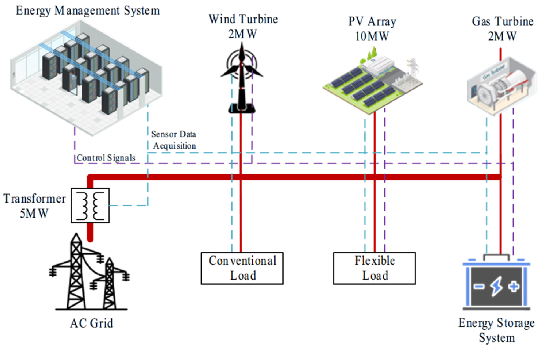
The structure of the county-level microgrid investigated in this study is illustrated in Figure 1. The microgrid integrates photovoltaic generation, wind power generation, micro gas turbines, and a battery energy storage system (BESS). The system is connected to the external utility grid and possesses bidirectional power flow capability, enabling both electricity purchasing from the grid and the feed-in of surplus renewable energy power back to the utility network.

The operational states and capacity configuration of the system are constrained by multiple factors, including the internal physical architecture of the microgrid and the operating boundary conditions of each device. Only globally feasible solutions satisfying all operational constraints possess practical engineering significance.

To achieve an optimal balance between solution accuracy and computational efficiency, this study applies mixed-integer linearization to the core physical constraints and operating mechanisms of the microgrid components. A Multi-Objective Mixed Integer Linear Programming (MILP) model is thereby established, ensuring that the proposed framework can accurately characterize the operational characteristics of the microgrid system while maintaining high computational efficiency.

2.1. Power Balance Constraint

The microgrid system must satisfy the power supply–demand balance constraint at any time instant:

$$\begin{array}{l}{P}_{pv}(t)+P_{wind}(t)+P_{gt}(t)+P_{buy}(t)+P_{dis}(t)=\\ P_{load}^{actual}(t)+P_{sell}(t)+P_{ch}(t)+P_{curt}(t)+P_{unmet}(t)\end{array}$$

(1)

where $P_{pv}(t)$ and $P_{wind}(t)$ denote the active power outputs of photovoltaic generation and wind power generation at time period $t$, respectively, obtained from day-ahead power forecasting results; $P_{gt}(t)$ represents the active power output of the micro gas turbine at time period $t$; $P_{buy}(t)$ denotes the electricity purchasing power of the microgrid from the main grid at time period $t$; $P_{dis}(t)$ represents the discharging active power of the energy storage battery at time period $t$; $P_{load}^{actual}(t)$ denotes the actual total electrical load demand of the microgrid at time period $t$ after considering load shifting; $P_{sell}(t)$ represents the electricity selling power of the microgrid to the main grid at time period $t$; $P_{ch}(t)$ denotes the charging active power of the energy storage battery at time period $t$; $P_{curt}(t)$ represents the total curtailed renewable power that cannot be accommodated by the microgrid at time period $t$; and $P_{unmet}(t)$ denotes the unmet load deficit power at time period $t$ caused by generation limits and energy storage depletion.

Considering the flexible response capability of demand-side users, load-side resources can indirectly participate in fluctuation mitigation from the demand side. After equivalent substitution, the actual baseline load participating in the integrated system operation, denoted as $P_{load}^{actual}(t)$, can be expressed as:

$$P_{load}^{actual}(t)=P_{load}(t)+P_{dr}^{up}(t)-P_{dr}^{down}(t)$$

(2)

where $P_{load}(t)$ denotes the original baseline load forecast value of the microgrid at time period $t$; $P_{dr}^{up}(t)$ represents the load power shifted into (increased during) time period $t$ by users; and $P_{dr}^{down}(t)$ denotes the load power shifted out of (reduced during) time period t by users.

2.2. Operational Constraints of the Energy Storage System

2.2.1. Boundary Constraint on Planned Capacity Limits

Under the constraints imposed by physical land occupation within the park, safety and fire protection assessments, and project investment costs, the volume and expandable margin of newly constructed energy storage stations are not unlimited:

$$E_{ess}^{min}\le x_{ess}\le E_{ess}^{max}$$

(3)

where $E_{ess}^{min}$ denotes the mandatory lower bound of the energy storage installed capacity defined by project planning requirements; $x_{ess}$ represents the decision variable of the configured energy storage capacity during the optimization process; and $E_{ess}^{max}$ denotes the physical upper expansion limit of the microgrid energy storage system constrained by external factors.

2.2.2. Dynamic Constraints of State of Charge (SOC)

The state of charge (SOC) of the energy storage system must remain continuous between two adjacent time periods. Meanwhile, the self-discharge loss and charging/discharging efficiencies of the storage system should also be taken into consideration. The SOC dynamic constraint can be expressed as:

$$E_{bat}(t)=(1-{\rho }_{sd})E_{bat}(t-1)+{\eta }_{ch}{P}_{ch}(t)-{\displaystyle \frac{P_{dis}(t)}{{\eta }_{dis}}}$$

(4)

where $E_{bat}(t)$ and $E_{bat}(t-1)$ denote the SOC of the energy storage system at time periods $t$ and $t-1$, respectively; ${\eta }_{ch}$ represents the charging efficiency of the energy storage system; $P_{ch}(t)$ and $P_{dis}(t)$ denote the charging power and discharging power of the energy storage system at time period $t$, respectively; and ${\eta }_{dis}$ denotes the discharging efficiency of the energy storage system.

2.2.3. Available SOC Constraint

To avoid rapid battery degradation caused by internal cell overcharging or overdischarging due to excessive pursuit of pure energy arbitrage, upper and lower SOC limits must be imposed on the energy storage system:

$$SO{C}_{min}{x}_{ess}\le E_{bat}(t)\le SO{C}_{max}{x}_{ess}$$

(5)

where $SO{C}_{min}$ and $SO{C}_{max}$ denote the minimum and maximum allowable SOC values, respectively.

2.2.4. Charging and Discharging Power Constraints

Since the energy storage system cannot perform charging and discharging simultaneously, mutually exclusive logical constraints for charging and discharging operations must be imposed:

$$u_{ch}(t)+u_{dis}(t)\le 1$$

(6)

$$P_{ch}(t)\le M\times u_{ch}(t)$$

(7)

$$P_{dis}(t)\le M\times u_{dis}(t)$$

(8)

where $u_{ch}(t)$ and $u_{dis}(t)$ denote the binary logical state variables for charging and discharging operations, respectively, and $M$ represents the sufficiently large constant used in the Big-M method. Meanwhile, to avoid excessive charging and discharging power rates that may lead to thermal accumulation and accelerated lifetime degradation of the energy storage system, the maximum charging/discharging power limits must be imposed. In addition, due to the influence of converter characteristics and low-level circuit topology, circuit efficiency becomes extremely low under light-load conditions. Therefore, the minimum charging/discharging power constraints of the energy storage system should also be considered:

$$k_{min}{r}_{power}{x}_{ess}-M(1-u_{ch}(t))\le P_{ch}(t)\le r_{power}{x}_{ess}$$

(9)

$$k_{min}{r}_{power}{x}_{ess}-M(1-u_{dis}(t))\le P_{dis}(t)\le r_{power}{x}_{ess}$$

(10)

where $k_{min}$ denotes the operational tolerance coefficient, and $r_{power}$ represents the maximum charging/discharging rate. In this study, the maximum charging/discharging rate is set to $0.5$.

2.2.5. Health-Oriented Charging and Discharging Management

To ensure that the energy storage system retains sufficient available capacity for normal system operation on the following day, the end-of-day SOC state is required to remain consistent with the initial SOC state:

$$E_{bat}(T)\ge SO{C}_{initial}{x}_{ess}$$

(11)

where $E_{bat}(T)$ denotes the SOC state of the energy storage system at the end of the day $t=24$; and $SO{C}_{initial}$ represents the initial SOC value at the beginning of the day. Meanwhile, to prevent accelerated battery degradation caused by frequent charging and discharging cycles within a short period, a health-oriented charging/discharging strategy is adopted, in which the energy storage system is restricted to no more than two complete charge–discharge cycles per day:

$$u_{start}^{ch}(t)\ge u_{ch}(t)-u_{ch}(t-1)$$

(12)

$$u_{start}^{dis}(t)\ge u_{dis}(t)-u_{dis}(t-1)$$

(13)

$${\displaystyle \sum _{t=1}^T{u}_{start}^{ch}}(t)\le N_{ch}^{max}$$

(14)

$${\displaystyle \sum _{t=1}^T{u}_{start}^{dis}}(t)\le N_{dis}^{max}$$

(15)

where $u_{start}^{ch}(t)$ denotes the binary start-up state variable for charging operation. A value of 1 indicates that a charging start-up action occurs during time period $t$; otherwise, the value is 0. Similarly, $u_{start}^{dis}(t)$ denotes the binary start-up state variable for discharging operation. A value of 1 indicates that a discharging start-up action occurs during time period $t$; otherwise, the value is 0. $N_{ch}^{max}$ and $N_{dis}^{max}$ represent the maximum allowable numbers of charging and discharging start-up actions scheduled within one day, respectively. For the case of two charging and two discharging cycles per day, both $N_{ch}^{max}$ and $N_{dis}^{max}$ are set to 2. Meanwhile, to avoid accelerated degradation of charging/discharging circuits caused by frequent switching between charging and discharging states within a short period, the model further imposes a minimum continuous operating duration constraint. Once the energy storage system enters either charging or discharging mode, the corresponding operating state must be maintained continuously for at least $T_{minOn}$ time periods:

$${\displaystyle \sum _{k=t}^{\min (t+T_{minOn}-1,T)}{u}_{ch}}(k)\ge \min (T_{minOn},T-t+1)\cdot u_{start}^{ch}(t)$$

(16)

$${\displaystyle \sum _{k=t}^{\min (t+T_{minOn}-1,T)}{u}_{dis}}(k)\ge \min (T_{minOn},T-t+1)\cdot u_{start}^{dis}(t)$$

(17)

where $T_{minOn}$ denotes the minimum required continuous operating duration after a single charging or discharging start-up of the energy storage system. In this study, $T_{minOn}$ is set to 2. $T$ represents the total number of scheduling periods within one day, which is set to 24 in this paper. $k$ is a sliding variable used for cumulative summation over the future time window. The $\min ()$ function is adopted to avoid boundary overflow issues at the end of the scheduling horizon.

2.3. Flexible Load Response Constraints

Demand response is an important approach for enhancing the operational flexibility of microgrids. In this model, a shiftable demand response mechanism is mainly considered, in which users are encouraged to shift part of their flexible loads, such as industrial transferable peak loads and large-scale air-conditioning cold storage equipment, to cooperate with the energy storage system in achieving peak shaving and valley filling. However, considering users’ basic electricity consumption experience and normal production requirements, the amount of load shifting is constrained by both physical limitations and user willingness. Moreover, within a complete scheduling cycle, the total cumulative electricity consumption of users should remain unchanged.

2.3.1. Upper Limit of Single-Period Load Shifting Capacity

At any time period, the load power participating in demand-side shifting regulation, including both shifted-in and shifted-out loads, shall not exceed a certain proportion of the original load demand in that period, so as to avoid excessive disturbance to users’ basic electricity consumption requirements:

$$0\le P_{dr}^{up}(t)\le {\lambda }_{dr}{P}_{load}(t)$$

(18)

$$0\le P_{dr}^{down}(t)\le {\lambda }_{dr}{P}_{load}(t)$$

(19)

where $P_{dr}^{up}(t)$ denotes the load power shifted into (increased during) time period $t$ by users in response to electricity price signals, while $P_{dr}^{down}(t)$ represents the load power shifted out of (reduced during) time period $t$ due to demand response participation. ${\lambda }_{dr}$ denotes the maximum allowable proportion of demand-responsive load relative to the total load demand at the current time period. In this study, ${\lambda }_{dr}$ is set to 15%.

2.3.2. Energy Conservation Constraint Within the Scheduling Horizon

Within the entire scheduling horizon $T$, the electrical energy reduced through load shifting by users must be compensated by an equivalent amount of shifted load in preceding or subsequent periods. Therefore, the total shifted-out load must be exactly equal to the total shifted-in load:

$${\displaystyle {\displaystyle \sum _{t=1}^T}{P}_{dr}^{up}}(t)={\displaystyle {\displaystyle \sum _{t=1}^T}{P}_{dr}^{down}}(t)$$

(20)

2.4. Grid Transaction Constraints

2.4.1. Transformer Capacity Constraint

Throughout the entire scheduling horizon T, the electrical energy reduced through load shifting by users must be compensated by an equivalent amount of shifted load in preceding or subsequent periods. Therefore, the total shifted-out load must be equal to the total shifted-in load:

$$0\le P_{buy}(t)\le P_{grid}^{max}\cdot u_{buy}(t)$$

(21)

$$0\le P_{sell}(t)\le P_{grid}^{max}\cdot u_{sell}(t)$$

(22)

$$u_{buy}(t)+u_{sell}(t)\le 1$$

(23)

where $P_{grid}^{max}$ denotes the maximum bidirectional transmission power permitted by the transformer. $u_{buy}(t)$ and $u_{sell}(t)$ are binary variables representing the electricity purchasing and selling states of the microgrid at time period $t$, respectively. When the microgrid is in either the electricity purchasing or selling state, the corresponding binary variable is equal to 1; otherwise, it is equal to 0.

2.4.2. Reverse Power Flow Constraint

Due to the high penetration level of photovoltaic generation in the county-level microgrid scenario considered in this study, restrictions on the electricity selling power are required in order to satisfy local renewable energy consumption requirements:

$$P_{sell}(t)\le P_{sell}^{max}$$

(24)

where $P_{sell}^{max}$ denotes the maximum allowable electricity export power of the microgrid.

2.4.3. Grid Interaction Ramping Constraint

If the variation in the power exchanged between the microgrid and the main grid exhibits excessive step changes between adjacent scheduling intervals, severe load fluctuations may be imposed on the utility grid. Therefore, ramping rate constraints are imposed on the grid interaction power between consecutive time periods:

$$-\Delta P_{grid}\le P_{ne{t}_{grid}}(t)-P_{ne{t}_{grid}}(t-1)\le \Delta P_{grid}$$

(25)

$$P_{ne{t}_{g}rid}(t)=P_{buy}(t)-P_{sell}(t)$$

(26)

where $\Delta P_{grid}$ denotes the maximum allowable ramping magnitude that can be tolerated by the utility grid, and $P_{ne{t}_{grid}}\left(t\right)$ represents the net active power exchanged between the microgrid and the main grid at time period $t$.

2.5. Operational Constraints of the Micro Gas Turbine

The operating power of the micro gas turbine shall not exceed its rated capacity specified on the nameplate. Meanwhile, in order to ensure stable combustion inside the combustion chamber and to maintain equipment lifetime, the output power must not be lower than a specified minimum threshold:

$$P_{gt}^{min}\cdot u_{gt}(t)\le P_{gt}(t)\le P_{gt}^{max}\cdot u_{gt}(t)$$

(27)

where $P_{gt}^{min}$ and $P_{gt}^{max}$ denote the minimum and maximum allowable operating power of the micro gas turbine, respectively. $u_{gt}(t)$ is a binary variable representing the operating state of the micro gas turbine. When the micro gas turbine is in operation, $u_{gt}(t)=1$; otherwise, $u_{gt}(t)=0$.

2.6. Natural Boundary Constraints on Renewable Energy Curtailment and Load Shedding

Under extreme operating conditions, such as excessively high renewable energy generation accompanied by very low available load demand, or sudden load surges with insufficient dispatchable energy resources, the microgrid may be forced to curtail renewable energy generation or shed part of the critical loads. Therefore, corresponding natural boundary constraints should be imposed.

2.6.1. Upper Limit Constraint on Renewable Energy Curtailment

At any time period, the amount of curtailed renewable energy in the microgrid system shall not exceed the total theoretically available power generated by wind and photovoltaic sources during the corresponding period:

$$0\le P_{curt}(t)\le P_{pv}(t)+P_{wind}(t)$$

(28)

where $P_{curt}(t)$ denotes the total curtailed wind and photovoltaic power at time period t.

2.6.2. Upper Limit Constraint on Load Shedding Power

The maximum unmet load power in the microgrid shall not exceed the total forecasted load demand at the corresponding time period:

$$0\le P_{unmet}(t)\le P_{load}(t)$$

(29)

where $P_{unmet}(t)$ denotes the unmet load power of the microgrid at time period t.

2.7. Objective Function Formulation

During the operation of clustered microgrids, inherent conflicts exist among economic performance, environmental benefits, and grid-support capability. Pursuing extreme economic efficiency may lead to increased carbon emissions or insufficient grid-support capability; excessive emphasis on low-carbon operation may increase operational costs; meanwhile, solely improving grid-support capability may sacrifice both economic and environmental performance. Therefore, this study adopts a bi-level optimization framework. In the upper-level planning layer, economic performance, low-carbon operation, and reliability are considered as optimization objectives, and the NSGA-II multi-objective optimization algorithm is employed to obtain the Pareto-optimal solution set. In the lower-level operational scheduling layer, the energy storage configuration determined by the upper-level optimization is taken as the input parameter, and an MILP model is established accordingly.

By introducing fixed subjective preference weighting coefficients, the three objectives of economy, low carbon, and reliability in day-ahead scheduling are transformed into a single-objective optimization problem aimed at minimizing the comprehensive operational cost. In this manner, the lower-level scheduling model provides realistic operational dispatch schemes and economic evaluation indicators for the fitness assessment of the upper-level optimization process.

2.7.1. Upper-Level Multi-Objective Capacity Configuration Model

In the upper-level model, the rated configured capacity of the energy storage units within the clustered microgrid system, denoted by $x_{ess}$, is selected as the core decision variable. The model adopts the minimum annualized comprehensive investment and operational cost, the minimum annual total carbon dioxide emissions, and the maximum peak-shaving contribution rate as quantitative indicators representing economic performance, low-carbon operation, and reliability, respectively. Accordingly, the multi-objective optimization problem can be formulated as follows:

$$\min F(x_{ess})={[F_{econ}(x_{ess}),F_{env}(x_{ess}),-F_{peak}(x_{ess})]}^T$$

(30)

where $F(x_{ess})$ denotes the multi-objective fitness evaluation vector function; $F_{econ}(x_{ess})$ represents the comprehensive cost of the microgrid system, consisting of annualized investment depreciation and actual economic operating costs; $F_{env}(x_{ess})$ denotes the annual total carbon dioxide emissions of the microgrid system; and $F_{peak}(x_{ess})$ represents the peak-shaving contribution rate of the energy storage system during grid peak-load periods.

The peak-shaving contribution rate is an important indicator used to evaluate regional grid interaction flexibility and power supply reliability. It is defined as the ratio between the total energy storage discharging power during peak-load periods and the total baseline load demand within the same periods:

$$F_{peak}(x_{ess})={\displaystyle \frac{{\displaystyle \sum _{t\in T_{peak}}{P}_{dis}}(t)}{{\displaystyle \sum _{t\in T_{peak}}{P}_{load}}(t)}}\times 100\%$$

(31)

where $T_{peak}$ denotes the set of grid peak-load periods determined according to the time-of-use electricity pricing scheme.

2.7.2. Lower-Level Operational Scheduling Model of the Microgrid System

To comprehensively evaluate multiple scheduling attributes and obtain a unique optimal day-ahead operational scheduling scheme under a given storage capacity configuration, the lower-level model introduces a set of predefined weighting coefficients to combine multiple performance indicators into a weighted comprehensive objective function for minimization:

$$\min F_{total}^{run}=w_{econ}{f}_{econ}^{run}+w_{env}{f}_{env}^{run}+w_{rel}{f}_{rel}^{run}$$

(32)

where $F_{total}^{run}$ denotes the weighted comprehensive virtual operating cost used to guide the day-ahead output scheduling of the system equipment. $w_{econ}$, $w_{env}$ and $w_{rel}$ represent the fixed preference weighting coefficients corresponding to economy, low-carbon performance, and reliability, respectively, satisfying the condition that their sum equals 1. In the case study of this paper, an economy-oriented strategy is adopted, and the weighting coefficients are set to 0.8, 0.1, and 0.1, respectively. It should be noted that these weights serve only to compute a well-defined comprehensive operating cost for the lower-level MILP dispatch. The multi-criteria decision-making in this study is performed at the upper level, where NSGA-II treats economy, carbon emissions, and reliability as independent objectives to generate a Pareto frontier, from which planning decisions are made without reliance on pre-specified weights. $f_{econ}^{run}$ denotes the lower-level economic operating cost objective function; $f_{env}^{run}$ represents the lower-level low-carbon penalty objective function, namely, the equivalent carbon emission penalty cost; and $f_{rel}^{run}$ denotes the lower-level reliability penalty objective function, namely, the equivalent penalty cost associated with unmet load demand. Specifically, the detailed formulations of the three lower-level objective costs are given as follows:

(1)

Economic Objective

This objective aims to minimize the daily operational expenditure and the depreciation cost of the initial investment of the microgrid system. The cost components mainly include the annualized investment cost of the energy storage equipment, electricity purchasing and selling transaction costs, fuel consumption and start-up/shut-down operation and maintenance costs of the micro gas turbine, penalty costs associated with renewable energy curtailment, as well as compensation costs incurred by the implementation of demand response. The lower-level economic objective function $f_{econ}^{run}$ can be expressed as follows:

$$f_{econ}^{run}=C_{inv}^{ESS}+C_{grid}+C_{GT}+C_{curt}+C_{DR}$$

(33)

Specifically, each cost component can be expressed as follows:

$$C_{inv}^{ESS}=c_{inv}^{ess}\cdot x_{ess}$$

(34)

$$C_{grid}=D\cdot {\displaystyle \sum _{t=1}^T\left(p_{buy}(t)P_{buy}(t)-p_{sell}(t)P_{sell}(t)\right)}$$

(35)

$$C_{GT}=D\cdot {\displaystyle \sum _{t=1}^T\left(c_{fuel}{P}_{gt}(t)+c_{om}^{gt}{u}_{gt}(t)\right)}$$

(36)

$$C_{curt}=D\cdot c_{curt}{\displaystyle \sum _{t=1}^T{P}_{curt}}(t)$$

(37)

$$C_{DR}=D\cdot c_{dr}{\displaystyle \sum _{t=1}^T(P_{dr}^{up}(}t)+P_{dr}^{down}(t))$$

(38)

where $C_{inv}^{ESS}$ denotes the annualized cost of the energy storage system; $c_{inv}^{ess}$ represents the annualized unit capacity investment cost of energy storage; $C_{grid}$ denotes the net interaction cost between the microgrid and the utility grid; $D$ represents the number of operating days per year, which is set to 365 in this study; $p_{buy}(t)$ and $p_{sell}(t)$ denote the time-of-use electricity prices for purchasing electricity from and selling electricity to the utility grid at time period $t$, respectively; $C_{GT}$ denotes the annualized operating cost of the micro gas turbine; $c_{fuel}$ represents the unit fuel cost converted from natural gas consumption based on calorific value equivalence; $c_{om}^{gt}$ denotes the operation and maintenance cost of the micro gas turbine per scheduling period under operating conditions; $C_{curt}$ denotes the annualized penalty cost associated with wind and photovoltaic curtailment; $c_{curt}$ represents the penalty price per unit curtailed renewable energy; $C_{DR}$ denotes the annual compensation cost paid by the microgrid to users for participating in demand response load shifting; and $c_{dr}$ represents the compensation coefficient for demand response regulation per unit power.

(2)

Low-Carbon Objective

Considering the interaction between energy supply and demand within the microgrid, this objective not only includes the direct carbon emissions generated by the internal combustion of fossil fuels in the micro gas turbine but also takes into account the indirect equivalent carbon emission intensity associated with electricity purchased from the utility grid:

$$f_{env}^{run}=D\cdot p_{carbon}{\displaystyle \sum _{t=1}^T\left(e_{gt}{P}_{gt}(t)+e_{grid}(P_{buy}(t)-P_{sell}(t))\right)}$$

(39)

where $p_{carbon}$ denotes the carbon price per unit of carbon dioxide in the carbon trading market; $e_{gt}$ represents the carbon dioxide emission factor per unit output power of the micro gas turbine; and $e_{grid}$ denotes the carbon emission intensity of the utility grid.

(3)

Reliability Objective

This objective imposes a high virtual penalty cost on interrupted or unmet load demand, thereby encouraging the scheduling model to utilize all available flexible resources to avoid load shedding. Meanwhile, it also prevents the model from excessively relying on renewable energy generation and electricity trading with the utility grid for profit-seeking purposes that may result in power shortages:

$$f_{rel}^{run}=D\cdot p_{penalty}{\displaystyle \sum _{t=1}^T{P}_{unmet}}(t)$$

(40)

where $p_{penalty}$ denotes the penalty cost associated with unmet load demand.

3. Solution Methodology of the Bi-Level Optimization Model

3.1. Model Solution Procedure

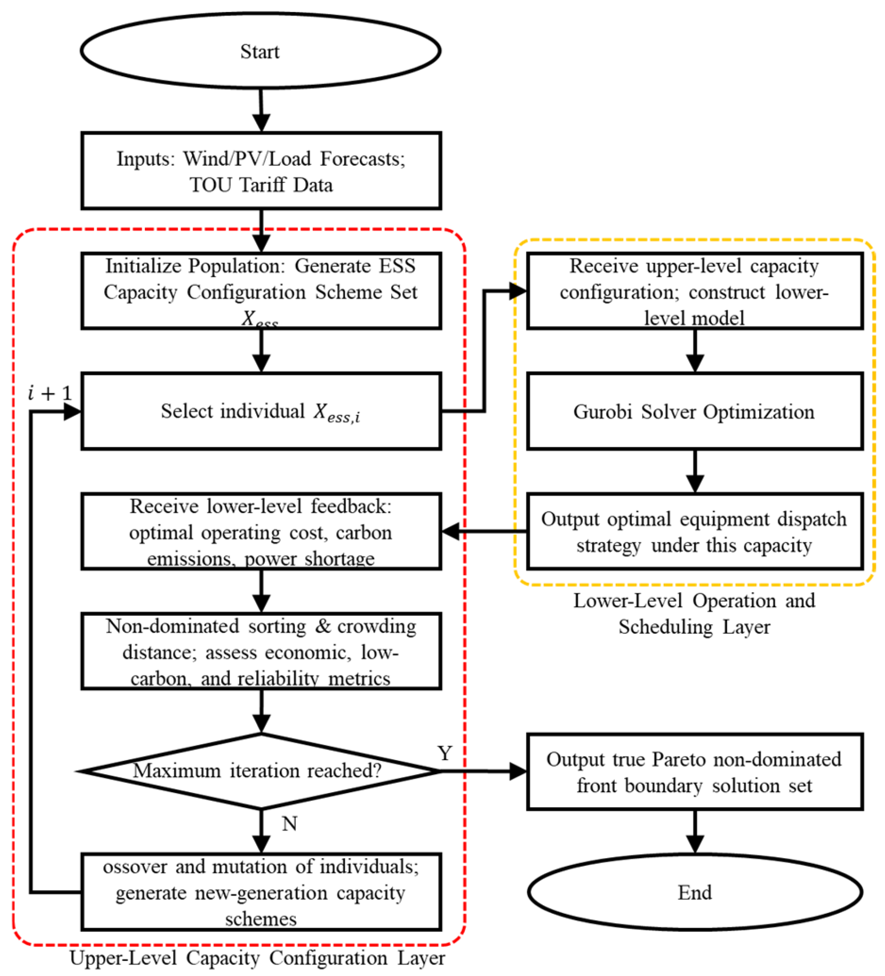
For the multi-objective bi-level optimization model developed in this study, the complete internal computational loop and feedback-based game-theoretic solution procedure are illustrated in Figure 2. The flowchart intuitively demonstrates the iterative interaction mechanism between the upper-level capacity configuration model and the lower-level operational scheduling model. The lower-level MILP dispatch model is solved using the Gurobi Optimizer via the YALMIP interface in MATLAB 2024.

3.2. Core Mechanisms of the NSGA-II Algorithm

Fast non-dominated sorting is used to classify the entire population into different Pareto ranks according to the dominance relationships among individuals. For each individual in the population, the number of times it is dominated and the set of individuals it dominates are calculated, based on which the Pareto rank is determined. Individuals with higher ranks are closer to the true Pareto frontier, thereby enabling rapid screening of high-quality solutions.

Crowding distance is adopted to measure the sparsity degree of individuals in the objective space. By calculating the sum of the distances between each individual and its neighboring individuals in each objective dimension, the crowding distance value can be obtained. A larger crowding distance indicates that the corresponding region contains a sparser distribution of individuals. Preserving such individuals helps maintain the diversity of the solution set and prevents the algorithm from converging to local optimal solutions.

During the iterative optimization process, an elite preservation strategy is introduced by merging the parent population and offspring population. Fast non-dominated sorting and crowding distance calculation are then performed on the merged population. Individuals are selected according to Pareto rank and crowding distance to form the next-generation population. This strategy ensures that high-quality genes are not lost during the iterative process, thereby effectively improving the convergence speed and optimization performance of the algorithm.

4. Case Study Analysis

4.1. Parameter Setting of the Microgrid Model

The capacity parameters of distributed generation units and key equipment are listed in

Table 1. Rated capacity of each distributed power source and equipment.

Parameter	Value
Rated installed capacity of photovoltaic generation	10 MW
Rated installed capacity of wind power generation	2 MW
Rated capacity of micro gas turbine	2 MW
Minimum technical output of micro gas turbine	0.3 MW
Capacity of utility grid interconnection transformer	5 MW
Battery energy storage system	Limited to 0.1~15 MWh

, while the cost parameters are provided in

Table 2. Model parameter table.

Parameter	Symbol	Value	Unit
Lower limit of energy storage installed capacity	$E_{ess}^{min}$	0.1	MWh
Upper limit of energy storage installed capacity	$E_{ess}^{max}$	15	MWh
Charging efficiency of energy storage system	${\eta }_{ch}$	0.93	-
Discharging efficiency of energy storage system	${\eta }_{dis}$	0.93	-
Minimum SOC	$SO{C}_{min}$	0.15	-
Maximum SOC	$SO{C}_{max}$	0.85	-
Operating tolerance coefficient	$k_{min}$	0.05	-
Initial SOC	$SO{C}_{initial}$	0.15	-
Maximum electricity selling power of microgrid	$P_{sell}^{max}$	2	MW
Maximum ramping limit of utility grid	$\Delta P_{grid}$	3	MW
Minimum operating power of micro gas turbine	$P_{gt}^{min}$	0.3	MW
Maximum operating power of micro gas turbine	$P_{gt}^{max}$	2	MW
Annualized unit investment cost of energy storage capacity	$c_{inv}^{ess}$	1.89	104 CNY/MWh/year
Unit fuel cost per electricity consumption	$c_{fuel}$	1.085	CNY/kWh
Operation and maintenance cost of micro gas turbine	$c_{om}^{gt}$	5	CNY/h
Annualized penalty cost of renewable energy curtailment	$C_{curt}$	50	CNY/kWh
Compensation cost for unit demand response scheduling	$c_{dr}$	0.2	CNY/kWh
Unit carbon dioxide pricing in carbon trading market	$p_{carbon}$	0.1	CNY/kgCO2
Carbon dioxide emissions per unit power output of micro gas turbine	$e_{gt}$	0.5	kg/kWh
Carbon emission intensity of utility grid	$e_{grid}$	0.85	kg/kWh
Penalty cost for unmet load demand	$p_{penalty}$	100	CNY/kWh
Big-M constant	$M$	107	-

. The parameter settings comprehensively consider the actual operational characteristics of county-level power grids and typical engineering configuration levels, covering renewable energy sources, grid interaction capability, and energy storage capacity ranges, thereby providing a unified basis for subsequent multi-scenario comparative analysis.

4.2. Operational Characteristics Analysis of the Baseline Scenario Without Energy Storage

In the baseline scenario without an energy storage system, the system regulation capability mainly relies on the micro gas turbine and power interaction with the utility grid. Due to the absence of an energy buffering mechanism, the peak photovoltaic output and peak load demand exhibit significant temporal mismatch, resulting in insufficient source–load matching capability.

Source–Load Power Imbalance and Renewable Energy Curtailment Phenomenon

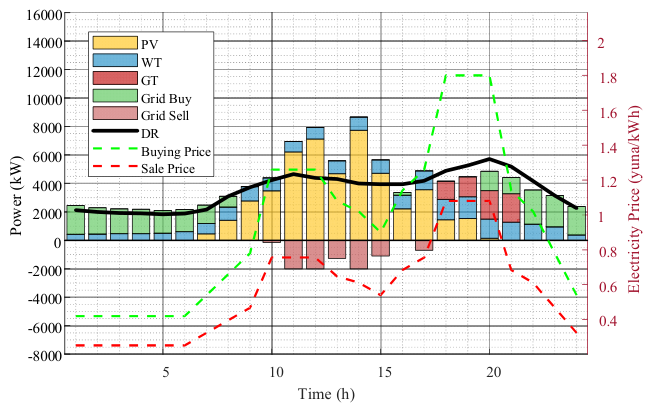
As shown in Figure 3, during the period from 10:00 to 14:00, the photovoltaic output is significantly higher than the load demand level. Restricted by the reverse power transmission capacity limit of the utility grid, part of the generated electricity cannot be accommodated. During the evening peak-load period from 18:00 to 21:00, the photovoltaic output approaches zero, while both the micro gas turbine and grid purchasing power operate close to their rated capacities. Under this condition, the system possesses a limited regulation margin, and the security of the power supply heavily depends on external grid support.

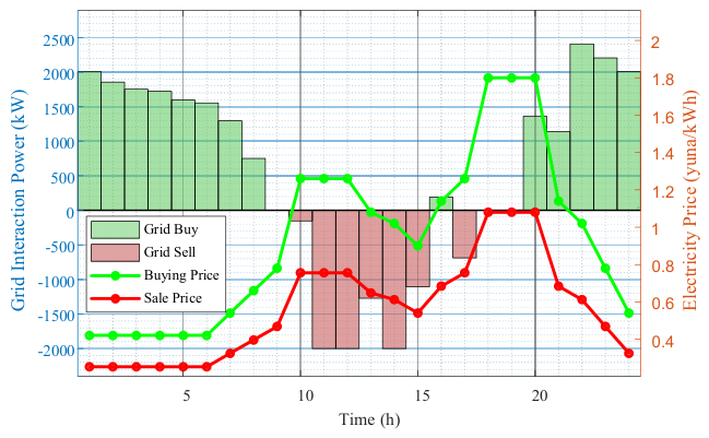
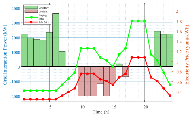
As shown in Figure 4, the electricity purchasing behavior of the system exhibits a significant passive coupling relationship with the time-of-use electricity pricing scheme. During the evening peak-price period, the purchased electricity reaches its maximum value, causing the levelized cost of electricity (LCOE) on the supply side to increase to 0.2339 CNY/kWh. During off-peak periods, the load demand is insufficient to absorb low-price electricity, and the system lacks peak–valley arbitrage capability, thereby limiting the overall economic operating efficiency.

4.3. Detailed Operational Analysis of Source–Grid–Load–Storage Coordinated Optimization

After the integration of the energy storage system, the microgrid forms a coordinated regulation structure involving the source, grid, load, and storage. Through time-domain charging and discharging scheduling, the energy storage system reconstructs the power flow distribution, enabling the system to achieve a dynamic balance between renewable energy accommodation and economic dispatch.

4.3.1. Power Flow Reconstruction and Renewable Energy Accommodation Enhancement Mechanism

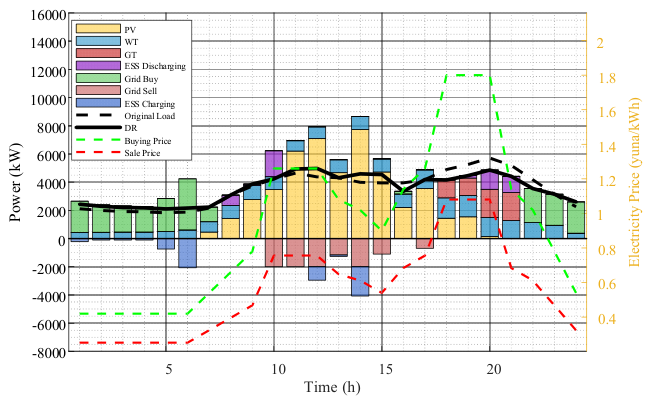
As shown in Figure 5, the energy storage system is charged during periods of high photovoltaic output and low electricity prices, while discharging occurs during the evening peak-load period to compensate for load demand. This mechanism effectively eliminates renewable energy curtailment and increases the local renewable energy accommodation rate from 95.68% to 100%, thereby achieving full absorption of distributed photovoltaic generation.

4.3.2. Verification of Energy Storage Operation Strategy and Peak-Shaving Capability

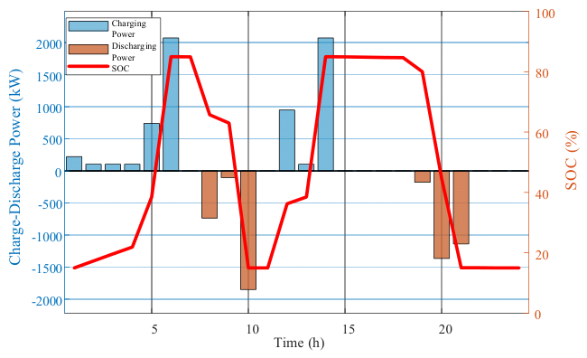
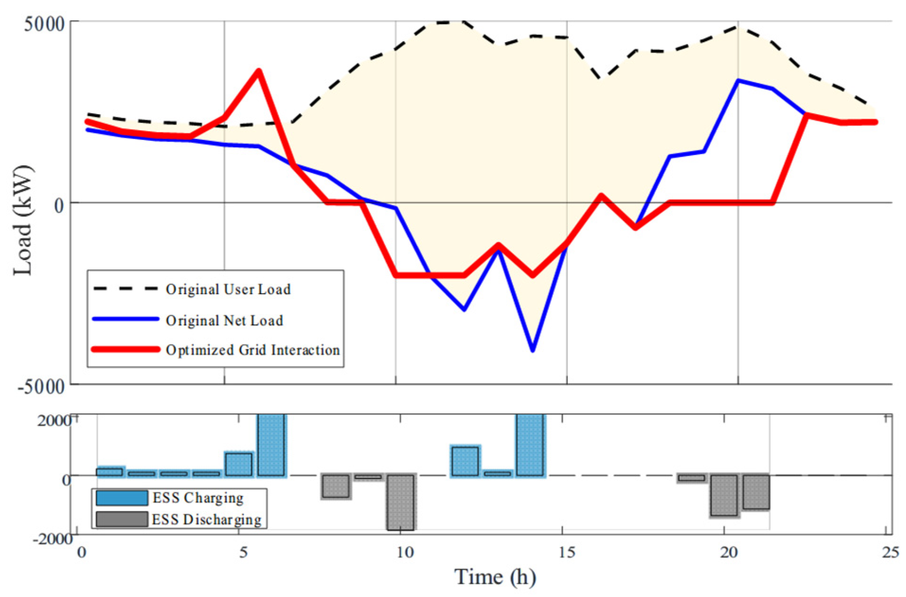
The SOC trajectory shown in Figure 6 indicates that the energy storage system operates cyclically within the range of 15–85%, realizing the “charge at low-price periods and discharge at high-load periods” strategy as well as the two-charge and two-discharge operational strategy specified in the model. Figure 7 shows that the electricity purchasing power from the utility grid decreases significantly during the evening peak-load period. The maximum peak-shaving power provided by the energy storage system accounts for 32.34% of the peak load demand, and the peak-shaving capability is improved by more than 25%. Consequently, the operational stability of the system is significantly enhanced.

4.3.3. Price Response and Economic Arbitrage

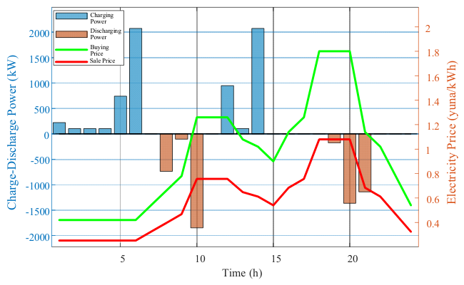
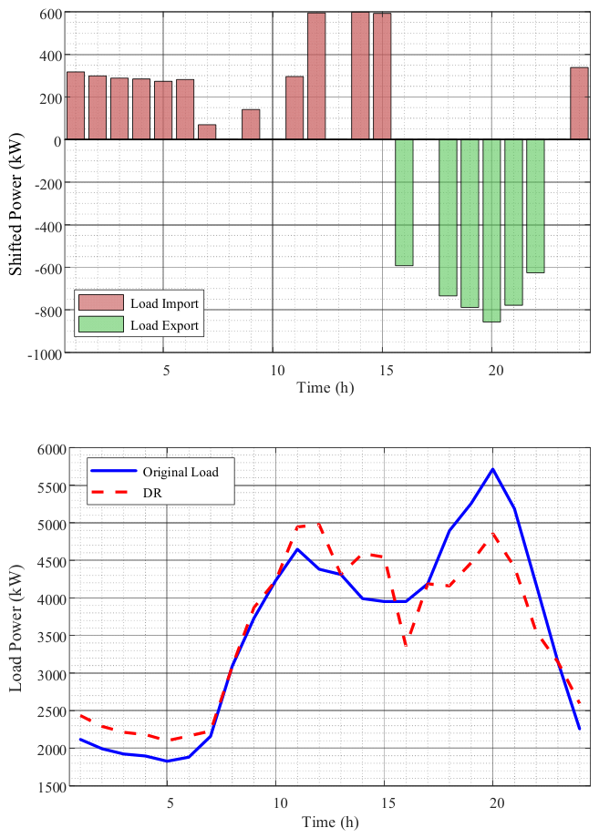
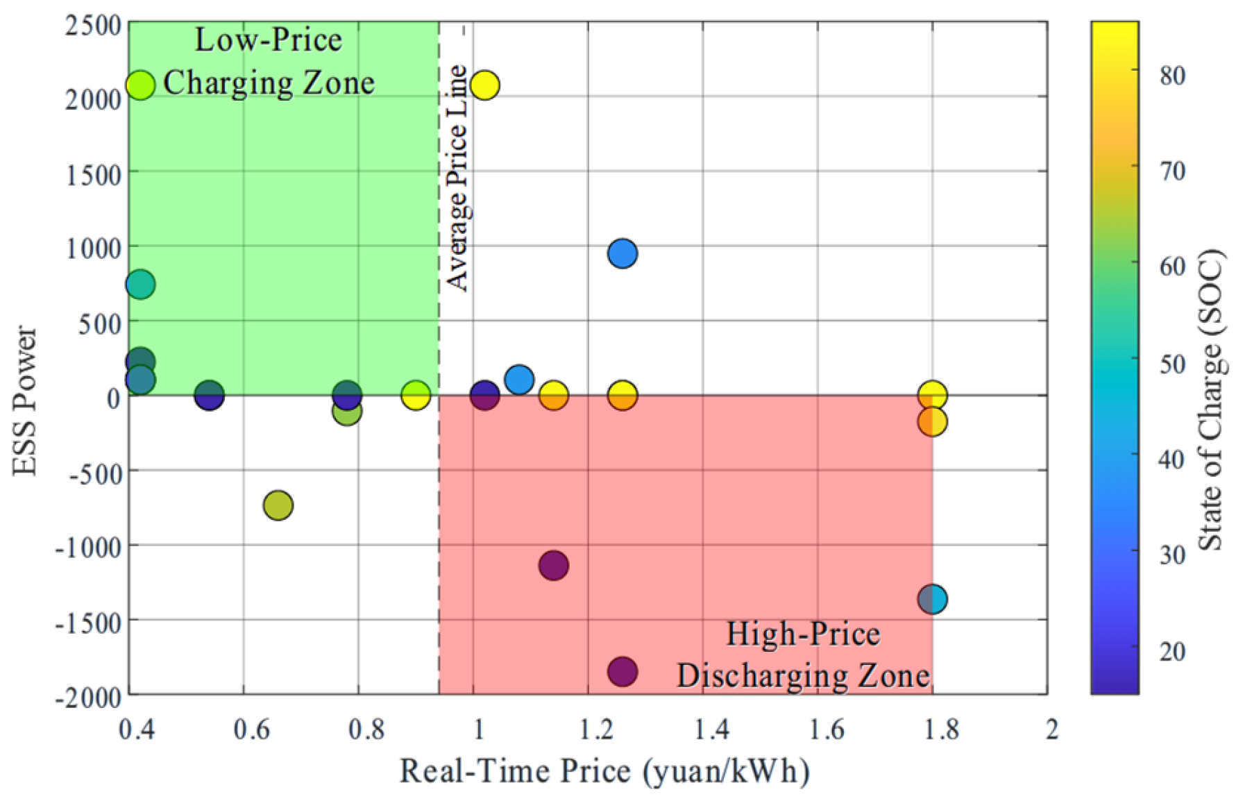
Figure 8 illustrates the coupling relationship between the charging/discharging power of the energy storage system and the time-of-use electricity price. Charging behavior is mainly concentrated in low-price periods, while discharging behavior is concentrated in high-price periods, exhibiting a clear price-driven characteristic. The scatter distribution further verifies that the optimization algorithm can accurately identify electricity price signals and achieve the objective of economic dispatch.

4.3.4. Scheduling Performance of Flexible Loads (Demand Response)

Figure 9 shows that the shiftable loads are mainly transferred from high-price periods to periods with high photovoltaic output and low electricity prices. After optimization, the peak–valley difference of the load curve is significantly reduced, and the smoothness of the load profile is improved. The demand response mechanism further alleviates the peak-shaving pressure of the system and enhances the source–load matching capability.

4.3.5. Governance Effect Under Source–Grid–Load–Storage Coordination

With the continuous increase in the penetration level of distributed photovoltaic generation in county-level regions, clustered microgrids exert increasingly significant impacts on the operational characteristics of the upstream utility grid, exhibiting a pronounced “duck curve” phenomenon. During the daytime photovoltaic peak-output period (10:00–14:00), the net load, defined as the total load minus the photovoltaic output, decreases to an extremely low level, forming the “duck belly.” After sunset, during the period of rapid photovoltaic output decline (17:00–19:00), the net load rises sharply, forming the steep “duck neck.” This imposes substantial challenges on the ramping capability of the upstream utility grid and can easily lead to problems such as voltage fluctuations and frequency instability.

As shown in Figure 10, the net load profile in the scenario without energy storage exhibits a typical “duck curve” characteristic. The energy storage system absorbs surplus power during periods of high photovoltaic generation and releases electricity after sunset, thereby significantly reducing both the depth of the “duck belly” and the ramping rate of the “duck neck.” Consequently, the impact of the microgrid system on the upstream utility grid is substantially mitigated.

4.3.6. Price Response Distribution of Energy Storage Scheduling

To verify whether the optimization algorithm can accurately capture market price signals and achieve economically optimal scheduling of the energy storage system, this section analyzes the coupling relationship between charging/discharging actions and time-of-use electricity prices through scatter distribution plots, as illustrated in Figure 11.

In Figure 11, the green scatter region represents the relationship between the charging power of the energy storage system and the time-of-use electricity price, while the red scatter region represents the relationship between the discharging power and the electricity price. From the green scatter region, it can be observed that the charging behaviors are highly concentrated within low-price periods, indicating that the optimization algorithm can accurately identify electricity price valleys for energy charging, thereby minimizing charging costs to the greatest extent. Outside the low-price intervals, almost no charging scatter points are observed, which further demonstrates the strong selectivity and economic rationality of the algorithm in determining charging timing.

From the red scatter region, it can be observed that the discharging behaviors are mainly concentrated within peak electricity price periods, during which discharging can achieve the highest economic return. In medium-price periods, the number of discharging scatter points is relatively small, and limited discharging actions occur only when the load demand is relatively high and the photovoltaic output is insufficient. In low-price periods, almost no discharging scatter points appear, thereby avoiding economic losses caused by discharging during low-price intervals.

These distribution characteristics fully demonstrate that the optimization model successfully establishes a strong coupling mechanism between electricity prices and operational actions. The energy storage system can dynamically adjust its charging and discharging strategies according to variations in time-of-use electricity prices, thereby maximizing economic benefits. The energy storage system is no longer merely a carrier for physical energy transfer but is also an amplifier of economic value. Through accurate price-responsive scheduling, it effectively supports the reduction of peak–valley electricity price differences and provides strong support for the economically optimal operation of the system.

4.4. Island Mode Resilience Verification

4.4.1. Motivation and Setup

The grid-connected optimization presented in Section 4.3 identifies 4.15 MWh as the economically optimal ESS capacity under normal operating conditions. To assess system resilience under loss of grid connection, the island mode performance is evaluated using the identical MILP dispatch framework with two modifications. First, the grid interconnection limit is set to zero ($gri{d}_{max}=0$). Second, the unmet load term $P_{unmet}$ is relocated from the right-hand side to the left-hand side of the power balance equation, enabling load shedding to function as a virtual supply source:

$$P_{pv}+P_{wind}+P_{gt}+P_{dis}+P_{unmet}={\tilde{P}}_{load}+P_{ch}+P_{curt}$$

(41)

The ESS capacity is fixed at 4.15 MWh. To reflect a realistic preparedness posture prior to islanding, the initial SOC is set to 0.15. All other parameters, including the DR mechanism (15% shiftable load ratio), remain unchanged from the grid-connected configuration.

4.4.2. Dispatch Performance

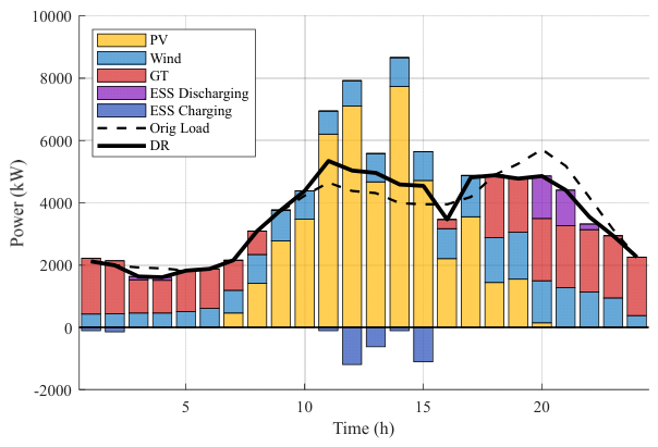
The minimum feasible initial SOC for island operation is 15% ($SO{C}_{min}$), representing the worst-case preparedness scenario in which the ESS enters islanding with no energy reserve above its operational floor. Figure 12 presents the 24 h island power flow at $SO{C}_{initial}=0.15$.

In the absence of an ESS, the island baseline yields LPSP = 3.43%, with the shortfall concentrated in the evening hours. With the 4.15 MWh ESS, LPSP decreases to 0.27%—a 92.1% reduction in unmet load. The dispatch sequence exhibits three temporal phases. During the nighttime and morning hours (hours 1–10), wind generation and GT jointly supply the load while the ESS remains idle at $SO{C}_{min}$, as no renewable surplus is available for charging. During the midday PV surplus period (hours 11–15), solar output peaks at 7111 kW at hour 12, far exceeding the instantaneous load. The ESS charges at its 0.5 C rated power of 2075 kW, rising from 15% to 85% within approximately three hours. The residual PV surplus—reaching 3970 kWh at hour 14—is curtailed, indicating that the 4.15 MWh capacity cannot absorb the full midday renewable generation. During the evening peak (hours 16–24), the ESS discharges to supplement GT and wind. At hour 20, the combined supply of PV (145 kW), wind (1349 kW), GT (2000 kW), and ESS discharge reaches its maximum, leaving a small residual deficit that produces the 0.27% LPSP.

The DR mechanism shifts approximately 1065 kWh (1.3% of daily load) from evening deficit hours to the midday period, modestly reducing the peak demand. The original and DR-adjusted load profiles are both shown in Figure 12.

4.4.3. Sensitivity of LPSP

The preceding analysis examines the worst-case $SO{C}_{initial}=0.15$. To evaluate how the preparedness level affects island resilience, $SO{C}_{initial}$ is swept from 0.15 to 0.85 in 0.05 increments.

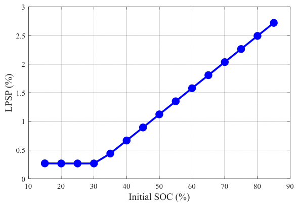
Figure 13 reveals a monotonic, near-linear relationship: LPSP rises from 0.27% at $SO{C}_{initial}=0.15$ to 2.72% at $SO{C}_{initial}=0.85$. The curve remains flat at 0.27% over the range $SO{C}_{initial}\in [0.15,0.30]$, indicating that a modest initial SOC buffer does not constrain the dispatch; the ESS can freely discharge to cover the load and still terminate above the daily cycle floor. Above $SO{C}_{initial}=0.30$, LPSP begins to rise, where the constraint binds more tightly against the available ESS discharge capacity during the evening peak.

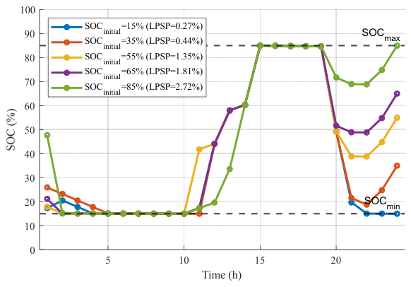
This behavior arises from the daily cycle constraint (11), which requires the ESS to end the day no lower than its initial SOC. To satisfy this condition at elevated $SO{C}_{initial}$, the optimizer restricts ESS discharge during the evening peak—preserving stored energy for end-of-day compliance—and accepts higher unmet load. At $SO{C}_{initial}=0.15$, the constraint is minimally binding and the ESS discharges freely. At $SO{C}_{initial}=0.85$, the model tolerates 2.72% LPSP to avoid depleting the ESS below the 85% threshold. The trajectories in Figure 14 confirm that all paths terminate at their respective initial SOC levels, with progressively compressed evening discharge windows at higher $SO{C}_{initial}$ values.

The daily cycle constraint was designed for grid-connected repetitive operation, where overnight grid charging restores $SO{C}_{initial}$ at minimal cost. Under emergency islanding, the priority shifts from energy neutrality to load survival. The 4.15 MWh ESS, determined on purely economic grounds in the grid-connected analysis, provides meaningful island resilience; eliminating the residual LPSP would require either a higher ESS power rating or additional GT capacity to close the evening peak power deficit.

4.5. Multi-Dimensional Comparison of Comprehensive Benefits

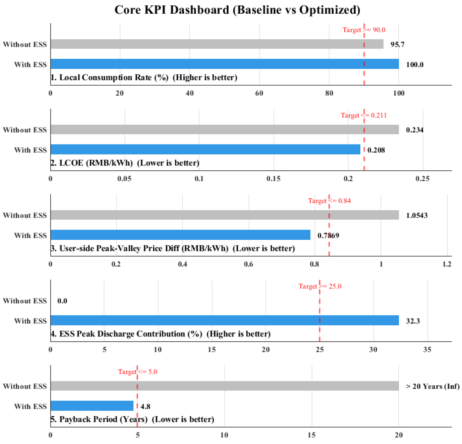
Figure 15 compares the comprehensive performance of the system before and after energy storage configuration. After integrating the energy storage system, the local renewable energy accommodation rate increases to 100%, the levelized cost of electricity (LCOE) decreases to 0.2080 CNY/kWh, the peak–valley electricity price difference on the user side is reduced by 25.37%, the peak-period discharging contribution rate reaches 32.34%, and the investment payback period is approximately 4.8 years. The results demonstrate that the integration of energy storage provides significant improvements in terms of economic performance, low-carbon operation, and system reliability.

4.6. Sensitivity Analysis and Multi-Objective Pareto Decision-Making

4.6.1. Sensitivity Analysis of Energy Storage Capacity

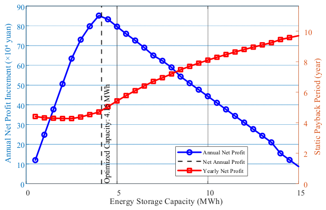
Figure 16 shows that the annual net profit exhibits a trend of increasing first and then decreasing with the growth of the energy storage capacity. When the storage capacity reaches 4.15 MWh, the economic benefit achieves its maximum value. Beyond this point, the marginal benefit gradually decreases, and the investment payback period becomes longer. The results verify that this capacity corresponds to the economically optimal configuration under the current scenario.

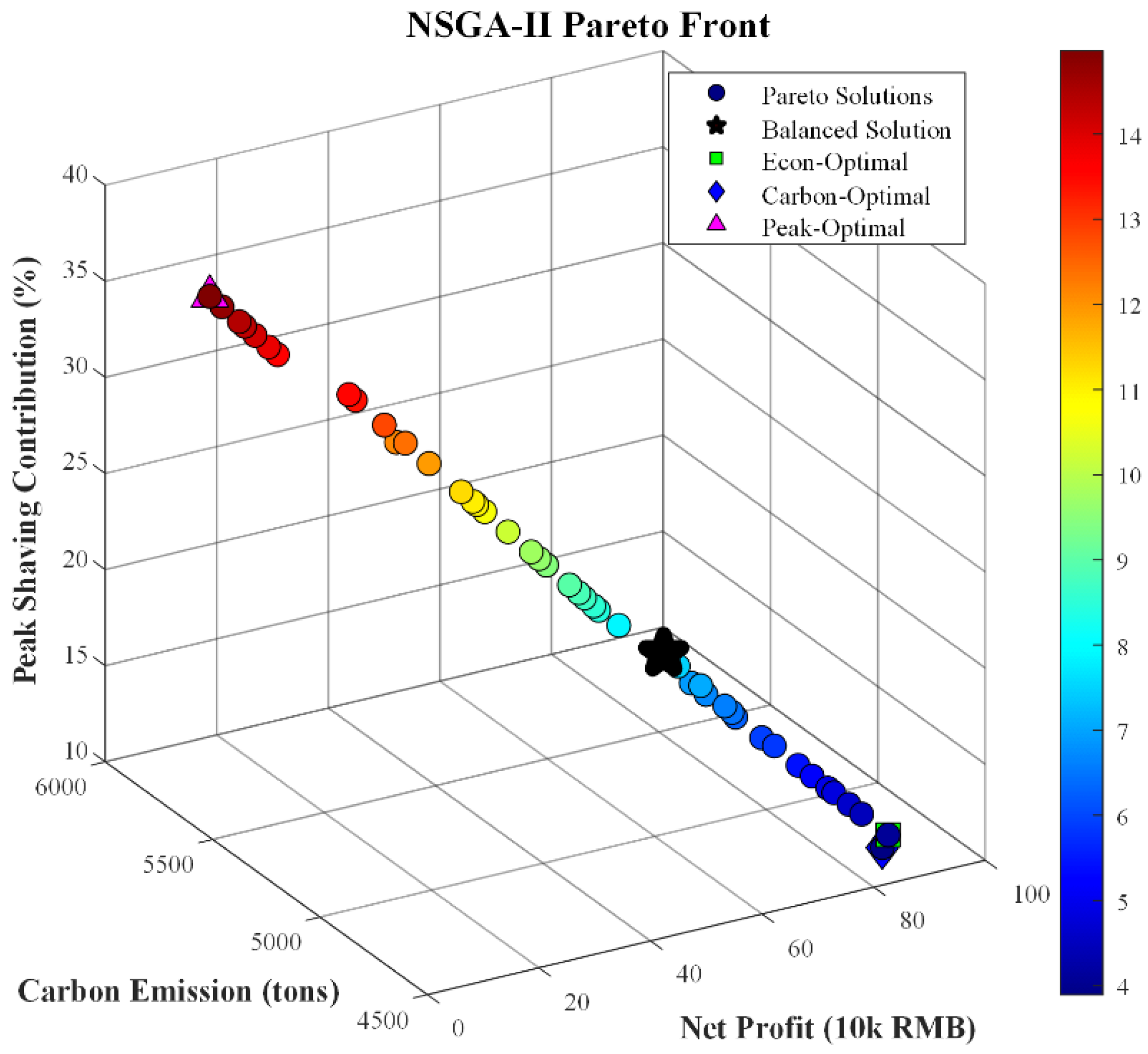
4.6.2. NSGA-II Multi-Objective Pareto Frontier Analysis

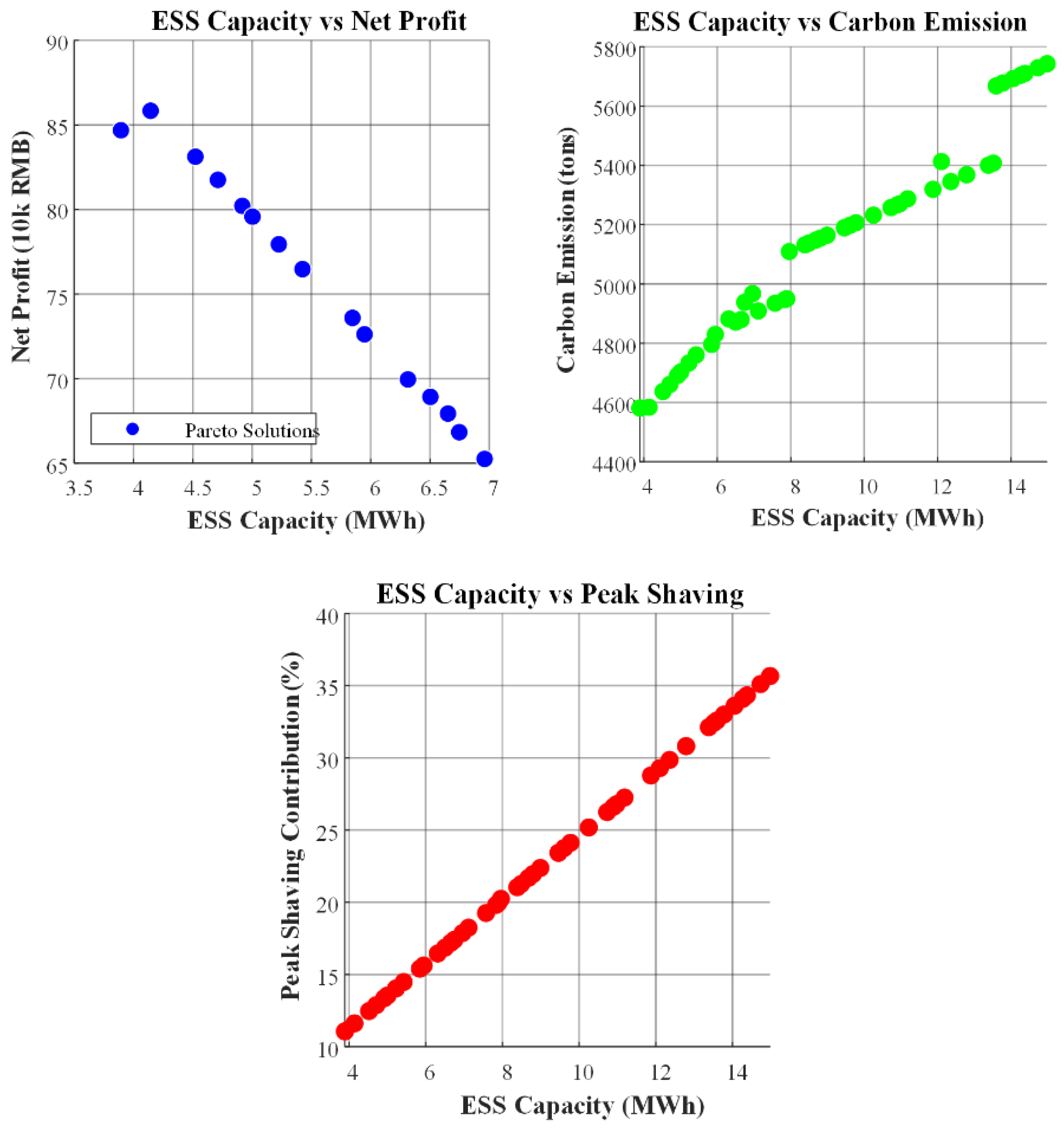
Figure 17 presents the non-dominated solution set among the economic, low-carbon, and reliability objectives. Figure 18 shows that increasing the energy storage capacity can enhance the peak-shaving capability; however, the economic benefit exhibits an extreme-value characteristic. Decision-makers can select balanced solutions along the Pareto frontier according to different operational priorities, thereby achieving coordination among multiple objectives.

5. Conclusions

This paper proposes a bi-level coordinated optimization framework integrating ESS capacity planning and operational dispatch for county-level microgrids under high distributed PV penetration. The principal quantitative findings from the case study are as follows:

(1)

The coordinated source–grid–load–storage configuration eliminates renewable curtailment (from 4.32% to 0%), reduces the levelized cost of electricity from 0.2339 to 0.2080 CNY/kWh (an 11.1% reduction), and delivers a peak-shaving contribution rate of 32.34%. The peak–valley electricity price difference on the user side is narrowed by 25.37%, and the ESS investment payback period is approximately 4.8 years.

(2)

ESS capacity expansion exhibits clear diminishing marginal returns. The annual net profit peaks at 4.15 MWh and declines thereafter, confirming the existence of an absolutely convergent economically optimal configuration capacity under the current cost structure and electricity pricing mechanism.

(3)

The three-dimensional Pareto frontier (economy–carbon–reliability) explicitly characterizes the trade-offs among competing objectives. The NSGA-II-generated non-dominated solution set converges within 20 generations (50 individuals per generation), providing decision-makers with a quantitative basis for selecting configurations according to operational priorities, without reliance on pre-specified weights.

(4)

Under island-mode operation with the economically optimal 4.15 MWh ESS, the loss of power supply probability is reduced from 3.43% (no-ESS island baseline) to 0.27%—a 92.1% reduction in unmet load. The sensitivity of the LPSP to the initial SOC reveals that the daily cycle constraint, designed for grid-connected operation, introduces a trade-off between preparedness level and resilience performance in emergency scenarios.

The current framework assumes deterministic forecasts and does not incorporate stochastic or robust optimization, detailed AC/DC network constraints, cycle-life battery degradation models, or cascading failure analysis. Addressing these aspects represents important directions for future work.

References

1. Xia, Y.; Sun, G.; Wang, Y.; Yang, Q.; Wang, Q.; Ba, S. A novel carbon emission estimation method based on electricity-carbon nexus and non-intrusive load monitoring. Appl. Energy 2024, 360, 122773. [Google Scholar] [CrossRef]
2. Li, H.; He, Y.; Fu, W.; Li, X. Bi-level planning of electric vehicle charging station in coupled distribution-transportation networks. Electr. Power Syst. Res. 2024, 232, 110442. [Google Scholar] [CrossRef]
3. Roy, N.K.; Pota, H.R. Current status and issues of concern for the integration of distributed generation into electricity networks. IEEE Syst. J. 2014, 9, 933–944. [Google Scholar] [CrossRef]
4. Mahmud, N.; Zahedi, A. Review of control strategies for voltage regulation of the smart distribution network with high penetration of renewable distributed generation. Renew. Sustain. Energy Rev. 2016, 64, 582–595. [Google Scholar] [CrossRef]
5. Jain, S.; Kalambe, S.; Agnihotri, G.; Mishra, A. Distributed generation deployment: State-of-the-art of distribution system planning in sustainable era. Renew. Sustain. Energy Rev. 2017, 77, 363–385. [Google Scholar] [CrossRef]
6. Mehigan, L.; Deane, J.P.; Gallachóir, B.Ó.; Bertsch, V. A review of the role of distributed generation (DG) in future electricity systems. Energy 2018, 163, 822–836. [Google Scholar] [CrossRef]
7. Denholm, P.; Margolis, R.M. Evaluating the limits of solar photovoltaics (PV) in electric power systems utilizing energy storage and other enabling technologies. Energy Policy 2007, 35, 4424–4433. [Google Scholar] [CrossRef]
8. Wenwen, S.; Guoqing, H.; Chun, L.; Shuanglei, F. A review of solutions for voltage beyond limits in distribution networks with high penetration distributed photovoltaics. Mod. Electr. Power 2023, 41, 302–309. [Google Scholar]
9. Wang, Z.; Gao, Y.; Gao, Y. Optimization of Distributed Photovoltaic Energy Storage System Double-Layer Planning in Low-Carbon Parks Considering Variable Operating Conditions and Complementary Synergy of Energy Storage Devices. Energies 2025, 18, 1881. [Google Scholar] [CrossRef]
10. Zhou, Y.; Yan, Z.; Li, N.; Hou, S.; Feng, D.; Chen, L. Design of multiple SOC feedback strategy in wind power smoothing algorithm using bess. Acta Energiae Solaris Sin. 2017, 38, 1459–1467. [Google Scholar]
11. Li, X.; Ma, H.; Jiang, Q. Review of energy storage configuration technology on renewable energy side. Electr. Power 2022, 55, 13–25. [Google Scholar]
12. Zarrilli, D.; Giannitrapani, A.; Paoletti, S.; Vicino, A. Energy storage operation for voltage control in distribution networks: A receding horizon approach. IEEE Trans. Control Syst. Technol. 2017, 26, 599–609. [Google Scholar] [CrossRef]
13. Zhao, B.; Zhang, X.; Li, P.; Wang, K.; Xue, M.; Wang, C. Optimal sizing, operating strategy and operational experience of a stand-alone microgrid on Dongfushan Island. Appl. Energy 2014, 113, 1656–1666. [Google Scholar] [CrossRef]
14. Lorestani, A.; Gharehpetian, G.; Nazari, M.H. Optimal sizing and techno-economic analysis of energy-and cost-efficient standalone multi-carrier microgrid. Energy 2019, 178, 751–764. [Google Scholar] [CrossRef]
15. Khawaja, Y.; Qiqieh, I.; Alzubi, J.; Alzubi, O.; Allahham, A.; Giaouris, D. Design of cost-based sizing and energy management framework for standalone microgrid using reinforcement learning. Sol. Energy 2023, 251, 249–260. [Google Scholar] [CrossRef]
16. Chang, W.; Yang, Q. Low carbon oriented collaborative energy management framework for multi-microgrid aggregated virtual power plant considering electricity trading. Appl. Energy 2023, 351, 121906. [Google Scholar] [CrossRef]
17. Liu, D.; Luo, Z.; Qin, J.; Wang, H.; Wang, G.; Li, Z.; Zhao, W.; Shen, X. Low-carbon dispatch of multi-district integrated energy systems considering carbon emission trading and green certificate trading. Renew. Energy 2023, 218, 119312. [Google Scholar] [CrossRef]
18. Xiao, B.; Liu, J.; Zhang, B.; Wu, F. Optimal configuration of grid-connected microgrid with hydrogen energy storage considering ladder-type carbon trading and demand response. Electr. Power Autom. Equip. 2023, 43, 121–129. [Google Scholar]
19. Akbari, E.; Shabestari, S.F.M.; Pirouzi, S.; Jadidoleslam, M. Network flexibility regulation by renewable energy hubs using flexibility pricing-based energy management. Renew. Energy 2023, 206, 295–308. [Google Scholar] [CrossRef]
20. Srivastava, M.; Tiwari, P.K. A profit driven optimal scheduling of virtual power plants for peak load demand in competitive electricity markets with machine learning based forecasted generations. Energy 2024, 310, 133077. [Google Scholar] [CrossRef]
21. Liu, D.; Cao, J.; Liu, M. Joint optimization of energy storage sharing and demand response in microgrid considering multiple uncertainties. Energies 2022, 15, 3067. [Google Scholar] [CrossRef]
22. Wu, M.; Xu, J.; Shi, Z. Low carbon economic dispatch of integrated energy system considering extended electric heating demand response. Energy 2023, 278, 127902. [Google Scholar] [CrossRef]
23. He, R.; Hao, J.; Zhou, H.; Chen, F. Multi-Objective Collaborative Optimization of Distribution Networks with Energy Storage and Electric Vehicles Using an Improved NSGA-II Algorithm. Energies 2025, 18, 5232. [Google Scholar] [CrossRef]
24. Cortes-Caicedo, B.; Grisales-Norena, L.F.; Montoya, O.D.; Bolanos, R.I.; Munoz, J. A multi-objective optimization approach based on the Non-Dominated Sorting Genetic Algorithm II for power coordination in battery energy storage systems for DC distribution network applications. J. Energy Storage 2025, 113, 115430. [Google Scholar] [CrossRef]
25. Premadasa, P.; Silva, C.; Chandima, D.; Karunadasa, J. A multi-objective optimization model for sizing an off-grid hybrid energy microgrid with optimal dispatching of a diesel generator. J. Energy Storage 2023, 68, 107621. [Google Scholar] [CrossRef]
26. Abdollahi, A.; Khavar, S.C. Enhancing the flexibility of decentralized energy resources through bi-level optimization in intra-day regional markets. Renew. Energy Focus 2026, 56, 100778. [Google Scholar] [CrossRef]
Figure 1. Overall system architecture diagram.
Energies 19 03112 g001
Figure 2. Solving flowchart of the bi-level multi-objective optimization model.
Energies 19 03112 g002
Figure 3. Twenty-four-hour operational optimization results in non-energy storage scenarios.
Energies 19 03112 g003
Figure 4. Interaction between the grid and electricity prices in scenarios without energy storage.
Energies 19 03112 g004
Figure 5. Twenty-four-hour operational optimization results for energy storage scenarios.
Energies 19 03112 g005
Figure 6. SOC trajectory and charge–discharge operations of energy storage systems.
Energies 19 03112 g006
Figure 7. Optimized grid interaction and peak-shaving effects.
Energies 19 03112 g007
Figure 8. Response of energy storage charging and discharging behavior to time-of-use electricity pricing.
Energies 19 03112 g008
Figure 9. Flexibility load shifting characteristics and load curve shaping effects.
Energies 19 03112 g009
Figure 10. The smoothing effect of the ”duck curve” under the coordination of source–grid–load–storage.
Energies 19 03112 g010
Figure 11. Distribution of energy storage system charge and discharge power in response to time-of-use electricity prices.
Energies 19 03112 g011
Figure 12. Island mode 24 h dispatch at S O C i n i t i a l = 0.15 with 4.15 MWh ESS. Stacked bars represent PV, wind, GT, ESS discharging (positive), and ESS charging (negative). Dashed and solid black lines denote the original load profile and the DR-adjusted load profile, respectively.
Energies 19 03112 g012
Figure 13. LPSP as a function of S O C i n i t i a l under island operation (ESS = 4.15 MWh). S O C i n i t i a l is swept from 0.15 to 0.85 in 0.05 increments.
Energies 19 03112 g013
Figure 14. SOC trajectories under island operation for five representative S O C i n i t i a l values. All paths terminate at their respective initial SOC levels.
Energies 19 03112 g014
Figure 15. Comparison of core indicators of system comprehensive performance.
Energies 19 03112 g015
Figure 16. Impact of energy storage capacity on annual net profit and payback period.
Energies 19 03112 g016
Figure 17. Economic-low carbon-reliable multi-objective Pareto optimization results.
Energies 19 03112 g017
Figure 18. The influence pattern of decision variables on the objective function.
Energies 19 03112 g018