Meteorology-Driven Multi-Task Wind Power Forecasting Method Under Operating Condition Variations

Abstract

Rapid changes in meteorological conditions can lead to frequent switching of wind turbine operating states, causing wind power sequences to exhibit pronounced non-stationarity and multimodal characteristics. As a result, conventional single prediction models often struggle to simultaneously maintain forecasting accuracy and stability under different operating conditions. To address this issue, this paper proposes a wind power forecasting method based on the Convolutional Normalized Transformer Encoder and Multi-Task Learning (CNTE-MTL). First, operating samples of wind turbines are divided into different operating conditions according to typical meteorological variables, such as wind speed, wind direction, and ambient temperature, to characterize differences in meteorology-driven operating patterns. Then, wind power forecasting under different meteorological conditions is formulated as multiple related subtasks, and a multi-task learning framework consisting of a shared feature extraction network and condition-specific prediction heads is constructed. In this framework, the shared feature extraction network employs one-dimensional convolution to extract local temporal fluctuation information and combines it with a Transformer encoder to capture long-term dependency features. The condition-specific prediction heads further characterize the differentiated power evolution patterns under different meteorological conditions, thereby enabling the sharing of common cross-condition information and differentiated modeling. Short-term forecasting, long-term forecasting, supplementary comparative experiments, and ablation experiments are conducted based on SCADA data from an actual wind farm. The results show that the proposed CNTE-MTL model achieves an RMSE of 0.0165 and an $R^2$ of 0.9689 in the one-month short-term forecasting experiment, and an RMSE of 0.0072 and an $R^2$ of 0.9980 in the three-month long-term forecasting experiment, outperforming comparative models such as CNTE, Informer, Transformer, TCN, and LSTM. The ablation experiments further verify the effectiveness of meteorology-driven operating condition division, the shared feature extraction network, and the condition-specific prediction heads in improving forecasting performance.

1. Introduction

Against the backdrop of the “dual-carbon” goals and the development of new-type power systems, the installed capacity of renewable energy sources such as wind power has continued to grow rapidly, and the impact of their output characteristics on the secure and stable operation of power grids has become increasingly prominent [1]. Compared with conventional power sources, wind power is significantly affected by meteorological conditions. Fluctuations in factors such as wind speed, wind direction, and ambient temperature can directly lead to variations in power output. In particular, under conditions such as strong winds, wind shear, and extreme weather events, wind power exhibits pronounced randomness and uncertainty, posing new challenges to grid dispatching operation as well as disaster prevention and mitigation decision-making [2]. Therefore, conducting research on wind power forecasting oriented toward meteorology-driven operating condition variations is of great engineering significance for improving the forecasting and early warning capability of power meteorology and supporting secure power grid operation [3].

In recent years, extensive research has been carried out by scholars worldwide on wind power forecasting. In general, the existing methods can be broadly classified into two categories: physics-based methods and data-driven methods [4]. Physics-based methods usually rely on wind speed–power curves, aerodynamic mechanisms, and turbine operating principles for modeling, and therefore possess a certain degree of physical interpretability. However, under complex meteorological conditions, strong stochastic disturbances, and scenarios involving frequent operating condition transitions, their model parameters are often difficult to calibrate accurately, significantly limiting both forecasting accuracy and environmental adaptability [5]. With the continuous advancement of SCADA systems, meteorological monitoring technologies, and computational capabilities, data-driven machine learning and deep learning methods have gradually become the mainstream direction in wind power forecasting research [6].

Among data-driven methods, early studies primarily focused on nonlinear mapping modeling and attempted to characterize the complex relationships between meteorological variables and power output using traditional machine learning approaches. To address the problem that wind power output is jointly influenced by factors such as wind speed, wind direction, and temperature, resulting in a significantly nonlinear coupling relationship between inputs and outputs, Mustaffa et al. [7] proposed a wind power forecasting method based on random forests. By modeling historical power data together with key meteorological variables through an ensemble learning mechanism, the method outperformed neural networks, XGBoost, and linear regression in terms of RMSE, MAE, and $R^2$, demonstrating strong capability in nonlinear relationship modeling and robust forecasting performance. Such methods offer certain advantages in small- and medium-scale data modeling, feature selection, and overfitting resistance; however, they remain essentially static supervised learning models, and their ability to capture long-term dependencies in wind power sequences, dynamic operating condition transition characteristics, and complex temporal evolution patterns is relatively limited. Consequently, research has gradually shifted toward deep learning and hybrid forecasting frameworks that are more suitable for handling non-stationary time-series data.

To address the issues of strong volatility, pronounced non-stationarity, and the interweaving of features across different time scales in wind power sequences, some studies have introduced signal decomposition strategies to reduce the complexity of the original sequence through a decomposition-then-modeling paradigm. Ren et al. [8] employed variational mode decomposition to perform multi-scale decomposition of the power sequence, and then they used GRU and CNN to model the trend and periodic components, respectively, thereby improving the accuracy of short-term wind power forecasting. Furthermore, Yuzgec et al. [9] proposed a hybrid forecasting model integrating empirical mode decomposition and echo state networks. By feeding all decomposed subcomponents together with their historical information into a unified ESN structure for prediction, the method avoided the training complexity associated with traditional decomposition approaches in which each component corresponds to an individual submodel, achieving favorable forecasting accuracy and modeling efficiency across multiple wind farm datasets. These studies indicate that signal decomposition methods can, to some extent, alleviate the non-stationarity of wind power sequences and enhance the model’s ability to identify local fluctuation characteristics. However, such methods mainly focus on the decompositional representation of the original power sequence itself, while giving insufficient consideration to the dynamic evolution of forecasting errors and the cumulative effects of errors under complex environments. Therefore, some subsequent studies have further sought to improve forecasting performance from the perspective of error compensation.

In addition to directly modeling wind power sequences, some researchers have developed error-correction hybrid models following the paradigm of “initial forecasting–error decomposition–error correction”. To address the problems of complex offshore wind farm environments, highly fluctuating forecasting errors, and pronounced nonlinear characteristics, Melalkia et al. [10] proposed a hybrid error correction method based on EEMD and ConvLSTM. Specifically, the method first employs LSTM to obtain the initial wind power forecasting results, then uses EEMD to decompose the error sequence into multiple intrinsic mode functions and a residual term, and finally applies ConvLSTM to predict each error component, thereby achieving secondary correction of the initial forecasting results. The experimental results showed that the method achieved favorable forecasting performance over relatively longer short-term horizons, such as 2 h, 3 h, and 4 h, indicating that error decomposition and compensation mechanisms can effectively improve the accuracy of offshore wind power forecasting. Overall, hybrid methods based on decomposition and error correction have yielded promising results in enhancing short-term forecasting accuracy. However, their research focus remains largely on a single power sequence or error sequence itself, while relatively limited attention has been paid to the coupling relationship between multivariate meteorological factors and power output, long-term dependency modeling, and cross-condition feature-sharing mechanisms [11].

With the continuous development of deep learning architectures, research has begun to introduce more powerful temporal modeling frameworks and multi-module collaborative mechanisms to simultaneously capture local fluctuations and long-term trends. Early studies mainly focused on nonlinear time-series modeling and feature enhancement, aiming to uncover the temporal evolution patterns of wind power sequences through deep learning models [12]. For example, Wang et al. [13] proposed an ultra-short-term wind power forecasting method based on optimized signal decomposition and deep learning. By combining decomposition-based modeling with deep feature extraction, this method improves the forecasting accuracy for non-stationary wind power sequences. To further enhance the model’s ability to represent multi-scale temporal features, Xin et al. [14] proposed an ultra-short-term wind power forecasting method based on an improved temporal convolutional network, which improves forecasting performance by strengthening temporal feature extraction capability. Meanwhile, to address the intertwined long-term trends and short-term fluctuations in wind power sequences, as well as the insufficient real-time adaptability of forecasting models, Li et al. [15] employed Kalman filtering to decompose the power sequence into trend and residual components, and they dynamically fused the forecasting results of MLP, Bi-LSTM, and RNN, thereby improving forecasting stability and real-time adaptability. These studies demonstrate that the integration of convolutional networks, recurrent networks, Transformers, and state decomposition mechanisms can improve the temporal modeling performance of wind power sequences to a certain extent. However, overall, most of these methods still primarily focus on modeling along a single temporal dimension, and they remain insufficient in exploring the spatial coupling relationships among turbines within a wind farm as well as the joint spatiotemporal evolution characteristics.

Against this backdrop, research on wind power forecasting has gradually evolved from purely temporal sequence modeling toward joint spatiotemporal modeling. To address the issues of strong non-stationarity in wind farm SCADA time-series data, significant spatial coupling among turbines, and the tendency of forecasting errors to accumulate over long prediction horizons, Zhao et al. [16] proposed a dynamic physics-aware graph mixture-of-experts forecasting framework that integrates physical priors with data-driven modeling. This method employs a CNN–Transformer architecture to extract multi-scale temporal features, uses a dynamic graph structure estimation module to learn time-varying interactions among turbines, and adaptively combines a physics-informed predictor with a data-driven predictor through a mixture-of-experts mechanism, thereby achieving favorable accuracy and stability in multi-step as well as medium- and long-term forecasting scenarios. Furthermore, to address the remaining limitations of existing methods in temporal feature extraction, spatial relationship modeling, and spatiotemporal fusion strategies, Yan et al. [17] proposed a spatiotemporal fusion forecasting model based on Mamba and graph convolutional networks. In this model, the temporal module extracts long-term dependency features, the spatial module characterizes both inherent and dynamic spatial relationships among turbines, and a progressive fusion strategy is adopted to effectively integrate spatiotemporal features, thereby further improving multi-step wind power forecasting performance. These studies indicate that the introduction of dynamic graph modeling, graph convolutional networks, mixture-of-experts mechanisms, and novel state-space models has enabled wind power forecasting to acquire a more comprehensive capability for representing spatiotemporal coupling relationships at the wind farm level. However, such methods focus primarily on spatial interactions among turbines, physical consistency constraints, and the stability of multi-step forecasting, while the collaborative modeling of operating pattern differences under different meteorology-driven conditions, cross-condition knowledge sharing, and condition-specific evolutionary patterns still requires further in-depth investigation [18].

In addition to improving forecasting accuracy, recent studies have increasingly focused on the reliability, generalization capability, and deployability of models in practical applications [19]. To address the problems of insufficient wind power forecasting samples and distinctive operating conditions under extreme cold-wave events, Lin et al. [20] proposed a short-term wind power forecasting method based on few-sample segmentation, thereby improving the model’s adaptability in extreme weather scenarios. To overcome the limited reliability of interval forecasting caused by relying solely on wind speed while neglecting multidimensional meteorological factors, Deng et al. [21] introduced error distribution modeling on top of neural network-based point forecasting, thereby improving interval forecasting accuracy. Furthermore, to address the problem of insufficient historical data in newly built wind farms, Tian et al. [22] incorporated a Transformer architecture and a parameter-sharing transfer learning strategy to enable cross-wind-farm knowledge transfer and enhance model interpretability. To mitigate model performance degradation in real-time forecasting caused by time-varying data distributions, Tian et al. [23] proposed a dynamically adaptive selective state-space model, which effectively handled concept drift through a dynamic parameter-updating mechanism and achieved high-accuracy real-time forecasting with low computational cost. In addition, to address the difficulty of quantifying the reliability of forecasting results, Liu et al. [24] introduced Bayesian deep learning into a BiGRU and attention-based modeling framework, enabling the simultaneous output of prediction results and their associated uncertainty, and thereby providing credible support for the secure operation and dispatch decision-making of wind power systems.

In summary, although existing studies have made substantial progress in nonlinear relationship modeling, multi-scale feature extraction, long- and short-term dependency fusion, uncertainty characterization, and real-time adaptability, further research is still needed in the context of rapid meteorology-driven operating condition evolution. Traditional machine learning methods, such as XGBoost and LightGBM, offer advantages in training and inference efficiency as well as nonlinear fitting capability; however, they are essentially more suited to static mapping and remain insufficient in characterizing long-term dependencies, historical state effects, and dynamic operating condition transitions in wind power sequences. In recent years, deep time-series forecasting models such as N-BEATS, PatchTST, Autoformer, and FEDformer have demonstrated strong capabilities in long-sequence modeling, trend decomposition, and frequency-domain feature extraction. Nevertheless, most of these methods still mix samples under different meteorological conditions into a unified forecasting task, resulting in insufficient collaborative characterization of meteorology-driven operating condition differences, shared cross-condition information, and condition-specific power evolution patterns [25]. The operating state of wind turbines is highly sensitive to meteorological factors such as wind speed, wind direction, and ambient temperature. Continuous changes in meteorological conditions can easily lead to frequent switching of operating conditions, causing wind power sequences to exhibit pronounced non-stationarity and multimodal characteristics. Although existing single prediction models can achieve satisfactory performance under specific data distributions or fixed operating conditions, their forecasting accuracy, stability, and generalization capability may still be limited under complex meteorological disturbances and operating condition transitions. Therefore, achieving effective sharing of cross-condition forecasting information and differentiated modeling with respect to meteorology-driven operating condition differences is a key issue for improving the reliability of wind power forecasting.

To address the above issues, this paper proposes a wind power forecasting method based on the Convolutional Normalized Transformer Encoder and Multi-Task Learning (CNTE-MTL) from the perspective of meteorology-driven operating condition variations. First, operating samples of wind turbines are divided into different conditions according to key meteorological variables, such as wind speed, wind direction, and ambient temperature, in order to characterize the differences in operating patterns induced by meteorological changes. Second, wind power forecasting under different meteorological conditions is regarded as multiple interrelated subtasks, and a multi-task learning framework consisting of a shared feature extraction network and condition-specific prediction heads is constructed. In this framework, the shared component adopts the CNTE network to extract common temporal features of wind power sequences under different operating conditions, while the condition-specific component further characterizes the differentiated power evolution patterns under each type of condition, thereby enabling cross-condition information sharing and collaborative modeling. Finally, wind power forecasting experiments over different time spans are conducted using SCADA data from an actual wind farm. Comparative experiments, supplementary benchmark experiments, ablation studies, and inference time analysis are performed to systematically verify the forecasting accuracy, stability, and engineering applicability of the CNTE-MTL model under complex meteorological condition variations. The main contributions of this paper are summarized as follows:

• To address the strong non-stationarity of wind power sequences under meteorology-driven operating condition variations, as well as the insufficient cross-condition forecasting stability of single models, a wind power forecasting model—namely, CNTE-MTL—is proposed for collaborative modeling under multiple meteorological conditions. This method incorporates power forecasting tasks under different meteorological conditions into a unified multi-task learning framework, and it achieves cross-condition information sharing and differentiated modeling through a shared feature extraction network and condition-specific prediction heads.
• A shared feature extraction network based on the Convolutional Normalized Transformer Encoder is constructed. One-dimensional convolution is used to extract local temporal fluctuation information, and the Transformer encoder is combined to capture long-term dependencies within sliding windows, thereby enhancing the model’s representation capability for non-stationary wind power sequences under complex meteorological conditions.
• Wind power forecasting experiments are conducted under one-month and three-month data scenarios based on SCADA data from an actual wind farm. The proposed model is compared with CNTE, Informer, Transformer, TCN, and LSTM, as well as XGBoost, LightGBM, N-BEATS, PatchTST, Autoformer, and FEDformer. The experimental results show that the proposed CNTE-MTL model achieves superior performance in terms of forecasting accuracy, error stability, and long-term adaptability.
• Ablation experiments and inference time analysis are further conducted to verify the contributions of meteorology-driven operating condition division, the shared feature extraction network, and the condition-specific prediction heads to model performance improvement. The trade-off between the forecasting accuracy and computational cost of CNTE-MTL is also evaluated, providing a reference for its application in practical wind power forecasting scenarios.

The remainder of this paper is organized as follows: Section 2 introduces the proposed CNTE-MTL wind power forecasting method, including data preprocessing, meteorology-driven operating condition division, the shared feature extraction network, and the multi-task learning framework. Section 3 presents experiments based on SCADA data from an actual wind farm, and it analyzes the forecasting results, supplementary comparative experiments, ablation studies, and computational cost. Section 4 summarizes the research conducted in this paper and discusses its limitations and future research directions.

2. Wind Power Forecasting Method Based on CNTE-MTL

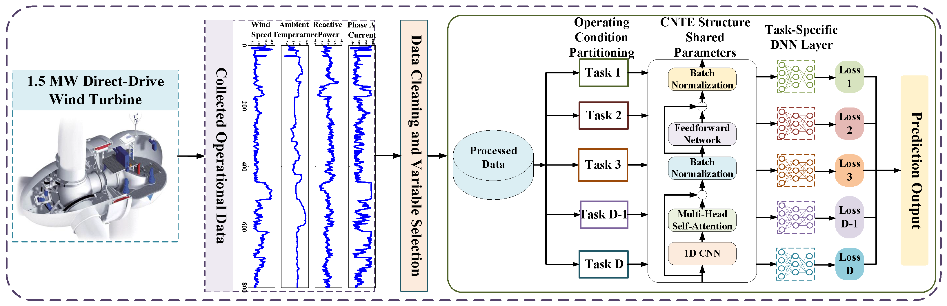
To address the problems of strong non-stationarity in wind power sequences and insufficient forecasting stability of a single model under meteorology-driven operating condition variations, this paper proposes a wind power forecasting method based on a Convolutional Normalized Transformer Encoder and Multi-Task Learning, termed CNTE-MTL; its overall framework is illustrated in Figure 1. First, a 1.5 MW direct-drive wind turbine is taken as the research object, and SCADA operational data, including wind speed, wind direction, ambient temperature, reactive power, and active power, are collected. High-quality modeling samples are then constructed through data cleaning, outlier removal, and key variable selection. Second, the samples are partitioned into different operating conditions according to meteorological variables and operational characteristics, and the power forecasting tasks under different meteorology-driven operating conditions are regarded as multiple correlated subtasks. Subsequently, within the multi-task learning framework, a CNTE-based shared feature extraction network is employed to provide a unified representation of samples from different operating conditions. Specifically, one-dimensional convolution is used to extract local temporal fluctuation features, while a Transformer encoder is incorporated to model long-term dependency relationships, thereby enabling cross-condition information sharing and collaborative modeling. On the basis of the shared representations, corresponding task-specific prediction layers are configured for different operating conditions, and the entire model is optimized through a joint loss function to finally generate the wind power forecasting results. The specific design details are presented as follows:

2.1. Data Preprocessing and Operating Condition Partitioning

The data collected by wind turbine SCADA systems are characterized by high variable dimensionality, complex operating environments, evident measurement noise, and frequent switching of operating states. Raw data usually contain missing values, outliers, and redundant variables. If the raw data are directly used for model training, the learning of model parameters may be disturbed by abnormal observations, thereby reducing forecasting accuracy and stability [26]. Therefore, before modeling, SCADA data need to be cleaned, normalized, screened for relevant variables, and divided into operating conditions so as to construct a high-quality sample set that satisfies the requirements of model training.

To ensure the reproducibility and rigor of the time-series forecasting task, the data processing procedure in this paper was carried out in the following order: raw SCADA data acquisition; missing-value statistics and handling; outlier identification and removal; chronological division of the training, validation, and test sets; normalization; mRMR-based variable selection; meteorology-driven operating condition division; sliding-window sample construction; and multi-task model training. It should be particularly noted that, in order to avoid data leakage, all steps involving statistical parameter estimation were performed only on the training set. For example, the maximum and minimum values required for normalization, the mean and standard deviation used in the 3$\sigma$ criterion, the mRMR-based variable selection results, and the K-means cluster centers were all determined from the training set. The validation and test sets were transformed and assigned only using the parameters obtained during the training stage, and they did not participate in the estimation of preprocessing parameters.

(1)

Data Cleaning and Normalization

Let the raw SCADA data be expressed as

$$\mathbf{X}=\left\{x_{i,t}\mid i=1,2,\cdots ,M; t=1,2,\cdots ,T\right\},$$

(1)

where M denotes the number of monitored variables, T denotes the length of the time series, and $x_{i,t}$ represents the observed value of the i-th variable at time t.

For missing data, this paper adopts linear interpolation based on adjacent valid samples:

$$x_{i,t}=x_{i,t_1}+{\displaystyle \frac{t-t_1}{t_2-t_1}}\left(x_{i,t_2}-x_{i,t_1}\right),$$

(2)

where $t_1$ and $t_2$ denote the nearest valid observation times before and after the missing time t, respectively. Linear interpolation is adopted because the SCADA data used in this paper have a fixed sampling interval of 10 min. For continuous monitoring of variables such as wind speed, temperature, rotational speed, current, and power, when missing values occur only as short-term, sporadic, and isolated omissions, strong temporal continuity usually exists between adjacent time points. Linear interpolation can preserve the integrity of the time series without significantly altering local variation trends, and it can also avoid sliding-window discontinuities caused by directly deleting samples.

Meanwhile, linear interpolation is not applicable to all missing-data cases. For data segments with long continuous missing intervals, variable variation trends that cannot be reasonably estimated within the missing interval, or data that obviously do not satisfy the assumption of local continuity, this paper does not apply simple interpolation for completion. Instead, such segments are removed during data cleaning or excluded from subsequent model training. This strategy reduces the risk that interpolation results over long missing intervals may deviate from the true operating state.

To reduce the influence of sensor anomalies, communication failures, recording errors, and abnormal turbine operating states on model training, this paper adopts the 3$\sigma$ criterion to preliminarily identify obvious abnormal samples:

$$\left|x_{i,t}-{\mu }_i\right|>3{\sigma }_i,$$

(3)

where ${\mu }_i$ and ${\sigma }_i$ denote the mean and standard deviation of the i-th variable in the training set, respectively. The 3$\sigma$ criterion is intuitive, interpretable, and easy to implement, making it suitable for preliminary screening of extreme measurement points in SCADA data that clearly deviate from the normal fluctuation range. It should be noted that the 3$\sigma$ criterion is not intended to identify all complex operating condition variations, nor does it regard normal meteorological fluctuations, operating condition switching, or power changes as anomalies. In this paper, it is used only to remove extreme outliers that clearly violate variable measurement patterns or the distribution characteristics of operating data. Samples corresponding to normal meteorological disturbances and operating condition variations are retained for subsequent operating condition division and multi-task forecasting modeling.

After missing-value handling and outlier removal, Min–Max normalization is used to standardize the input variables in order to eliminate the influence of differences in physical units and numerical ranges among variables on model training:

$${\tilde{x}}_{i,t}={\displaystyle \frac{x_{i,t}-x_i^{\min }}{x_i^{\max }-x_i^{\min }}},$$

(4)

where $x_i^{\max }$ and $x_i^{\min }$ denote the maximum and minimum values of the i-th variable in the training set, respectively. The validation and test sets are normalized using the maximum and minimum values obtained from the training set, thereby preventing information from the validation and test sets from being introduced into the model training process in advance.

(2)

Variable Selection Based on mRMR

Wind turbine SCADA systems typically record a large number of operating variables, including meteorological variables, mechanical state variables, electrical state variables, and control state variables. Directly feeding all variables into the forecasting model would not only increase computational complexity but might also introduce redundant information and noisy variables, thereby reducing the training efficiency and forecasting stability. Therefore, this paper adopts the Minimum Redundancy Maximum Relevance (mRMR) method for variable selection, aiming to obtain a subset of variables that are highly correlated with wind power while exhibiting low redundancy among themselves.

Let the candidate feature set be defined as

$$F=\left\{f_1,f_2,⃯,f_n\right\},$$

(5)

and let the target variable be wind power y. First, mutual information is used to measure the relevance between each candidate feature and the target variable:

$$D(f_i,y)=I(f_i;y),$$

(6)

where mutual information is defined as

$$I(f_i;y)=\sum _{f_i}\sum _{y}p(f_i,y)\log {\displaystyle \frac{p(f_i,y)}{p\left(f_i\right)p\left(y\right)}}.$$

(7)

To reduce information redundancy among features, the average redundancy term is introduced:

$$R\left(f_i\right)={\displaystyle \frac{1}{\left|S\right|}}\sum _{f_j\in S}I(f_i;f_j),$$

(8)

where S denotes the set of variables that have already been selected into the feature subset. Finally, features are selected according to the following criterion:

$$\max J\left(f_i\right)=D(f_i,y)-R\left(f_i\right).$$

(9)

Through the above procedure, information redundancy among variables can be reduced while ensuring strong relevance between the input variables and wind power, thereby improving model training efficiency and forecasting stability.

It should be particularly noted that this paper distinguishes between “meteorological variables used for operating condition division” and “model input variables used for power forecasting”. Meteorological variables such as wind speed, wind direction, and ambient temperature are mainly used to characterize changes in external meteorological conditions and generate operating condition labels. In contrast, the input variables ultimately fed into the CNTE-MTL forecasting model are multidimensional SCADA variables selected by mRMR, including not only meteorological variables but also variables reflecting the mechanical and electrical operating states of the turbine, such as generator speed, rotor speed, pitch motor current, converter current, phase current, and power factor. Therefore, this paper does not rely solely on meteorological data for wind power forecasting; instead, based on meteorology-driven operating condition division, it comprehensively utilizes both turbine operating state variables and external meteorological variables to characterize the nonlinear relationship among “meteorological driving factors, turbine response, and power output”.

(3)

Meteorology-Driven Operating Condition Division

The operating state of wind turbines is closely related to external meteorological conditions. Wind speed directly determines the intensity of wind energy input and is a key factor affecting wind power output. Wind direction influences the inflow direction, yaw response, and effective wind energy capture capability of the turbine. Ambient temperature affects air density, the thermal state of the turbine, and certain mechanical and electrical operating characteristics. Therefore, this paper selects wind speed $v_t$, wind direction ${\theta }_t$, and ambient temperature $T_t$ to construct the meteorological feature vector:

$${\mathbf{z}}_t={\left[v_t,{\theta }_t,T_t\right]}^T.$$

(10)

K-means clustering is then adopted to perform meteorology-driven operating condition division for the operating samples. Meteorological variables, rather than target-related variables such as active power, are selected for clustering mainly to identify different operating patterns from the perspective of external environmental driving factors, thereby avoiding the direct introduction of prediction target information into the operating condition division process, and reducing the risk of potential information leakage.

The optimization objective of K-means clustering is expressed as

$$\min {\displaystyle \sum _{k=1}^K}\sum _{{\mathbf{z}}_t\in C_k}{∥{\mathbf{z}}_t-{\mathit{\mu }}_k∥}^2,$$

(11)

where K denotes the number of operating condition categories, $C_k$ represents the sample set of the k-th category, and ${\mathit{\mu }}_k$ denotes the cluster center of the k-th category. The cluster centers are iteratively updated as follows:

$${\mathit{\mu }}_k={\displaystyle \frac{1}{|C_k|}}\sum _{{\mathbf{z}}_t\in C_k}{\mathbf{z}}_t.$$

(12)

After operating condition division is completed, a dataset with operating condition labels is constructed as follows:

$$D={\left\{\left({\mathbf{x}}_t,y_t,c_t\right)\right\}}_{t=1}^T,$$

(13)

where ${\mathbf{x}}_t$ denotes the model input features after variable selection, $y_t$ denotes wind power, and $c_t\in \{1,2,\cdots ,K\}$ denotes the meteorology-driven operating condition category corresponding to the sample. This dataset serves as the input basis for the subsequent CNTE-MTL multi-task forecasting model.

(4)

Selection of the Number of Clusters and Description of Operating Condition Sample Distribution

The selection of the number of clusters K directly affects the results of operating condition division and the subsequent performance of multi-task forecasting modeling. When K is too small, different meteorological operating patterns may be merged into the same condition, resulting in large intra-condition differences and making it difficult to fully characterize the differences in power evolution under varying meteorological conditions. When K is too large, although the operating condition division becomes more detailed, the number of samples in some conditions may be significantly reduced, which can easily lead to sample imbalance in multi-task training and increase model complexity and the risk of overfitting. Therefore, the selection of K requires a trade-off among condition separability, sample size balance, and subsequent forecasting stability.

To evaluate the effectiveness of operating condition division under different numbers of clusters, this paper adopts the Silhouette coefficient and the Davies–Bouldin index for comprehensive assessment. The Silhouette coefficient measures the intra-cluster compactness and inter-cluster separation of samples, with a larger value indicating better clustering performance. The Davies–Bouldin index measures the similarity between different clusters, with a smaller value indicating a better clustering result. The Silhouette coefficient is defined as

$$S\left(i\right)={\displaystyle \frac{b\left(i\right)-a\left(i\right)}{\max \left\{a\right(i),b(i\left)\right\}}},$$

(14)

where $a\left(i\right)$ denotes the average distance between sample i and other samples within the same cluster, and $b\left(i\right)$ denotes the average distance between sample i and the samples in the nearest neighboring cluster. The Davies–Bouldin index is defined as

$$DB={\displaystyle \frac{1}{K}}{\displaystyle \sum _{i=1}^K}\underset{j\ne i}{\max }\left({\displaystyle \frac{{\sigma }_i+{\sigma }_j}{d({\mathbf{c}}_i,{\mathbf{c}}_j)}}\right),$$

(15)

where ${\sigma }_i$ and ${\sigma }_j$ denote the average distances from samples in the i-th and j-th clusters to their respective cluster centers, and $d({\mathbf{c}}_i,{\mathbf{c}}_j)$ denotes the distance between the cluster centers of the i-th and j-th clusters.

In the specific experiments, we conducted a sensitivity analysis of the clustering results for $K=2\sim 9$ and determined the final number of operating conditions by comprehensively considering the Silhouette coefficient, Davies–Bouldin index, sample proportion of each condition, and subsequent forecasting performance. To prevent severe imbalance in operating condition sample sizes from affecting multi-task training, the number and proportion of samples for each condition in the training, validation, and test sets was also counted, and condition-specific forecasting performance is reported in the experiment section. If the number of samples in certain conditions is significantly small, the task weights of minority-condition tasks can be appropriately increased in the multi-task loss, or strategies such as balanced sampling and sample reweighting can be adopted to reduce the dominance of majority conditions in model training.

2.2. Multi-Task Learning Method Based on CNTE

To address the distribution shift in power forecasting caused by rapid meteorology-driven operating condition changes, this paper models wind power forecasting under different meteorological conditions as a set of interrelated learning tasks, and it introduces a multi-task learning framework to enable cross-condition information sharing and collaborative modeling. Let the set of operating conditions obtained through condition division be defined as

$$C=\left\{1,2,\cdots ,K\right\}.$$

For any time instant t, a sliding-window input sequence with length L is constructed as follows:

$${\mathbf{X}}_t=\left[{\mathbf{x}}_{t-L+1},{\mathbf{x}}_{t-L+2},\cdots ,{\mathbf{x}}_t\right]\in {\mathbb{R}}^{L\times d},$$

(16)

where L denotes the sliding-window length, d denotes the input variable dimension, and ${\mathbf{x}}_t$ represents the multidimensional SCADA input features at time t. The corresponding prediction target is $y_t$, and the operating condition label is $c_t\in C$. Since the SCADA data are sampled at a 10 min interval, when $L=12$, the model uses the historical operating states over approximately 120 min before the current time instant for power forecasting. This setting enables the model to make predictions not only based on instantaneous meteorological variables but also by incorporating meteorological variation trends and turbine operating dynamics over the preceding period, thereby more reasonably characterizing the influence of historical states on the current power output.

This paper adopts a multi-task structure consisting of a shared feature extractor and condition-specific prediction heads. The shared component is used to learn common temporal representations across different operating conditions, while the condition-specific component is used to characterize the differences in power evolution under each condition. For a sample ${\mathbf{X}}_t$, the model first obtains a unified feature representation through the shared CNTE network. Then, according to its operating condition label $c_t$, this feature representation is fed into the corresponding condition-specific prediction head to obtain the wind power forecasting value. In this way, the model can achieve common information sharing across operating conditions while preserving differentiated forecasting patterns under different meteorological conditions.

(1)

CNTE Shared Feature Extraction Network

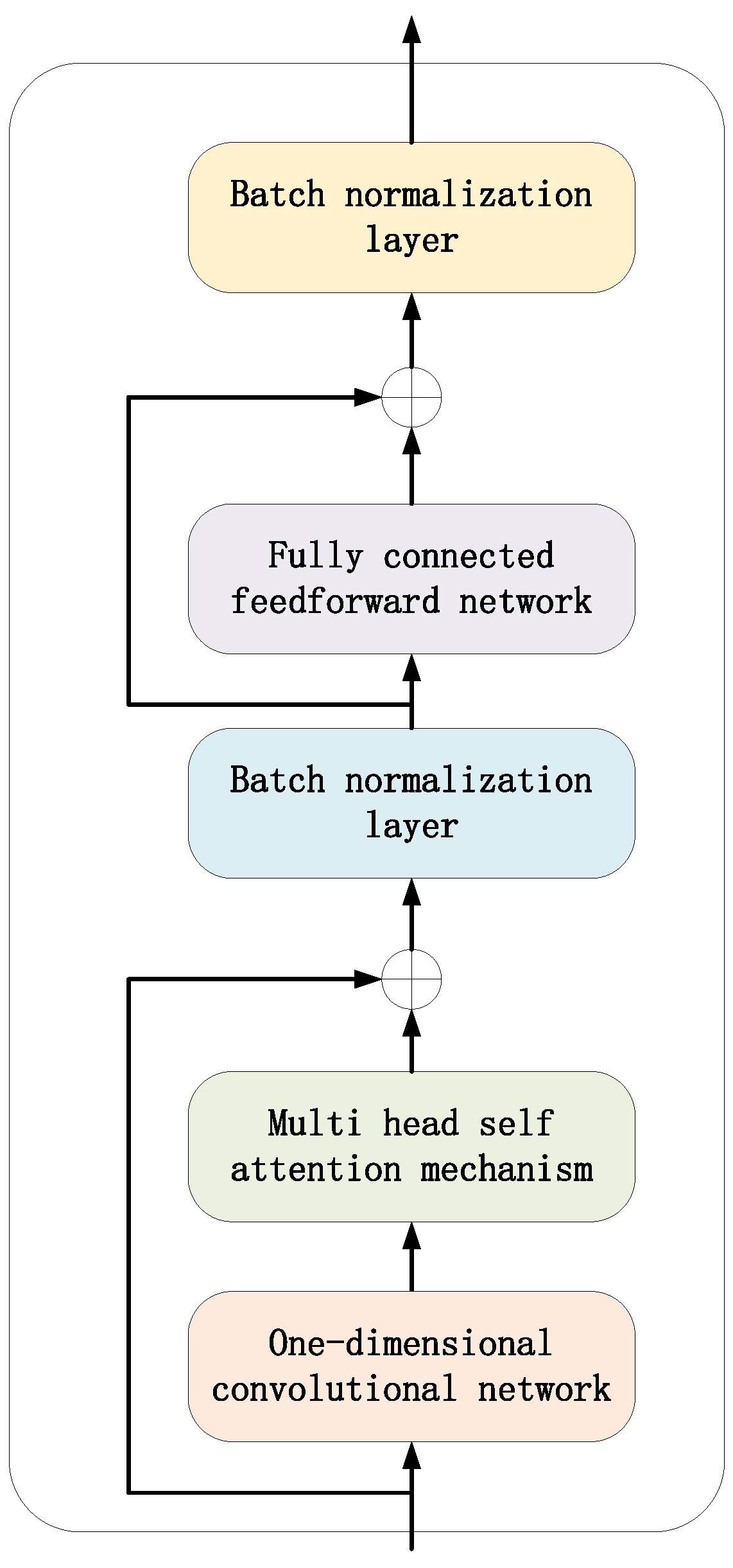
Wind power SCADA sequences are typically characterized by pronounced local fluctuations, frequent short-term disturbances, complex long-term dependencies, and large differences in variable scales. If a standard Transformer encoder is directly used for feature extraction, it may suffer from insufficient capture of local temporal patterns and sensitivity to data-scale variations during training. Therefore, we constructed a Convolutional Normalized Transformer Encoder (CNTE) as the shared feature extraction network. The CNTE consists of a one-dimensional convolutional layer, a multi-head self-attention layer, a feed-forward network, residual connections, and batch normalization layers, as shown in Figure 2. Specifically, one-dimensional convolution is used to extract local temporal fluctuation features, multi-head self-attention is used to capture long-term dependencies among different time steps within the historical window, and batch normalization together with residual connections is employed to improve training stability.

①

One-Dimensional Convolution for Local Feature Extraction.

For the input sequence ${\mathbf{X}}_t\in {\mathbb{R}}^{L\times d}$, a one-dimensional convolutional transformation is performed to obtain the local temporal representation:

$${\mathbf{H}}_0=\varphi \left(\mathrm{Conv}1\mathrm{D}\left({\mathbf{X}}_t;{\mathbf{W}}_c,{\mathbf{b}}_c\right)\right),$$

(17)

where ${\mathbf{W}}_c$ and ${\mathbf{b}}_c$ denote the convolution kernel parameters and bias term, respectively; $\varphi (·)$ denotes the nonlinear activation function; ${\mathbf{H}}_0\in {\mathbb{R}}^{L\times d_m}$ denotes the convolved feature representation; and $d_m$ denotes the hidden feature dimension.

②

Multi-Head Self-Attention for Long-Term Dependency Modeling.

Based on the convolutional representation, a multi-head self-attention mechanism is adopted to capture dependencies among different time steps:

$$\mathbf{Q}={\mathbf{H}}_0{\mathbf{W}}^Q, \mathbf{K}={\mathbf{H}}_0{\mathbf{W}}^K, \mathbf{V}={\mathbf{H}}_0{\mathbf{W}}^V,$$

(18)

$$\mathrm{Attn}(\mathbf{Q},\mathbf{K},\mathbf{V})=\mathrm{softmax}\left({\displaystyle \frac{\mathbf{Q}{\mathbf{K}}^T}{\sqrt{d_k}}}\right)\mathbf{V},$$

(19)

$$\mathrm{MHSA}\left({\mathbf{H}}_0\right)=\mathrm{Concat}\left({\mathrm{head}}_1,\cdots ,{\mathrm{head}}_h\right){\mathbf{W}}^O,$$

(20)

where ${\mathbf{W}}^Q$, ${\mathbf{W}}^K$, ${\mathbf{W}}^V$, and ${\mathbf{W}}^O$ are projection matrices, h denotes the number of attention heads, $d_k$ denotes the dimension of the key vector in each head, and ${\mathrm{head}}_i=\mathrm{Attn}({\mathbf{Q}}_i,{\mathbf{K}}_i,{\mathbf{V}}_i)$. Combined with residual connection and batch normalization, the output of the attention sublayer is expressed as

$${\mathbf{H}}_1=\mathrm{BN}\left({\mathbf{H}}_0+\mathrm{MHSA}\left({\mathbf{H}}_0\right)\right).$$

(21)

③

Feed-Forward Network for Enhanced Nonlinear Representation.

After long-term dependency modeling, a two-layer fully connected feed-forward network is introduced for nonlinear mapping:

$$\mathrm{FFN}\left({\mathbf{H}}_1\right)=\sigma \left({\mathbf{H}}_1{\mathbf{W}}_1+{\mathbf{b}}_1\right){\mathbf{W}}_2+{\mathbf{b}}_2,$$

(22)

where ${\mathbf{W}}_1$, ${\mathbf{W}}_2$, ${\mathbf{b}}_1$, and ${\mathbf{b}}_2$ are the parameters of the feed-forward network, and $\sigma (·)$ denotes the activation function. Combined with residual connection and batch normalization, the output of the encoding block is obtained as follows:

$${\mathbf{H}}_2=\mathrm{BN}\left({\mathbf{H}}_1+\mathrm{FFN}\left({\mathbf{H}}_1\right)\right).$$

(23)

The above CNTE encoding block can be stacked for N layers to form the shared feature extractor $f_{\theta }(·)$, thereby obtaining the high-level temporal representation:

$${\mathbf{Z}}_t=f_{\theta }\left({\mathbf{X}}_t\right).$$

(24)

For power forecasting, temporal pooling can be applied to ${\mathbf{Z}}_t$ to obtain the sample-level shared representation:

$${\mathbf{z}}_t={\displaystyle \frac{1}{L}}{\displaystyle \sum _{\ell =1}^L}{\mathbf{Z}}_{t,\ell },$$

(25)

where ${\mathbf{z}}_t\in {\mathbb{R}}^{d_m}$ denotes the shared temporal feature representation of sample ${\mathbf{X}}_t$.

(2)

Condition-Specific Prediction Heads and Sample Routing Mechanism

After obtaining the shared representation ${\mathbf{z}}_t$, this paper assigns an independent condition-specific prediction head $g_{{\phi }_k}(·)$ to each operating condition task $k\in C$. For a sample with the condition label $c_t=k$, the prediction result is given by

$${\widehat{y}}_t=g_{{\phi }_k}\left({\mathbf{z}}_t\right), c_t=k,$$

(26)

where ${\phi }_k$ denotes the parameters of the prediction head for the k-th operating condition. Accordingly, the sample routing process of CNTE-MTL consists of two stages: First, samples from all operating conditions are fed into the shared CNTE network to obtain unified temporal feature representations. Second, according to the condition label $c_t$, the model routes the shared representation to the corresponding condition-specific prediction head. In this way, differentiated prediction mappings can be established for different meteorological conditions while sharing common cross-condition knowledge.

During offline training, the condition labels are determined by the K-means clustering results obtained from the training set [27]. For validation, test, or future online prediction samples, the clustering model is not retrained; instead, each sample is assigned to the nearest operating condition category according to the distance between its meteorological features and the cluster centers obtained during training:

$$c_t=\arg \underset{k}{\min }{∥{\mathbf{z}}_t^m-{\mathit{\mu }}_k∥}^2,$$

(27)

where ${\mathbf{z}}_t^m={\left[v_t,{\theta }_t,T_t\right]}^T$ denotes the meteorological feature vector at time t, and ${\mathit{\mu }}_k$ denotes the cluster center of the k-th meteorological condition obtained during training.

(3)

Multi-Task Loss Function and Sample Imbalance Handling

This paper adopts the Mean Square Error as the prediction loss for each individual operating condition task. For the k-th operating condition task, let its sample set be $D_k$, and the corresponding loss is defined as

$${\mathcal{L}}_k={\displaystyle \frac{1}{|D_k|}}\sum _{({\mathbf{X}}_t,y_t)\in D_k}{\left(y_t-{\widehat{y}}_t\right)}^2,$$

(28)

where $|D_k|$ denotes the number of samples in the k-th operating condition task. It should be noted that this paper first averages the sample errors within each operating condition task, rather than directly summing the errors over all samples from all conditions. This design prevents operating conditions with larger sample sizes from dominating the total loss merely because of their larger sample proportions.

The overall objective function of multi-task learning is defined as the weighted sum of the losses of all operating conditions:

$$\mathcal{L}={\displaystyle \sum _{k=1}^K}{\lambda }_k{\mathcal{L}}_k,$$

(29)

where ${\lambda }_k$ denotes the loss weight of the k-th operating condition task, which is used to balance the influence of sample size differences among different conditions on the training process. When the sample sizes of different conditions are relatively balanced, ${\lambda }_k=1/K$ can be adopted. When some operating conditions contain significantly fewer samples, the weights of minority-condition tasks can be appropriately increased to reduce the risk that the model becomes overly biased toward majority conditions. In practical applications, ${\lambda }_k$ can also be adjusted according to condition-specific sample proportions, validation errors, or task uncertainty.

For real wind farms, meteorological conditions are often unevenly distributed. Conventional stable operating conditions usually account for a large number of samples, whereas strong wind, rapid wind direction changes, high temperatures, low temperatures, or other extreme meteorological conditions often contain fewer samples. However, minority conditions are often of high engineering importance. Therefore, in the experimental section, this paper further reports the number and proportion of samples for each operating condition in the training, validation, and test sets, and it presents prediction error metrics under different conditions, so as to prevent the overall evaluation metrics from masking performance variations under minority conditions. For operating conditions with severely insufficient samples, future work may further incorporate sample reweighting, oversampling, data augmentation, or transfer learning methods to improve forecasting reliability under minority yet critical conditions.

(4)

Boundary Samples Between Operating Conditions and Prediction Output Smoothing Strategy

In practical online forecasting scenarios, meteorological variables such as wind speed, wind direction, and ambient temperature may fluctuate frequently near the boundary between two operating conditions. If hard condition labels are directly used for sample routing, samples may switch frequently between two adjacent condition-specific prediction heads, which may lead to the risk of local jumps in the predicted values. To address this issue, this paper provides an explanation from two perspectives: model structure, and boundary sample handling.

First, CNTE-MTL does not train a completely independent prediction model for each operating condition. Instead, different condition tasks share the same CNTE feature extraction network, and only the final prediction heads contain condition-specific parameters. Therefore, even if samples switch between adjacent operating conditions, their underlying temporal representations are still extracted by the same shared network. This helps preserve common cross-condition information and, to some extent, alleviates prediction discontinuities caused by operating condition switching.

Second, for samples located near the boundary between two operating conditions, a distance-weighted fusion strategy can be adopted to further smooth the prediction output. Let the distance between the sample ${\mathbf{z}}_t^m$ and the k-th cluster center be defined as

$$d_{t,k}=∥{\mathbf{z}}_t^m-{\mathit{\mu }}_k∥.$$

(30)

Then, soft weights can be constructed according to the distances:

$${\alpha }_{t,k}={\displaystyle \frac{\exp \left(-d_{t,k}\right)}{{\sum }_{j=1}^K\exp \left(-d_{t,j}\right)}}.$$

(31)

The outputs of multiple condition-specific prediction heads are then weighted and fused as follows:

$${\widehat{y}}_t={\displaystyle \sum _{k=1}^K}{\alpha }_{t,k}{g}_{{\phi }_k}\left({\mathbf{z}}_t\right).$$

(32)

When a sample clearly belongs to a certain operating condition, the corresponding weight approaches 1, and the model output is mainly determined by the prediction head of that condition. When a sample is located near the boundary between two operating conditions, adjacent condition-specific prediction heads jointly participate in prediction, allowing the output to transition gradually with changes in meteorological conditions, and reducing the possibility of abrupt changes caused by hard switching.

In addition to distance-weighted fusion, sliding temporal-window smoothing or a condition-switching hysteresis mechanism can also be introduced in practical online deployment. That is, the task head is switched only when the sample remains stably within the new operating condition region for several consecutive time steps, thereby avoiding frequent switching caused by instantaneous meteorological disturbances. The overall procedure of the proposed CNTE-MTL method is summarized in Algorithm 1.

Algorithm 1 Multi-task wind power forecasting method based on CNTE-MTL.

Input:  Raw SCADA data $\mathbf{X}$, target power sequence y, number of operating conditions K, sliding-window length L, number of training epochs E, learning rate $\eta$; Output:  Trained shared CNTE feature extractor parameters $\theta$ and condition-specific prediction head parameters ${\left\{{\phi }_k\right\}}_{k=1}^K$;   1: Handle missing values and remove outliers from the raw SCADA data;   2: Divide the training, validation, and test sets in chronological order;   3: Estimate normalization parameters using only the training set, and normalize the training, validation, and test sets;   4: Select key input variables using the mRMR method based only on the training set;   5: Train the K-means clustering model using the meteorological variables ${\mathbf{z}}_t^m={[v_t,{\theta }_t,T_t]}^T$ in the training set, and obtain the cluster centers ${\left\{{\mathit{\mu }}_k\right\}}_{k=1}^K$;   6: Generate operating condition labels for the training samples; assign condition labels to the validation and test samples according to their distances to the cluster centers obtained from the training set;   7: Construct the time-series sample set with operating condition labels according to the sliding-window length L, denoted as $D=\left\{({\mathbf{X}}_t,y_t,c_t)\right\}$;   8: Initialize the shared CNTE feature extractor $f_{\theta }(·)$ and the condition-specific prediction heads ${\left\{g_{{\phi }_k}(·)\right\}}_{k=1}^K$;   9: for $e=1$ to E do 10:      Divide the training samples into K condition-specific subsets ${\left\{D_k\right\}}_{k=1}^K$ according to their operating condition labels; 11:      for $k=1$ to K do 12:           Feed the samples ${\mathbf{X}}_t\in D_k$ under operating condition k into the shared CNTE network to obtain the shared representation: $${\mathbf{z}}_t=f_{\theta }\left({\mathbf{X}}_t\right)$$ 13:           Feed the shared representation into the k-th condition-specific prediction head to obtain the prediction result: $${\widehat{y}}_t=g_{{\phi }_k}\left({\mathbf{z}}_t\right)$$ 14:           Calculate the prediction loss of the k-th operating condition task: $${\mathcal{L}}_k={\displaystyle \frac{1}{|D_k|}}\sum _{({\mathbf{X}}_t,y_t)\in D_k}{\left(y_t-{\widehat{y}}_t\right)}^2$$ 15:      end for 16:      Set the task weight ${\lambda }_k$ according to the sample size or validation error of each operating condition, and calculate the total loss: $$\mathcal{L}={\displaystyle \sum _{k=1}^K}{\lambda }_k{\mathcal{L}}_k$$ 17:      Update the shared parameters $\theta$ and the condition-specific prediction head parameters ${\left\{{\phi }_k\right\}}_{k=1}^K$ through backpropagation and the optimizer with learning rate $\eta$; 18: end for 19: Output the trained CNTE-MTL model.

3. Comparative Experiments and Result Analysis

3.1. Data Source and Preprocessing

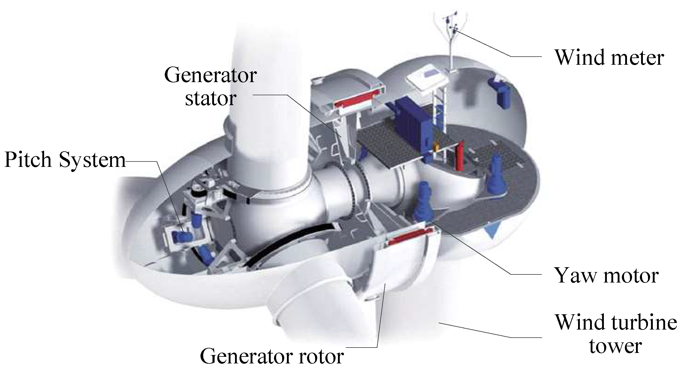
The experimental data used in this paper were obtained from actual operational SCADA monitoring data collected from a wind farm in northern China. The research object is a direct-drive wind turbine with a rated capacity of 1.5 MW, whose structural schematic is shown in Figure 3. The turbine mainly consists of a rotor system, generator system, pitch system, yaw system, and tower structure. The rotor is directly coupled with a permanent-magnet synchronous generator, enabling efficient conversion of wind energy into electrical energy. Meteorological monitoring devices, such as an anemometer and a wind vane, are installed on the top of the turbine to acquire external meteorological information, including ambient wind speed and wind direction, in real time.

The SCADA system records turbine operating states and environmental meteorological information at a sampling interval of 10 min. The raw monitoring variables include multidimensional operational data such as wind speed, wind direction, ambient temperature, turbine rotational speed, generator temperature, current, power factor, and output power. The collected data span from January 2024 to March 2024, comprising 12,960 operational records and 93 raw monitoring variables. It should be noted that the data used in this paper mainly cover the period from winter to early spring and, therefore, cannot fully represent the multi-seasonal operating characteristics throughout the whole year. Accordingly, the experimental results in this paper are mainly used to verify the effectiveness of the proposed CNTE-MTL method within the current data range. The generalization capability of the model under year-round operating conditions, high-temperature conditions, typhoon events, and other extreme weather scenarios still requires further validation using data over a longer time span and more extreme-weather samples.

Since the SCADA data used in this paper were obtained from an actual wind farm operation system, they involve wind farm production and operation information as well as enterprise data security requirements; therefore, the raw data cannot be publicly released. To improve research transparency, this paper additionally provides the sampling interval, time range, number of raw samples, number of variables, proportion of missing data, proportion of abnormal samples, and statistical characteristics of the selected variables, without disclosing sensitive enterprise information. Partially anonymized statistical information and experimental settings can be made available upon reasonable request. The basic information of the dataset is shown in

Table 1. Basic information of the SCADA dataset.

Item	Description
Data source	SCADA monitoring data from a wind farm in northern China
Turbine type	1.5 MW direct-drive wind turbine
Sampling interval	10 min
Data time range	January 2024 to March 2024
Number of raw operational records	12,960
Number of raw monitoring variables	93
Prediction target	Active power
Dataset division method	Chronological division
Training/validation/test set ratio	3:1:1

.

Due to the complex on-site operating environment, SCADA data may be affected during acquisition by communication failures, sensor errors, turbine start-up and shutdown, power curtailment operation, and abnormal operating states. As a result, the raw data inevitably contain missing values, outliers, and noisy observations. Directly using these data for model training may cause the model to be disturbed by abnormal measurements, thereby reducing the forecasting stability; therefore, data cleaning is required before model training.

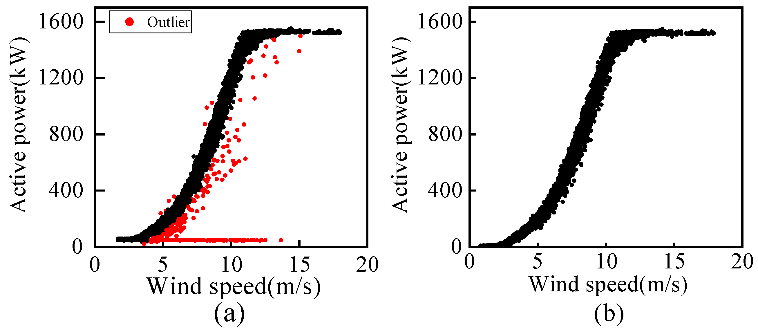
In this paper, the missing status of each variable is first analyzed. Short-term and sporadic missing values are completed using linear interpolation. For data segments with long continuous missing intervals or those that clearly do not satisfy the local continuity assumption, simple interpolation is not performed; instead, these segments are removed or excluded from model training. Subsequently, the 3$\sigma$ criterion is used to preliminarily identify abnormal observations that significantly deviate from the normal distribution range. In addition, samples that clearly violate the normal operating characteristics of wind turbines are removed according to the wind speed–power scatter distribution. To more clearly illustrate the quality of the raw data and the influence of the data-cleaning process on the sample size, the statistics of missing data and abnormal samples are supplemented, as shown in

Table 2. Statistics of missing values and abnormal samples.

Data Processing Item	Number of Records	Proportion/%
Raw operational records	12,960	100.00
Records containing missing values	286	2.21
Records completed by linear interpolation	214	1.65
Records removed due to continuous missing values	72	0.56
Abnormal records identified by the 3$\sigma$ criterion	391	3.02
Abnormal records based on the wind speed–power relationship	254	1.96
Valid records after cleaning	12,232	94.38

.

To intuitively demonstrate the effectiveness of data cleaning, Figure 4 presents the scatter distribution between wind speed and wind power. As shown in Figure 4a, before data cleaning, there are many abnormal samples in the wind speed–power scatterplot that deviate from the normal power curve, such as samples with obviously low power at the same wind speed, zero power, or values deviating from the normal power curve. These abnormal points mainly originate from turbine start-up and shutdown processes, communication errors, power curtailment operation, and certain sensor measurement anomalies, which lead to obvious dispersion of power data under the same wind speed condition. After data cleaning, as shown in Figure 4b, the obvious abnormal samples are effectively removed, and the relationship between wind speed and power exhibits a clearer power curve distribution. The overall data distribution becomes more concentrated and is consistent with the typical wind speed–power characteristics of wind turbines.

After data cleaning, all input variables are normalized to eliminate the influence of dimensional differences among variables on model training, mapping them into a unified numerical range and thereby improving the stability and convergence speed of the training process. To avoid data leakage in the time-series forecasting task, the training, validation, and test sets are divided in chronological order. Statistical parameters required for normalization, such as the maximum and minimum values, are calculated only based on the training set and then applied to the validation and test sets. Similarly, mRMR-based variable selection and K-means cluster centers are determined only from the training set, while the validation and test sets do not participate in the estimation of these parameters.

3.2. Variable Selection and Operating Condition Partitioning

Since the wind turbine SCADA system monitors a large number of variables, the raw data include 93 operational variables, among which strong correlations and information redundancy often exist. Directly feeding all variables into the forecasting model would not only increase the training complexity but might also introduce redundant information and noisy variables, thereby reducing the forecasting accuracy and stability. Therefore, this paper adopts the Minimum Redundancy Maximum Relevance (mRMR) method to screen the raw variables and select key variables that are closely related to wind power forecasting and have low redundancy as the subsequent model inputs [28]. After mRMR-based screening, 10 key variables were finally selected, as shown in

Table 3. Final selected key variables of the wind turbine.

No.	Variable Name	Unit	No.	Variable Name	Unit
1	Historical active power	kW	6	Wind speed	m/s
2	Generator speed	r/min	7	Rotor speed 2	r/min
3	Ambient temperature	°C	8	Power factor	–
4	Grid-side current of converter	A	9	Phase-A current	A
5	No. 3 pitch motor current	A	10	Converter motor speed	r/min

.

As shown in Table 3, the selected variables mainly cover the meteorological conditions, mechanical operating states, and electrical output characteristics of the turbine. Among them, wind speed and ambient temperature can characterize changes in the external meteorological environment; generator speed, rotor speed, and pitch motor current can reflect the mechanical operating state of the turbine; and grid-side converter current, Phase-A current, power factor, and active power can describe the electrical output characteristics of the turbine. These variables reflect the intrinsic relationship between wind turbine operating states and power variations from different perspectives, providing sufficient input information for subsequent wind power forecasting modeling.

It should be emphasized that this paper does not rely solely on meteorological data for power forecasting. Meteorological variables are mainly used for operating condition division to characterize differences in operating patterns driven by external meteorological conditions. In contrast, the input variables finally fed into the CNTE-MTL forecasting model are multidimensional SCADA variables selected by mRMR, including not only meteorological information such as wind speed and ambient temperature but also variables reflecting the mechanical and electrical operating states of the wind turbine, such as generator speed, rotor speed, pitch motor current, converter current, phase current, and power factor. In this way, the model can simultaneously consider the effects of “meteorological driving factors” and “the turbine’s dynamic response” on power output, thereby more comprehensively characterizing the variation patterns of wind power.

To further improve the transparency and reproducibility of the data description, this paper additionally provides the statistical characteristics of the selected variables, including the minimum value, maximum value, mean value, standard deviation, and missing-data proportion, as shown in

Table 4. Statistical characteristics of the selected variables.

Variable Name	Unit	Minimum	Maximum	Mean	Standard Deviation	Missing Proportion/%
Historical active power	kW	0.00	1506.80	641.25	508.63	1.76
Generator speed	r/min	0.00	18.47	10.52	4.21	1.38
Ambient temperature	°C	−18.60	9.80	−4.37	6.12	1.02
Grid-side current of converter	A	0.00	1248.30	540.76	411.28	1.64
No. 3 pitch motor current	A	−8.54	8.91	0.16	1.12	1.09
Wind speed	m/s	0.20	18.90	7.32	3.11	0.94
Rotor speed 2	r/min	0.00	18.45	10.49	4.20	1.41
Power factor	–	−0.15	1.00	0.94	0.08	1.57
Phase-A current	A	0.00	1241.70	533.62	405.74	1.69
Converter motor speed	r/min	0.00	1803.50	1052.84	438.31	1.33

.

After variable selection, K-means clustering is further adopted in this paper to perform meteorology-driven operating condition division, so as to characterize the differences in wind turbine operating states and power output patterns under different meteorological conditions. The variables used for operating condition division are wind speed, wind direction, and ambient temperature. These three meteorological variables were selected for the following reasons: wind speed directly determines the intensity of wind energy input and is the key meteorological factor affecting wind power output; wind direction affects the inflow direction, yaw state, and effective wind energy capture capability of the turbine; and ambient temperature influences air density, the thermal state of the turbine, and certain mechanical and electrical operating characteristics. Therefore, wind speed, wind direction, and ambient temperature can reflect typical operating condition differences from the perspective of external meteorological driving factors. Meanwhile, target-related variables such as active power are not directly used for clustering in this paper, in order to avoid introducing prediction target information into the operating condition division process in advance and causing potential information leakage.

To determine a reasonable number of clusters, this paper evaluates the clustering performance under different numbers of clusters using two metrics: the Silhouette coefficient and the Davies–Bouldin index [29]. The Silhouette coefficient measures the intra-cluster compactness and inter-cluster separation of samples, with a larger value indicating better clustering performance. The Davies–Bouldin index reflects the similarity between different clusters, with a smaller value indicating a better clustering result. Their expressions are given as follows:

$$S\left(i\right)={\displaystyle \frac{b\left(i\right)-a\left(i\right)}{\max \left\{a\right(i),b(i\left)\right\}}},$$

(33)

$$DB={\displaystyle \frac{1}{K}}{\displaystyle \sum _{i=1}^K}\underset{j\ne i}{\max }\left({\displaystyle \frac{{\sigma }_i+{\sigma }_j}{d({\mathbf{c}}_i,{\mathbf{c}}_j)}}\right),$$

(34)

where $a\left(i\right)$ denotes the average distance between sample i and other samples within the same cluster, and $b\left(i\right)$ denotes the average distance between sample i and the samples in the nearest neighboring cluster. K denotes the number of clusters; ${\sigma }_i$ and ${\sigma }_j$ denote the average distances from samples in the i-th and j-th clusters to their respective cluster centers; and $d({\mathbf{c}}_i,{\mathbf{c}}_j)$ denotes the distance between the cluster centers of the i-th and j-th clusters. The evaluation results under different numbers of clusters are shown in

Table 5. Clustering evaluation results for different numbers of clusters.

K	Silhouette Coefficient	Davies–Bouldin Index	K	Silhouette Coefficient	Davies–Bouldin Index
2	0.622851	0.578299	6	0.558212	0.603853
3	0.623634	0.508835	7	0.543037	0.594025
4	0.568615	0.562070	8	0.519613	0.649296
5	0.568079	0.588283	9	0.511770	0.663424

.

As shown in Table 5, when the number of clusters is 3, the Silhouette coefficient reaches its maximum value of 0.623634, while the Davies–Bouldin index reaches its minimum value of 0.508835, indicating that the clustering result has good intra-cluster compactness and inter-cluster separability. Therefore, the wind turbine operating samples are finally divided into three typical meteorology-driven operating conditions. It should be noted that when the number of clusters is too small, different meteorological operating patterns are likely to be merged, resulting in large intra-condition differences. When the number of clusters is too large, although the operating condition division becomes more refined, some clusters may contain relatively few samples, which can easily lead to sample imbalance in multi-task learning and increase the complexity of model training. Therefore, $K=3$ was selected as a trade-off among clustering separability, sample distribution balance, and the stability of the subsequent forecasting model.

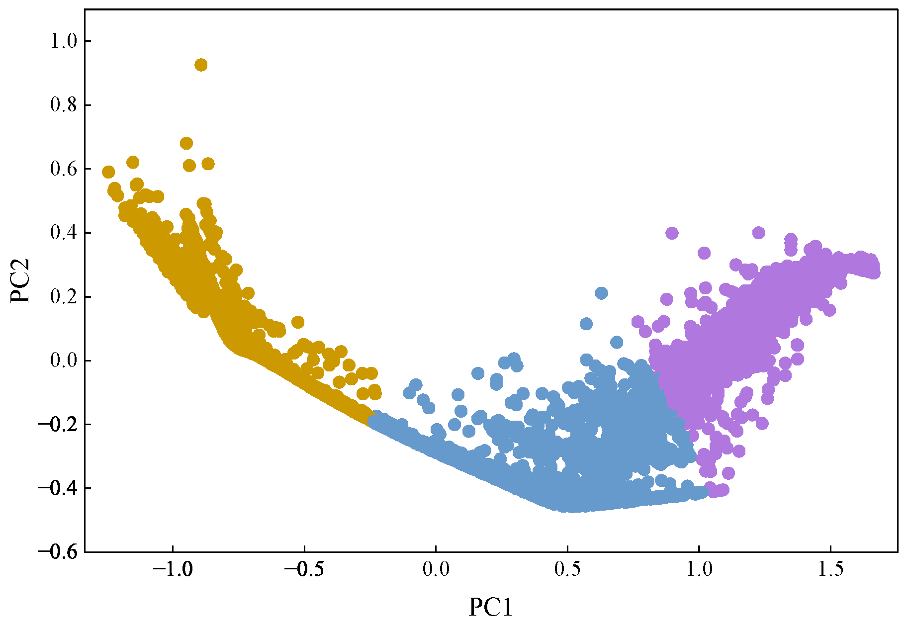
The final operating condition division results are shown in Figure 5. For visualization, the high-dimensional feature data are mapped into a two-dimensional principal component space, where different colors represent different operating condition categories. As shown in Figure 5, the samples can be relatively clearly divided into three cluster regions in the two-dimensional feature space, and different categories generally exhibit good separability. The yellow region on the left corresponds to one type of operating condition, with a relatively concentrated sample distribution, indicating that the turbine operates relatively stably under this condition. The blue region in the middle covers a larger range and shows a certain transitional relationship with the other two operating conditions, suggesting that this condition may correspond to an intermediate operating state with more frequent variations in wind speed and power. The purple region on the right also exhibits good clustering characteristics, indicating that this condition differs relatively clearly from the other two conditions in terms of operating characteristics. Overall, the three operating conditions form a relatively natural distribution structure in the feature space, demonstrating the rationality of using meteorological variables for the operating condition division of wind turbine operational data.

Considering that the occurrence frequencies of different meteorological conditions in actual wind farms are often imbalanced, this paper further counts the number and proportion of samples in the training, validation, and test sets for the three operating conditions, as shown in

Table 6. Sample distribution of the three operating conditions.

Dataset	Condition 1 Samples	Condition 1 Proportion/%	Condition 2 Samples	Condition 2 Proportion/%	Condition 3 Samples	Condition 3 Proportion/%
Training set	2628	35.81	3185	43.40	1526	20.79
Validation set	870	35.57	1056	43.17	520	21.26
Test set	879	35.92	1047	42.79	521	21.29
Total	4377	35.78	5288	43.23	2567	20.99

. These statistics are used to determine whether obvious sample imbalance exists, and to provide a basis for subsequent multi-task loss weight setting and condition-specific forecasting performance analysis.

As shown in Table 6, there are certain differences in the number of samples among the three operating conditions. Condition 2 accounts for the highest proportion, whereas Condition 3 has a relatively lower proportion. This is consistent with the uneven distribution of meteorological conditions in actual wind farms. To reduce the influence of sample size differences on the training process of multi-task learning, the CNTE-MTL model averages the loss within each operating condition task and balances the contribution of different tasks to the overall loss through condition-specific weights. Meanwhile, condition-specific forecasting performance is further reported in the subsequent experiments to examine whether the model performs well only under majority conditions while its performance degrades under minority conditions.

To further verify the applicability of the K-means-based operating condition division method, this paper also compares K-means, Gaussian Mixture Model (GMM), Density-Based Spatial Clustering of Applications with Noise (DBSCAN), and Fuzzy C-Means (FCM) on the same dataset, as shown in

Table 7. Comparison results of different clustering methods.

Clustering     Method	Number of   Conditions	Silhouette   Coefficient	Davies–Bouldin Index	Subsequent Forecasting RMSE
K-means	3	0.6236	0.5088	0.0165
GMM	3	0.6074	0.5312	0.0171
DBSCAN	3	0.5841	0.5749	0.0183
FCM	3	0.6169	0.5226	0.0169

. By comparing clustering metrics, sample distribution, and subsequent forecasting performance among different methods, the influence of the operating condition division method on the forecasting results of CNTE-MTL can be evaluated more comprehensively.

As shown in Table 7, K-means performs better in terms of the Silhouette coefficient, Davies–Bouldin index, and subsequent forecasting RMSE. GMM can characterize certain probabilistic distribution features, but its clustering results are sensitive to distribution assumptions and covariance forms. DBSCAN does not require the number of clusters to be predefined; however, when the density variation of wind power SCADA data is obvious, it is sensitive to the neighborhood radius and the minimum number of samples, and it may easily produce noise points or imbalanced clusters. FCM can provide the membership degree of each sample to different operating conditions, but the subsequent multi-task learning framework in this paper requires explicit task labels for sample routing; therefore, soft labels still need to be converted into hard labels. Considering clustering quality, sample distribution, model implementation complexity, and forecasting performance, this paper finally selects K-means as the meteorology-driven operating condition division method.

It should be noted that, in real-time forecasting scenarios, if meteorological conditions are located near the boundary between two operating conditions and fluctuate frequently, hard condition labels may cause samples to switch frequently between adjacent conditions. In the basic experiments of this paper, the K-means cluster centers determined during the training stage are used for condition assignment; that is, validation and test samples are assigned to operating condition categories according to the distances between their meteorological features and the training cluster centers. Since CNTE-MTL adopts a shared feature extraction network, different operating conditions are not modeled completely independently, which can alleviate prediction discontinuities caused by condition switching to some extent. For practical online deployment, distance-weighted fusion, soft condition membership, or a condition-switching hysteresis mechanism could be further introduced in future work to reduce abrupt prediction changes that may be caused by frequent switching of boundary samples.

3.3. Model Parameters and Evaluation Metrics

Wind power forecasting models usually contain a large number of adjustable parameters, and their performance largely depends on the rationality of parameter configuration. To ensure the objectivity and fairness of the experimental results, this paper adopts the grid search method to systematically optimize the key hyperparameters of each model. The optimal parameter combination is searched within a predefined parameter space, so that the best forecasting performance of each model can be obtained.

To verify the effectiveness of the proposed CNTE-MTL model, three types of comparative experiments are designed in this paper: The first type consists of standard benchmark models, including LSTM, TCN, Transformer, Informer, CNTE, XGBoost, LightGBM, N-BEATS, PatchTST, Autoformer, and FEDformer. These models are trained in a conventional single-task forecasting manner without using operating condition labels; they are mainly used to compare the performance improvement of the proposed method over conventional forecasting models under the same input variables, sliding-window length, and data partitioning scheme. The second type consists of condition-aware benchmark models. Under the same three operating condition division results, several representative benchmark models are trained or evaluated by operating condition, so as to analyze their forecasting performance when condition information is also used. The third type consists of ablation models, including the single-task CNTE without operating condition division, condition-specific independent models using operating condition division but without parameter sharing, and the complete CNTE-MTL model. These models are used to further analyze the contributions of operating condition division, the multi-task sharing mechanism, and condition-specific prediction heads to forecasting performance.

To ensure experimental fairness, all models adopt the same data preprocessing procedure, input variables, training/validation/test set division, sliding-window length, and evaluation metrics. The training, validation, and test sets are divided chronologically at a ratio of 3:1:1. During model training, the Adam optimization algorithm is used to update the parameters of the deep learning models. For machine learning models such as XGBoost and LightGBM, key parameters including tree depth, learning rate, and the number of estimators are determined through grid search. Training is stopped when the validation error does not decrease for 10 consecutive iterations, in order to avoid overfitting. The main hyperparameter settings of each model are shown in

Table 8. Hyperparameter settings of different models.

Model	Hyperparameter Settings
CNTE-MTL	Kernel size = 3; model dimension = 64; number of encoder layers = 2; number of attention heads = 4; feed-forward network dimension = 128; number of operating conditions = 3; sliding-window length = 12; Dropout = 0.1; learning rate = 0.001; batch size = 64; epochs = 100
CNTE	Kernel size = 3; model dimension = 64; number of encoder layers = 2; number of attention heads = 4; feed-forward network dimension = 128; Dropout = 0.1; sliding-window length = 12; learning rate = 0.001; batch size = 64; epochs = 100
Informer	Model dimension = 64; number of encoder layers = 2; number of attention heads = 4; feed-forward network dimension = 128; Dropout = 0.1; sliding-window length = 12; learning rate = 0.001; batch size = 64; epochs = 100
Transformer	Model dimension = 64; number of encoder layers = 2; number of attention heads = 4; feed-forward network dimension = 128; Dropout = 0.1; sliding-window length = 12; learning rate = 0.001; batch size = 64; epochs = 100
TCN	Kernel size = 3; convolution channels = 32 and 64; dilation factors = 1 and 2; number of TCN layers = 2; Dropout = 0.1; fully connected layer dimension = 32; sliding-window length = 12; learning rate = 0.001; batch size = 64; epochs = 100
LSTM	Hidden dimension = 64; number of LSTM layers = 2; Dropout = 0.1; sliding-window length = 12; learning rate = 0.001; batch size = 64; epochs = 100
XGBoost	Number of trees = 300; maximum depth = 5; learning rate = 0.03; subsample = 0.8; colsample_bytree = 0.8; reg_lambda = 1.0
LightGBM	Number of trees = 300; maximum depth = 6; learning rate = 0.03; num_leaves = 31; feature_fraction = 0.8; bagging_fraction = 0.8
N-BEATS	Number of blocks = 3; number of layers per block = 4; hidden units = 128; learning rate = 0.001; batch size = 64; epochs = 100
PatchTST	Patch length = 4; stride = 2; model dimension = 64; number of encoder layers = 2; number of attention heads = 4; Dropout = 0.1; learning rate = 0.001; batch size = 64
Autoformer	Model dimension = 64; number of encoder layers = 2; number of attention heads = 4; decomposition window = 3; feed-forward network dimension = 128; learning rate = 0.001; batch size = 64
FEDformer	Model dimension = 64; number of encoder layers = 2; number of frequency modes = 16; number of attention heads = 4; feed-forward network dimension = 128; learning rate = 0.001; batch size = 64

.

To further verify the role of each component in the proposed model, an ablation study is conducted, as shown in

Table 9. Ablation study settings.

Model	Operating Condition Division	Shared Feature Extraction Network	Condition-Specific Prediction Heads	Experimental Purpose
CNTE	No	–	No	To verify the forecasting performance of the conventional single-task CNTE.
Independent-CNTE	Yes	No	Yes	To verify the effect of independent condition-specific modeling.
CNTE-MTL without task heads	Yes	Yes	No	To verify the effect of a shared model without condition-specific prediction heads.
CNTE-MTL	Yes	Yes	Yes	To verify the effectiveness of the complete multi-task framework.

. Here, CNTE denotes a single-task model without operating condition division or the multi-task mechanism; Independent-CNTE denotes a model that uses the same operating condition division results but trains an independent CNTE model for each condition without sharing feature extraction parameters; CNTE-MTL without task heads denotes a model that uses operating condition division and a shared feature extraction network but does not introduce condition-specific prediction heads; and CNTE-MTL denotes the complete model proposed in this paper, which adopts a shared CNTE feature extraction network and condition-specific prediction heads. Through these comparisons, the contributions of operating condition information, the multi-task sharing mechanism, and condition-specific prediction heads to model performance can be distinguished.

To comprehensively evaluate the forecasting performance of different models, this paper selects the Mean Square Error (MSE), Root Mean Square Error (RMSE), Mean Absolute Error (MAE), and Coefficient of Determination ($R^2$) as evaluation metrics. These metrics reflect model performance from different perspectives, including error magnitude, error stability, and fitting degree; their calculation formulae are as follows:

$$MSE={\displaystyle \frac{1}{N}}{\displaystyle \sum _{i=1}^N}{\left(y_i-{\widehat{y}}_i\right)}^2,$$

(35)

$$RMSE=\sqrt{{\displaystyle \frac{1}{N}}\sum _{i=1}^N{\left(y_i-{\widehat{y}}_i\right)}^2},$$

(36)

$$MAE={\displaystyle \frac{1}{N}}{\displaystyle \sum _{i=1}^N}\left|y_i-{\widehat{y}}_i\right|,$$

(37)

$$R^2=1-{\displaystyle \frac{{\sum }_{i=1}^N{\left(y_i-{\widehat{y}}_i\right)}^2}{{\sum }_{i=1}^N{\left(y_i-\overline{y}\right)}^2}},$$

(38)

where $y_i$ denotes the actual wind power value of the i-th sample, ${\widehat{y}}_i$ denotes the predicted power value, $\overline{y}$ denotes the mean value of the actual power, and N denotes the number of samples. MSE and RMSE are mainly used to measure the overall magnitude of forecasting errors, with RMSE being more sensitive to large errors. MAE reflects the average level of prediction errors and is relatively less sensitive to abnormal errors. $R^2$ is used to evaluate the degree to which the model fits the variation trend of actual power; the closer its value is to 1, the better the forecasting performance.

In addition to the overall test set metrics, this paper further calculates condition-specific forecasting metrics under different meteorological conditions. Since the number of samples under different meteorological conditions in actual wind farms may be imbalanced, reporting only the overall test error may obscure the model’s forecasting performance under minority but critical conditions. Therefore, this paper calculates MSE, RMSE, MAE, and $R^2$ for each operating condition separately, so as to more objectively analyze the adaptability and stability of the model under different meteorology-driven operating states.

To further evaluate the engineering application potential of CNTE-MTL, this paper additionally analyzes the computational complexity, training cost, and scalability of the model. The computational cost of CNTE-MTL mainly comes from the one-dimensional convolutional layer, multi-head self-attention layer, feed-forward network, and condition-specific prediction heads. Let the input window length be L, the input variable dimension be d, the hidden feature dimension be $d_m$, the convolution kernel size be r, the hidden dimension of the feed-forward network be $d_f$, and the number of operating conditions be K. The one-dimensional convolutional layer is mainly used for local temporal feature extraction, and its computational complexity can be approximated as

$$\mathcal{O}\left(Lrd{d}_m\right).$$

(39)

The main computational cost of the multi-head self-attention layer comes from the calculation of the attention matrix, with a complexity of approximately

$$\mathcal{O}\left(L^2{d}_m\right).$$

(40)

Therefore, when the sliding-window length L increases, the self-attention module becomes the component that has the most significant impact on the computational cost of CNTE-MTL. The feed-forward network is used to enhance nonlinear representation capability, and its computational complexity is approximately

$$\mathcal{O}\left(L{d}_m{d}_f\right).$$

(41)

The computational cost of the condition-specific prediction heads is mainly related to the number of operating conditions K and the hidden feature dimension $d_m$. Since this paper adopts a structure consisting of a shared CNTE feature extractor and condition-specific prediction heads, rather than training a complete forecasting model independently for each operating condition, the increase in model parameters and computational cost as K increases is mainly concentrated in the prediction heads, while the shared feature extraction network is not repeatedly expanded. Compared with independent condition-specific modeling, CNTE-MTL can reduce repeated training of the shared feature extraction component, thereby lowering the overall training cost while retaining the ability to model condition-specific differences.

In addition to theoretical complexity analysis, this paper also reports the number of parameters, training time, and average inference time of each model. The number of parameters reflects the model scale, training time measures the offline training cost, and average inference time evaluates the online forecasting efficiency. All models are compared under the same hardware environment, training set division, sliding-window length, and number of training epochs, so as to more intuitively evaluate the trade-off between forecasting performance improvement and computational cost.

3.4. Experimental Results and Analysis

To systematically evaluate the wind power forecasting performance of the proposed CNTE-MTL model at different time scales, comparative experiments were conducted based on actual operational data recorded by the SCADA system of a wind farm. The experimental data cover a continuous 90-day period from January 2024 to March 2024. Considering that the data distribution characteristics and modeling difficulty may differ under different forecasting time spans, we selected a one-month data segment to construct the short-term forecasting experiment, and we selected continuous three-month data to construct a three-month long-term forecasting experiment. These experiments were designed to comprehensively examine the forecasting capability and adaptability of each model under different time-scale scenarios.

In the comparative experiments of this section, CNTE, Informer, Transformer, Temporal Convolutional Network (TCN), and Long Short-Term Memory (LSTM) were selected as the main benchmark models and compared with the proposed CNTE-MTL model. Among them, CNTE was used to verify the forecasting performance of a single shared feature extraction model without the multi-task learning mechanism; Informer and Transformer were used to compare the performance of typical attention-based models in wind power forecasting; and TCN and LSTM represented convolutional temporal models and recurrent neural network models, respectively. To ensure experimental fairness, all models adopted the same data preprocessing procedure, input variables, sliding-window length, and training/validation/test set division method. It should be noted that, except for the proposed CNTE-MTL model, the other benchmark models in this section are trained in a conventional single-task forecasting manner and do not use meteorological condition labels for task routing.

In addition, to further evaluate the engineering applicability of the models, this paper supplements prediction accuracy metrics, including MSE, RMSE, MAE, and $R^2$, with the average inference time of each model. The average inference time represents the average time required for a model to complete one prediction for a single test sample, reflecting the efficiency of online forecasting deployment. It should be noted that the inference time reported in the table is the average inference time per sample, rather than the total inference time for the entire test set. Since the one-month short-term forecasting experiment and the three-month long-term forecasting experiment used the same model structure, input variable dimension, sliding-window length, and hardware environment, the average inference time per sample of the same model remains generally consistent across experiments with different time spans. As the number of test samples increases, the total inference time increases accordingly, but the average inference time per sample is mainly determined by the model structure and input dimension. Figure 6 and Figure 7 show the validation loss curves of different models in the one-month short-term forecasting experiment and the three-month long-term forecasting experiment, respectively.

As shown in Figure 6, in the one-month short-term forecasting task, the validation loss of each model gradually decreases during training, but clear differences exist in convergence speed and stability. Compared with the other benchmark models, the proposed CNTE-MTL model converges more rapidly to a lower loss level and exhibits smaller fluctuations in the later training stage, demonstrating better training stability. The CNTE and Transformer models also show a certain convergence capability, but their overall loss levels and stability are slightly inferior to those of the proposed model. In contrast, the Informer, TCN, and LSTM models exhibit varying degrees of fluctuation or relatively high convergence losses during training, indicating their relatively limited fitting performance in the short-term wind power forecasting task.

As shown in Figure 7, in the three-month long-term forecasting task, the performance differences among different models become more pronounced. Overall, the proposed model still maintains a faster convergence speed and lower validation loss, showing good adaptability for long-term forecasting. By comparison, the other benchmark models generally suffer from larger loss fluctuations or higher convergence levels in the long-term forecasting task, indicating that as the time span increases, it becomes more difficult for the models to characterize complex operating condition variations and long-term temporal features. Taken together, the proposed method exhibits a superior validation performance in both short-term and long-term forecasting tasks, providing a basis for the subsequent comparative analysis of forecasting results.

To further quantify the forecasting performance of different models, this paper comprehensively evaluates the test set prediction results using MSE, RMSE, MAE, $R^2$, and average inference time.

Table 10. Performance evaluation results of different models in the one-month short-term forecasting experiment.

Model	MSE	RMSE	MAE	${\mathit{R}}^2$	Average Inference Time/(ms · Sample−1)
CNTE-MTL	0.0002	0.0165	0.0114	0.9689	0.42
CNTE	0.0003	0.0195	0.0169	0.9565	0.36
Informer	0.0004	0.0211	0.0099	0.9488	0.39
Transformer	0.0005	0.0238	0.0185	0.9352	0.38
TCN	0.0008	0.0285	0.0257	0.9071	0.21
LSTM	0.0011	0.0318	0.0284	0.8841	0.24

and

Table 11. Performance evaluation results of different models in the three-month long-term forecasting experiment.

Model	MSE	RMSE	MAE	${\mathit{R}}^2$	Average Inference Time/(ms · Sample−1)
CNTE-MTL	0.00005	0.0072	0.0052	0.9980	0.42
CNTE	0.0006	0.0246	0.0195	0.9767	0.36
Informer	0.0008	0.0292	0.0242	0.9672	0.39
Transformer	0.0009	0.0302	0.0223	0.9649	0.38
TCN	0.0014	0.0377	0.0302	0.9455	0.21
LSTM	0.0019	0.0443	0.0366	0.9247	0.24

present the performance comparison results of different models in the one-month short-term forecasting experiment and the three-month long-term forecasting experiment, respectively.

As shown in Table 10, in the one-month short-term forecasting experiment, the proposed model achieves the best performance on most evaluation metrics. Specifically, the MSE, RMSE, and $R^2$ of the proposed model reach 0.0002, 0.0165, and 0.9689, respectively, outperforming all comparison models. This indicates that the proposed method has higher forecasting accuracy and better fitting capability in the short-term forecasting task. By comparison, although the performance of the CNTE model is inferior to that of the proposed model, it still outperforms Informer, Transformer, TCN, and LSTM overall. This suggests that introducing a multi-task learning mechanism on the basis of shared feature extraction further enhances the model’s ability to characterize power variation patterns under different operating conditions. The Informer model obtains a relatively small MAE value; however, its MSE, RMSE, and $R^2$ are still inferior to those of the proposed model, indicating that although it achieves smaller average absolute errors on some samples, its overall prediction stability and comprehensive fitting performance still need improvement. Transformer, TCN, and LSTM exhibit relatively larger error metrics—especially TCN and LSTM, whose RMSE and MAE values are noticeably higher. This shows that conventional single-task time-series forecasting models have relatively limited adaptability to the non-stationary characteristics of wind power under complex meteorology-driven conditions.

In terms of average inference time, TCN and LSTM require relatively shorter inference time, indicating that their model structures are comparatively lightweight. CNTE, Transformer, and Informer have slightly higher inference time, mainly due to the attention mechanism and encoder structure. The average inference time of the proposed CNTE-MTL is 0.42 ms/sample, which is higher than that of the ordinary CNTE model but still remains at a low level. The increase in inference time mainly comes from the condition-specific prediction heads and the sample routing process; however, because CNTE-MTL shares the main feature extraction network and does not train a complete independent model for each operating condition, its inference cost remains acceptable for engineering applications.

As shown in Table 11, in the three-month long-term forecasting experiment, the proposed model demonstrates more prominent performance advantages. Specifically, the MSE, RMSE, and MAE of the proposed model are 0.00005, 0.0072, and 0.0052, respectively, while its $R^2$ reaches 0.9980, all of which are significantly better than those of the comparison models. This indicates that the proposed method maintains high forecasting accuracy and good generalization performance over a longer time scale. The three-month dataset covers richer operating states and meteorological variation processes, with a larger sample size and more sufficient operating condition distribution; it can therefore more comprehensively reflect the dynamic evolution patterns of wind power, providing stronger data support for model training and enabling the model to achieve better overall fitting capability in long-term data modeling scenarios.

Further comparison shows that, compared with the short-term forecasting results, the errors of CNTE, Informer, Transformer, TCN, and LSTM increase to varying degrees in the long-term forecasting task, whereas the proposed model still maintains a low error level. This indicates that the meteorology-driven operating condition division mechanism and multi-task collaborative modeling strategy can effectively alleviate the adverse effects caused by operating condition evolution and data distribution changes over a longer time span. Among the comparison models, CNTE still shows certain competitiveness in long-term forecasting, but its MSE, RMSE, and MAE remain clearly inferior to those of the proposed model. This further demonstrates that the multi-task learning strategy has stronger feature sharing and differentiated modeling capabilities under complex operating conditions, thereby helping to improve long-term forecasting performance. In contrast, TCN and LSTM produce the highest errors and relatively lower $R^2$ values in the long-term forecasting task, indicating that these models still have certain limitations in modeling long-term dependencies and characterizing complex operating condition transitions.

Overall, Table 10 and Table 11 show that the proposed model achieves the best results in both short-term and long-term forecasting experiments, with a particularly prominent advantage in the long-term forecasting task. Although the average inference time of CNTE-MTL is slightly higher than that of TCN, LSTM, and ordinary CNTE, its improvement in forecasting accuracy and fitting capability is more significant, indicating that the proposed method achieves a good trade-off between prediction performance and computational cost. These results demonstrate that the proposed method can not only improve wind power forecasting accuracy but also enhance model stability and adaptability under different time scales and complex meteorological conditions.

To more intuitively compare the forecasting performance of different models at different time scales, this paper presents the actual values, model predictions, and corresponding residual variations of the test set in the same figure, so as to comprehensively illustrate the models’ ability to track wind power variation trends and characterize prediction error distributions. Specifically, Figure 8 shows the short-term forecasting results based on one-month data, while Figure 9 shows the long-term forecasting results based on three-month data.

As further shown in Figure 8 and Figure 9, different models exhibit noticeable differences in their ability to track actual values and in the distribution characteristics of residuals. Overall, the proposed model can closely fit the actual variation trajectory of wind power in both short-term and long-term forecasting scenarios; it not only shows a strong ability to track the overall variation trend but also maintains high consistency in intervals with frequent local fluctuations or obvious power abrupt changes. Compared with the other benchmark models, the residual curve of the proposed model is generally closer to the zero axis and exhibits a relatively smaller fluctuation range, indicating that the deviation between the predicted and actual values is smaller and that the error distribution is more concentrated.

Specifically, in the one-month short-term forecasting scenario shown in Figure 8, all models can characterize the overall power variation trend to some extent, but their responses to local peaks, valleys, and rapidly fluctuating intervals differ. The prediction curve of the proposed model shows a high degree of overlap with the actual curve, especially during short-term power fluctuations and staged variation processes, where good synchronization is observed; its residuals are mostly stably distributed around zero, with only slight deviations at a few peak positions. In comparison, the CNTE model performs well overall but still shows certain deviations in some fluctuating intervals. Informer and Transformer respond insufficiently to local variations at some time points, resulting in relatively obvious underestimation or overestimation, and their residual curves also show greater dispersion. Although TCN and LSTM can reflect the basic trend, their ability to characterize complex fluctuation details is relatively limited, leading to persistent deviations between the prediction curves and the actual values in some periods.

From the three-month long-term forecasting results shown in Figure 9, the differences among models become more intuitive as the time span increases and operating condition variations accumulate. The proposed model still maintains good trend-tracking capability over a longer time range and demonstrates strong adaptability around power level changes, stage transitions, and local abnormal fluctuations; this indicates that it can not only learn local temporal features but also effectively capture long-term evolution patterns. Meanwhile, the residual curve of the proposed model remains mainly concentrated near zero, without obvious systematic drift, indicating that it maintains good stability in long-term forecasting. In contrast, the other models generally exhibit varying degrees of error accumulation in the long-term scenario. In particular, after staged changes in power levels, the deviation between the predicted and actual curves becomes more pronounced, and some models show persistently positive or negative residuals, indicating their relatively limited adaptability to long-term operating condition transitions and complex dynamic variations.

In summary, Figure 8 and Figure 9 show that the proposed model has advantages not only in numerical indicators but also in curve-fitting and error stability in the visualization results. Especially when wind power exhibits frequent fluctuations, local abrupt changes, and long-term operating condition evolution, the proposed method can still effectively reduce prediction deviations and keep residuals within a small range. This demonstrates that the model has strong trend characterization and error control capabilities at different time scales, enabling it to adapt more stably to wind power forecasting tasks under complex meteorological conditions. To further reveal the error distribution characteristics of different models in short-term and long-term forecasting tasks, this paper presents boxplots of the residual results of each model, as shown in Figure 10.

As shown in Figure 10, the residual distributions of different models vary between the short-term and long-term forecasting scenarios. Overall, the CNTE-MTL model has narrower residual boxes in both forecasting tasks, with medians closer to the zero axis and relatively shorter upper and lower whiskers; this indicates that its prediction errors are more concentrated, its systematic bias is smaller, and its error stability is better.

In the one-month short-term forecasting scenario, the residuals of all models are generally concentrated; however, CNTE-MTL has the smallest box width and median offset, indicating that it has a stronger ability to track short-term power fluctuations. In comparison, the residual distributions of CNTE, Informer, and Transformer are slightly wider, while TCN and LSTM show greater residual dispersion, suggesting relatively weaker error control capability.

In the three-month long-term forecasting scenario, the residual distributions of the comparison models generally become wider, indicating that as the time span increases, model error fluctuations and the risk of error accumulation increase. In contrast, CNTE-MTL still maintains a smaller residual distribution range and lower median offset, demonstrating that the proposed method retains good prediction stability and generalization capability under long-term operating condition variations. Overall, Figure 10 further verifies the advantages of CNTE-MTL in terms of error concentration and residual stability.

3.5. Supplementary Experimental Analysis

To more comprehensively verify the effectiveness of the proposed CNTE-MTL model, this paper additionally introduces representative models—including XGBoost, LightGBM, N-BEATS, PatchTST, Autoformer, and FEDformer—for experimental comparison. Among them, XGBoost and LightGBM represent traditional ensemble learning models, which can characterize the nonlinear mapping relationship between input variables and output power. N-BEATS is a typical deep time-series forecasting model with strong nonlinear sequence-fitting capability. PatchTST, Autoformer, and FEDformer are Transformer-based models that have commonly been used in long-sequence forecasting tasks in recent years; they enhance time-series feature representation through patch representation, sequence decomposition, and frequency-domain modeling, respectively.

All additional models adopted the same data preprocessing procedure, input variables, sliding-window length, and training/validation/test set division as the proposed model. The newly introduced benchmark models did not use meteorological condition labels and were trained in a standard single-task forecasting manner.

Table 12. Performance evaluation results of additional models in the one-month short-term forecasting experiment.

Model	MSE	RMSE	MAE	${\mathit{R}}^2$	Average Inference Time/(ms · Sample−1)
CNTE-MTL	0.0002	0.0165	0.0114	0.9689	0.42
PatchTST	0.0003	0.0188	0.0137	0.9601	0.45
FEDformer	0.0004	0.0202	0.0151	0.9540	0.54
Autoformer	0.0004	0.0216	0.0160	0.9472	0.51
N-BEATS	0.0005	0.0227	0.0176	0.9405	0.47
LightGBM	0.0006	0.0249	0.0198	0.9286	0.05
XGBoost	0.0006	0.0258	0.0206	0.9224	0.08

and

Table 13. Performance evaluation results of additional models in the three-month long-term forecasting experiment.

Model	MSE	RMSE	MAE	${\mathit{R}}^2$	Average Inference Time/(ms · Sample−1)
CNTE-MTL	0.00005	0.0072	0.0052	0.9980	0.42
PatchTST	0.0004	0.0208	0.0156	0.9832	0.45
FEDformer	0.0005	0.0219	0.0168	0.9819	0.54
Autoformer	0.0005	0.0227	0.0175	0.9804	0.51
N-BEATS	0.0007	0.0264	0.0208	0.9735	0.47
LightGBM	0.0010	0.0321	0.0255	0.9587	0.05
XGBoost	0.0012	0.0342	0.0271	0.9538	0.08

present the performance comparison results between the additional models and CNTE-MTL in the one-month short-term forecasting experiment and the three-month long-term forecasting experiment, respectively.

As shown in Table 12, in the one-month short-term forecasting experiment, long-sequence forecasting models such as PatchTST, FEDformer, and Autoformer generally outperform XGBoost, LightGBM, and N-BEATS. This indicates that deep models based on attention mechanisms, patch-based sequence modeling, and sequence decomposition can more effectively characterize the nonlinear variation patterns in wind power sequences. Among the additional models, PatchTST achieves the best performance, with an RMSE of 0.0188 and an $R^2$ of 0.9601. However, compared with CNTE-MTL, the RMSE of PatchTST is still higher, and its $R^2$ is slightly lower, suggesting that relying solely on patch-based sequence modeling is still insufficient to fully characterize the differences in power evolution patterns under different meteorological conditions.

XGBoost and LightGBM have the shortest inference times, at 0.08 ms/sample and 0.05 ms/sample, respectively, indicating that traditional ensemble learning models have advantages in computational efficiency; however, their prediction errors are clearly higher than those of CNTE-MTL and several deep time-series models. This is mainly because tree-based models are more inclined toward static nonlinear mapping and are insufficient in capturing long-term dependencies within sliding windows, historical dynamic variations, and complex operating condition transition features. Therefore, although these models have low inference costs, their forecasting accuracy remains limited in complex meteorology-driven wind power forecasting scenarios.

As shown in Table 13, in the three-month long-term forecasting experiment, the performance differences among the additional models become more pronounced. PatchTST, FEDformer, and Autoformer still demonstrate strong long-term forecasting capability, indicating that long-sequence forecasting architectures have certain advantages over longer time spans. However, these models mainly improve time-series representation from the perspectives of sequence representation, trend decomposition, or frequency-domain modeling; they do not explicitly use meteorological condition division information, nor do they establish differentiated prediction structures for different operating conditions. Therefore, in long-term forecasting tasks with more complex operating condition evolution, their performance remains clearly inferior to that of the proposed CNTE-MTL model.

In contrast, CNTE-MTL achieves the best results in the three-month long-term forecasting experiment, with an RMSE of only 0.0072 and an $R^2$ of 0.9980. This demonstrates that the proposed method can not only extract common cross-condition temporal features through the shared CNTE network but also characterize differentiated power variation patterns under different meteorological conditions through condition-specific prediction heads, thereby maintaining higher accuracy and stronger stability in long-term forecasting tasks. Although the inference time of CNTE-MTL is higher than those of XGBoost and LightGBM, it remains comparable to or even slightly lower than those of deep long-sequence models such as PatchTST, Autoformer, and FEDformer, while achieving clearly superior forecasting performance. This indicates that the proposed method offers a favorable overall trade-off between forecasting accuracy and computational cost.

Overall, Table 12 and Table 13 further verify the effectiveness of the proposed method through the introduction of additional benchmark models. Compared with traditional ensemble learning models, CNTE-MTL has stronger temporal dependency modeling capability. Compared with typical deep time-series models and Transformer-based long-sequence forecasting models, the advantages of CNTE-MTL mainly arise from meteorology-driven operating condition division and the multi-task collaborative modeling mechanism. This mechanism enables the model to share common information across different operating conditions while preserving condition-specific evolution patterns, thereby improving the accuracy, stability, and adaptability of wind power forecasting under complex meteorological conditions.

3.6. Ablation Study Analysis

To further verify the effectiveness of each component in the CNTE-MTL model, ablation experiments were conducted to analyze the effects of meteorology-driven operating condition division, the multi-task sharing mechanism, and condition-specific prediction heads on forecasting performance. The ablation study included the following four model structures:

(1)

CNTE: Operating condition division and the multi-task mechanism are not used, and all samples are fed into a single CNTE model as one prediction task;

(2)

Independent-CNTE: The same K-means-based operating condition division results are used, but an independent CNTE model is trained separately for each operating condition, without parameter sharing among different conditions;

(3)

CNTE-MTL without Task Heads: Operating condition division and a shared CNTE feature extraction network are used, but condition-specific prediction heads are not introduced, and all operating conditions share the same prediction head;

(4)

CNTE-MTL: The complete model proposed in this paper, which adopts a multi-task structure consisting of a shared CNTE feature extraction network and condition-specific prediction heads.

Through the above ablation settings, the effects of operating condition division, cross-condition parameter sharing, and condition-specific prediction heads on the forecasting results can be examined separately.

Table 14. Performance evaluation results of different ablation models in the one-month short-term forecasting experiment.

Model	MSE	RMSE	MAE	${\mathit{R}}^2$	Average Inference Time/(ms · Sample−1)
CNTE	0.0003	0.0195	0.0169	0.9565	0.36
Independent-CNTE	0.0003	0.0184	0.0148	0.9612	0.37
CNTE-MTL without task heads	0.0003	0.0178	0.0136	0.9640	0.39
CNTE-MTL	0.0002	0.0165	0.0114	0.9689	0.42

and

Table 15. Performance evaluation results of different ablation models in the three-month long-term forecasting experiment.

Model	MSE	RMSE	MAE	${\mathit{R}}^2$	Average Inference Time/(ms · Sample−1)
CNTE	0.0006	0.0246	0.0195	0.9767	0.36
Independent-CNTE	0.0005	0.0218	0.0167	0.9824	0.37
CNTE-MTL without task heads	0.0004	0.0196	0.0142	0.9861	0.39
CNTE-MTL	0.00005	0.0072	0.0052	0.9980	0.42

present the performance comparison results of different ablation models in the one-month short-term forecasting experiment and the three-month long-term forecasting experiment, respectively.

As shown in Table 14, in the one-month short-term forecasting task, clear performance differences can be observed among the ablation models. Compared with the CNTE model without operating condition division, Independent-CNTE reduces the RMSE from 0.0195 to 0.0184 and improves $R^2$ from 0.9565 to 0.9612. This indicates that dividing samples according to meteorology-driven operating conditions can, to some extent, reduce the modeling difficulty caused by the mixture of different operating patterns, thereby improving the forecasting performance. However, Independent-CNTE trains an independent model for each operating condition, without parameter sharing among different conditions; this may lead to insufficient utilization of samples from minority conditions and cannot fully exploit common temporal patterns across different conditions.

In contrast, CNTE-MTL without task heads adopts a shared CNTE feature extraction network and further outperforms Independent-CNTE in terms of RMSE and $R^2$, indicating that cross-condition shared feature extraction helps improve the overall generalization capability of the model. The complete CNTE-MTL model achieves the best results in the short-term forecasting experiment, reducing RMSE to 0.0165 and MAE to 0.0114, while increasing $R^2$ to 0.9689. This suggests that operating condition division alone or shared feature extraction alone is still insufficient to fully characterize the differences in power evolution under different meteorological conditions. Introducing condition-specific prediction heads on the basis of the shared feature extraction network can further enhance the model’s ability to represent condition-specific patterns, thereby achieving higher forecasting accuracy.

As shown in Table 15, the differences among the ablation models become more pronounced in the three-month long-term forecasting experiment. Since the CNTE model does not explicitly consider meteorological condition differences, it produces relatively large prediction errors over the long time span. Independent-CNTE improves upon CNTE, indicating that condition-specific modeling can alleviate the influence of mixed meteorological patterns. However, because the models for different conditions are independent, they cannot share common cross-condition information. When some operating conditions contain relatively fewer samples, insufficient training may occur.

CNTE-MTL without task heads further improves long-term forecasting performance by learning common cross-condition patterns through the shared feature extraction network, demonstrating that the sharing mechanism helps enhance the model’s adaptability to complex long-term data distributions. However, this model does not include condition-specific prediction heads, and all operating conditions share the same output mapping, making it difficult to fully express the differences in power variation patterns under different conditions. The complete CNTE-MTL model integrates both shared feature extraction and condition-specific prediction capability, achieving the best performance in long-term forecasting, with an RMSE of only 0.0072 and an $R^2$ of 0.9980, significantly outperforming the other ablation models.

In terms of inference time, the complete CNTE-MTL model has a slightly higher average inference time than the other ablation models because it introduces condition routing and condition-specific prediction heads. However, the increase is small and remains at the millisecond level, indicating that the multi-task structure does not impose an excessive online forecasting burden. Considering the improvement in forecasting accuracy and stability, the additional inference cost of CNTE-MTL is acceptable.

Overall, the ablation results show that meteorology-driven operating condition division can reduce the modeling difficulty of mixed-condition data; the shared CNTE feature extraction network can promote common information sharing among different conditions; and condition-specific prediction heads can further characterize differentiated power evolution patterns under various meteorological conditions. The synergistic effect of these three components enables CNTE-MTL to achieve higher forecasting accuracy, better error stability, and stronger engineering application potential in both short-term and long-term wind power forecasting tasks.

4. Conclusions

To address the problems of strong non-stationarity in wind power sequences under meteorology-driven operating condition variations, significant differences in power evolution patterns under different operating modes, and insufficient cross-condition forecasting stability of single prediction models, this paper proposes a wind power forecasting method based on the Convolutional Normalized Transformer Encoder and Multi-Task Learning (CNTE-MTL). The proposed method first divides wind turbine operating samples into different conditions according to typical meteorological variables, such as wind speed, wind direction, and ambient temperature, so as to characterize the operating mode differences induced by meteorological variations. On this basis, wind power forecasting under different meteorological conditions is formulated as multiple related subtasks, and a multi-task learning framework consisting of a shared feature extraction network and condition-specific prediction heads is constructed. Short-term forecasting, long-term forecasting, supplementary comparative experiments, and ablation experiments were conducted using SCADA data from an actual wind farm; the main conclusions are as follows:

(1)

Meteorology-driven operating condition division can effectively characterize the differences in wind turbine operating states under different meteorological conditions, providing a reasonable data organization basis for multi-condition wind power forecasting. The experimental results show that when wind speed, wind direction, and ambient temperature are used as condition division variables, the Silhouette coefficient reaches 0.623634 and the Davies–Bouldin index is 0.508835 when the number of clusters is three, indicating that different meteorology-driven operating conditions exhibit good intra-cluster compactness and inter-cluster separability in the feature space. By dividing non-stationary power sequences under complex mixed conditions into representative typical operating conditions, the complexity caused by mixed-mode modeling can be reduced, thereby providing a clearer task structure for the subsequent multi-task forecasting model.

(2)

The constructed CNTE shared feature extraction network can simultaneously extract local temporal fluctuation information and long-term dependency features, helping to improve the representation capability of wind power sequences under complex meteorological disturbances. By introducing a one-dimensional convolutional structure before the Transformer encoder, the model enhances its ability to capture short-term fluctuations, local abrupt changes, and local variation patterns. Meanwhile, with the multi-head self-attention mechanism, the model can further capture dependencies among different time steps within the sliding window. The experimental results show that the CNTE structure achieves a better forecasting performance than traditional temporal models such as TCN and LSTM. After further introducing the multi-task learning mechanism based on CNTE, CNTE-MTL achieves an RMSE of 0.0165 and an $R^2$ of 0.9689 in the one-month short-term forecasting experiment, demonstrating good short-term forecasting accuracy and fitting capability.

(3)

The multi-task learning framework based on a shared feature extraction network and condition-specific prediction heads can effectively improve the model’s generalization capability and forecasting stability under different meteorological conditions. Compared with conventional single-task modeling methods, CNTE-MTL can learn common temporal features across different conditions through the shared network, while characterizing differentiated power evolution patterns under each condition through condition-specific prediction heads. The comparative experimental results show that CNTE-MTL achieves the best forecasting results in both the one-month short-term forecasting task and the three-month long-term forecasting task. In the three-month long-term forecasting experiment, its RMSE is 0.0072, MAE is 0.0052, and $R^2$ reaches 0.9980, significantly outperforming CNTE, Informer, Transformer, TCN, and LSTM, as well as the additionally introduced XGBoost, LightGBM, N-BEATS, PatchTST, Autoformer, and FEDformer models. The ablation experiments further demonstrate that meteorology-driven operating condition division, cross-condition shared feature extraction, and condition-specific prediction heads all contribute positively to model performance improvement, and their synergy can effectively enhance the forecasting adaptability of the model under complex meteorological condition variations.

It should be noted that this study still has certain limitations. First, the experimental data were obtained from a single 1.5 MW direct-drive wind turbine from one wind farm, and the data period mainly covers January to March 2024. The dataset does not yet include year-round multi-seasonal operating data or extreme weather samples such as high temperatures, typhoons, and severe convection. Therefore, the generalization capability of the model across different regions, turbine capacities, and year-round complex meteorological conditions still requires further validation. Second, this study mainly conducted point forecasting based on SCADA data, without modeling forecasting uncertainty; thus, prediction intervals or risk probabilities cannot be directly provided. Third, this paper uses K-means clustering to obtain meteorological condition labels. Although this method is simple to implement and has good interpretability, hard-label switching may still occur near condition boundaries, and further improvements are needed in boundary-sample smoothing and online condition updating mechanisms.

Future research will be carried out in the following directions: First, data sources will be further expanded to include multiple wind farms, turbine types, capacities, and year-round multi-seasonal operating data, so as to verify the generalization capability of the model, with particular attention to forecasting stability under extreme meteorological conditions. Second, numerical weather prediction, air density, pitch angle, yaw error, turbine load, vibration signals, converter states, and other multi-source information will be integrated to enhance the model’s ability to characterize the complete process of “meteorological driving factors, turbine response, and power output”. Third, probabilistic forecasting, interval forecasting, and uncertainty quantification methods will be introduced to provide more reliable confidence ranges for wind power forecasting results. Fourth, soft operating condition division, distance-weighted routing, gating mechanisms, and online learning strategies will be further investigated to improve model robustness under condition-boundary switching and data distribution drift. Fifth, lightweight attention structures, model compression, and incremental updating strategies will be combined to reduce online deployment costs and improve the applicability of the proposed method in actual wind farm operating environments.

References

1. Lu, H.; Gao, X.; Yu, J.; Zhao, Q.; Zhu, X.; Ma, W.; Cao, J.; Wang, Y. Analysis and prediction of incoming wind speed for turbines in complex wind farm: Accounting for meteorological factors and spatiotemporal characteristics of wind farm. Appl. Energy 2025, 381, 125135. [Google Scholar]
2. Mei, Y.; Che, J.; Sun, Q.; Dong, W. An overview of short-term wind power forecasting: Multi-scale decomposition and multi-model deep learning fusion. Energy Strategy Rev. 2026, 63, 102021. [Google Scholar]
3. Li, T.; Ai, L.; Yang, Q.; Zhang, X.; Li, H.; Lu, D.; Shen, H. Short-term wind power prediction based on multiscale numerical simulation coupled with deep learning. Renew. Energy 2025, 246, 122951. [Google Scholar] [CrossRef]
4. Qu, Z.; Hou, X.; Huang, S.; Li, D.; He, Y.; Meng, Y. Probabilistic power forecasting for wind farm clusters using Moran-Graph network with posterior feedback attention mechanism. Energy 2025, 328, 136558. [Google Scholar] [CrossRef]
5. Wang, Q.; Xu, F.; He, J.; Luo, K.; Fan, J. A new fusion model for enhanced ultra-short-term offshore wind power forecasting. Renew. Energy 2026, 256, 123876. [Google Scholar]
6. Wang, W.; Yang, J.; Li, Y.; Ren, G.; Li, K. Data-driven deep learning model for short-term wind power prediction assisted with WGAN-GP data preprocessing. Expert Syst. Appl. 2025, 275, 127068. [Google Scholar]
7. Mustaffa, Z.; Sulaiman, M.H. Random forest based wind power prediction method for sustainable energy system. Clean. Energy Syst. 2025, 12, 100210. [Google Scholar] [CrossRef]
8. Ren, D.; Ma, J.; Liu, H.; Li, Y.; Chen, C.; Qin, T.; He, Z.; Wu, Q. The IVMD-CNN-GRU-attention model for wind power prediction with sample entropy fusion. IEEE Access 2024, 12, 169988–170000. [Google Scholar]
9. Yuzgec, U.; Dokur, E.; Balci, M. A novel hybrid model based on empirical mode decomposition and echo state network for wind power forecasting. Energy 2024, 300, 131546. [Google Scholar] [CrossRef]
10. Melalkia, L.; Berrezzek, F.; Saim, A.; Nebili, R. A hybrid error correction method based on EEMD and ConvLSTM for offshore wind power forecasting. Ocean Eng. 2025, 325, 120773. [Google Scholar] [CrossRef]
11. Liu, H.; Li, P.; Wang, Q. Short-term prediction of wind power based on BKA-CNN-BiGRU-attention. Electr. Power Syst. Res. 2026, 253, 112543. [Google Scholar]
12. Sun, X.; Han, B.; Song, Y.; Wang, Y.; Hou, E.; Wang, J.; Xu, Y. Short-Term Wind Power Forecasting Based on Dual-Optimized VMD-CNN-BiLSTM. Energies 2026, 19, 2317. [Google Scholar] [CrossRef]
13. Wang, Y.; Gao, J.; Xing, H.; Liu, G.; Qi, Y.; Wang, X.; Yang, F. Ultra-short-term wind power prediction method based on optimized signal decomposition and deep learning. Int. J. Electr. Power Energy Syst. 2025, 173, 111417. [Google Scholar]
14. Xin, Z.; Chi, W.; Zhang, H.; Liu, X.; Zheng, G.; Sun, N.; Hou, C.; Chen, L. Ultra short-term wind power prediction based on an improved temporal convolutional network. Int. J. Green Energy 2025, 22, 2899–2919. [Google Scholar] [CrossRef]
15. Ahmadi, M.; Aly, H.; Khashei, M. Enhancing power grid stability with a hybrid framework for wind power forecasting: Integrating Kalman Filtering, Deep Residual Learning, and Bidirectional LSTM. Energy 2025, 334, 137752. [Google Scholar] [CrossRef]
16. Zhao, C.; Wu, Y.; Pan, J.; Chen, P. A physics-aware dynamic graph and mixture-of-experts framework for wind power forecasting. Int. J. Electr. Power Energy Syst. 2026, 176, 111769. [Google Scholar]
17. Yan, Y.; Zhang, Y.; Jiang, J.; Zhang, P. A spatiotemporal fusion network based on Mamba and GCN for wind power forecasting. J. Renew. Sustain. Energy 2025, 17, 036103. [Google Scholar] [CrossRef]
18. Zhang, X.; Li, T.; Yang, Q.; Zhou, X.; Benini, E. A novel non-dimensional multiple operating conditions physics-informed neural networks for wind turbine wake and power prediction in complex terrains. Energy 2026, 358, 141301. [Google Scholar] [CrossRef]
19. Zhang, C.; Xiao, X.; Wang, Y.; Hou, M.Z.; Huang, S.; Hu, W.; Hu, M.; Huang, R. Fine-grained ultra-short-term wind power forecasting based on Temporal Fusion Transformers integrated with turbine power time series clustering. Energy 2025, 335, 137995. [Google Scholar]
20. Lin, L.; Xu, J.; Liu, J.; Zhang, H.; Gao, P. Short-term wind power forecasting method for extreme cold wave conditions based on small sample segmentation. Int. J. Electr. Power Energy Syst. 2025, 170, 110876. [Google Scholar] [CrossRef]
21. Deng, Z.; Zhang, X.; Li, Z.; Yang, J.; Lv, X.; Wu, Q.; Zhu, B. Probabilistic prediction of wind power based on improved Bayesian neural network. Front. Energy Res. 2024, 11, 1309778. [Google Scholar] [CrossRef]
22. Tian, C.; Niu, T.; Li, T. Developing an interpretable wind power forecasting system using a transformer network and transfer learning. Energy Convers. Manag. 2025, 323, 119155. [Google Scholar]
23. Liu, H.; Zhao, J.; Pan, C.; Mao, L. Data-driven real-time wind power forecasting based on the dynamic adaptive selective state space model (DA-SSSM). Electr. Power Syst. Res. 2026, 250, 112176. [Google Scholar]
24. Liu, L.; Liu, J.; Ye, Y.; Liu, H.; Chen, K.; Li, D.; Dong, X.; Sun, M. Ultra-short-term wind power forecasting based on deep Bayesian model with uncertainty. Renew. Energy 2023, 205, 598–607. [Google Scholar]
25. Isik, M.; Yalcinkaya, M.a. Integrated regime-aware wind power forecasting using multi-altitude meteorological features and hybrid machine learning. Front. Energy Res. 2025, 13, 1686125. [Google Scholar]
26. Chen, J.; Zhang, Z.; Liu, M.; Yan, D.; Tang, X. A novel method for wind power abnormal data identification and cleaning based on boundary modeling. IEEE Trans. Instrum. Meas. 2025, 74, 3543412. [Google Scholar] [CrossRef]
27. Abdel-Wahed, A.T.; Taha, W.A.; Abdel-Moneim, M.G.; Abdel-Khalik, A.S.; Mansouri, M.; Ahmed, S. Real wind data clustering for optimal design of a 12-slot/10-pole PMSG in wind power applications. Ain Shams Eng. J. 2026, 17, 104018. [Google Scholar] [CrossRef]
28. Wang, P.; Wang, L.; Huang, S.; Zhang, J.; Wei, J. A novel Data-Model Hybrid-Driven strategy for voltage control and noise resistance in wind farm. Int. J. Electr. Power Energy Syst. 2026, 176, 111666. [Google Scholar]
29. Xu, P.; Zhang, S.; Luo, P.; Wang, X.; Yan, Y.; Qi, D. Data-feature hybrid optimization for ultra-short-term wind power forecasting. Int. J. Electr. Power Energy Syst. 2026, 176, 111742. [Google Scholar]
Figure 1. Overall framework of multi-task wind power forecasting based on CNTE-MTL.
Energies 19 03111 g001
Figure 2. Schematic diagram of the CNTE encoding block.
Energies 19 03111 g002
Figure 3. Schematic diagram of the 1.5 MW direct-drive wind turbine.
Energies 19 03111 g003
Figure 4. Cleaning of wind power data: (a) before data cleaning; (b) after data cleaning.
Energies 19 03111 g004
Figure 5. Clustering results of typical operating conditions of the wind turbine. Different colors represent different meteorology-driven operating condition categories; specifically, yellow, blue, and purple indicate the three clustered operating conditions.
Energies 19 03111 g005
Figure 6. Validation loss curves of different models in the one-month short-term forecasting experiment.
Energies 19 03111 g006
Figure 7. Validation loss curves of different models in the three-month long-term forecasting experiment.
Energies 19 03111 g007
Figure 8. Forecasting results and residual variations of different models in the one-month short-term forecasting experiment.
Energies 19 03111 g008
Figure 9. Forecasting results and residual variations of different models in the three-month long-term forecasting experiment.
Energies 19 03111 g009
Figure 10. Residual boxplots of different models in short-term and long-term forecasting tasks.
Energies 19 03111 g010