Probabilistic Forecasting of Regional Photovoltaic Power Based on QR-STGAT

Abstract

As the penetration rate of photovoltaic power generation continues to increase within new power systems, accurately forecasting regional PV power output has become critical to ensuring the safe and stable operation of power grids. Photovoltaic power generation exhibits significant spatio-temporal correlations, and traditional single-site forecasting methods struggle to fully capture the spatial dependencies among multiple PV plants within a region. To address this challenge, this study proposes a unified QR-STGAT probabilistic forecasting framework that jointly captures adaptive spatial dependencies via graph attention mechanisms and multi-scale temporal dynamics via a CNN-GRU architecture, while enabling end-to-end uncertainty quantification through integrated quantile regression. The framework is validated on 15 min resolution PV output data collected from five prefecture-level cities in Guangdong Province over a seven-month period from January to July 2025, and compared against baselines including BiLSTM and Transformer. Experimental results demonstrate that the proposed method reduces RMSE by up to 11.61% over baseline models and achieves a PICP of 93.05% at the 95% confidence level, providing a more reliable reference for power system dispatch decisions.

1. Introduction

Against the backdrop of global carbon neutrality goals, photovoltaic (PV) power generation—as a vital component of clean renewable energy—has become a key pillar in building new power systems. According to data released by the International Renewable Energy Agency (IRENA), global PV installed capacity continues to grow rapidly, projected to exceed 5000 GW by 2030 [1]. However, the inherent volatility, intermittency, and uncertainty of PV generation pose severe challenges to the safe and stable operation of power grids [2]. This uncertainty primarily stems from the rapid fluctuations in solar irradiance, which is governed by a complex interplay of factors including cloud movement, aerosol concentration, and atmospheric transmittance. Accurate PV power forecasting can effectively support grid dispatch decisions, optimize unit operation, reduce reserve capacity requirements, and provide reliable assurance for integrating new energy sources [3].

Traditional photovoltaic power forecasting methods primarily include physical methods, statistical methods, and machine learning methods [4]. Physical methods, based on Numerical Weather Prediction (NWP) and radiation transfer models, can provide medium-to-long-term forecasts but involve high computational complexity and sensitivity to initial conditions [5]. Statistical methods, such as Autoregressive Moving Average (ARMA) models and Kalman filters, are suitable for short-term forecasting but struggle to capture nonlinear dynamic characteristics. With advancements in artificial intelligence, machine learning approaches like Support Vector Machines (SVM) and Random Forests (RF) have gained widespread adoption in PV forecasting, demonstrating strong nonlinear fitting capabilities [6].

With the advancement of artificial intelligence technology, deep learning methods such as CNNs, Long Short-Term Memory (LSTM) networks, and GRUs have been widely applied in the field of photovoltaic power forecasting [7,8]. Reference [9] achieved high prediction accuracy by integrating the Transformer and BiLSTM architectures, leveraging the Transformer’s self-attention mechanism to capture global dependencies while combining the bidirectional temporal modeling capabilities of BiLSTM. However, these methods treat each PV plant as an independent node and model only the temporal dynamics of individual sites, with no mechanism to propagate or aggregate information across spatially distributed stations. As a result, inter-station dependencies arising from shared meteorological conditions and cloud movement patterns are entirely disregarded, limiting their applicability in regional forecasting scenarios where spatiotemporal coupling relationships among multiple power plants are of central importance. Fully leveraging these spatiotemporal dependencies is therefore crucial for improving the accuracy of regional photovoltaic power forecasting [10].

In recent years, Graph Neural Networks (GNNs) have provided novel approaches for regional spatio-temporal forecasting due to their advantage in handling non-Euclidean data structures [11]. GNNs model data as graph structures, effectively capturing complex spatial dependency patterns through information propagation and aggregation on the graph. Reference [12] employs sparse spatio-temporal attention to filter weak correlations among photovoltaic (PV) stations, utilizing adaptive adjacency matrices and temporal convolutional networks to capture latent spatio-temporal dependencies among PV sites. Reference [13] employs Spatio-Temporal Graph Convolution Networks (STGCN) for regional load forecasting. It constructs graph topologies to represent spatial relationships between nodes while integrating temporal models to capture time dependencies. However, graph convolutional networks employ fixed weights when aggregating neighboring node information, failing to adaptively learn the importance of different nodes. STGAT dynamically adjusts node weights by introducing an attention mechanism, thereby better capturing complex spatial dependencies [14].

Furthermore, traditional point forecasting methods provide only a single predicted value, making it difficult to quantify power uncertainty. In actual power grid dispatch, decision-makers need not only to know the expected power value but also to understand its potential fluctuation range to formulate reasonable reserve capacity plans and dispatch strategies. Probabilistic forecasting, by constructing confidence intervals, can more comprehensively reflect the range of photovoltaic power fluctuations, providing more reliable decision-making support for grid dispatch [15]. Reference [16] optimizes probabilistic forecasting models to narrow interval widths by obtaining quantiles for upper and lower bounds through adaptive two-layer optimization, while ensuring interval reliability. As a nonparametric method, quantile regression directly estimates conditional quantiles without requiring error distribution assumptions, offering strong robustness and flexibility. Reference [17] applied this to photovoltaic power probabilistic forecasting. By introducing a monotonicity constraint penalty term to ensure reasonable ordering of different quantile forecast values, it enhanced the performance of the prediction interval. Reference [7] employs fuzzy C-means clustering to segment similar days, then combines QR, CNN, and BiLSTM neural networks for fine-grained classification prediction at 5 min intervals, generating reliable forecast intervals. The QR-based probabilistic forecasting algorithm offers high flexibility; when integrated with artificial intelligence methods, it can further construct high-dimensional nonlinear mapping relationships, finding extensive application in probabilistic forecasting of renewable energy output [18].

A review of existing research reveals that despite advances in both deep learning methods and probabilistic forecasting techniques, the following limitations persist: (1) Most studies treat photovoltaic power plants as isolated systems, failing to fully leverage spatial correlations among plants within a region; (2) Current spatiotemporal forecasting models predominantly employ fixed spatial aggregation weights, lacking adaptability to dynamic meteorological conditions; (3) Point forecasts and probability forecasts are often conducted separately, failing to simultaneously achieve high-precision point forecasts and reliable interval estimates within a unified framework. To address these limitations, this paper proposes a unified probabilistic forecasting framework that integrates adaptive spatial topology modeling, spatio-temporal feature extraction, and quantile regression-based uncertainty quantification.

Based on the above analysis, this paper proposes a regional PV power probabilistic forecasting method integrating spatio-temporal graph attention networks and quantile regression. The main contributions of this paper include:

• Proposing a spatio-temporal prediction framework that integrates a graph attention mechanism. By constructing an adaptive graph topology based on the geographical locations and historical power correlations of PV power plants, the Graph Attention Layer (GAT) adaptively learns the spatial weights of nodes at different time points, effectively capturing dynamically changing spatial dependencies.
• A multi-scale temporal representation mechanism is introduced to jointly capture local meteorological fluctuations and long-range temporal dependencies. By leveraging CNN to extract local multi-scale patterns from multidimensional meteorological inputs and GRU to model long-range sequential evolution, the two components play complementary roles within the spatiotemporal framework, enabling richer temporal representations and improving the model’s capacity to track complex photovoltaic power dynamics.
• A unified end-to-end probabilistic forecasting framework is established by integrating quantile regression into the STGAT architecture, eliminating the need for separate point and interval forecasting pipelines. By jointly optimizing multiple quantile loss functions within a shared encoder structure, the framework achieves simultaneous high-precision point prediction and reliable interval estimation, representing a methodologically integrated alternative to conventional two-stage forecasting approaches.
• Case studies using actual PV data from Guangdong Province demonstrate that the proposed method outperforms existing benchmark approaches in both point prediction accuracy metrics (e.g., root mean square error RMSE, mean absolute error MAE) and interval prediction evaluation metrics (e.g., probability of interval coverage PICP, probability of interval average width PINAW), validating its effectiveness and practicality.

The remainder of this paper is organized as follows: Section 2 analyzes the spatiotemporal correlations of regional PV output; Section 3 details the proposed QR-STGAT model; Section 4 presents the overall forecasting framework; Section 5 conducts case studies and comparative experiments; Section 6 summarizes the findings and outlines future research directions.

2. Analysis of Spatiotemporal Correlation Characteristics of Regional Photovoltaic Power

The power output of regional photovoltaic power stations exhibits significant spatiotemporal coupling characteristics. In-depth analysis of its intrinsic spatial correlation structure and dynamic transmission mechanisms is a prerequisite for constructing high-precision regional forecasting models. To quantify the spatial correlation of regional photovoltaic power, this section introduces the concept of adjacency matrices from graph theory to construct spatial topological networks. Based on actual medium-voltage photovoltaic data from five representative cities in Guangdong Province (Dongguan, Foshan, Guangzhou, Jiangmen, and Zhongshan) in 2025, we conduct spatiotemporal correlation analysis of regional photovoltaic power. These cities were selected based on their geographic proximity within the Pearl River Delta region, their strong pairwise power correlations as evidenced by Pearson correlation coefficients ranging from 0.88 to 0.95 (Figure 1), and the availability of complete and continuous data records over the study period. The adjacency matrix $A$ encodes the topological connectivity between nodes, where its elements $a_{ij}$ are defined as:

$$a_{ij}=\left\{\begin{array}{c}1,\begin{array}{cc}& \end{array}\rho \left(i,j\right)\ge \theta \\ 0,\begin{array}{cc}& \end{array}\rho \left(i,j\right)<\theta \end{array}\right.$$

(1)

In the formula, $\rho \left(i,j\right)$ represents the Pearson correlation coefficient between node $i$ and node $j$; $\theta$ denotes the correlation threshold. This section employs the Pearson correlation coefficient to quantify the correlation degree among photovoltaic power sequences across cities, calculated as follows:

$$\rho \left(i,j\right)={\displaystyle \frac{ Cov\left(P_i, P_j\right)}{{\sigma }_i{\sigma }_j}}$$

(2)

In the formula, $Cov\left(\cdot \right)$ denotes the covariance, and $\sigma$ denotes the standard deviation.

Considering the sparsity and computational efficiency of the network, this paper sets a correlation threshold $\theta =0.89$. When $\rho \left(i,j\right) \ge 0.89$, a significant power correlation is deemed to exist between two cities, and the adjacency matrix is assigned a value of 1; otherwise, it is assigned a value of 0. This threshold preserves strong correlations while avoiding the computational burden caused by overly dense network structures.

Figure 1 illustrates the geographical distribution of five representative cities in Guangdong Province and a schematic representation of the adjacency matrix constructed based on power correlation. Boxes and “*” indicate locations where the power correlation coefficient between two cities exceeded the set threshold, suggesting a connection exists between them and they can share time-series information. The left map displays the geographical locations of each city, while the right heatmap quantifies the power correlation coefficients between cities. The figure reveals highly synchronized photovoltaic output across the Pearl River Delta region. The pairwise Pearson correlation coefficients among the five cities range from 0.88 to 0.95, with a mean of 0.904, reflecting consistently strong inter-city power correlations driven by shared meteorological conditions. Under the adopted threshold of $\theta = 0.89$, nine out of ten possible city pairs satisfy the connectivity condition, yielding a graph with an edge density of 90%. This near-complete connectivity confirms the strong spatiotemporal coupling within the region, while the exclusion of the one weakest pair ensures the graph topology remains statistically grounded rather than arbitrarily fully connected.

The above analysis demonstrates that regional PV power exhibits significant spatiotemporal coupling characteristics and strong spatial correlation. Traditional single-site forecasting methods fail to capture the dynamic correlation transmission mechanisms between sites and struggle to quantify the uncertainty boundaries of predictions. Consequently, they no longer meet the dual demands of grid dispatch for precise regional PV power forecasting and risk assessment. Therefore, there is an urgent need to establish an integrated forecasting framework that combines spatial topology modeling, temporal dynamic evolution, and probabilistic interval estimation. Based on this, this paper proposes an integrated regional PV power probabilistic forecasting framework combining Spatio-Temporal Graph Attention Networks (STGAT) with quantile regression, enabling high-precision spatiotemporal feature extraction and uncertainty quantification.

3. Principles of the QR-STGAT Model

3.1. Spatio-Temporal Attention Network

3.1.1. Graph Data Structures

A graph is a non-Euclidean data structure composed of a set of nodes and a set of edges, used to represent relationships between nodes. In photovoltaic power forecasting scenarios, each photovoltaic power plant can be represented as a node in the graph, and the spatial correlation between plants can be characterized by edges. Formally, a graph can be defined as:

$$G=\left(V,E\right)$$

(3)

Here, $V=\left\{v_1, v_2, \dots , v_n\right\}$ denotes the set of N nodes, and $E\subseteq V\times V$ denotes the set of edges. The topological structure of a graph can be represented by an adjacency matrix $A\in {\mathbb{R}}^{N\times N}$, whose elements $A_{ij}$ denote the connection weights between nodes $v_i$ and $v_j$. For photovoltaic power plant networks, the adjacency matrix can be constructed based on geographical location and power-related dependencies.

Considering geospatial distance and power-time sequence similarity, this paper employs a combined approach of Gaussian kernel functions and maximum mutual information coefficients [19] to construct the graph topology matrix. MIC detects both linear and nonlinear dependencies between power sequences without imposing assumptions on the underlying functional form, making it more expressive than Pearson correlation alone for characterising complex inter-station relationships [19].

$$A_{ij}=\left\{\begin{array}{ll}exp\left({\displaystyle \frac{-ED{\left(i,j\right)}^2}{{\sigma }^2}}\right)\cdot MIC\left(i,j\right),& if MIC\left(i,j\right)\ge \theta \\ 0,& otherwise\end{array}\right.$$

(4)

Here, $ED\left(i,j\right)$ denotes the Euclidean distance between power plants $i$ and $j$, $\sigma$ represents the standard deviation of the distance, $MIC\left(i,j\right)$ indicates the maximum mutual information coefficient between the power sequences of the two plants, and $\theta$ is the correlation threshold.

3.1.2. Graph Attention Mechanism

Graph convolutional networks update the feature representation of a central node by aggregating information from neighboring nodes. However, this aggregation process assigns equal weights to all neighbors, ignoring differences in their relative importance. Graph attention networks introduce an attention mechanism that enables adaptive learning of the contribution levels from different neighbors to the central node [20].

The following notation is used consistently in Equations (5)–(13), as summarised in

Table 1. Notation used in Equations (5)–(13).

Symbol	Category	Description
$F,F^{\prime }$	Dimension	Input/output feature dimensions of GAT.
$X\in {\mathbb{R}}^{N\times T\times D}$	Tensor	Input spatiotemporal feature tensor.
$h_i,h_j\in {\mathbb{R}}^F$	Vector	Feature vectors of nodes i and j.
$W\in {\mathbb{R}}^{F\times F^{\prime }}$	Matrix	Learnable transformation matrix.
$a\in {\mathbb{R}}^{2F^{\prime }}$	Vector	Attention weight vector.
${\alpha }_{ij}$	Scalar	Normalized attention weight.
$W_c,\hspace{0.33em}{b}_c$	Matrix/Vector	CNN layer weight matrix and bias vector.
$r,\hspace{0.33em}z,\hspace{0.33em}\tilde{h}$	Vector	GRU reset gate, update gate, candidate state.
$\odot$	Operator	Element-wise multiplication.
$\sigma (\cdot )$	Operator	Nonlinear activation function

.

As shown in Figure 2, for node $i$, its set of neighboring nodes is denoted as $N_i$. The attention scores between node $i$ and its neighboring nodes $j$ are computed via the attention function as follows:

$$e_{ij}=a([W{h}_i,W{h}_j])$$

(5)

Here, $h_i\in {\mathbb{R}}^F$ and $h_j\in {\mathbb{R}}^F$ denote the input feature vectors of nodes i and j, respectively, where F is the input feature dimension. $W\in {\mathbb{R}}^{F^{\prime }\times F}$ is a learnable linear transformation matrix, where F′ is the output feature dimension, and $a\left(·\right)$ is the attention function. $h_i^{\prime }\in {\mathbb{R}}^{F^{\prime }}$ denotes the updated feature vector of node i.

This paper implements the attention function using a single-layer feedforward neural network with LeakyReLU as the activation function. The attention scores are normalized to obtain the attention weights:

$${\alpha }_{ij}={\mathrm{softmax}}_j(e_{ij})={\displaystyle \frac{\exp (\mathrm{LeakyReLU}(e_{ij}))}{{\displaystyle \sum _{k=1}^N\exp }(\mathrm{LeakyReLU}(e_{ik}))}}$$

(6)

By performing a weighted summation of neighbor node features based on attention weights, node features can be updated as follows:

$$h_{i^{\prime }}=\sigma \left({\alpha }_{ii}W{h}_i+{\displaystyle \sum _{j\in N_i}{\alpha }_{ij}}W{h}_j\right)$$

(7)

Here, $\sigma \left(·\right)$ denotes the nonlinear activation function, and $h_i^{\prime }$ represents the updated feature representation of the node $i$. Through this approach, GAT can adaptively learn the spatial correlation strengths between different photovoltaic power plants, providing more precise spatial feature representations for the prediction model.

3.1.3. Spatio-Temporal Attention Network Architecture

The Spatio-Temporal Graph Attention Network integrates graph attention networks with recurrent neural networks to model spatio-temporal data. The overall architecture adopts a feature fusion strategy: at each time step, GAT extracts spatial features, CNN extracts multidimensional features, and GRU captures temporal dependencies.

As shown in Figure 3, for the regional photovoltaic power forecasting problem, the input data is represented as $X\in {\mathbb{R}}^{N\times T\times F}$, where $N$ denotes the number of photovoltaic power plants, $T$ represents the historical time step, and $F$ indicates the feature dimension. For the forecasting objective of predicting power values over the next p time steps, the computational workflow of the STGAT model is as follows:

• Graph Attention Layer: For the input at time step, spatial features are extracted via GAT:

$$H_t^{(1)}=GAT\left(X_t, \tilde{A}\right)$$

(8)

Here, $\tilde{A}=A+I$ denotes the adjacency matrix containing self-loops, and $I$ denotes the identity matrix.

2.

Convolution Layer: Extracts the interaction relationships among multidimensional features through a 1D-CNN network:

$$H_t^{(2)}=f\left(W_c\ast H_t^{(1)}+b_c\right)$$

(9)

Here, $\ast$ denotes the convolution operation, $W_c$ and $b_c$ are the parameters of the convolution layer, and $f(\cdot )$ is the activation function.

3.

Gated Recurrent Unit: Captures temporal dependencies through GRU. The GRU comprises a reset gate and an update gate, with the computation process as follows:

$$r_t=\sigma \left(W_r\left[h_{t-1}, H_t^{(2)}\right]+b_r\right)$$

(10)

$$z_t=\sigma \left(W_z\left[h_{t-1}, H_t^{(2)}\right]+b_z\right)$$

(11)

$${\tilde{h}}_t=tanh(W_h[r_t\odot h_{t-1},H_t^{(2)}]+b_h)$$

(12)

$$h_t=(1-z_t)\odot h_{t-1}+z_t\odot {\tilde{h}}_t$$

(13)

Here, $r_t$ and $z_t$ represent the reset gate and update gate, respectively; ${\tilde{h}}_t$ denotes the candidate state, $h_t$ denotes the final output state, and $\odot$ indicates element-wise multiplication.

4.

Output Layer: Maps hidden states to predicted outputs through a fully connected layer.

$$\widehat{y}=W_o{h}_t+b_o$$

(14)

Among these, $\widehat{y}$ is the predicted output, and $W_o$ and $b_o$ are the parameters of the output layer.

Figure 3. The Overall Architecture of the Spatio-Temporal Graph Attention Network (STGAT), illustrating spatial feature extraction via GAT and CNN, sequential unfolding across T time steps, temporal modeling via GRU, and point prediction via a fully connected layer.

Figure 3. The Overall Architecture of the Spatio-Temporal Graph Attention Network (STGAT), illustrating spatial feature extraction via GAT and CNN, sequential unfolding across T time steps, temporal modeling via GRU, and point prediction via a fully connected layer.

3.2. Quantile Regression

Quantile regression is a statistical method proposed by Koenker and Bassett in 1978 for estimating conditional quantiles rather than conditional means. Unlike traditional least squares regression, quantile regression estimates regression coefficients at different quantile levels by minimizing an asymmetric loss function [21].

As shown in Figure 4, for a given quantile level $\tau \in \left(0,1\right)$, the objective of quantile regression is to find the parameter $\beta$ such that the quantile loss function $\tau$ is minimized:

$${\min }_{\beta }{\displaystyle \frac{1}{n}}{\displaystyle \sum _{i=1}^n{\rho }_{\tau }}\left(y_i-x_i^T\beta \right)$$

(15)

Among these, the quantile loss function ${\rho }_{\tau }(u)$ is defined as:

$${\rho }_{\tau }(u)=u\left(\tau -1\left\{u<0\right\}\right)$$

(16)

Here, $1\left\{\cdot \right\}$ denotes the indicator function. When $u\ge 0$, the loss function is $\tau \left|u\right|$; otherwise, it is $\left(1-\tau \right)\left|u\right|$. This asymmetric loss function imposes different penalties on positive and negative errors, thereby estimating predicted values at different quantile levels. Combining quantile regression with STGAT enables end-to-end probabilistic forecasting. Quantile regression is preferred over alternative approaches such as Bayesian methods for three reasons: it requires no prior assumptions on the error distribution, which is important given the non-Gaussian nature of PV output uncertainty; it integrates naturally into gradient-based deep learning training via the pinball loss without requiring approximate inference or sampling procedures; and it allows simultaneous estimation of multiple quantile levels within a single shared encoder, making it computationally efficient and architecturally consistent with the proposed framework. For different quantile levels $\tau$, independent model parameters ${\theta }_{\tau }$ are trained to minimize the quantile loss function:

$$L\left({\theta }_{\tau }\right) = {\displaystyle \frac{1}{n}}{\displaystyle {\sum }_i{\rho }_{\tau }\left(y_i- f_{{\theta }_{\tau }}\left(x_i\right)\right)}$$

(17)

Among these, $f_{{\theta }_{\tau }}\left(x_i\right)$ denotes the model’s predicted output at the percentile level $\tau$.

4. A QR-STGAT-Based Probabilistic Power Forecasting Model for Regional Photovoltaic Systems

To fully leverage spatial correlation information among regional photovoltaic systems, enhance the accuracy of PV power forecasting, and characterize the uncertainty in PV output, this study employs a spatio-temporal graph attention network to capture spatial dependencies and temporal evolution patterns between PV power plants. Building upon the point prediction outputs, the framework integrates quantile regression to derive probabilistic prediction intervals at varying confidence levels. The specific construction process of the QR-STGAT-based regional PV power probabilistic forecasting model is as follows.

• Preprocess historical output data and irradiance data from photovoltaic power plants within the region. Simultaneously, handle missing and outlier values, and normalize all features to the [0, 1] range using the min–max normalization method.
• Construct the graph topology structure of regional photovoltaic power stations. Calculate power correlations based on historical power sequences from each photovoltaic power station, and use these power correlations to construct the graph topology matrix A reflecting spatial relationships.
• Divide the processed dataset into training and testing sets in an 8:2 ratio based on chronological order. Define the quantile loss function using Equations (15) and (16) and preset multiple quantile points.
• Construct and train the STGAT model. Input historical data and graph topology into the STGAT model. The embedding layer maps raw features to a hidden space, followed by sequential processing through graph attention layers, convolutional layers, and gated recurrent units to extract spatio-temporal dependency features. The training objective is to minimize the total loss function:

$$L={\displaystyle \frac{1}{\left|\tau \right|}}{\displaystyle {\sum }_{\tau }{L}_{\tau }+\lambda \left|\right|\theta |{|}^2}$$

(18)

In the equation, $L_{\tau }={\displaystyle \frac{1}{n}}{\displaystyle {\displaystyle \sum }_{i=1}^n}{\rho }_{\tau }(y_i-f_{{\theta }_{\tau }}(x_i))$ denotes the quantile loss at quantile level $\tau$ as defined in Equations (15) and (16), $\left|\tau \right|$ denotes the total number of quantile levels, and $\lambda \parallel \theta {\parallel }^2$ represents the L₂ regularization term which prevents model overfitting. The total loss L is therefore the average quantile loss across all quantile levels plus the regularization penalty. For different quantile levels $\tau$, the model shares encoder parameters and uses independent parameters only in the output layer.

5.

After model training is complete, input the test set for point forecasting to derive regional photovoltaic output point forecast curves at each preset percentile. Based on the point forecast results, calculate the point forecast error evaluation metrics.

6.

Given a confidence level, combine the aforementioned percentile calculation results to determine the confidence interval at the specified confidence level. Calculate the corresponding probability forecast metrics to complete the solution for the probability forecast interval. For a prediction interval with confidence level $(1-\alpha )$, the upper and lower bounds are determined by the predicted values at quantile levels $U_{\alpha }=1-\alpha /2$ and $L_{\alpha }=\alpha /2$ respectively, where $U_{\alpha }$ and $L_{\alpha }$ denote the upper and lower quantile levels corresponding to the given confidence level.

7.

Conduct comparative experiments using different benchmark methods, organize the prediction results, and evaluate the prediction performance.

The QR-STGAT-based regional PV power probabilistic forecasting framework is illustrated in Figure 5. The overall process is organised into three sequential phases: data preprocessing, STGAT model construction, and predictive output, each of which is described in detail in the caption of Figure 5.

5. Case Study Analysis

5.1. Data Preprocessing

This study is based on actual photovoltaic operational data collected from January to July 2025 across five cities in Guangdong Province, China. Data was sampled at 15 min intervals, encompassing seven months of observation records with a total of 96 data points per day. The dataset includes photovoltaic power output and solar irradiance data collected under Guangdong Province’s subtropical monsoon climate, which is characterised by abundant solar radiation alongside frequent cloud cover variations and high humidity, particularly during the wet season. As the data are aggregated at the city level, individual plant counts and exact installed capacities are not directly available; the peak installed capacity of each city is estimated from the maximum observed power output over the study period, with the five cities collectively representing a substantial share of the medium-voltage PV installations in the Pearl River Delta region. A summary of the dataset is provided in

Table 2. Summary of the dataset used in this study.

City	Data Coverage	Temporal Resolution	Peak Observed Output (MW)	Data Aggregation Level
Dongguan	January–July 2025	15 min	89.477	City-level (medium-voltage grid)
Foshan			552.562
Guangzhou			1001.877
Jiangmen			499.986
Zhongshan			160.799

Note: Installed capacity is estimated from the maximum observed power output over the study period. Individual plant counts are not available as the data represent city-level aggregations of medium-voltage PV installations administered by the Power Dispatching and Control Center of Guangdong Power Grid Co., Ltd.

.

For missing values in the raw data, data segments with consecutive missing time periods not exceeding 1 h were filled using linear interpolation; data segments with longer missing time periods were discarded entirely. For anomalous data detection, values exceeding three standard deviations from the rolling 24 h mean were flagged as outliers and removed. Physical constraint checks were further applied to ensure all power values remained within the physically plausible range; values outside this range were corrected accordingly. For nighttime periods, defined as those during which solar irradiance fell below 5 W/m², any non-zero power readings were treated as anomalies and corrected to zero.

5.2. Photovoltaic Power Forecasting Evaluation Metrics

This model ultimately outputs point forecasts and probability forecasts. The error evaluation metrics for each component are defined as follows.

For point forecasts, the Root Mean Squared Error (RMSE) and Mean Absolute Error (MAE) serve as error evaluation metrics. Both metrics characterize the deviation between the forecast value and the actual value, with smaller values indicating better forecasting performance.

$$E_{RMSE}=\sqrt{{\displaystyle \frac{1}{n}}{\displaystyle \sum _{i=1}^n{\left(P_i-{\widehat{P}}_i\right)}^2}}$$

(19)

$$E_{MAE}={\displaystyle \frac{1}{n}}{\displaystyle \sum _{i=1}^n\left|{\widehat{P}}_i-P_i\right|}$$

(20)

Here, $n$ represents the number of samples, ${\widehat{P}}_i$ denotes the predicted power at time $i$, and $P_i$ indicates the actual power at time $i$.

For probabilistic forecasting, the following metrics evaluate prediction performance: Prediction Interval Coverage Probability (PICP), Prediction Interval Normalized Root Width (PINRW), and Coverage Width-based Criterion (CWC) [22]. PICP reflects the probability that the actual PV power output falls within the predicted interval, serving to assess prediction stability. PINRW indicates the sharpness of the prediction interval; a smaller value signifies a narrower interval and better sharpness. CWC reflects the overall prediction performance of PV power output, where a smaller value indicates better prediction quality.

$$E_{\mathrm{PICP},\tau }={\displaystyle \frac{1}{n}}{\displaystyle \sum _{i=1}^n\chi (L_{i\tau }\le P_i\le U_{i\tau })}$$

(21)

$$E_{\mathrm{PINRW},\tau }={\displaystyle \frac{1}{R}}\sqrt{{\displaystyle \frac{1}{n}}{\displaystyle \sum _{i=1}^n{\left(U_{i\tau }-L_{i\tau }\right)}^2}}$$

(22)

$$E_{\mathrm{CWC},\tau }=(1+{\eta }_1{E}_{\mathrm{PINRW},\tau })\cdot (1+\chi (E_{\mathrm{PICP},\tau }<\tau )\exp [-{\eta }_2(E_{\mathrm{PICP},\tau }-\tau )])$$

(23)

Among these, $U_{i\tau }$ and $L_{i\tau }$ represent the upper and lower bounds of the power interval for the th sample $i$, respectively; $\chi$ is a Boolean variable that equals 1 if the constraint is satisfied and 0 otherwise; $R$ denotes the difference between the maximum and minimum photovoltaic power values in the test set; and ${\eta }_1$ and ${\eta }_2$ are penalty coefficients, both set to 50.

5.3. Case Verification

This experiment was conducted in a PyTorch 3.10 environment. The input feature dimension is 2, comprising PV power output and solar irradiance. The look-back window is set to 96 time steps (one day) and the prediction horizon is also 96 time steps (one day). The training and test sets were split in an 8:2 ratio in chronological order. Three preset quantiles (0.025, 0.5, and 0.975) were defined to construct the 95% confidence interval, along with the quantile loss function, and fed into STGAT for training. All model hyperparameters were determined through grid search and validation set performance evaluation. The hidden layer dimension is 64. The Graph Attention Layer uses a LeakyReLU activation with a negative slope of $\alpha =0.2$ and a dropout rate of 0.2. The main model employed the Adam optimizer for training, with a learning rate of 0.001, batch size of 32, and 50 training epochs. To accelerate convergence, a learning rate decay strategy was adopted: the learning rate was halved when the validation set loss failed to decrease for 10 consecutive epochs. After inference, two physical constraints were applied as post-processing steps: all predicted values were clipped to non-negative values via max(x, 0), and predicted values at nighttime time steps (steps 1–20 and steps 80–96) were set to zero. For the CWC metric, the penalty coefficient was set to $\eta =50$ and the target coverage rate to $\mu =0.95$.

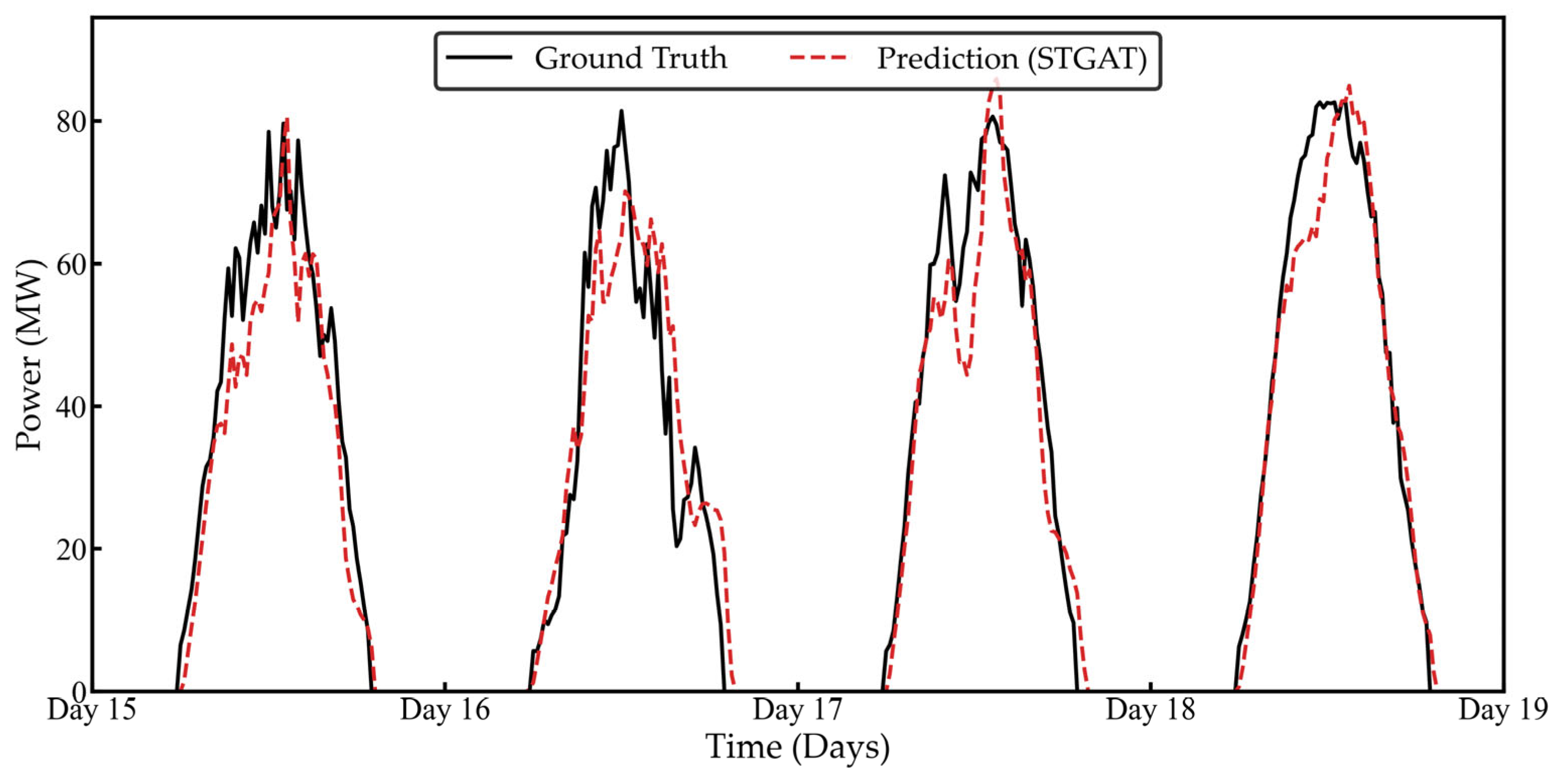
Considering the diurnal nature of PV output, predicting only the next 4 h at an ultra-short timescale cannot fully capture the daily PV output pattern. This study first performs short-term PV output forecasting for the next day, generating a 96-step-ahead forecast. The resulting point forecasts are shown in Figure 6.

As shown in Figure 6, the STGAT model accurately captures the daily variation patterns of PV power output, precisely tracking the rapid climb in the early morning, sustained peak during midday, and abrupt drop in the evening. Notably, even during periods of intense power fluctuations caused by cloud cover, the model’s prediction curve remains highly consistent with actual values. This demonstrates that the spatio-temporal attention mechanism effectively integrates collaborative information from neighboring stations, significantly enhancing adaptability to abrupt operational changes. Furthermore, the model demonstrates outstanding stability in multi-day forecasts, with peak prediction errors controlled within 2%, validating its long-term modeling capability.

To comprehensively evaluate model performance, ultra-short-term forecasts extending 4 h ahead were conducted. The error metrics RMSE and MAE for 4 h and 1-day forecasts across the entire dataset are presented in

Table 3. Overall dataset point prediction error.

Evaluation Indicators	4 h (Ahead)	1 d (Ahead)
RMSE	5.2570%	14.0591%
MAE	2.3685%	6.1984%

.

The data in Table 3 indicate that the prediction time scale significantly impacts model accuracy. For 4 h lead forecasts, the RMSE and MAE were 5.2570% and 2.3685%, respectively, while 1-day lead forecasts saw errors increase to 14.0591% and 6.1984%, representing relative error increases of approximately 8.8% and 4.3%. This discrepancy stems from the cumulative effect of meteorological uncertainty during extended forecasting periods. Nevertheless, even within a 24 h prediction window, the model maintains MAE below 7% and RMSE under 15%, fully demonstrating the QR-STGAT architecture’s robust modeling capability for complex spatio-temporal dependencies.

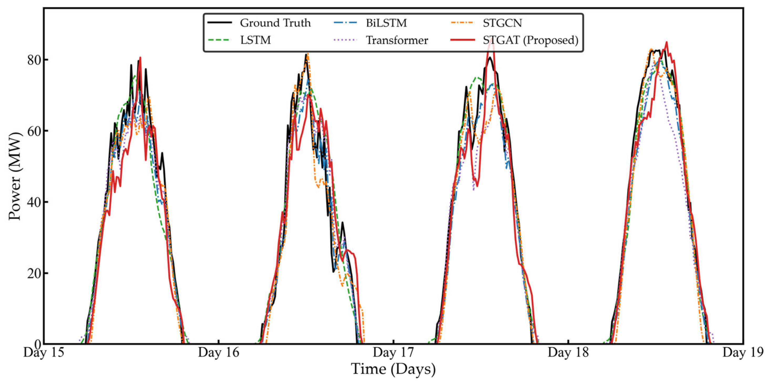
To validate the effectiveness of the proposed PV power forecasting method, the point forecasting model based on QR-STGAT was further compared with models based on LSTM, BiLSTM, and Transformer, as shown in Figure 7 and

Table 4. Comparison of Prediction Errors Among Different Algorithms in One-Day-Ahead Forecasts.

Method	RMSE (MW)	MAE (MW)
QR-STGAT	14.0591	6.1984
Transformer	21.1464	11.3349
STGCN	17.6120	9.2536
LSTM	25.6734	13.8907
BiLSTM	26.0484	14.0291

. As evident from Figure 7, the photovoltaic power prediction curve generated by the proposed method exhibits the highest degree of alignment with actual values. Particularly during periods of intense power fluctuations (such as the cloud disturbance period from 12:00 to 14:00), the STGAT model accurately tracks sudden power changes, whereas LSTM and BiLSTM models exhibit noticeable lag and deviation. Although the Transformer model possesses parallel computing advantages, its response to short-term sudden changes is slower than that of STGAT.

Further analysis of Table 4 reveals that under equivalent conditions, the QR-STGAT model achieves a prediction accuracy of 93.48%, with RMSE and MAE values of 14.0591 MW and 6.1984 MW, respectively. Compared to the traditional LSTM model, the RMSE improved by 11.61% and MAE by 11.99%; compared to BiLSTM, the RMSE improved by 10.38% and MAE by 10.72%; and compared to Transformer, the RMSE improved by 9.52% and MAE by 9.87%. Importantly, QR-STGAT also outperforms the graph-based spatial baseline STGCN, achieving an RMSE improvement of 20.17% and an MAE improvement of 33.07% over STGCN. This result demonstrates that the adaptive attention-based spatial aggregation in QR-STGAT captures inter-station dependencies more effectively than the fixed-weight graph convolution used in STGCN, thereby validating the specific added value of the proposed spatial modeling approach. This significant overall performance improvement stems from: (1) the graph attention mechanism dynamically capturing nonlinear correlations between sites, overcoming the limitation of fixed spatial weights in STGCN and the single-site temporal modeling constraint of LSTM-based methods; (2) the spatiotemporal joint modeling architecture simultaneously extracting spatial dependencies and temporal evolution patterns, which neither BiLSTM nor Transformer can achieve due to their lack of spatial topology integration; (3) the quantile regression loss function enhancing robustness against abnormal operating conditions. Collectively, these findings demonstrate that the proposed method exhibits superior generalization capabilities and disturbance resistance in complex spatiotemporal coupling scenarios.

To verify that the performance improvements of the proposed QR-STGAT model over the baseline models are statistically meaningful rather than attributable to random variation in training, the Diebold–Mariano (DM) test was conducted. The DM test is a standard statistical tool for comparing the predictive accuracy of two forecasting models based on their loss differentials. A negative DM statistic indicates that the forecast errors of QR-STGAT are significantly smaller than those of the corresponding baseline, and a p-value below 0.01 indicates that this difference is statistically significant at the 1% level.

As shown in

Table 5. Diebold–Mariano Test Results for Statistical Significance of Forecast Improvements.

Comparison (Proposed vs. Baseline)	DM Statistic	p-Value
QR-STGAT vs. LSTM	−6.7587	<0.01
QR-STGAT vs. BiLSTM	−3.7650	<0.01
QR-STGAT vs. Transformer	−3.0761	<0.01
QR-STGAT vs. STGCN	−5.9227	<0.01

Note: A negative DM statistic indicates that the forecast errors of QR-STGAT are significantly smaller than those of the corresponding baseline model. All comparisons are statistically significant at the 1% level (p < 0.01).

, the DM statistics for QR-STGAT against all four baseline models are negative, with values of −6.7587, −3.7650, −3.0761, and −5.9227 against LSTM, BiLSTM, Transformer, and STGCN, respectively. All p-values are below 0.01, indicating that the improvements are statistically significant at the 1% level across all comparisons. These results confirm that the superior forecasting performance of QR-STGAT is not attributable to random variation in training, but reflects a genuine and statistically robust improvement over existing temporal and spatial baseline models.

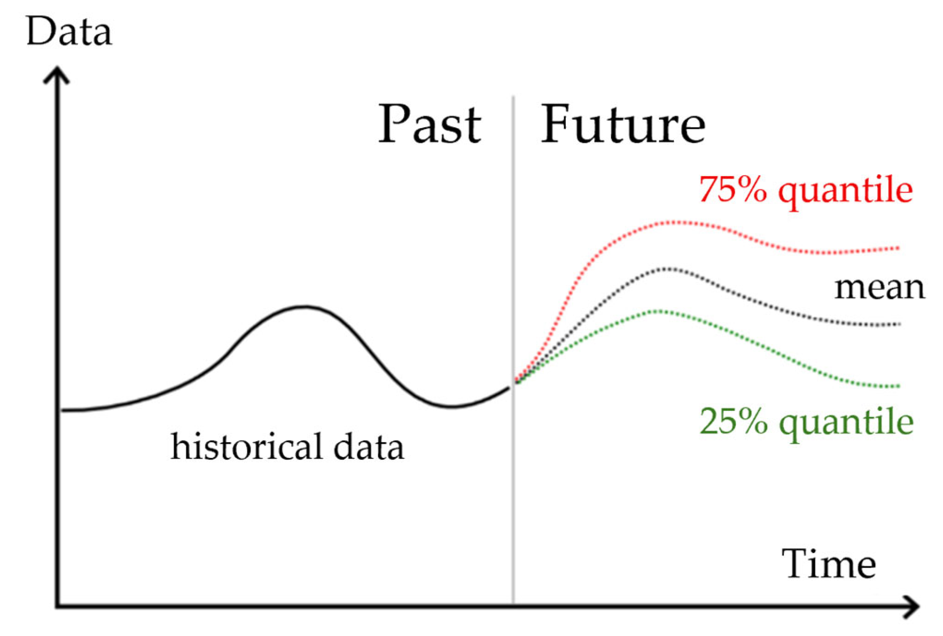
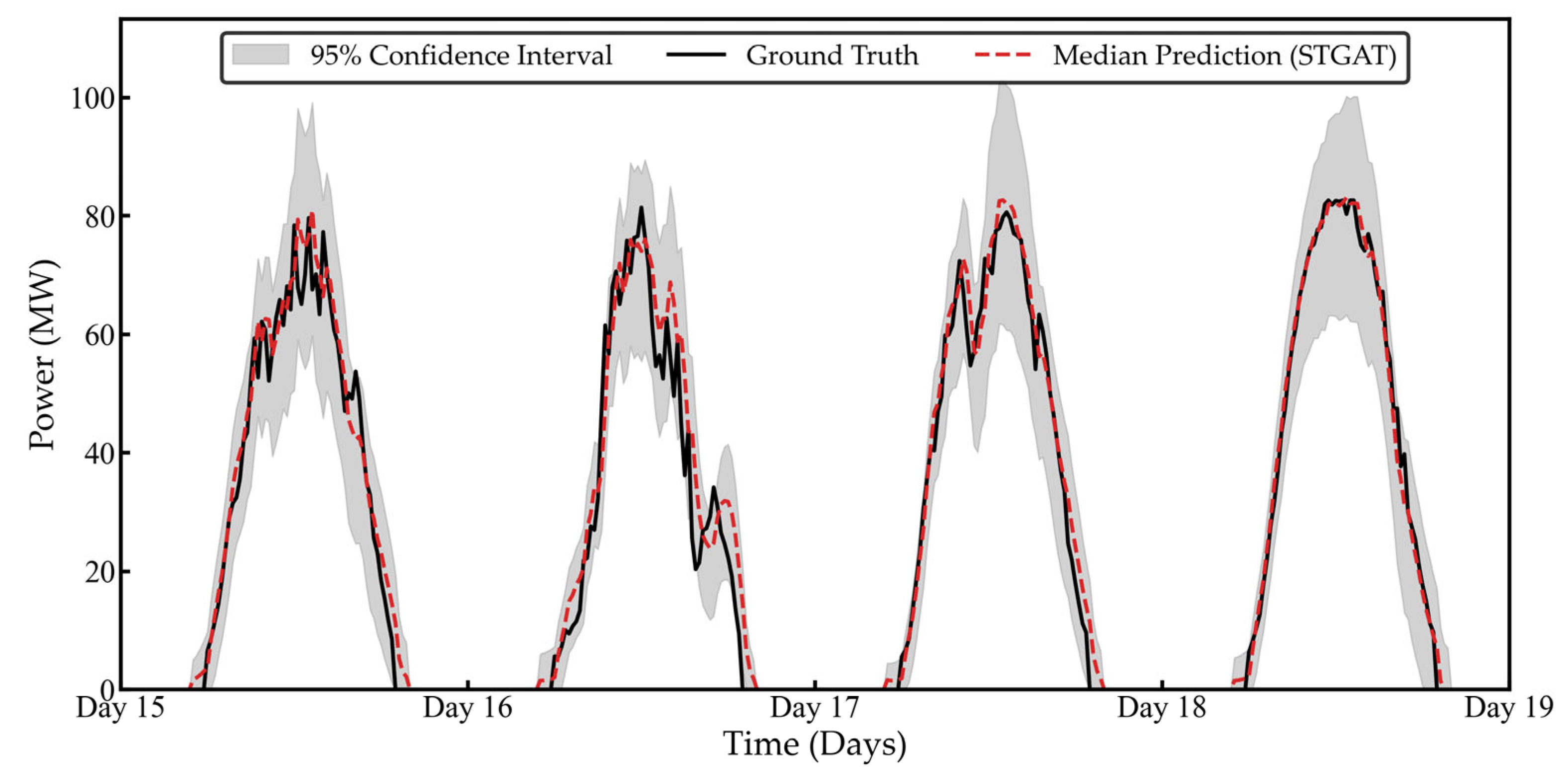
Given the limitations of point forecasting, confidence intervals are calculated by combining quantile results with different confidence levels. The calculations indicate that the best fit between predicted and actual values occurs when the quantile is set to 0.5. When a 95% confidence interval is applied, the resulting probability forecast range is shown in Figure 8. The figure clearly demonstrates that the prediction interval widens during periods of significant power fluctuations and narrows during stable conditions. This behaviour is consistent with the expected properties of probabilistic forecasting, where uncertainty grows with power variability. The adaptive interval width reflects the model’s robustness to meteorological disturbances, providing reliable uncertainty bounds for grid dispatch decisions.

The probability prediction evaluation metrics under different confidence intervals are shown in

Table 6. One-Day-Ahead Probability Interval Forecast Evaluation Indicator.

Evaluation Metric	90% Confidence Interval	95% Confidence Interval
RMSE	14.0034	13.9350
MAE	6.0069	6.0504
PICP	88.7819%	93.0518%
PINRW	0.0481	0.0561
CWC	19.4801	14.6579

. Increasing the confidence level requirement elevated the prediction interval coverage probability (PICP) from 88.78% to 93.05%, while the prediction interval normalized width (PINRW) increased from 0.0481 to 0.0561. The composite score (CWC) improved from 19.4801 to 14.6579. This pattern aligns with fundamental probability prediction characteristics: expanding the confidence interval trades a broader prediction range for higher coverage probability, thereby enhancing prediction reliability. Notably, point prediction error metrics RMSE and MAE remain largely stable across confidence levels, maintaining around 14% and 6%, respectively. This indicates that confidence interval adjustments primarily affect the precision of uncertainty quantification while having minimal impact on deterministic prediction accuracy.

To further quantify the impact of the static graph topology on model performance under varying meteorological conditions, an additional weather-stratified error analysis was conducted. The test set was partitioned into three weather categories based on daily physical characteristics, including daily maximum power output and first-order variability rate: sunny days, cloudy/abrupt-change days, and rainy/overcast days. Point prediction metrics (RMSE, MAE) are normalised by the daily maximum power output to ensure fair comparison across conditions with different absolute output scales. Probabilistic metrics (PICP, PINRW) are also reported. Results are presented in

Table 7. Performance of QR-STGAT Under Different Meteorological Conditions.

Weather Condition	RMSE (%)	MAE (%)	PICP (%)	PINRW
Sunny	27.22	15.60	93.57	0.0597
Cloudy/Abrupt Change	27.04	15.85	93.84	0.0518
Rainy/Overcast	36.55	20.96	88.96	0.0631

Note: RMSE and MAE values are normalised by the daily maximum power output (%) to ensure fair comparison across weather conditions with different absolute output scales. Weather categories are determined based on the daily maximum power output and the first-order variability rate of the test set.

.

As shown in Table 7, the model performs consistently well under sunny and cloudy/abrupt-change conditions, with RMSE values of 27.22% and 27.04%, respectively, and PICP values above 93%. However, under rainy and overcast conditions, RMSE increases to 36.55% and PICP drops to 88.96%, falling below the nominal 90% coverage target. This performance degradation is attributable to the static nature of the adjacency matrix. Under heavy cloud cover and localised precipitation, the instantaneous spatial correlation structure among PV stations deviates substantially from the historical average encoded in the fixed graph topology, leading to misspecified spatial aggregation weights and reduced accuracy in both point prediction and interval coverage. This finding provides empirical support for the limitation acknowledged in the Conclusions and further motivates the adoption of a dynamic graph construction mechanism in future work.

6. Conclusions

To more accurately describe the correlation between regional photovoltaic outputs and characterize the uncertainty of photovoltaic generation, this paper proposes a probabilistic forecasting method based on spatio-temporal graph attention networks and quantile regression. This method constructs a spatial graph topology of PV power plants, employs a graph attention mechanism to adaptively learn spatial correlation weights between different plants, utilizes a convolutional neural network to extract multidimensional meteorological features, and captures temporal dependencies through gated recurrent units. Building upon this foundation, a quantile regression approach is introduced to construct prediction intervals, achieving a transition from point prediction to probabilistic forecasting. Key findings are as follows:

• The Spatio-Temporal Graph Attention Network effectively captures spatial dependencies among regional PV installations by constructing the topological structure of PV power plant graphs and adaptively learning spatial weights. Case study results demonstrate that the proposed QR-STGAT model achieves a prediction accuracy of 93.48% for one-day-ahead forecasts. Compared to traditional methods modeling only single-site time series, QR-STGAT reduced RMSE by 11.61%, 10.38%, and 9.52% relative to LSTM, BiLSTM, and Transformer, respectively, with corresponding MAE reductions of 11.99%, 10.72%, and 9.87%. This fully validates the effectiveness of spatial topology modeling and graph attention mechanisms in regional PV power forecasting.
• The quantile regression-based probabilistic forecasting method quantifies PV output uncertainty, providing more comprehensive decision support for grid dispatch. Experiments demonstrate that at a 95% confidence level, the probability of interval coverage (PICP) reaches 93.05%, with a normalized interval width (PINRW) of 0.0561. The prediction interval adapts dynamically to power fluctuations, automatically widening during periods of extreme power variation to maintain coverage, reflecting the model’s robust disturbance resistance.
• This study employs a static graph topology construction method based on geographic distance and power correlation, which does not fully account for the dynamic impact of weather conditions on spatial correlations between power plants. Future research may incorporate dynamic graph learning mechanisms to adaptively update the adjacency matrix based on meteorological conditions and temporal features. Additionally, exploring multi-scale spatiotemporal modeling strategies could further enhance the model’s generalization performance across diverse weather scenarios.