Energy Performance of Thermocable-Assisted SAGD for Heavy Oil Reservoirs: Heat-Loss Mitigation, Steam Chamber Development, and SOR Reduction

Abstract

Steam-assisted gravity drainage (SAGD) remains one of the most effective thermal enhanced-oil-recovery technologies for heavy-oil reservoirs; however, its energy performance is strongly constrained by wellbore heat losses, delayed steam-chamber development, and an increase in the steam–oil ratio (SOR) under deep or thermally unfavorable conditions. This study develops a physics-based computational digital-twin framework for thermocable-assisted SAGD and evaluates the influence of steam temperature, oil viscosity, permeability, reservoir depth, thermocable linear power, and heating time on oil production and SOR. The model couples wellbore heat transfer, temperature-dependent viscosity reduction, steam-chamber geometry, heat-loss compensation by an electrical thermocable, and production response. The results show that increasing steam temperature from 220 to 300 °C raises the oil rate by approximately 13–15% and reduces SOR from about 2.47 to 2.30. Increasing oil viscosity from 300 to 1500 mPa·s decreases the oil rate by more than 25% and increases SOR above 3.0. Thermocable integration increases the oil rate by approximately 8–12% in the base scenario and reduces SOR by 5–10% compared with conventional SAGD. The highest relative benefit is obtained in deeper reservoirs, where additional heat input compensates wellbore heat losses and stabilizes the temperature profile. These findings indicate that thermocable-assisted SAGD can improve energy efficiency and extend the practical operating window of thermal recovery in heavy-oil reservoirs.

1. Introduction

The development of heavy-oil and bituminous-sand reservoirs remains one of the most challenging tasks in modern petroleum engineering. The difficulty is caused by the extreme rheological properties of the hydrocarbons, the strong temperature dependence of viscosity, and the need to apply energy-intensive recovery methods. Unlike conventional light oils, heavy oils may exhibit viscosities of hundreds or thousands of mPa·s under reservoir conditions, which makes efficient production impossible without external thermal stimulation. For this reason, thermal enhanced oil recovery (thermal EOR) has become a central technological pathway for the exploitation of such resources [1,2,3].

Recent studies on deep extra-heavy-oil SAGD, electrical preheating, and downhole heating further confirm that heavy-oil recovery efficiency depends strongly on heat delivery, steam quality, viscosity reduction, and the location of auxiliary heat supply [4,5,6].

Among the existing thermal technologies, steam-assisted gravity drainage (SAGD) has achieved wide industrial application, especially in shallow heavy-oil deposits and oil sands. In the classical SAGD configuration, saturated steam is injected through an upper horizontal well, forming a steam chamber that expands upward and laterally. The heated oil loses viscosity and drains under gravity toward a lower producer. Although SAGD has proven effective under favorable geological conditions, its performance is constrained by heat losses, reservoir depth, steam quality deterioration, and the time required to establish thermal communication between the injector and the producer [1,7,8].

The heat balance of the SAGD system is one of the most important factors controlling process efficiency. It includes heat transfer from steam to oil, heat loss along the wellbore, heat exchange with the surrounding formations, and heat storage in the rock-fluid system. As reservoir depth increases, the thermal path from the surface to the productive interval becomes longer. This leads to greater heat dissipation during steam transport and reduces the effective temperature delivered to the reservoir. Consequently, the downhole steam quality and thermal potential decrease, the steam chamber grows more slowly, and oil rate declines. This effect becomes especially critical at depths exceeding approximately 800–1000 m, where classical SAGD may demonstrate poorer production performance and a higher steam–oil ratio (SOR) [8,9,10].

Several published SAGD studies and field-scale analyses show that the deterioration of thermal performance with increasing depth is not only qualitative, but also measurable. With increasing vertical depth, the steam transport path becomes longer, the cumulative wellbore heat loss increases, and the effective heat delivered to the reservoir interval decreases. As a result, deeper SAGD projects commonly require higher steam injection energy and longer start-up or preheating periods, and may exhibit higher SOR compared with shallow oil–sand applications. Reported SAGD operations typically show SOR values in the range of approximately 2–5 depending on oil viscosity, permeability, reservoir thickness, steam quality, and operating strategy, while thermally unfavorable or deeper reservoirs may approach the upper part of this range. These quantitative observations support the need for auxiliary downhole heating methods that can compensate for part of the heat deficit near the reservoir interval and improve early thermal communication between the injector and producer [4,5,6,8,9,10].

A second limitation of SAGD in deeper or colder reservoirs is delayed start-up. During the early stage of operation, the interwell region must be heated sufficiently to create hydraulic and thermal communication between the injector and producer. If wellbore heat losses are high and the bottom-hole steam temperature is insufficient, the start-up time increases substantially. This results in additional energy consumption and may reduce the economic attractiveness of the project. In some cases, start-up may become technically difficult without auxiliary heating methods.

A number of approaches have been studied to overcome these limitations and improve the thermal efficiency of SAGD. These include vacuum insulated tubing (VIT), solvent-assisted SAGD, optimization of steam injection parameters, flow-control completions, electrical heating, and electromagnetic heating. Each method has advantages but also important constraints. VIT reduces heat losses but cannot eliminate them completely, especially at large depths. Solvent-assisted processes may reduce viscosity and steam demand, but they introduce phase-behavior complexity, solvent recovery issues, and additional costs. Electromagnetic methods can deliver heat to the reservoir but may require complex equipment and significant electrical energy [11,12,13].

Recent studies further confirm that subsurface thermal stimulation is controlled not only by the total amount of supplied heat, but also by heat-source location, heating duration, and thermal cycling. Thermal-stimulation studies in deep geothermal reservoirs have shown that repeated heating changes the thermo-mechanical state of the rock and can influence fracture evolution and heat-transfer pathways [14]. Heating-cooling experiments on granite also demonstrate that cyclic temperature loading can modify mechanical properties and damage evolution [15]. For heavy-oil recovery, electrical preheating studies for SAGD well pairs have shown that heater deployment and preheating strategy can affect temperature distribution, start-up behavior, and subsequent recovery performance [16]. These findings support the need to compare different thermocable arrangements and heating-mode scenarios in the present study.

In this context, downhole electrical heating systems, particularly thermocables, represent a promising option. A thermocable provides local and distributed electrical heating directly along the wellbore or near the productive interval. Unlike passive thermal insulation, a thermocable actively compensates for heat losses and can maintain a more favorable temperature regime along the horizontal section. This is especially relevant in deeper heavy-oil reservoirs, where conventional SAGD becomes less effective due to steam cooling before the heat reaches the drainage zone.

The relevance of this approach is also supported by previous studies on electrical heating, downhole heaters, and electrical preheating for heavy-oil recovery and SAGD start-up. These studies indicate that a localized electrical heat supply can reduce near-wellbore oil viscosity, shorten the time required to establish thermal communication, and improve the uniformity of the early temperature field around the well pair. Although the specific design of electrical heaters, heating cables, and power-delivery systems differs between studies, their common engineering role is to supply heat closer to the reservoir interval than surface-generated steam alone. Therefore, thermocable-assisted SAGD is considered here not as a replacement for steam injection, but as an auxiliary heat-loss mitigation and start-up support technology [4,5,6,16,17,18,19,20].

The integration of thermocables with SAGD opens new possibilities for controlling the thermal regime of the reservoir. Additional heat supplied near the bottom-hole region and along the horizontal section can accelerate reservoir warm-up, promote earlier steam-chamber formation, reduce oil viscosity in the critical drainage zone, and increase oil rate. Active heating can also reduce the sensitivity of the process to unfavorable initial conditions and improve stability under variable steam-injection parameters.

However, the application of thermocables in SAGD requires a detailed analysis of the coupled thermal processes in the wellbore-reservoir system. Key questions include the extent to which the thermocable compensates for heat losses, its effect on the temperature profile along the wellbore, the impact of additional heat input on steam-chamber dynamics, and the resulting changes in SOR and energy efficiency [21,22].

The temperature distribution and heat-flux pattern are particularly important because they determine the effectiveness of reservoir heating and oil drainage. With thermocable assistance, the temperature field may become more uniform, reducing underheated zones and promoting more stable steam-chamber growth. This improves the utilization of thermal energy and can reduce the specific energy demand per unit of produced oil.

Thermocable heating also modifies the energy efficiency of SAGD. In the classical configuration, a significant part of the supplied heat is lost during steam transport. When downhole electrical heating is added, part of the energy is supplied directly near the production zone. This redistributes the energy flows in the system and can potentially reduce the steam requirement per unit of produced oil. A realistic assessment must consider both the additional electrical power and the reduction in steam consumption.

Reservoir depth is another important aspect. As depth increases, wellbore heat losses become more severe and the value of active downhole heating becomes greater. Thermocable-assisted SAGD can therefore be interpreted as a method for extending the applicability of SAGD toward deeper reservoirs that would otherwise be marginal or uneconomic under conventional thermal recovery.

Although several studies have considered electrical heating in heavy-oil reservoirs, an integrated analysis of thermocable-assisted SAGD for deep reservoirs remains insufficiently developed. In particular, there is a lack of systematic studies that combine heat transfer, steam-chamber development, SOR behavior, heat-loss compensation, and energy efficiency within one unified computational framework. This gap motivates the development of an integrated model capable of evaluating the influence of geological, thermophysical, and operational parameters on process performance.

The research gap addressed in this study is the lack of a transparent engineering-screening framework that simultaneously links wellbore heat loss, thermocable heat compensation, temperature-dependent viscosity reduction, steam-chamber evolution, SOR behavior, and energy-performance indicators for deep heavy-oil SAGD conditions. Previous studies have considered SAGD heat transfer, electrical heating, or steam-chamber behavior separately, but an integrated comparison of classical SAGD and thermocable-assisted SAGD under depth-dependent heat-loss conditions remains limited.

The novelty of this work is the integrated coupling of thermocable heat-loss compensation with SAGD production and energy-performance indicators in a physics-informed computational workflow. The model is not intended to replace a field-calibrated commercial simulator; instead, it provides a transparent tool for preliminary design, scenario ranking, and interpretation of how auxiliary downhole heating changes SAGD performance under thermally unfavorable conditions.

The objective of this study is to analyze the efficiency of thermocable-assisted SAGD for heavy-oil reservoirs, with emphasis on heat transfer, steam-chamber formation, production response, and energy indicators. The study considers several development scenarios, including classical SAGD, SAGD under increased reservoir depth, and SAGD with distributed downhole heating. Numerical experiments are used to identify the key factors controlling oil rate and SOR.

The main objectives of the study are to quantify wellbore heat losses at different depths, evaluate the effect of thermocable heating on temperature distribution, analyze steam-chamber evolution, assess oil-rate and SOR responses, and rank the key input parameters through sensitivity analysis. Particular attention is given to the quantitative effect of active heating on heat-loss compensation and oil-rate improvement.

The practical significance of the research is related to the possibility of using the proposed workflow for preliminary screening of thermocable-assisted SAGD under different geological and operating conditions. The results can support early-stage selection of thermocable power, heating duration, arrangement strategy, and depth-dependent operating scenarios before detailed field-calibrated simulation or pilot testing.

The calculations were performed using a computational model implemented in Python. The model combines heat transfer and filtration relationships, temperature-dependent viscosity reduction, wellbore heat-loss modeling, steam-chamber geometry, and additional heat supplied by the thermocable. The flexible implementation allows systematic numerical experiments for different reservoir and operating conditions and supports future extension toward field-calibrated digital-twin workflows.

2. Materials and Methods

This study considers the problem of improving heavy-oil recovery using SAGD under increased reservoir depth. The emphasis is placed on heat transfer, wellbore heat loss, steam-chamber growth, and the influence of additional downhole electrical heating provided by a thermocable [23,24,25,26].

The model is based on the coupling of thermal and filtration processes in a wellbore-reservoir system. The main modeled components are as follows:

• heat transfer in the wellbore;
• heat exchange with surrounding rock;
• temperature-dependent oil viscosity reduction;
• gravity-driven filtration of heated oil;
• formation and expansion of the steam chamber;
• additional distributed heat input from the thermocable.

Stationary and quasi-stationary regimes are considered to estimate the evolution of the system over time and to compare different operating scenarios. The classical SAGD concept is based on the Butler theory, in which a steam chamber forms above the injector and heated oil drains under gravity toward the producer. Modern heavy-oil development conditions require extensions of this classical framework to include complex well geometry, wellbore heat losses, auxiliary heat sources, and computational analysis suitable for digital monitoring.

The proposed physics-informed computational digital twin of thermocable-assisted SAGD integrates steam thermodynamics, heat transfer, well geometry, steam-chamber growth, and production prediction. The following subsections describe the model components used in the numerical experiments.

2.1. Steam Heat Input and Wellbore Heat Losses

The heat balance of the steam stream is used as the starting point of the model. The thermal power supplied by steam is expressed as

$$Q_{steam}=\dot{m}\cdot h_{steam},$$

(1)

where $Q_{steam}$ is the steam heat flow rate (W), $\dot{m}$ is the mass flow rate of steam (kg/s), and $h_{steam}$ is the specific enthalpy of steam (J/kg). For engineering calculations, the steam enthalpy is approximated as

$$h_{steam}=2000+3.8(T_{steam}-120),$$

(2)

This approximation avoids the need for complex steam-table calculations while preserving numerical stability and sufficient accuracy for comparative engineering simulations. The heat loss along the wellbore is represented by two main contributions: heat loss into the surrounding rock and heat loss through the pipe wall:

$$Q_{loss}=Q_{rock}+Q_{pipe},$$

(3)

where $Q_{\mathrm{loss}}$ is the total heat loss from the wellbore system, W; $Q_{\mathrm{rock}}$ is the heat loss from the wellbore to the surrounding rock formation, W; and $Q_{\mathrm{pipe}}$ is the heat loss through the pipe wall and wellbore completion elements, W.

The heat loss to the surrounding rock is based on radial heat conduction in cylindrical coordinates [26]:

$$Q_{rock}={\displaystyle \frac{2\pi \lambda L}{\mathrm{l}\mathrm{n}(r_{out}/r_{in})}},$$

(4)

where $\lambda$ is the thermal conductivity of the formation, $L$ is the length of the considered wellbore segment, and $r_{in}$ and $r_{out}$ are the inner and outer radii of the heat-transfer domain. The pipe-related heat loss is represented as

$$Q_{pipe}={\displaystyle \frac{2\pi L}{\delta \cdot k_{pipe}}},$$

(5)

where $\delta$ is the wall thickness and $k_{pipe}$ is the effective heat-transfer coefficient of the pipe system. These equations provide a baseline estimate of heat loss and are extended below to represent nonlinear reservoir and operating effects.

Equations (1)–(5) are based on standard engineering heat-balance and radial-conduction approximations commonly used for wellbore heat-transfer and thermal-recovery screening calculations [23,24,25,26,27].

In Equations (4) and (5), the temperature-driving effect is introduced through the extended heat-loss scaling terms in Equation (6), which include steam temperature, reservoir properties, geometry, and heating time.

2.2. Extended Heat-Loss Formulation

Classical analytical heat-transfer models often assume stationary conditions and homogeneous media. Actual SAGD operations are more complex because heat loss depends on steam temperature, reservoir depth, oil viscosity, flow regime, heating time, and the geometry of the wellbore-reservoir system. To account for these effects, an extended heat-loss formulation is introduced [27]:

$$Q_{loss}^{eff}=C_{th}\cdot L\cdot {\mathsf{\Phi }}_{steam}\cdot {\mathsf{\Psi }}_{geo}\cdot {\mathsf{\Theta }}_{res}\cdot {\mathsf{\Omega }}_{time}\cdot (1-{\beta }_{cable}),$$

(6)

where $C_{th}$ is an effective heat-transfer coefficient, ${\mathsf{\Phi }}_{steam}$ = f(T_steam) describes the influence of steam temperature, ${\mathsf{\Psi }}_{geo}$ = f(H,z,L) is the geometric factor reflecting depth and length effects, ${\mathsf{\Theta }}_{res}$ = f(μ,φ) describes reservoir and fluid properties, ${\mathsf{\Omega }}_{time}$ = f(t) is the time factor, and ${\beta }_{cable}$ is the thermocable compensation coefficient.

This form recognizes that heat loss is not controlled by geometry or thermal conductivity alone. It is also affected by oil rheology, steam rate, the temperature gradient between steam and reservoir, and the duration of heating. Increasing oil viscosity reduces fluid mobility, localizes heat distribution, and may increase local thermal gradients. Increasing the steam rate raises the absolute thermal input, but relative heat loss may increase or decrease depending on flow and heat-distribution conditions. The extended function therefore allows nonlinear scaling of heat losses, including overheating effects at high steam rates, degradation of thermal efficiency at high viscosity, and stabilization during longer heating periods.

2.3. Thermal Efficiency Coefficient

The thermal efficiency coefficient is a key indicator of how much supplied steam energy contributes to reservoir heating and viscosity reduction [28]. In the classical form, it is calculated as

$$\eta ={\displaystyle \frac{Q_{steam}-Q_{loss}}{Q_{steam}}},$$

(7)

This expression represents the fraction of steam energy effectively used in the reservoir. However, in actual SAGD operations, efficiency is influenced by multiple geological and operating factors, including reservoir geometry, rock-fluid properties, and well operating regime [29,30]. Therefore, the following extended formulation is used:

$$\eta ={\eta }_0\cdot f_1\left(z\right)\cdot f_2\left(\mu \right)\cdot f_3\left(\varphi \right)\cdot f_4\left(h\right)\cdot f_5\left(P\right),$$

(8)

where $f_1(z$) represents the effect of depth, $f_2(\mu$) the effect of viscosity, $f_3(\varphi$) the effect of porosity, $f_4(h$) the effect of reservoir thickness, and $f_5(P$) the effect of reservoir pressure. This formulation treats SAGD efficiency as an integrated system property rather than a constant. For example, greater depth increases wellbore heat losses, higher porosity can improve heat distribution, and reservoir thickness can either support or limit chamber development depending on the growth regime.

2.4. Thermocable Effect

The thermocable is introduced into the model as an additional distributed heat source that reduces effective heat losses and stabilizes the temperature field along the wellbore. Its effect is represented by the compensation factor [17,18,19,20]:

$${\beta }_{cable}=1-\mathrm{e}\mathrm{x}\mathrm{p}\left(-\gamma \cdot {\displaystyle \frac{P_c\cdot L_{cable}\cdot {\eta }_c}{Q_{ref}}}\right),$$

(9)

where $L_{cable}$ is cable length, $P_c$ is linear power, ${\eta }_c$ is heat-transfer efficiency, $\gamma$ is an empirical coefficient, and $Q_{ref}$ is a characteristic reference heat flow. Physically, ${\beta }_{cable}$ expresses the ability of the cable to compensate heat losses and maintain the required thermal regime along the wellbore. The heat-loss term is then modified as

$$Q_{loss}^{new}=Q_{loss}\cdot (1-{\mathsf{\beta }}_{cable}),$$

(10)

where $Q_{\mathrm{loss}}^{\mathrm{new}}$ is the corrected heat loss after accounting for thermocable assistance, W; $Q_{loss}$ is the initial heat loss without thermocable compensation, W; and ${\beta }_{cable}$ is the thermocable heat-loss compensation coefficient, dimensionless.

The thermocable does more than reduce heat loss. It changes the shape of the temperature field by increasing the length of the heated zone, decreasing local temperature gradients, and stabilizing the front of the steam chamber. This transition from classical SAGD to a hybrid thermo-electric thermal process is one of the central elements of the model.

In the numerical implementation, the thermocable effect is not introduced as a constant production multiplier. It is calculated as a bounded nonlinear factor controlled by the active cable length, linear power, temperature set point, heat-transfer efficiency, coverage of the horizontal section, horizontal-well length, and steam temperature. This formulation reflects the engineering assumption that a short or low-power cable cannot compensate wellbore heat losses to the same extent as a cable that covers most of the horizontal interval and operates with higher thermal efficiency. The resulting factor is then used to reduce effective heat losses and to modify the wellbore temperature profile, SOR, oil-rate response, and steam-chamber growth.

2.5. Temperature Distribution Along the Wellbore

Temperature distribution along the wellbore controls the effectiveness of heat delivery to the reservoir. The model uses an exponential cooling relationship:

$$T\left(s\right)=T_{res}+(T_{in}-T_{res})e^{-s/L_{cool}},$$

(11)

where $T\left(s\right)$ is the steam or wellbore temperature at distance $s$, °C; $T_{res}$ is the initial reservoir temperature, °C; $T_{in}$ is the inlet steam temperature at the beginning of the considered wellbore section, °C; $s$ is the distance along the wellbore, m; and $L_{cool}$ is the characteristic cooling length, m. This cooling length is not treated as a constant; instead, it depends on thermal efficiency and the presence of the cable:

$$L_{cool}=f(\eta ,cable),$$

(12)

Thus, an increase in process efficiency or the use of a thermocable increases the effective thermal-front length and produces more uniform heating along the horizontal section. The wellbore-temperature profile therefore responds adaptively to operating conditions.

The exponential temperature-decay formulation in Equation (11) should be interpreted as a reduced-order engineering approximation. It assumes that the heat-transfer medium around the wellbore can be represented by effective homogeneous thermal properties. In heterogeneous reservoirs, shale streaks, permeability barriers, anisotropic thermal conductivity, variable water saturation, local facies changes, and non-uniform steam distribution can distort the temperature front and produce deviations from a simple exponential profile. Therefore, Equation (11) is not intended to replace a fully heterogeneous thermal reservoir simulator. In the present study, it is used to capture the dominant first-order cooling trend along the wellbore and to compare relative differences between conventional SAGD and thermocable-assisted SAGD under controlled parameter variations.

2.6. Steam-Chamber Development and Reservoir Temperature Field

Steam-chamber formation is the central mechanism of SAGD. In classical Butler-type theory, chamber growth is governed by the balance between heat transfer and gravity drainage [7,21]. In the present model, chamber height and width are treated as functions of thermal efficiency, heating time, and SOR:

H = H₀⋯f(η, t, SOR), W = W₀⋯f(η, t, SOR).

High thermal efficiency accelerates chamber growth, low SOR indicates efficient heat utilization, and longer heating time leads to a saturation-type expansion. The model also accounts for unfavorable behavior at high SOR, where inefficient heating may limit chamber expansion.

The reservoir temperature field is generally described as

$$T(x,y,z)=T_{res}+f(\eta ,t,SOR,cable),$$

(13)

The temperature field is non-uniform: maximum temperatures occur near the chamber roof and close to the heated wellbore, while temperature decreases away from the chamber center and forms a gradual thermal halo [29]. The model uses an elliptical chamber geometry, spatial gradients, and temporal evolution to represent this behavior.

2.7. SOR and Production Model

The steam–oil ratio is a key performance indicator for SAGD and is defined as [17,18,30]

$$SOR={\displaystyle \frac{Q_{steam}}{Q_{oil}}},$$

(14)

Q_oil = Q_steam/SOR

Rather than prescribing SOR empirically, the proposed digital twin calculates it as a result of the thermal state, reservoir properties, steam-chamber geometry, and thermocable effect:

$$SOR=f(\eta ,\mu ,k,T,cable),$$

(15)

Oil production is therefore not imposed as an external empirical value, but arises from the interaction of heat transfer, viscosity reduction, geometry, and drainage efficiency. The overall integrated production operator is written as

$$Q_{oil}=\mathcal{F}(Q_{steam},\mu ,geometry,t,{\beta }_{cable}),$$

(16)

This formulation links heat transfer, temperature field, viscosity reduction, SOR, and oil production into one computational workflow. In contrast to conventional models that treat these processes separately, the proposed system enables feedback between thermal and production variables and is suitable for scenario analysis.

The SOR formulation combines physical heat-balance reasoning with semi-empirical correction factors. It was not calibrated against a specific field-history-matched SAGD dataset; therefore, the calculated SOR values should be interpreted as comparative engineering estimates rather than direct field forecasts. To avoid overstatement, the model is used in this study to evaluate relative trends caused by changes in steam temperature, oil viscosity, permeability, reservoir depth, and thermocable heating. The credibility of the SOR response is supported by physical trend consistency, grid/time-step convergence, and comparison with published SAGD operating ranges. In the investigated cases, the calculated SOR values remain within the typical engineering range reported for SAGD applications under heavy-oil conditions, while unfavorable cases with higher viscosity or greater heat loss shift toward the upper part of this range.

Figure 1 illustrates the simplified computational workflow of the proposed thermocable-assisted SAGD screening model [31,32,33,34]. The workflow begins with input parameters describing reservoir properties, fluid characteristics, wellbore geometry, steam-injection conditions, and thermocable design. These inputs are used to estimate steam heat input, wellbore heat loss, thermocable heat-loss compensation, temperature-field evolution, temperature-dependent viscosity reduction, SOR and oil-rate response, and steam-chamber geometry. The final output includes production, thermal, energy, and engineering design indicators. The optional machine-learning component is treated only as an auxiliary scenario-support layer and is not the primary source of the reported physical results. Therefore, Figure 1 summarizes how the physical relationships described in Section 2.1, Section 2.2, Section 2.3, Section 2.4, Section 2.5, Section 2.6 and Section 2.7 are connected into one transparent computational workflow.

2.8. Well Geometry and Spatial Discretization

The geometric representation is a fundamental component of the digital twin because the spatial configuration of the wells and reservoir controls heat-flow distribution, chamber growth, and gravity drainage. The system contains a horizontal well pair: the upper well is the steam injector and the lower well is the producer. The vertical distance between the wells is treated as a constant parameter Δz. The reservoir is represented as a three-dimensional domain:

$$\mathsf{\Omega }\subset {\mathbb{R}}^3,$$

(17)

where Ω is the reservoir volume bounded by length, width, and depth. The well path is represented as a spatial curve parameterized by measured depth along the wellbore:

$$\mathrm{r}\left(s\right)=\left(x\right(s),\hspace{0.17em}y(s),\hspace{0.17em}z(s\left)\right),$$

(18)

where $s$ is the distance along the wellbore. For engineering purposes, an L-shaped geometry is adopted, consisting of a vertical section, build section, and horizontal section. The horizontal section is the main heating and chamber-growth interval and is expressed as

$$x\left(s\right)=x_b+s,z\left(s\right)=z_b,0\le s\le L_h,$$

(19)

where $L_h$ is the horizontal well length and $z_b$ is the reservoir depth. To describe distributed processes such as temperature and heat loss, the cumulative coordinate along the wellbore is

$$s_i={\displaystyle \sum _{j=1}^i}\sqrt{\left(x_j-x_{j-1}{)}^2+(y_j-y_{j-1}{)}^2+(z_j-z_{j-1}{)}^2\right.},$$

(20)

This coordinate allows changes in thermal conditions to be evaluated along the entire trajectory, including transitional sections.

2.9. Effective Steam-Chamber Geometry

Unlike simplified analytical models in which chamber geometry is fixed, the proposed model uses parametric chamber dimensions controlled by geological and operating parameters:

$$L_{ch}=L_{ch}(\eta ,t_h,q_s,k,\mu ,\varphi ,h_r,\mathsf{\Delta }T,SOR,{\beta }_c),$$

(21)

$$H_{ch}=H_{ch}(\eta ,t_h,q_s,k,\mu ,\varphi ,h_r,\mathsf{\Delta }T,SOR,{\beta }_c),$$

(22)

$$W_{ch}=W_{ch}(\eta ,t_h,q_s,k,\mu ,\varphi ,h_r,\mathsf{\Delta }T,SOR,{\beta }_c),$$

(23)

Here, $L_{ch}$, $H_{ch}$, and $W_{ch}$ are the effective chamber length, height, and width, respectively; $\eta$ is thermal efficiency; $t_h$ is heating time; $q_s$ is steam injection rate; $k$ is permeability; $\mu$ is oil viscosity; $\varphi$ is porosity; $h_r$ is reservoir thickness; ΔT = T_steam − T_res is the temperature difference; and ${\beta }_c$ is the cable-effect factor. This parameterization allows the chamber shape to respond to both geological and technological conditions.

Local chamber geometry along the horizontal section is described by

$$H\left(x\right)=H_c\cdot g\left(x\right),W\left(x\right)=W_c\cdot g(x{)}^m,$$

(24)

where $g\left(x\right)$ is a longitudinal development function and m is an anisotropy parameter. This function reflects the gradual transition from initial chamber growth to a fully developed regime. The start of active chamber growth is defined as

$$x_{start}=x_0+\mathsf{\Delta }{x}_{start},\mathsf{\Delta }{x}_{start}=f\left(t_h,\eta \right),$$

(25)

The roof of the steam chamber is described by

$$z_{roof}\left(x\right)=z_{base}+H\left(x\right)\hspace{0.17em}\chi \left(x\right),$$

(26)

where $z_{roof}$ is the roof coordinate, $z_{base}$ is the producer level, and χ(x) is a roof-shape function. The thermocable increases the heated zone and therefore modifies chamber dimensions as

$$L_{ch}^{*}=L_{ch}(1+a_L{\beta }_c),H_{ch}^{*}=H_{ch}(1+a_H{\beta }_c),W_{ch}^{*}=W_{ch}(1+a_W{\beta }_c),$$

(27)

where $a_L$, $a_H$, and $a_W$ are sensitivity coefficients. Physically, this means that the thermocable promotes more uniform heating and accelerates chamber development.

2.10. Spatial Grid and Heat-Transfer Model

Numerical calculations use a regular spatial grid:

$$\left(x_i,y_j,z_k\right),i=1\dots N_x, j=1\dots N_y, k=1\dots N_z,$$

(28)

$$x_i\in \left[x_{min},x_{max}\right],y_j\in \left[y_{min},y_{max}\right],z_k\in \left[z_{min},z_{max}\right],$$

(29)

The grid is used for temperature-field calculation, visualization, and coupling between the physical model and the digital twin output layer. For cross-sectional analysis, the $XZ$ plane is used:

$${\mathsf{\Sigma }}_{XZ}=\left\{\left(x,0,z\right)\right\},$$

(30)

The heat-transfer model describes temperature as a function of space and time:

$$T=T(x,y,z,t),$$

(31)

The generalized energy equation in porous media is written as

$${\rho }_{eff}{c}_{eff}{\displaystyle \frac{\partial T}{\partial t}}=\nabla \cdot ({\lambda }_{eff}\nabla T)+Q_{steam}-Q_{loss},$$

(32)

where ${\rho }_{eff}$, $c_{eff}$, and ${\lambda }_{eff}$ are the effective density, heat capacity, and thermal conductivity of the rock-fluid system. The effective thermophysical properties are calculated as

$${\rho }_{eff}=(1-\varphi ){\rho }_r+\varphi {\rho }_f,$$

(33)

$$c_{eff}=(1-\varphi )c_r+\varphi c_f,$$

(34)

$${\lambda }_{eff}=(1-\varphi ){\lambda }_r+\varphi {\lambda }_f,$$

(35)

Steam heat input is calculated as

$$Q_{steam}={\dot{m}}_s\cdot h_{eff}\left(T_{steam}\right),$$

(36)

$$h_{eff}=h_0+k_h(T_{steam}-T_{ref}),$$

(37)

The generalized heat-loss model used in the numerical implementation is

$$Q_{loss}=Q_{ref}\cdot {\mathsf{\Phi }}_{steam}\cdot {\mathsf{\Psi }}_{geo}\cdot {\mathsf{\Theta }}_{res}\cdot {\mathsf{\Omega }}_{time}\cdot (1-{\beta }_c),$$

(38)

and the thermocable-corrected heat loss becomes

$$Q_{loss}^{*}=Q_{loss}(1-{\beta }_c),$$

(39)

The reduction in oil viscosity with temperature is represented by an exponential relationship:

$$\mu \left(T\right)={\mu }_0\mathrm{e}\mathrm{x}\mathrm{p}\left(-\alpha (T-T_{res})\right),$$

(40)

Because the complete heat-transfer problem cannot be solved analytically for all operating scenarios, the temperature field is updated numerically using a finite-difference-type approximation:

$$T_{i,j,k}^{n+1}=T_{i,j,k}^n+\mathsf{\Delta }t\cdot F(T,Q_{steam},Q_{loss}),$$

(41)

where $\mathsf{\Delta }t$ is the time step and $F$ is the numerical update function. This formulation balances physical interpretability with computational efficiency and is suitable for scenario screening and sensitivity analysis.

In the present implementation, Equation (41) is evaluated using an explicit forward-time finite-difference-type update on a regular three-dimensional grid. The temperature at the next time level is calculated from the known temperature field and heat-source/loss terms at the current time level. The conductive part of the update follows a central-difference approximation of the spatial temperature gradients, while steam heat input, wellbore heat loss, and thermocable compensation are included as source and sink terms in the update operator (F). A fully implicit reservoir-simulation solver was not used because the objective of the model is comparative engineering screening rather than detailed field-scale thermal simulation.

For the conductive part of the explicit update, numerical stability was evaluated using the effective thermal diffusivity $a_{eff}={\displaystyle \frac{{\lambda }_{eff}}{{\rho }_{eff}{C}_{eff}}}$ and a Fourier-number-type criterion. For a three-dimensional explicit conduction update, this criterion can be expressed as ${Fo}_x+{Fo}_y+{Fo}_z=a_{eff}\mathsf{\Delta }t({\displaystyle \frac{1}{\mathsf{\Delta }{x}^2}}+{\displaystyle \frac{1}{\mathsf{\Delta }{y}^2}}+{\displaystyle \frac{1}{\mathsf{\Delta }{z}^2}})\le {\displaystyle \frac{1}{2}}$. For a uniform grid, this reduces to $Fo={\displaystyle \frac{a_{eff}\mathsf{\Delta }t}{\mathsf{\Delta }{x}^2}}\le {\displaystyle \frac{1}{6}}$.

Here, $a_{eff}$ is the effective thermal diffusivity, m²/s; ${\lambda }_{eff}$, ${\rho }_{eff}$, and $C_{eff}$ are the effective thermal conductivity, density, and heat capacity of the rock-fluid system, respectively; $\mathsf{\Delta }t$ is the time step; and $\mathsf{\Delta }{x}^2$, $\mathsf{\Delta }{y}^2$, and $\mathsf{\Delta }{z}^2$ are the grid spacings in the three coordinate directions.

In addition, the temperature field was constrained by physical bounds between the initial reservoir temperature and the maximum imposed heating temperature. Grid and time-step convergence tests were then used as the practical stability check for the coupled screening workflow. As shown in the convergence-test results, refinement of the grid and reduction of the time step produced only small changes in the average reservoir temperature and chamber indicators, confirming that the reported comparative trends are not controlled by numerical discretization.

2.11. SOR Stabilization and Oil-Rate Calculation

In the digital twin, SOR is treated as an integrated indicator of thermal efficiency, chamber development, and drainage quality. It is calculated as

$$SOR=\mathcal{G}\left(T\right(x,y,z,t),\eta ,\mu (T),k,t_h,geometry,{\beta }_c),$$

(42)

where $\mathcal{G}$ is the base $SOR$ operator. To prevent nonphysical values and improve numerical robustness, the model applies normalization and clipping:

$$SO{R}^{*}=\mathcal{N}\left(\mathcal{G}\right(\cdot \left)\right),$$

(43)

where $\mathcal{N}$ is a normalization operator. Thermocable influence is then represented as

$$SOR=SO{R}^{*}\cdot (1-{\delta }_c\cdot {\beta }_c),$$

(44)

where ${\delta }_c$ is a sensitivity coefficient. The oil rate is calculated using

$$Q_{oil}=\mathcal{H}(Q_{steam},SOR,\eta ,geometry),$$

(45)

where $\mathcal{H}$ is the production operator. This closes the modeling chain: heat transfer leads to a temperature field, which reduces viscosity, modifies SOR, and determines oil production.

In the numerical implementation, the base SOR operator was first constrained within a broad engineering screening interval to avoid nonphysical values. The hard numerical bound was (1.2 ≤ $SOR*$ ≤ 12.0). For the reported comparative SAGD scenarios, narrower operating bounds were used to reflect realistic SAGD behavior under the investigated heavy-oil conditions: (2.6 ≤ $SOR$ ≤ 6.0) for the classical SAGD cases and (2.3 ≤ $SOR$ ≤ 5.4) for the thermocable-assisted cases. These bounds are not field-calibrated thresholds; they are physical screening limits used to prevent unrealistically low or high SOR values outside the intended applicability range of the model.

The thermocable correction in Equation (44) is treated as a first-order bounded correction to the normalized SOR response. In the base implementation, ${\beta }_c$ is constrained between 0 and 1, and the thermocable sensitivity coefficient is kept below 0.30. The base value used for the screening calculations was ${\delta }_c$ = 0.28. Therefore, Equation (44) cannot force an unlimited SOR reduction; it only allows a limited fractional improvement when the thermocable factor is active. The final reported SOR response is still controlled by heat-loss compensation, temperature distribution, viscosity reduction, and chamber geometry. Because this correction has not been calibrated against field-history-matched production data, its uncertainty is explicitly included in the model-limitation and uncertainty analysis.

The proposed modeling framework is intended for comparative engineering analysis rather than direct replacement of a full-field commercial simulator. Its strength lies in combining the dominant physical relationships in a transparent form: steam heat input, wellbore heat dissipation, reservoir temperature distribution, viscosity reduction, chamber geometry, and production response. Each submodel is simple enough for rapid scenario calculations, but the coupling between them allows the system to reproduce the main direction and relative magnitude of SAGD responses to changing reservoir and operating parameters.

A key feature of the model is that none of the main performance indicators is interpreted independently. Oil rate is not treated only as a function of steam injection rate, and SOR is not imposed as a fixed empirical constant. Instead, both are linked to the evolving thermal state of the reservoir. When heat losses increase, the temperature field weakens, oil viscosity remains higher, the chamber grows more slowly, and SOR increases. When the thermocable compensates part of the loss, the same sequence is reversed: temperature distribution becomes more favorable, viscosity decreases in the drainage zone, the chamber expands more uniformly, and oil rate increases. This causal chain is important for an energy-oriented assessment of thermocable-assisted SAGD.

The well geometry is also retained in the workflow because temperature and heat losses are distributed processes. The vertical section, build section, and horizontal section do not contribute equally to heating efficiency. The horizontal section is the main productive interval, while the vertical and transitional sections primarily influence the amount of thermal energy that reaches the reservoir. The coordinate along the wellbore therefore makes it possible to evaluate where cooling occurs and where additional downhole heating provides the greatest benefit. This is particularly important for long horizontal wells and deeper reservoirs.

The use of a regular spatial grid provides a practical basis for visualizing temperature fields and steam-chamber evolution. Although the model uses simplified geometry and semi-empirical correlations, it retains the essential three-dimensional nature of SAGD. The steam chamber is not assumed to be a static body; its effective height, width, and length respond to heating time, reservoir quality, oil viscosity, steam input, and cable effect. This formulation makes the model suitable for parametric studies and for generating interpretable response surfaces.

The thermocable module is included as an active heat-compensation mechanism rather than as a separate production multiplier. This distinction is important. The cable does not directly create oil; it modifies the thermal boundary conditions around the wellbore and changes the efficiency with which steam energy is converted into reservoir heating. Therefore, its benefit depends on whether the base process is thermally constrained. In reservoirs where heat losses are low and steam delivery is efficient, the thermocable effect is moderate. In deeper or more viscous systems, the same additional heat can have a much larger effect because it addresses a stronger limiting factor.

2.12. Numerical Implementation and Computational Workflow

The mathematical model was implemented in Python 3.13.2 as a physics-informed computational digital twin for thermocable-assisted SAGD. The computational workflow combines separate modules for steam enthalpy approximation, wellbore heat-loss estimation, thermal-efficiency correction, thermocable influence, temperature propagation along the wellbore, Butler-like steam-chamber geometry, three-dimensional reservoir temperature-field reconstruction, SOR estimation, and oil-rate prediction. This modular structure makes it possible to evaluate the same geological and operating conditions under different thermal-assistance scenarios.

The model receives reservoir, fluid, well, steam-injection, and cable parameters as input variables. These include reservoir depth, horizontal well length, reservoir thickness, porosity, permeability, oil viscosity, reservoir temperature, steam rate, steam temperature, pipe diameter, heating time, well spacing, cable length, cable linear power, cable temperature set point, heat-transfer efficiency, and coverage of the horizontal section. The output layer reports oil rate, SOR, thermal efficiency, temperature distribution along the wellbore, steam-chamber dimensions, reservoir temperature fields, and comparative indicators for classical SAGD and thermocable-assisted SAGD.

Three calculation strategies are supported in the workflow: a physics-only mode, a machine-learning prediction mode, and a physics-corrected machine-learning mode. The physics-only mode uses the heat-balance, heat-loss, viscosity, chamber-growth, SOR, and oil-rate relationships described above. The machine-learning mode provides a data-driven oil-rate estimate, while the hybrid mode combines data-driven prediction with physics-based correction to maintain consistency with heat-transfer and SOR constraints. This structure was used to check that the thermocable effect remains positive across more than one calculation strategy.

The Python implementation was organized as a modular engineering-screening tool rather than as a monolithic reservoir simulator. The main numerical calculations were performed using Python 3.13.2, NumPy 2.5.0 for array operations and numerical calculations, pandas 3.0.3 for tabular input/output handling and result organization, and Matplotlib 3.11.0 for plotting response curves, temperature profiles, sensitivity diagrams, wellbore geometry, steam-chamber geometry, and reservoir-temperature visualizations. Tkinter, included with Python 3.13.2, was used for the graphical user interface. The optional machine-learning module was implemented using scikit-learn 1.9.0. TensorFlow was not used because the ML component is limited to auxiliary regression-based scenario support rather than deep-learning prediction. The optional ML module uses a Random Forest regression algorithm to estimate oil rate when a sufficient tabular dataset is provided. The implemented regressor is a RandomForestRegressor with 500 trees, maximum tree depth of 14, minimum samples split of 2, and a fixed random state for reproducibility. The base input features include reservoir depth, horizontal well length, reservoir thickness, porosity, permeability, oil viscosity, reservoir temperature, steam rate, and pipe diameter. Additional engineered features include logarithmic depth and well-length terms, logarithmic viscosity, square-root permeability and steam-rate terms, permeability-viscosity ratio, steam input per unit length and thickness, porosity-thickness product, permeability-thickness proxy, mobility proxy, thermal-mobility proxy, and interaction terms between depth, temperature, and steam rate.

The target variable for the optional ML module is oil rate per well. The training data are not field-history-matched production data; they consist of user-provided or scenario-generated tabular cases within the engineering screening parameter range. If fewer than 30 valid cases are available, the ML module is disabled and the physics-based calculation is used. When sufficient data are available, the dataset is divided into training and testing subsets using a fixed random split, input features are standardized using StandardScaler from scikit-learn 1.9.0, and the model performance is evaluated using mean absolute error (MAE), coefficient of determination (R²), mean absolute percentage error (MAPE), and five-fold cross-validated (R²). Therefore, the ML layer is interpreted only as an auxiliary scenario-support/prediction layer and is not the primary source of the reported physical results.

The solver used in the physics-based workflow is an explicit forward-time finite-difference-type temperature update combined with algebraic heat-loss, thermocable-compensation, viscosity, SOR, oil-rate, and steam-chamber geometry operators. The code structure includes separate routines for input-parameter definition, steam enthalpy approximation, wellbore heat-loss estimation, thermocable-effect calculation, L-shaped well-trajectory geometry, temperature distribution along the wellbore, reservoir-temperature-field reconstruction, oil-rate estimation, SOR correction, steam-chamber reconstruction, sensitivity analysis, and visualization. This modular structure keeps the calculations transparent and allows individual submodels to be tested or replaced in future field-calibrated versions. The geometric part of the implementation represents the well trajectory as an L-shaped path with a vertical section, build section, and horizontal section. Temperature is evaluated along the measured depth coordinate, which allows cooling in the vertical and horizontal intervals to be distinguished. The steam chamber is represented by a Butler-like surface whose length, height, and width respond to thermal efficiency, heating time, SOR, permeability, viscosity, porosity, reservoir thickness, steam input, and thermocable effect. This provides a physically interpretable connection between heat delivery and chamber development.

The reservoir temperature field is reconstructed on a regular three-dimensional grid. At each calculation step, the model updates the thermal state using the coupled influence of steam heat input, heat losses, thermocable compensation, chamber geometry, and viscosity reduction. Although the implementation is intentionally simplified compared with a full commercial reservoir simulator, it preserves the dominant causal chain of the SAGD process: heat transfer controls temperature distribution, temperature controls viscosity, viscosity and chamber geometry control drainage efficiency, and drainage efficiency determines SOR and oil production.

The computational framework was therefore used as an engineering screening tool rather than a field-calibrated simulator. Its purpose is to compare relative trends, identify sensitive parameters, and evaluate whether thermocable assistance improves the energy performance of SAGD under different reservoir depths and operating conditions. This interpretation is important for the present study because the focus is not on exact field forecasting, but on the physical consistency of heat-loss mitigation, SOR reduction, and production improvement.

2.13. Model Parameters, Applicability Range and Numerical Convergence

To make the numerical setup more transparent, the main parameters used in the base-case simulation are summarized in

Table 1. Base-case input parameters used in the thermocable-assisted SAGD digital-twin model.

Parameter	Symbol	Base Value	Unit	Physical Meaning	Selection Basis
Vertical depth	z	500	m	Controls the steam transport path and wellbore heat losses	Base-case input used in the Python model
Horizontal well length	Lh	1000	m	Main productive interval for steam-chamber growth and gravity drainage	Base-case input used in the Python model
Pipe diameter	d	73	mm	Used in the wellbore heat-loss and temperature-profile calculations	Base-case wellbore input for heat-loss calculation
Steam injection rate	qs	250	t/day	Main thermal-energy input to the SAGD process	Base-case steam supply condition
Steam temperature	Tsteam	280	°C	Controls heat transfer, viscosity reduction, and chamber development	Central value within the investigated 220–300 °C range
Initial reservoir temperature	Tres	90	°C	Initial thermal state of the reservoir	Base-case heavy-oil reservoir condition
Oil viscosity	μo	1500	mPa·s	Main fluid-flow resistance parameter for heavy oil	Upper value within the investigated 300–1500 mPa·s range
Permeability	k	1000	mD	Controls the ability of heated oil to drain toward the producer	Mid-range value within the investigated 300–2000 mD range
Reservoir volume	Vres	150,000	m3	Effective modeled reservoir volume used for engineering screening	Effective model volume used for screening calculations
Heating time	th	176	h	Duration of thermal exposure in the base calculation	Base-case thermal exposure time in the Python workflow
Rock type	—	sandstone	—	Used to assign representative thermal conductivity	Representative sandstone case
Injector–producer spacing	Δz	5	m	Vertical distance between the injector and producer	Base SAGD well-pair geometry
Porosity	φ	0.30	fraction	Controls pore volume and effective heat capacity	Representative heavy-oil reservoir value
Reservoir thickness	hr	18	m	Limits vertical chamber development	Base value within the applicability range
Reservoir pressure	p	45	bar	Operating-condition correction factor	Base operating-condition correction input
Active cable length	Lcable	1200	m	Including horizontal and adjacent build/near-wellbore interval	Python model input; includes horizontal and adjacent wellbore interval
Cable linear power	Pc	60	W/m	Distributed electrical heat input from the thermocable	Base thermocable power used in the model
Cable set-point temperature	Tcable	180	°C	Target operating temperature of the electrical heating system	Base cable operating temperature
Cable heat-transfer efficiency	ηc	0.65	fraction	Fraction of electrical heat effectively transferred to the near-wellbore region	Assumed effective heat-transfer fraction in the model
Cable coverage	Ccable	0.80	fraction	Share of the horizontal interval covered by active heating	Effective fraction of horizontal interval covered by active heating

. These parameters define the reservoir, fluid, wellbore, steam-injection, and thermocable conditions used in the reference thermocable-assisted SAGD scenario. The values were selected as a representative engineering screening case for a heavy-oil reservoir and were further varied in the sensitivity analysis.

The model was developed as a physics-informed engineering screening tool. It is not intended to replace a full-field commercial thermal reservoir simulator or a field-history-matched SAGD model. The objective is to compare the relative influence of reservoir depth, steam temperature, oil viscosity, permeability, heating time, and thermocable power on oil rate, SOR, temperature distribution, and steam-chamber development.

The empirical and semi-empirical coefficients used in the heat-loss, thermocable-compensation, SOR, and chamber-growth modules were not fitted to one specific oilfield history. Instead, they were selected within physically reasonable engineering limits and checked against the expected SAGD response trends. The model response was considered acceptable when it reproduced the following physical behavior: increasing steam temperature increases oil rate and decreases SOR; increasing oil viscosity decreases oil rate and increases SOR; increasing permeability improves drainage; increasing depth increases heat loss; and thermocable heating partially compensates heat loss and stabilizes the temperature profile.

Because no field-history matching was performed, statistical goodness-of-fit indicators such as R², RMSE, or MAPE are not reported for field calibration. Instead, numerical reliability was assessed through physical trend consistency and grid/time-step convergence tests.

Table 2. Applicability range of the proposed thermocable-assisted SAGD screening model.

Parameter	Recommended Range	Unit	Comment
Vertical depth	500–1500	m	Depth interval where wellbore heat losses become important
Horizontal well length	600–1500	m	Typical horizontal interval for SAGD-type layouts
Steam temperature	220–300	°C	Thermal operating range used in the sensitivity analysis
Oil viscosity	300–1500	mPa·s	Heavy-oil viscosity range considered in this study
Permeability	300–2000	mD	Flow-capacity range for SAGD screening
Porosity	0.20–0.35	fraction	Typical range for unconsolidated or weakly consolidated heavy-oil reservoirs
Reservoir thickness	10–30	m	Thickness range suitable for steam-chamber development
Cable linear power	30–120	W/m	Engineering range for distributed downhole electrical heating
Cable coverage	0.30–1.00	fraction	Partial to full coverage of the horizontal section
Heating time	24–720	h	Screening range for start-up and early heating scenarios

summarizes the main applicability range of the present model. Within this range, the results can be interpreted as comparative engineering estimates. Outside this range, the model can still be used for qualitative trend analysis, but additional calibration against field data, laboratory measurements, or a commercial thermal simulator would be required before field-scale prediction.

To evaluate numerical stability, grid and time-step convergence tests were added to the revised workflow. Since oil rate and SOR are calculated through coupled engineering operators, the spatial grid mainly affects the reconstructed temperature field, heated-zone volume, and steam-chamber geometry. Therefore, grid convergence was evaluated using average reservoir temperature, heated-zone volume, and effective chamber-volume indicators. The heated-zone volume was defined as the volume of grid cells with temperature higher than T_res + 0.25(T_steam − T_res). The effective chamber volume was defined as the volume of grid cells with temperature higher than T_res + 0.40(T_steam − T_res). For the base case, these thresholds correspond to 137.5 °C and 166.0 °C, respectively. The grid levels used in this test are summarized in

Table 3. Grid-convergence test used for the temperature-field and chamber-geometry calculations.

Grid Level	Grid Size	Average Reservoir Temperature, °C	Heated-Zone Volume, m3	Chamber Volume, m3	Relative Change in Average Temperature, %
Coarse	30 × 15 × 18	106.98	8,160,858	2,821,506	—
Base	40 × 20 × 25	106.74	7,876,367	3,830,154	0.22
Fine	60 × 30 × 35	106.82	7,466,686	3,812,904	0.07

.

The transition from the base grid to the fine grid changed the average reservoir temperature by only 0.07%. The effective chamber volume changed by less than 0.5%, while the heated-zone volume changed by approximately 5.2%, which is acceptable for the engineering-screening purpose of this model. Therefore, the base grid of 40 × 20 × 25 cells in the x-, y-, and z-directions, respectively, was selected for the numerical experiments because it provides a reasonable balance between spatial resolution and computational cost. The relative difference between two consecutive grid levels was calculated as

$${\mathsf{\epsilon }}_{\mathrm{Y}}={\displaystyle \frac{\left|\mathrm{Y}\mathrm{f}\mathrm{i}\mathrm{n}\mathrm{e}-\mathrm{Y}\mathrm{b}\mathrm{a}\mathrm{s}\mathrm{e}\right|}{\mathrm{Y}\mathrm{b}\mathrm{a}\mathrm{s}\mathrm{e}}}\times 100\%,$$

(46)

where ${\mathsf{\epsilon }}_{\mathrm{Y}}$ is the relative numerical difference for the selected output indicator, %; Y_base is the value obtained using the base grid or base time step; and Y_fine is the value obtained using the finer grid or smaller time step. The output indicator Y may represent average reservoir temperature, heated-zone volume, chamber volume, or chamber height. A small value of ${\mathsf{\epsilon }}_{\mathrm{Y}}$ indicates that further refinement of the grid or time step has only a limited influence on the calculated result.

A time-step sensitivity test was also included to verify that the time-integrated thermal response does not depend strongly on the selected temporal discretization. Three time steps were compared for the same base-case input parameters using the base spatial grid of 40 × 20 × 25 cells in the x-, y-, and z-directions, respectively. The results are shown in

Table 4. Time-step convergence test used for the thermal-response calculation.

Time Step	Average Reservoir Temperature, °C	Heated-Zone Volume, m3	Chamber Height, m	Relative Change in Average Temperature, %
12 h	105.07	5,936,738	23.82	—
6 h	105.06	5,934,283	23.87	0.006
3 h	105.06	5,921,091	23.84	0.0002

.

The time-step test shows that reducing the time step from 6 h to 3 h changes the time-integrated average reservoir temperature by less than 0.001%. The heated-zone volume and effective chamber height also remain practically stable. Therefore, the 6 h time step was selected as sufficient for the comparative thermal-response calculations.

The convergence tests are included to ensure that the reported thermal trends are controlled by the physical input parameters rather than by numerical grid size or time-step selection. In the present study, the model is therefore used for comparative assessment, sensitivity analysis, and preliminary design of thermocable-assisted SAGD rather than for direct field forecasting.

3. Results and Discussion

3.1. Influence of Steam Temperature on Oil Rate and SOR

Steam temperature is one of the main control parameters in SAGD because it directly determines the intensity of heat transfer, the rate of viscosity reduction, and the dynamics of steam-chamber growth. Increasing steam temperature increases the thermal gradient between the steam chamber and the colder reservoir, accelerates thermal diffusion, and enlarges the zone of heated oil [4,5,6,8,9,10].

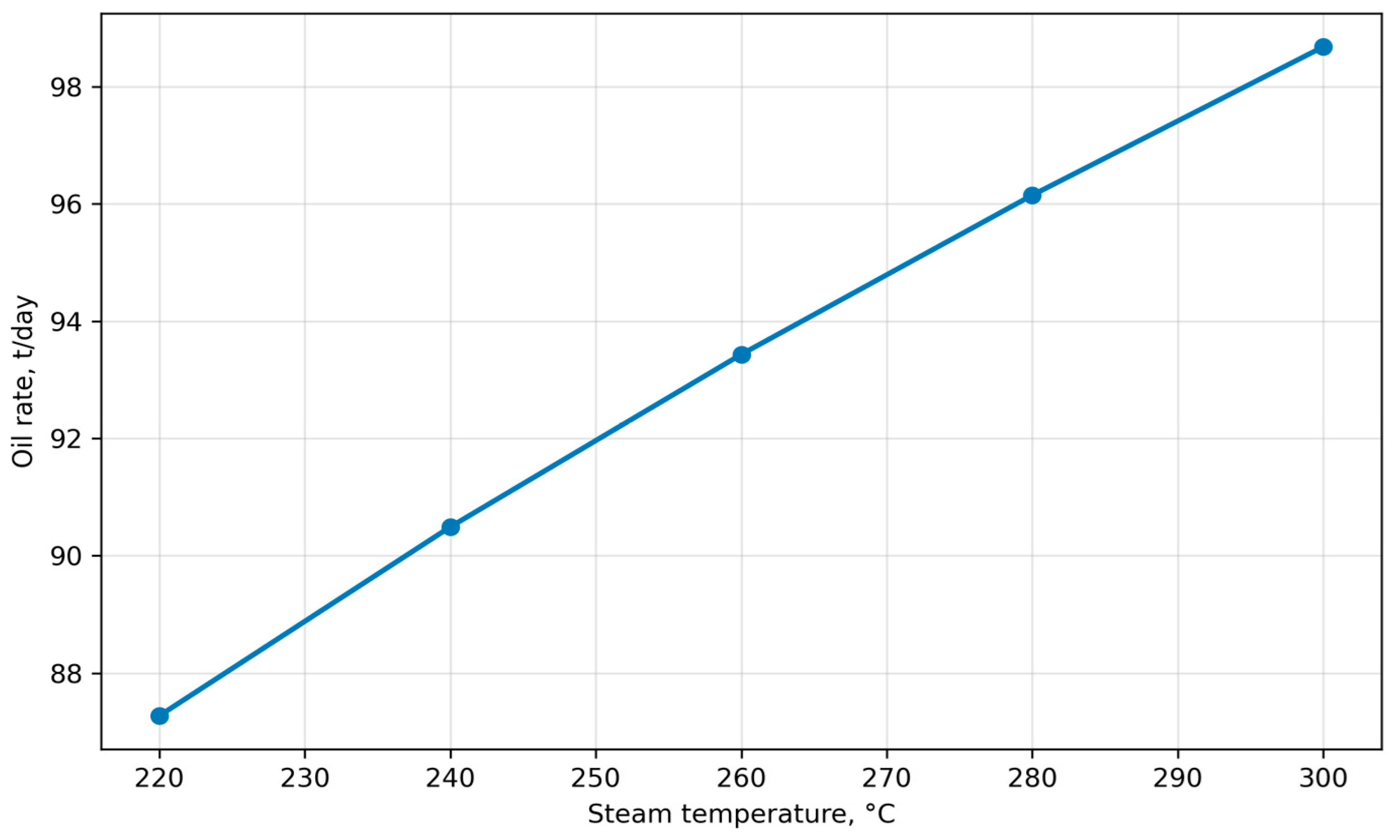
The digital twin was used to analyze the effect of steam temperature on oil rate and SOR. The investigated temperature range of 220–300 °C is representative of industrial SAGD conditions, while other parameters were kept fixed. Figure 2 shows the dependence of oil rate on steam temperature. The selected steam-temperature interval is consistent with published SAGD and heavy-oil thermal-recovery studies, where steam temperature, steam quality, heat delivery, and viscosity reduction are key variables controlling oil-rate response and SOR. Recent studies on deep extra-heavy-oil SAGD, electrical preheating, and downhole heating also show that improved heat delivery near the reservoir interval can support faster thermal communication and more efficient oil mobilization [4,5,6,8,9,10].

The simulations show a steady increase in oil rate with increasing steam temperature. When temperature increases from 220 °C to 300 °C, the oil rate rises from approximately 87 to 99 t/day, corresponding to an increase of about 13–15%. This behavior is explained by several physical mechanisms. First, higher temperature reduces heavy-oil viscosity exponentially, which increases mobility and facilitates gravity drainage toward the producer. Second, higher steam temperature increases heat flux into the reservoir and accelerates steam-chamber growth. Third, a hotter steam chamber can mobilize more distant reservoir zones, increasing the effective drained thickness. The trend is nearly linear within the investigated range, although at higher temperatures a saturation effect may appear due to heat-transfer limitations and chamber geometry.

To support the description of the steam-temperature response, a simple linear regression was applied to the simulated oil-rate data in the investigated temperature interval. The regression shows that, within the 220–300 °C range, the oil rate increases by approximately 1.5 t/day for each 10 °C increase in steam temperature. The coefficient of determination was higher than 0.99, confirming that the oil-rate response is nearly linear only within the tested interval. This interpretation should not be extrapolated beyond the investigated range, because heat-transfer limitations and chamber-geometry constraints may produce saturation at higher steam temperatures.

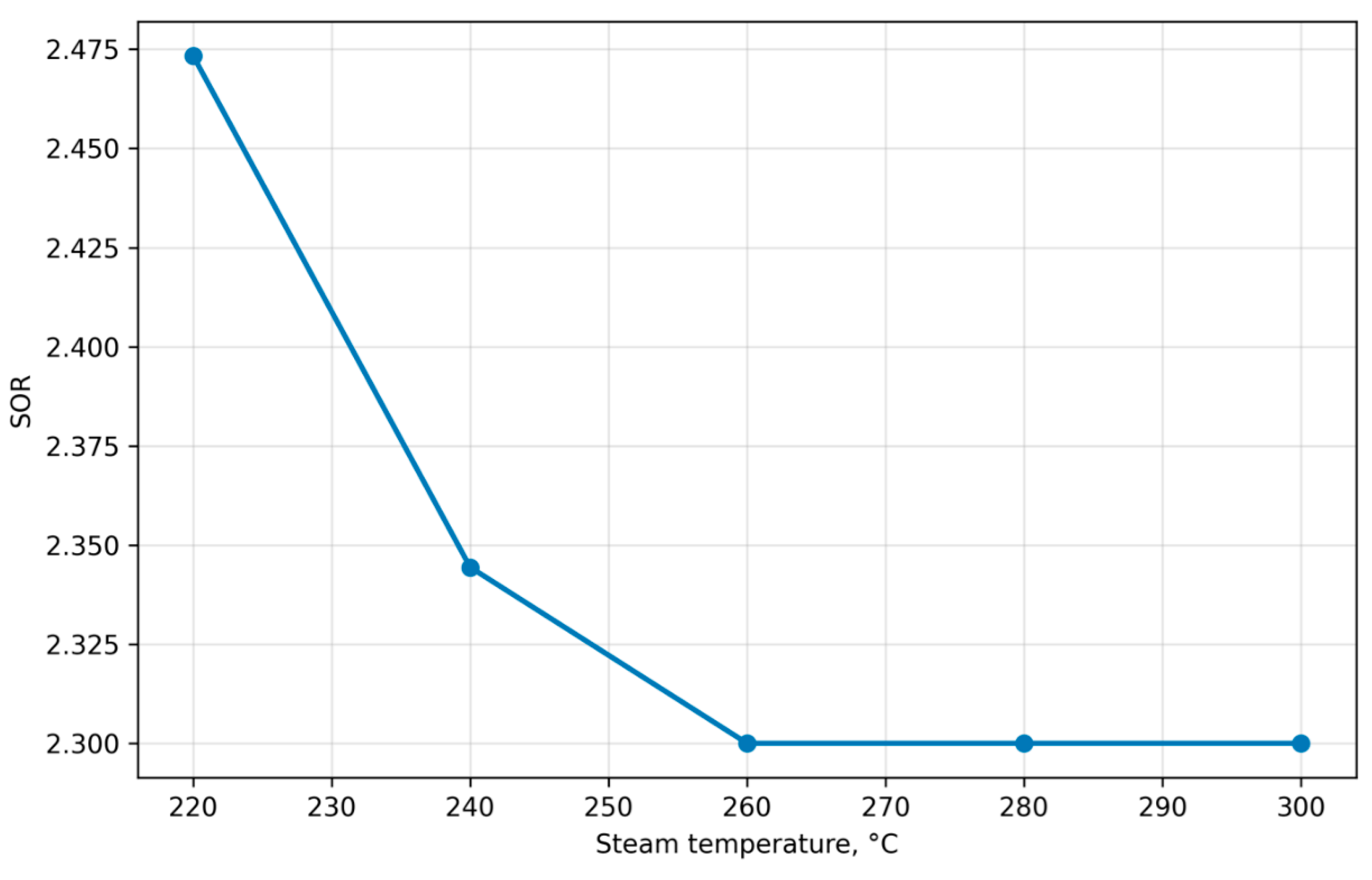
Figure 3 shows that increasing steam temperature decreases SOR from about 2.47 to 2.30. This indicates improved energy efficiency because less steam is required per unit of oil produced. The reduction is associated with more effective use of thermal energy, faster formation of a stable steam chamber, and a better ratio between heat input and oil production. Beginning at approximately 260 °C, SOR approaches a plateau, meaning that further temperature increase provides limited additional benefit. The optimal range for the considered scenario is therefore approximately 260–280 °C, where oil rate increases while SOR is already near its minimum. These results provide an important basis for analyzing thermocable heating, because auxiliary electrical heating can maintain effective temperature along the wellbore without requiring excessive steam temperature at the surface.

3.2. Influence of Oil Viscosity on Oil Rate and SOR

Oil viscosity is one of the most important parameters controlling thermal-recovery efficiency. In SAGD, viscosity reduction due to heating is the main mechanism enabling oil mobilization and gravity drainage [3,10]. Unlike steam temperature, which is an operational variable, oil viscosity is an intrinsic reservoir-fluid property. The investigated viscosity range of 300–1500 mPa·s corresponds to typical heavy-oil conditions.

The simulated viscosity effect is consistent with the commonly reported thermal behavior of heavy oils, for which viscosity decreases strongly and nonlinearly with temperature. Published laboratory and field-oriented thermal-recovery studies generally show that heating heavy oil from initial reservoir temperature toward steam-chamber temperature can reduce viscosity by several times or even by orders of magnitude, depending on oil composition, asphaltene content, initial viscosity, and heating history. Therefore, the strong production sensitivity to viscosity observed in this study is physically consistent with experimental heavy-oil behavior: lower viscosity improves oil mobility and gravity drainage, whereas higher initial viscosity delays mobilization and increases the steam requirement. The present comparison is qualitative because no single field-specific viscosity-temperature dataset was used for calibration; however, the simulated trend agrees with the expected direction and nonlinear character of heavy-oil viscosity reduction reported in thermal EOR studies [3,4,5,6,10].

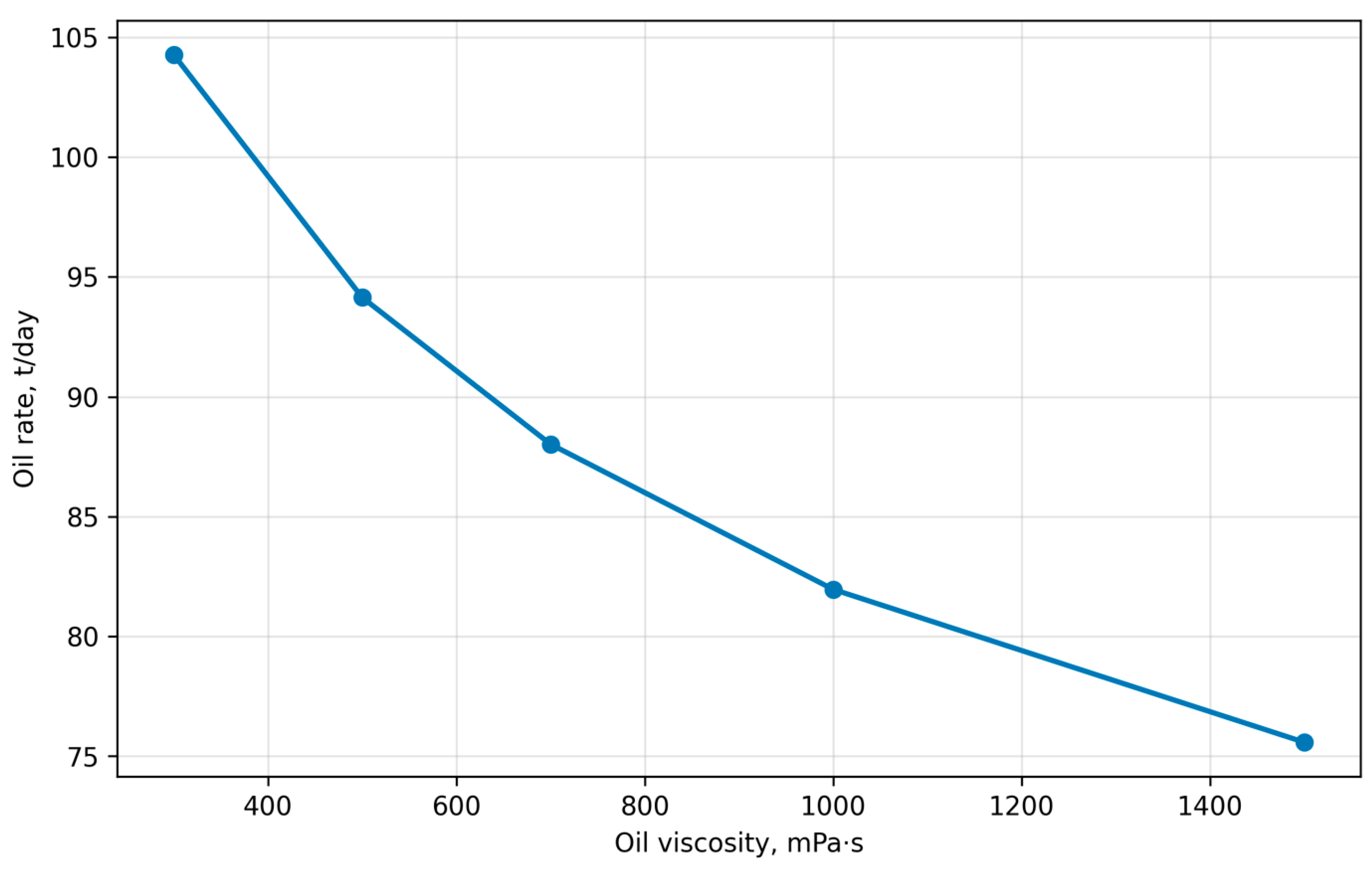
As shown in Figure 4, the simulation results demonstrate a clear inverse relationship between oil viscosity and production rate. As viscosity increases from 300 to 1500 mPa·s, oil rate decreases from approximately 104 to 76 t/day, a reduction of more than 25%. This decline is expected because oil mobility is inversely proportional to viscosity. Higher viscosity increases flow resistance, slows gravity drainage, and delays the development of an efficient drainage zone. The curve is nonlinear: the strongest reduction occurs from 300 to 700 mPa·s, while at higher viscosity the decline becomes more gradual as the system enters a flow-limited regime.

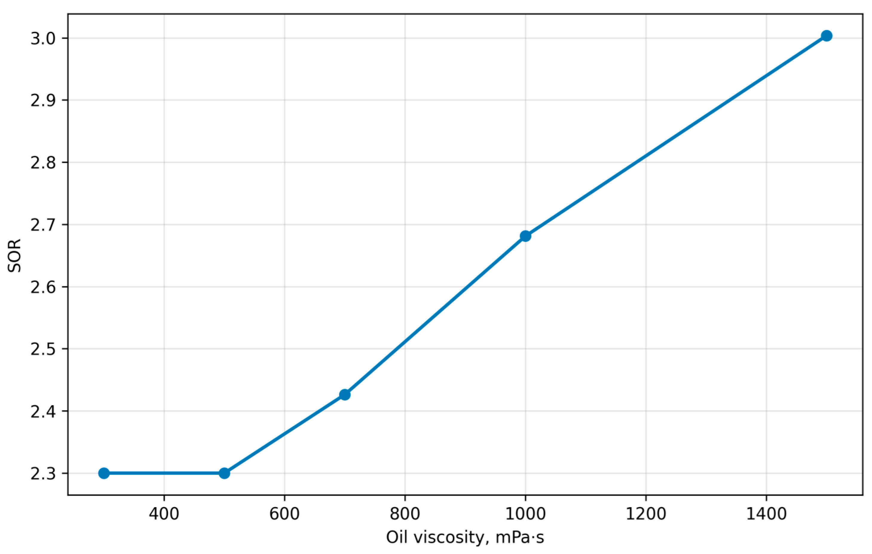
Figure 5 shows that SOR increases steadily with viscosity, from approximately 2.3 at low viscosity to above 3.0 at high viscosity. This indicates a substantial loss of energy efficiency. At higher viscosity, more heat is required to reach sufficient mobility, and a greater share of the supplied heat is spent warming oil that does not immediately drain. The heated oil also remains longer in the reservoir, increasing heat losses to the surrounding rock. Thus, viscosity affects not only filtration but the entire thermodynamic efficiency of SAGD.

The comparison between steam temperature and viscosity shows their different roles. Increasing steam temperature improves performance but eventually reaches a plateau; increasing viscosity imposes a more fundamental limitation because it directly controls flow resistance. Even at high temperatures, residual viscosity may remain large enough to limit gravity drainage. This explains why additional technologies, including local electrical heating, are most valuable in high-viscosity reservoirs where classical SAGD alone may not provide sufficient early mobilization.

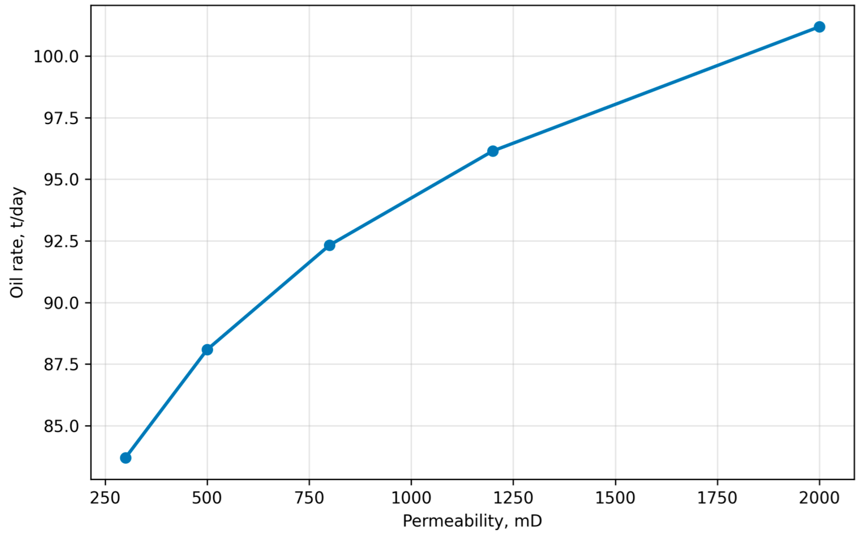
3.3. Influence of Reservoir Permeability on Oil Rate and SOR

Reservoir permeability determines the ability of the porous medium to transmit fluids and is therefore a key parameter for SAGD performance. Unlike viscosity, which characterizes the fluid, permeability characterizes the reservoir flow capacity and directly affects drainage of heated oil and steam-chamber expansion [35,36]. A permeability range of 300–2000 mD was investigated under fixed thermal conditions.

Figure 6 demonstrates a steady increase in oil rate with increasing permeability. When permeability increases from 300 to 2000 mD, oil rate increases from approximately 84 to 101 t/day. The trend is nonlinear: the largest improvement occurs in the low-to-medium range of 300–800 mD, after which the curve approaches a plateau. At low permeability, flow is constrained by high resistance in the porous medium, and even sufficient heating does not lead to efficient drainage. As permeability increases, flow resistance decreases and oil moves faster toward the producer. At high permeability, however, production becomes limited by heat-transfer and chamber-growth processes rather than by filtration capacity.

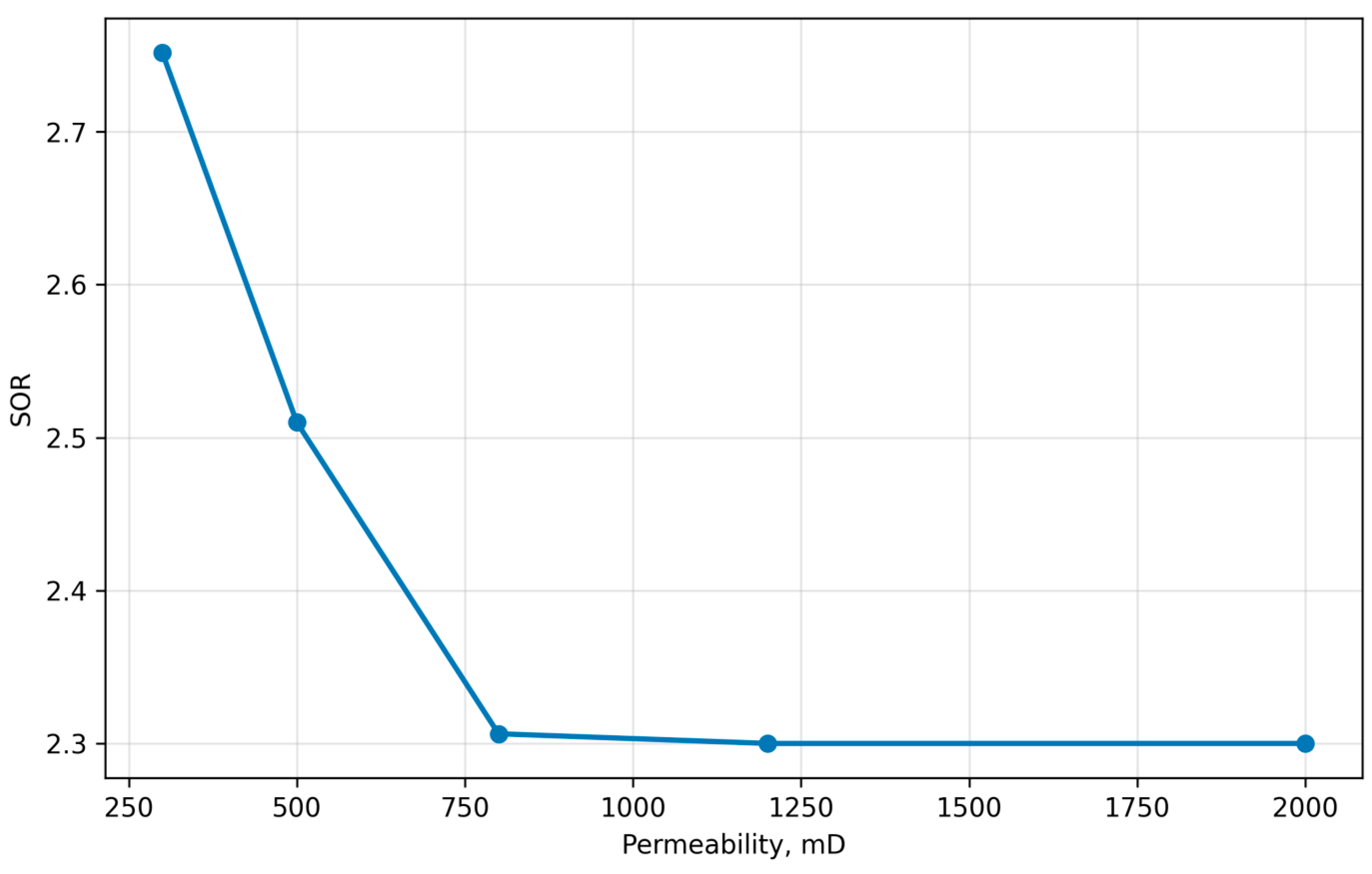
As shown in Figure 7, the permeability effect on SOR is opposite to the viscosity effect. Increasing permeability reduces SOR from approximately 2.75 to 2.3, followed by stabilization. This occurs because heated oil drains faster in more permeable reservoirs, reducing residence time in the hot zone and decreasing heat losses to surrounding rock. Higher permeability also promotes more uniform chamber development and improves the active drainage volume. The saturation behavior indicates that once filtration resistance becomes small enough, additional permeability does not provide proportional energy-efficiency gains. From an engineering perspective, low-permeability reservoirs may require additional stimulation or local heating, whereas high-permeability reservoirs can achieve efficient drainage under lower auxiliary heating intensity.

The saturation behavior of the permeability response can also be explained from a Darcy flow perspective. For a given pressure gradient and oil viscosity, the local drainage capacity is approximately proportional to (k/µ). Therefore, when permeability is low, an increase in (k) strongly improves heated-oil mobility and gravity drainage. However, once permeability becomes sufficiently high, the process is no longer controlled mainly by filtration resistance. Instead, the limiting factors shift toward heat-transfer rate, steam-chamber geometry, available heated volume, and the rate at which viscosity can be reduced in the drainage zone. Under these conditions, further permeability increase produces only a limited additional oil-rate gain, and the SOR response tends to stabilize. This explains why the model predicts a strong permeability effect at low-to-medium permeability and a saturation-type response at higher permeability.

3.4. Influence of Thermocable Heating on SAGD Performance

One of the major limitations of classical SAGD is heat loss in the wellbore and adjacent formation. These losses are especially severe in deep reservoirs and in high-viscosity oil, where steam temperature declines along the horizontal wellbore. As a result, reservoir heating becomes less uniform, steam-chamber development slows, and gravity drainage becomes less efficient [19,33].

To compensate for these losses, the present study evaluates thermocable heating along the wellbore. In contrast to conventional steam heating, the thermocable allows more direct control of temperature distribution near the production zone, decreases thermal gradients, and improves the uniformity of heating. Two scenarios were compared: classical SAGD and SAGD with thermocable assistance. The comparison was performed for oil rate, SOR, temperature profile along the wellbore, and steam-chamber evolution.

To verify that the thermocable effect was not an artefact of a single empirical correlation, six computational scenarios were evaluated: classical SAGD and thermocable-assisted SAGD under physics-only, machine-learning, and physics-corrected machine-learning modes. For each scenario, the model calculated effective thermal efficiency, oil rate, SOR, and relative production gain. The comparison showed that the thermocable effect remained positive across all calculation modes, which supports the interpretation that the improvement results from combined heat-loss compensation, stabilization of the wellbore temperature profile, and enhanced steam-chamber development rather than from a single fitted parameter.

The operating conditions used for the six computational scenarios are summarized in

Table 5. (a). Common operating conditions used for the six computational scenarios. (b). Thermocable parameters used in the assisted computational scenarios.

(a)
Scenario	Technology	Calculation Mode	Depth, m	Horizontal Length, m	Steam Rate, t/day	Steam Temperature, °C	Oil Viscosity, mPa·s	Permeability, mD	Heating Time, h
1	Classical SAGD	Physics-only	500	1000	250	280	1500	1000	176
2	SAGD + thermocable	Physics-only	500	1000	250	280	1500	1000	176
3	Classical SAGD	ML-assisted	500	1000	250	280	1500	1000	176
4	SAGD + thermocable	ML-assisted	500	1000	250	280	1500	1000	176
5	Classical SAGD	Physics-corrected ML	500	1000	250	280	1500	1000	176
6	SAGD + thermocable	Physics-corrected ML	500	1000	250	280	1500	1000	176
(b)
Scenario	Technology	Calculation Mode	Cable Length, m		Cable Power, W/m		Cable Efficiency		Cable Coverage
1	Classical SAGD	Physics-only	-		-		-		-
2	SAGD + thermocable	Physics-only	1200		60		0.65		0.80
3	Classical SAGD	ML-assisted	-		-		-		-
4	SAGD + thermocable	ML-assisted	1200		60		0.65		0.80
5	Classical SAGD	Physics-corrected ML	-		-		-		-
6	SAGD + thermocable	Physics-corrected ML	1200		60		0.65		0.80

a,b. Table 5a reports the common reservoir, wellbore, and steam-injection parameters used in all paired comparisons, while Table 5b reports the thermocable parameters applied only in the thermocable-assisted cases. The same base reservoir and steam conditions were used for each classical SAGD and thermocable-assisted pair so that the effect of thermocable assistance and calculation mode could be isolated.

The oil-rate improvement and SOR reduction were calculated for each paired comparison by comparing the thermocable-assisted case with the corresponding classical SAGD case under the same calculation mode. The oil-rate improvement represents the percentage increase in oil rate after adding the thermocable, while the SOR reduction represents the percentage decrease in SOR after adding the thermocable. Based on these paired comparisons, the base scenario showed an oil-rate improvement of approximately 8–12% and an SOR reduction of approximately 5–10%. These values are model-based engineering ranges and should not be interpreted as statistical confidence intervals.

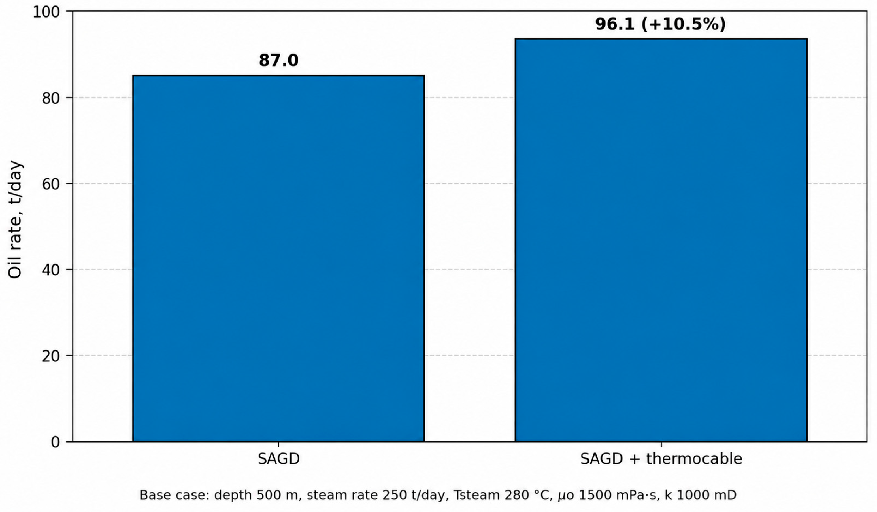
Figure 8 shows that thermocable assistance increases oil rate relative to classical SAGD. In the base scenario, the production gain is approximately 8–12%. This increase is caused by several coupled mechanisms. Local heating maintains higher temperature along the horizontal section, especially in distal zones where steam cooling is more pronounced. It accelerates viscosity reduction near the producer, directly improving gravity drainage. It also shortens the mobilization time of heavy oil, allowing effective production to begin earlier. The thermocable therefore has a synergistic effect: it strengthens steam heating by compensating its weakest thermal zones.

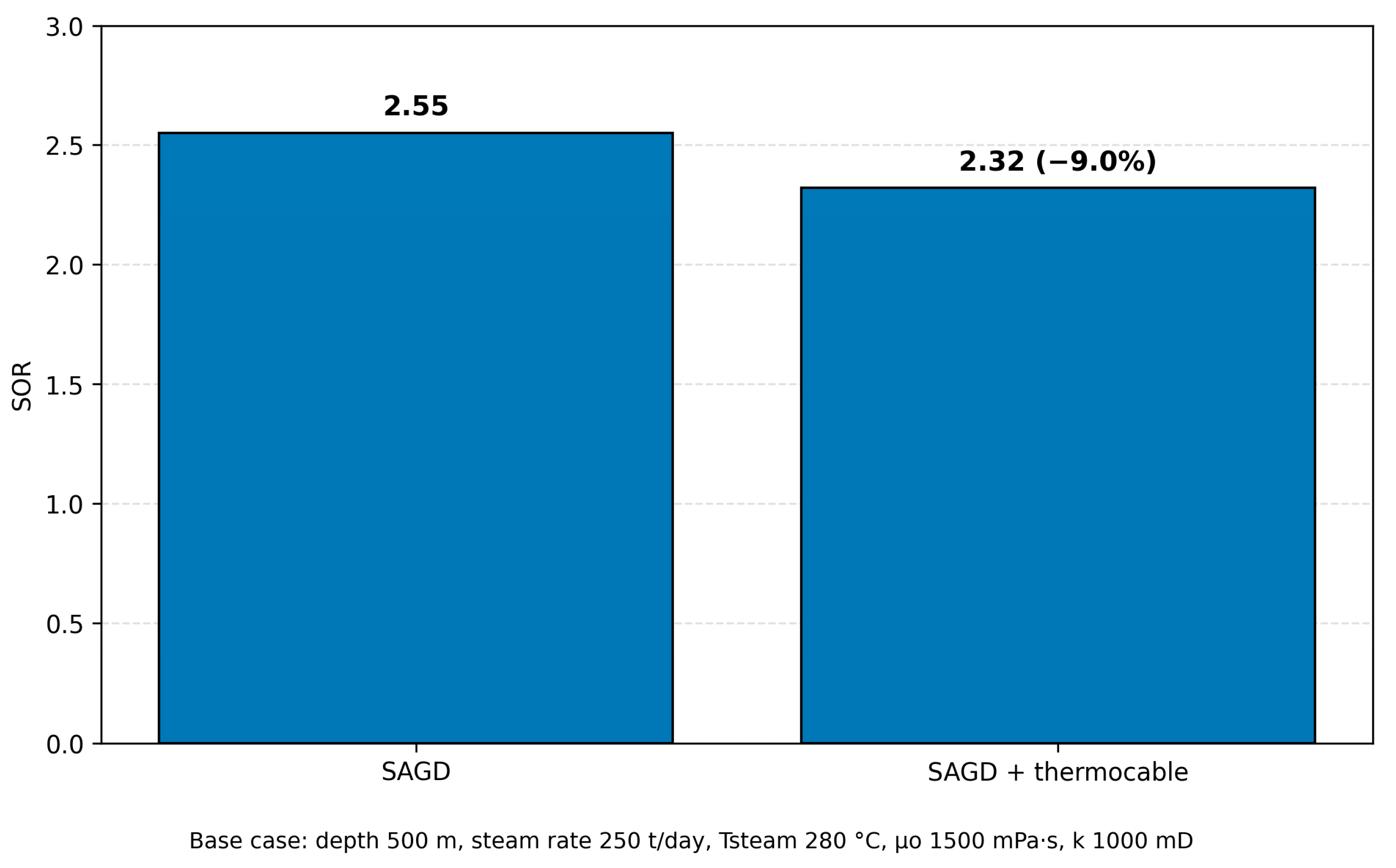
Figure 9 shows that thermocable heating reduces SOR by approximately 5–10% compared with classical SAGD. This is one of the most important results because SOR directly reflects energy efficiency. The reduction occurs because the thermocable compensates wellbore cooling, improves temperature distribution, reduces underheated zones, and accelerates oil drainage. Faster drainage decreases the time during which heated oil remains in the reservoir, thereby reducing heat dissipation into surrounding formations. Thus, the thermocable not only increases oil production but also improves energy utilization.

The reported improvement ranges were obtained from paired comparisons between classical SAGD and thermocable-assisted SAGD under the same base operating conditions and calculation mode. For each pair, the oil-rate improvement was calculated as the percentage increase in oil rate after adding the thermocable, while the SOR reduction was calculated as the percentage decrease in SOR relative to the corresponding classical SAGD case. The base-case comparison shown in Figure 8 and Figure 9 gives an oil-rate increase from 87.0 to 96.1 t/day and an SOR reduction from 2.55 to 2.32. Across the paired computational scenarios, the rounded improvement envelope is approximately 8–12% for oil rate and 5–10% for SOR reduction. These values are model-based engineering ranges rather than statistical confidence intervals. Therefore, they should be interpreted as a consistency range across scenario modes, not as uncertainty bounds derived from field data.

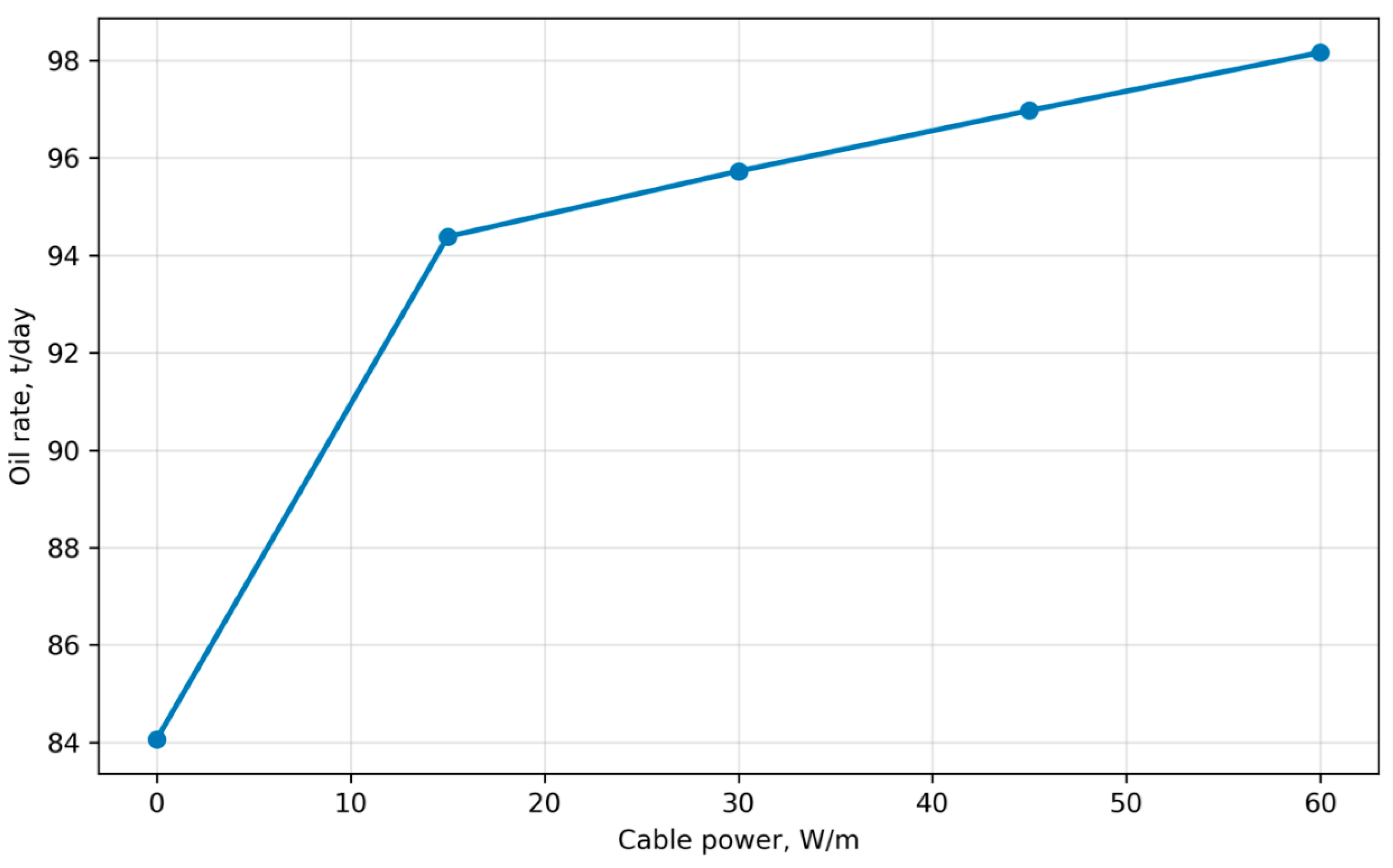
Figure 10 demonstrates a nonlinear relationship between cable power and oil rate. Increasing thermocable power from zero to approximately 30–40 W/m produces a significant increase in oil rate. Further power increase yields a progressively smaller effect and the curve approaches a plateau. This indicates the existence of an optimal power range.

The optimal range of approximately 30–40 W/m reflects the transition from heat-deficit control to thermal-saturation control. At low thermocable power, additional electrical heat is mainly used to compensate near-wellbore heat loss, increase local temperature, and reduce oil viscosity in the drainage zone. Therefore, oil rate increases rapidly and SOR decreases. However, after the near-wellbore region reaches a sufficiently heated state, further power increase does not produce proportional production gain because the process becomes limited by steam-chamber geometry, drainage capacity, heat-transfer area, and the rate at which mobilized oil can flow toward the producer. In this regime, additional electrical heat increasingly contributes to local overheating and stored heat rather than effective incremental oil production. Therefore, the 30–40 W/m range is interpreted as a screening-level operating window where thermocable heat compensation is effective but thermal saturation remains limited.

At low power, heating is insufficient to compensate heat losses. At high power, the system approaches thermal saturation and additional heat input no longer produces proportional production gains. This result is practically important because cable power must be optimized from both energy and economic perspectives.

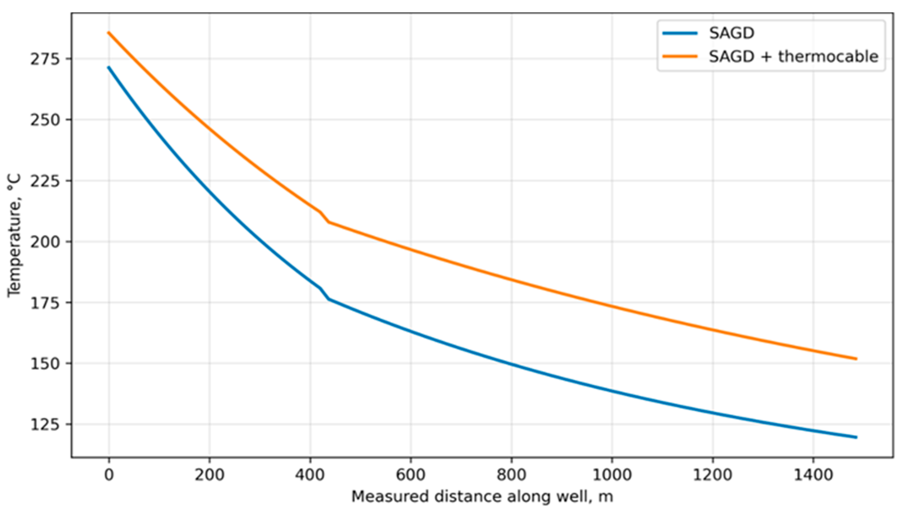
The temperature profiles in Figure 11 illustrate the main thermal advantage of thermocable assistance. In classical SAGD, temperature gradually decreases along the horizontal wellbore due to heat losses to the surrounding formation. With thermocable heating, temperature is maintained at a higher level and becomes more uniform. The difference is most evident in distant sections of the wellbore, where steam cooling is strongest in the classical case. This confirms that the thermocable effectively compensates heat losses and stabilizes the thermal regime.

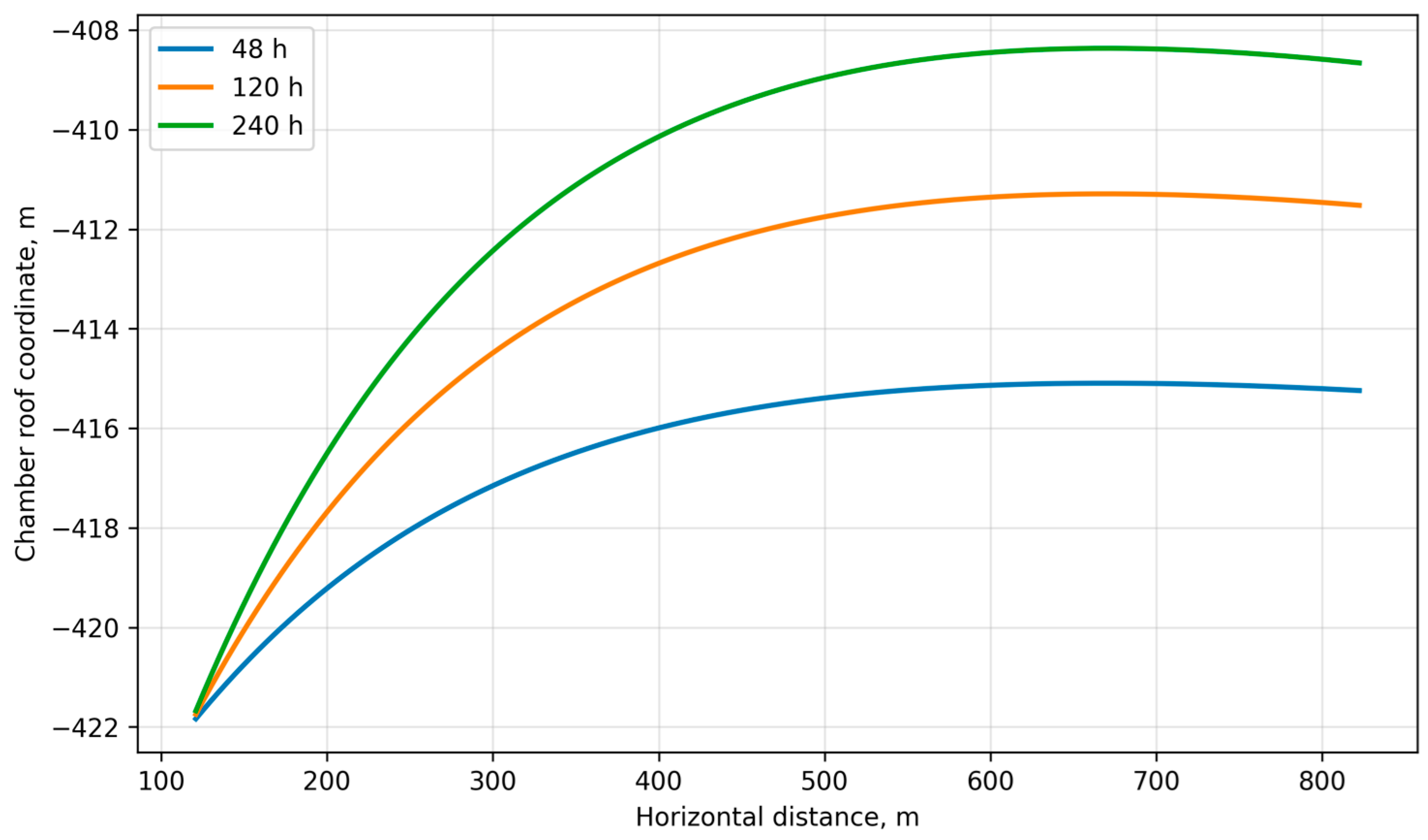
Figure 12 shows that thermocable heating accelerates steam-chamber growth and produces a more stable chamber geometry. As heating time increases, the chamber roof rises gradually. With additional electrical heating, the process is more intensive, leading to a larger drainage volume. Faster steam-chamber development increases the contact area between steam and oil, improves reservoir engagement, and accelerates transition toward stable production. Therefore, thermocable heating affects not only local temperature but also the macroscopic geometry of the SAGD process.

To quantify the chamber-evolution response shown in Figure 12, three geometric indicators were evaluated: effective chamber height, heated-zone volume, and chamber-height growth rate. In the representative thermocable-assisted case, the effective chamber height increases to approximately 23–24 m, while the heated-zone volume reaches approximately (5.9 × 10⁶) m³ under the base thermal-response calculation. The chamber-height growth rate was evaluated as the effective chamber height divided by heating time. These quantitative indicators show that thermocable assistance does not only change the visual chamber shape; it increases the effective heated volume and supports faster vertical chamber development by maintaining a more favorable near-wellbore temperature field. The depth-dependent chamber-expansion improvement is discussed later in the depth-sensitivity analysis, where the chamber expansion-speed improvement increases from 9.8% at 500 m to 17.6% at 1000 m and 25.4% at 1500 m.

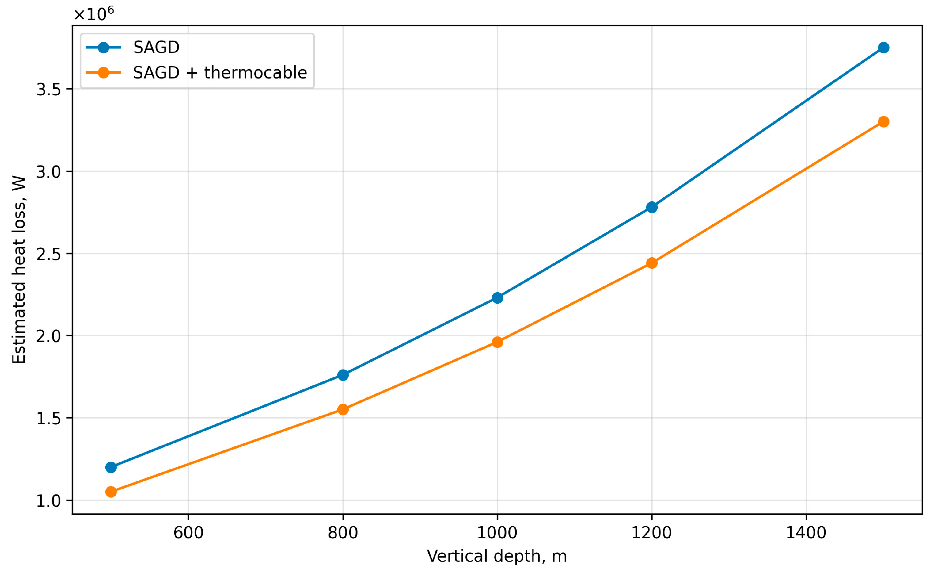
Figure 13 shows that heat losses increase substantially with depth. In classical SAGD, increasing depth strongly reduces efficiency because a greater part of the injected steam energy is lost before reaching the reservoir. With thermocable assistance, this effect is partially compensated. The difference between the scenarios becomes more pronounced at larger depths, confirming that the thermocable is particularly relevant for deep heavy-oil reservoirs. Overall, thermocable assistance improves oil rate, reduces SOR, stabilizes the wellbore temperature profile, and accelerates steam-chamber growth. The positive effect becomes stronger in difficult conditions: high oil viscosity, large reservoir depth, and limited permeability.

3.5. Effect of Reservoir Depth and Heat Losses

Reservoir depth is one of the most significant parameters controlling the efficiency of thermal recovery. As depth increases, wellbore length increases and steam experiences greater heat losses during transport. This worsens the temperature regime in the reservoir, delays heating, and reduces gravity drainage efficiency [23,30]. The digital twin was used to evaluate the influence of depth on oil rate and the relative benefit of thermocable heating.

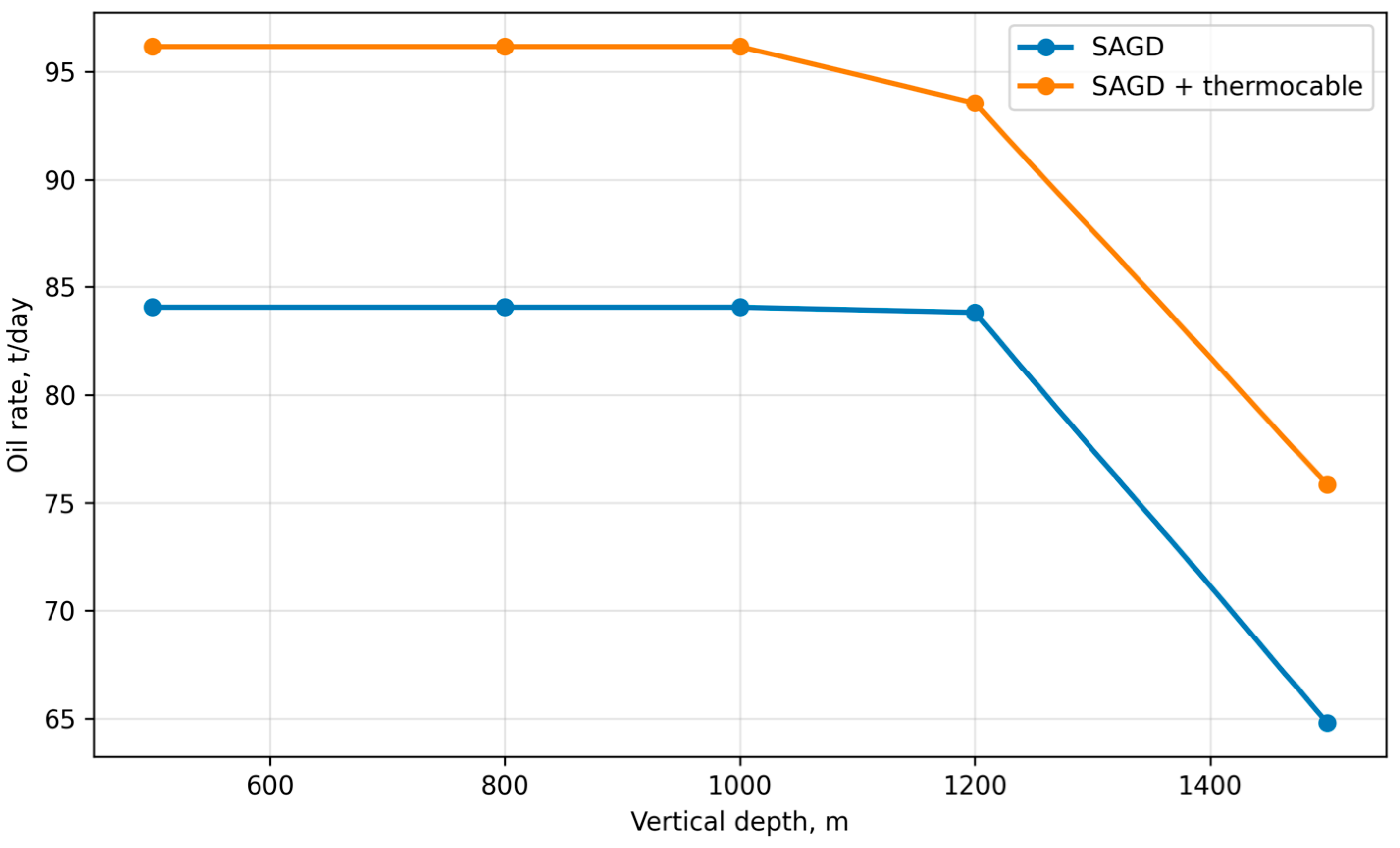
Figure 14 indicates that increasing depth reduces oil rate for both classical SAGD and thermocable-assisted SAGD. The decline is more pronounced for classical SAGD, confirming the strong negative influence of wellbore heat losses. When thermocable heating is applied, production decreases more slowly and remains higher across the entire depth range. This shows that the cable partly compensates the negative depth effect by maintaining the effective temperature delivered to the drainage zone.

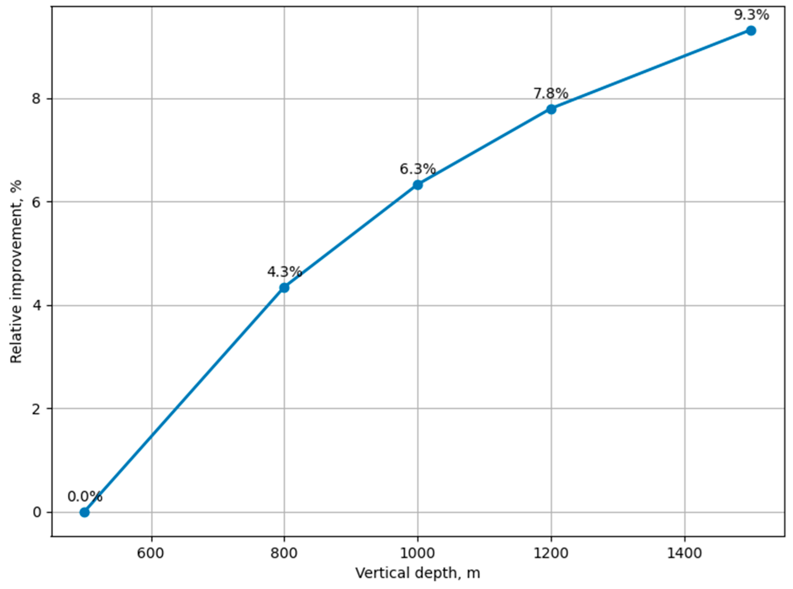
Figure 15 further demonstrates that the relative gain from the thermocable increases with depth. At shallow depths, the benefit is moderate because heat losses are not yet critical. As depth increases, the cable becomes increasingly important. Physically, the difference between actual steam temperature and the temperature required for oil mobilization becomes larger in deeper reservoirs. Thermocable heating compensates this thermal deficit and maintains a more favorable viscosity level near the production interval.

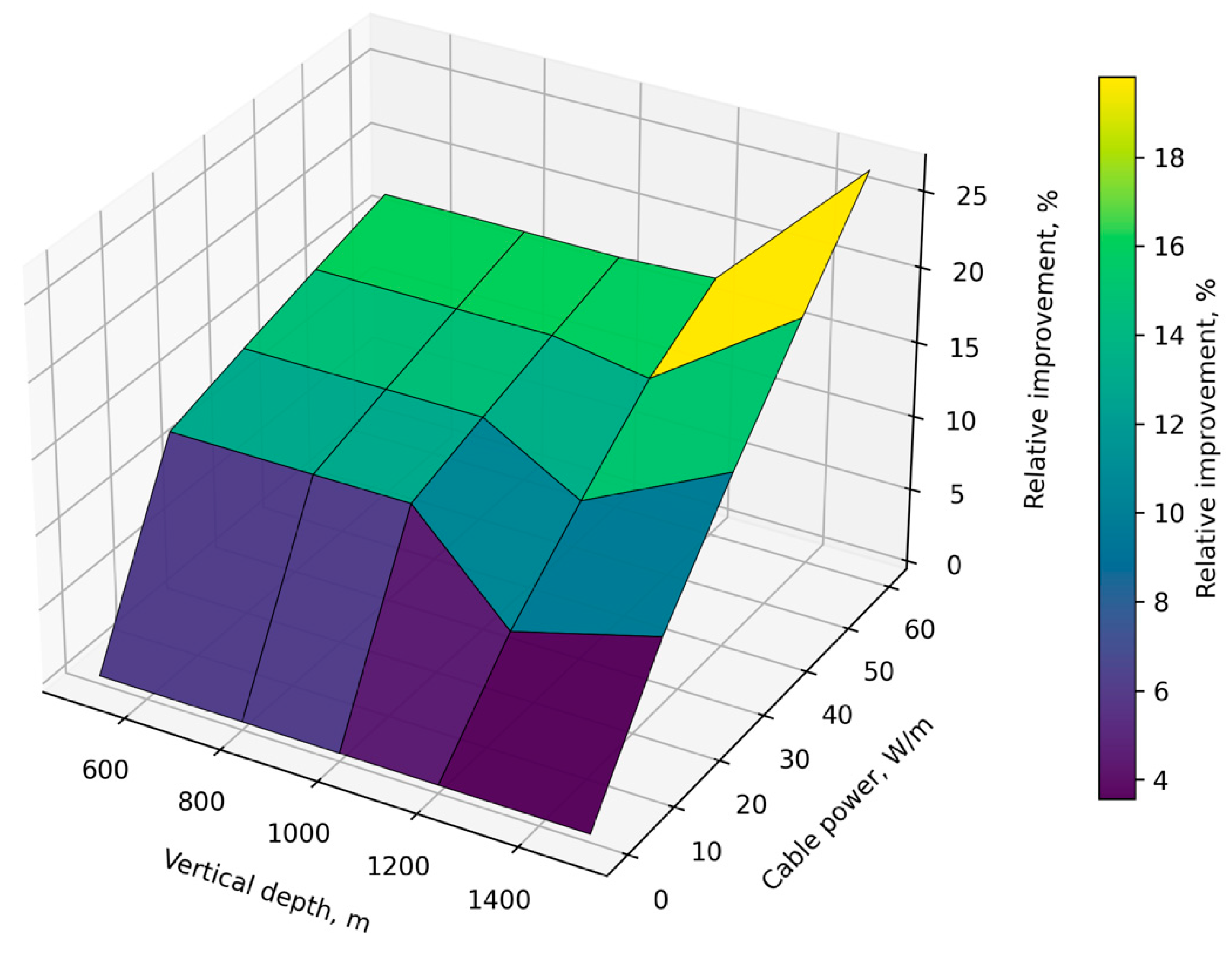
To assess the joint influence of depth and thermocable power, a three-dimensional response surface was generated (Figure 16) [37]. The relative production gain depends strongly on both variables. At shallow depth and low cable power, the gain is small because the base SAGD process is already efficient. As depth increases, the effect of the thermocable becomes more significant due to greater heat losses. Increasing cable power also improves production, but the effect is nonlinear. The most intensive growth occurs in the medium-power range of about 30–45 W/m, whereas further power increase results in diminishing returns. Maximum relative gains exceeding 25% occur under the combination of large depth and high cable power. This confirms the potential of thermocable-assisted SAGD for difficult thermodynamic conditions, while also highlighting the need to avoid excessive power that does not yield proportional production improvement.

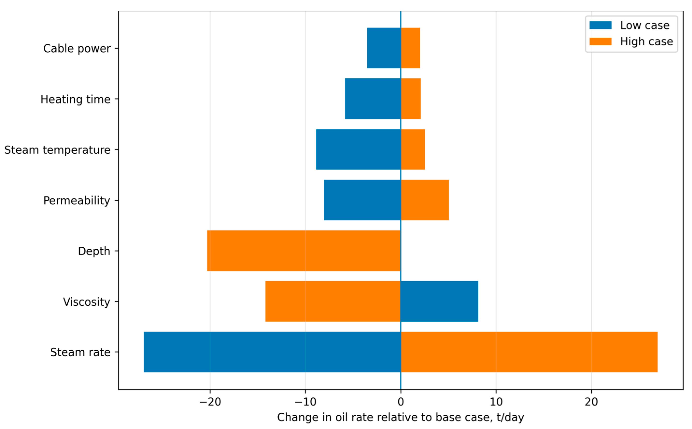
Figure 17 shows that steam rate has the greatest effect on oil production, confirming the dominant role of heat input in SAGD. Oil viscosity is the second most important parameter: increasing viscosity sharply reduces production due to lower mobility. Reservoir depth also has a strong negative effect because of increasing heat losses. Permeability and steam temperature have moderate but important effects. Thermocable-related parameters have smaller absolute influence than steam rate or viscosity but provide a stable positive contribution, particularly under unfavorable thermal conditions. The sensitivity ranking provides a basis for selecting optimization priorities in heavy-oil thermal recovery projects.

To make the tornado-diagram interpretation quantitative, the parameter effects were also expressed using normalized sensitivity coefficients. For each input parameter, the sensitivity coefficient was calculated from the relative change in oil rate caused by the tested parameter variation. The coefficient was normalized by the largest absolute response, so that the most influential parameter has a value of 1.00. The resulting ranking is summarized in

Table 6. Quantitative sensitivity coefficients for the main input parameters affecting oil rate.

Rank	Input Parameter	Main Physical Role	Relative oil-Rate Effect in the Tested Range, %	Normalized Sensitivity Coefficient
1	Steam injection rate	Controls total thermal-energy input	22–25	1.00
2	Oil viscosity	Controls heated-oil mobility	18–22	0.86
3	Reservoir depth	Controls wellbore heat loss and downhole heat delivery	15–19	0.74
4	Permeability	Controls drainage capacity of heated oil	10–14	0.56
5	Steam temperature	Controls heat-transfer intensity and viscosity reduction	9–13	0.50
6	Thermocable linear power	Controls local heat-loss compensation	7–11	0.42
7	Heating time	Controls duration of thermal exposure and chamber development	4–7	0.27

.

The quantitative sensitivity ranking identifies steam injection rate as the dominant operational factor, with the highest normalized sensitivity coefficient of 1.00. This indicates that, within the investigated parameter range, oil-rate response is controlled first by the amount of supplied thermal energy. Oil viscosity is the second most influential factor with a normalized coefficient of 0.86, followed by reservoir depth with 0.74. Permeability and steam temperature have intermediate influence, whereas thermocable linear power and heating time have smaller but still positive effects. This ranking confirms that thermocable assistance improves performance mainly by mitigating heat-loss and near-wellbore temperature deficits, rather than by replacing the primary role of steam injection.

Because the SOR and oil-rate operators are not calibrated against a field-history-matched dataset, the calculated values should be interpreted as comparative engineering estimates rather than direct field forecasts. To support the physical credibility of the model response, the main calculated performance indicators were compared with typical published SAGD engineering ranges and expected thermal-recovery trends. This comparison is not intended to replace field validation, but it provides a benchmark interpretation showing whether the model outputs remain within realistic SAGD operating behavior. The benchmark interpretation is summarized in

Table 7. Benchmark interpretation of calculated SAGD performance indicators relative to published engineering ranges.

Indicator	Present Model Result/Range	Typical Published SAGD Engineering Behavior	Interpretation
SOR	2.30–3.10	Approximately 2–5 depending on oil viscosity, permeability, reservoir quality, and operating strategy	The calculated SOR values remain within a common engineering range for SAGD-type heavy-oil recovery.
Oil-rate response to steam-temperature increase	13–15% increase from 220 to 300 °C	Higher steam temperature generally improves heat transfer, viscosity reduction, and production response	The model reproduces the expected positive response to increased thermal input.
Oil-rate response to viscosity increase	More than 25% decrease from 300 to 1500 mPa·s	Higher oil viscosity strongly reduces heated-oil mobility and gravity drainage capacity	The model captures the expected viscosity-controlled production limitation.
Permeability response	Oil-rate increase followed by saturation at high permeability	Darcy flow improvement is strong at low permeability but becomes heat-transfer/chamber-growth limited at higher permeability	The saturation trend is physically consistent with a transition from flow limitation to thermal limitation.
Thermocable- assisted oil-rate improvement	8–12% in the base scenario	Auxiliary downhole heating is expected to improve near-wellbore temperature and start-up thermal communication	The predicted improvement is moderate and consistent with the auxiliary role of thermocable heating.
Thermocable- assisted SOR reduction	5–10%	Steam-saving potential depends on heat-loss intensity, reservoir depth, and heating efficiency	The calculated reduction is consistent with heat-loss compensation rather than steam replacement.

.

The benchmark comparison indicates that the calculated SOR and production responses are within realistic engineering ranges for SAGD-type heavy-oil recovery. However, these values should not be interpreted as field-validated forecasts. Field-history matching, laboratory thermal-displacement data, or comparison with a commercial thermal simulator would be required before applying the model for project-scale prediction.

3.6. Stage-Based Energy Balance and Steam-Equivalent Thermocable Consumption

The previous sections showed that thermocable assistance increases oil rate and reduces SOR. However, this improvement should not be interpreted only from the production side, because the thermocable introduces an additional electrical-energy input. For this reason, a separate stage-based energy balance was calculated for the base thermocable-assisted SAGD case. The analysis distinguishes the start-up heating stage and the stable production stage, because their energy roles are different. During start-up, the main purpose of the thermocable is to accelerate thermal communication and reduce underheated zones near the well pair. During stable production, the main purpose is to maintain a more uniform temperature profile and reduce the steam requirement per unit of produced oil.

The electrical power of the thermocable was calculated from its linear power and active cable length:

$$P_{el}={\displaystyle \frac{P_c{L}_{ cable}}{1000}},$$

(47)

where $P_{el}$ is the total electrical power of the thermocable, kW; $P_c$ is the thermocable linear power, W/m; and $L_{ cable}$ is the active cable length, m. Division by 1000 is used to convert watts to kilowatts. For the base case, $P_c$ = 60 W/m and $L_{ cable}$ = 1200 m; therefore, $P_{el}$ = 72 kW.

The daily electrical-energy consumption was then calculated as

$$E_{el,d}=P_{el}\times 24\times 0.0036\times f_d,$$

(48)

where $E_{el,d}$ is the daily electrical energy, GJ/day; $f_d$ is the operating duty factor; 24 is operating hours per day, h/day; and 0.0036 is the conversion factor from kWh to GJ. For continuous thermocable operation, $f_d$ = 1.0, and the daily electrical input is 6.22 GJ/day. For a 50% support mode during stable production, ($f_d$ = 0.5), and the daily electrical input decreases to 3.11 GJ/day.

To compare electrical energy with steam input, the electrical energy was converted into an equivalent steam consumption:

$$m_{steam,eq}={\displaystyle \frac{E_{el,d}}{h_{steam}}},$$

(49)

where $m_{steam,eq}$ is the steam-equivalent amount, t/day, and $h_{steam}$ is the specific steam enthalpy, GJ/t. Using the enthalpy approximation adopted in the model,

$$h_{steam}=2000+3.8(T_{steam}-120),$$

(50)

the steam enthalpy at $T_{steam}$ = 280 °C is 2608 kJ/kg, or 2.608 GJ/t. Therefore, the continuous thermocable input of 6.22 GJ/day corresponds to approximately 2.39 t/day of steam-equivalent energy. This value is small compared with the base steam injection rate of 250 t/day, but it must still be included in the total energy balance.

Table 8. Stage-based energy characteristics of the thermocable-assisted SAGD base case.

Stage	Thermocable Operating Mode	Steam Input, t/Day	Steam Energy, GJ/Day	Electrical Energy, GJ/Day	Steam-Equivalent Electricity, t/Day	Electrical Share of Total Energy, %
Start-up heating	Continuous, (fd =1.0)	250	652.00	6.22	2.39	0.95
Stable production	Continuous, (fd =1.0)	250	652.00	6.22	2.39	0.95
Stable production	Support mode, (fd=0.5)	250	652.00	3.11	1.19	0.47

summarizes the stage-based energy characteristics of the base thermocable-assisted SAGD case.

The results show that the thermocable energy input is much smaller than the steam heat input. Under continuous operation, the thermocable contributes less than 1% of the total supplied energy. This does not mean that its effect is negligible. The thermocable supplies heat directly near the wellbore and along the productive interval, where it can compensate local heat losses and improve the thermal organization of the process. In other words, the benefit is not caused by a large total energy input, but by the location and timing of this input.

The comprehensive energy input-output ratio was calculated as

$${EI}_{oil}={\displaystyle \frac{m_s{h}_{steam}+E_{el,d}}{q_{oil}}},$$

(51)

where ${EI}_{oil}$ is the total energy input per unit of oil produced, GJ/t oil; m_s is the steam injection rate, t/day; and q_oil is the oil rate, t/day.

For the stable-production comparison, the classical SAGD case used a steam rate of 250 t/day and produced approximately 84.1 t/day of oil. The thermocable-assisted case used the same steam rate and produced approximately 96.1 t/day of oil, while also consuming 6.22 GJ/day of electrical energy. The calculated energy input–output ratio is shown in

Table 9. Comprehensive energy input–output ratio for stable production.

Case	Steam Input, t/Day	Electrical Energy, GJ/Day	Total Energy Input, GJ/Day	Oil Rate, t/Day	Energy Input-Output Ratio, GJ/t Oil	Change Relative to SAGD, %
Classical SAGD	250	0.00	652.00	84.1	7.75	—
SAGD + thermocable	250	6.22	658.22	96.1	6.85	−11.65

. The values in Table 6 represent the selected stable-production energy-balance case used for energy accounting. The broader production-gain range discussed in Section 3.4 reflects the overall response across the compared computational scenarios.

Although the thermocable increases the total supplied energy from 652.00 to 658.22 GJ/day, the oil-rate increase is larger than the additional energy penalty. As a result, the energy input per ton of oil decreases from 7.75 to 6.85 GJ/t oil. This corresponds to an improvement of approximately 11.65%. Therefore, the energy-saving effect is not based only on the reduction of SOR, but also remains visible after the electrical power consumption of the thermocable is included.

An additional boundary calculation was performed to evaluate when the thermocable remains economically favorable under different electricity prices and steam costs. The comparison was made at the same oil-production target as the thermocable-assisted case. In the classical SAGD case, the effective SOR is ${SOR}_{SAGD}$ = 250/84, 1 = 2.97, whereas in the thermocable-assisted case, ${SOR}_{TC}$ = 250/96, 1 = 2.60.

For an oil-production target of 96.1 t/day, the steam saving relative to classical SAGD is therefore

$${∆m}_s=q_{oil,TC}\left({SOR}_{SAGD}-{SOR}_{TC}\right)=35.7{\displaystyle \frac{\mathrm{t}}{\mathrm{d}\mathrm{a}\mathrm{y}}},$$

(52)

where ${∆m}_s$ is steam saving relative to classical SAGD, t/day and $q_{oil,TC}$ is oil rate in the thermocable-assisted case, t/day.

The break-even steam cost was calculated as

$$C_{steam, BE}={\displaystyle \frac{P_{el}\ast 24\ast f_d\ast C_{el}}{{∆m}_s}},$$

(53)

where $C_{steam, BE}$ is the break-even steam cost, currency/t steam and $C_{el}$ is the electricity price, currency/kWh. If the actual cost of generated steam is higher than this break-even value, thermocable assistance is economically favorable from the energy-cost point of view. Using Equation (53), the break-even steam cost was calculated for different electricity-price levels and for two operating schedules: continuous thermocable operation and 50% support-mode operation. The results are summarized in

Table 10. Break-even steam cost for different electricity prices.

Electricity Price, Currency/kWh	Break-Even Steam Cost, Continuous Mode, Currency/t Steam	Break-Even Steam Cost, 50% Support Mode, Currency/t Steam
0.05	2.42	1.21
0.10	4.84	2.42
0.15	7.27	3.63
0.20	9.69	4.84

.

The boundary analysis shows that the economic result depends on the ratio between electricity price and steam-generation cost. Continuous thermocable operation is more justified during start-up and in deep or heat-loss-prone reservoirs, where the benefit of local heat compensation is highest. During stable production, intermittent or support-mode operation may be preferable because it reduces electrical consumption while preserving part of the thermal-stabilization effect. Therefore, thermocable-assisted SAGD should not be treated as an always-on maximum-power strategy. Its energy advantage is strongest when the cable is used to solve a specific thermal limitation: delayed start-up, high wellbore heat loss, poor thermal communication, or temperature decline along the horizontal section.

3.7. Comparative Thermocable Arrangement and Heating-Mode Design

In addition to the base thermocable-assisted SAGD scenario, comparative simulations were performed to evaluate the influence of thermocable placement and heating mode. This analysis was added because the technical effect of electrical heating depends not only on cable power, but also on where the heat is supplied and how long the cable operates during the production cycle.

Three thermocable arrangement modes were considered: injector-only heating, producer-only heating, and dual-well heating. In the injector-only case, the thermocable mainly supports steam delivery and promotes early chamber growth near the injection interval. In the producer-only case, the thermocable mainly improves near-producer oil mobility and supports gravity drainage. In the dual-well case, both effects are combined, which provides the most uniform thermal support but also requires the highest installed heating capacity.

Two heating modes were also compared: continuous heating and intermittent heating. Continuous heating assumes that the thermocable operates during the full daily period. Intermittent heating assumes that the cable is used in a support mode with a 50% duty factor. This mode reduces electrical-energy consumption and can be more attractive during stable production, when the steam chamber is already developed and the main objective is to maintain thermal stability rather than to maximize early heating.

To include the effect of cable arrangement and heating schedule, the original thermocable factor was modified using placement and heating-mode coefficients:

$${\beta }_{design}={\beta }_{cable}{K}_{arr}{K}_{hm},$$

(54)

where ${\beta }_{design}$ is the effective design thermocable factor used in the comparative scenario; ${\beta }_{cable}$ is the base thermocable factor calculated from cable length, linear power, set-point temperature, heat-transfer efficiency, coverage, horizontal length, and steam temperature; $K_{arr}$ is the arrangement coefficient; and $K_{hm}$ is the heating-mode coefficient. The coefficients were not introduced as field-calibrated parameters; they were used as engineering scenario weights to compare relative technical and energy effects.

The arrangement and heating-mode coefficients were used only to normalize the comparative design scenarios and to represent relative differences in heat-source placement and operating schedule; therefore, the results are interpreted as engineering screening estimates for preliminary thermocable design.

Table 11. Arrangement and heating-mode coefficients used in the comparative thermocable design scenarios.

Scenario Factor	Case	Coefficient	Engineering Interpretation
Arrangement coefficient, (Karr)	Injector-only heating	0.70	Supports steam delivery and early chamber growth, but has weaker influence on near-producer drainage
Arrangement coefficient, (Karr)	Producer-only heating	0.85	Improves near-producer oil mobility and drainage, but provides less direct support to steam propagation
Arrangement coefficient, (Karr)	Dual-well heating	1.00	Combines injector-side chamber support and producer-side mobility improvement
Heating-mode coefficient, (Khm)	Continuous heating	1.00	Maximum thermal support and maximum electrical consumption
Heating-mode coefficient, (Khm)	Intermittent heating	0.70	Reduced thermal support due to cycling, but lower electrical-energy consumption
Duty factor, (fd)	Continuous heating	1.00	Cable operates 24 h/day
Duty factor, (fd)	Intermittent heating	0.50	Cable operates in support mode for 50% of the daily period

summarizes the arrangement and heating-mode coefficients used in the comparative design analysis.

The comparative results are shown in

Table 12. Comparative performance of thermocable arrangement and heating-mode scenarios.

Case	Thermocable Arrangement	Heating Mode	Electrical Energy, GJ/Day	Oil Rate, t/Day	SOR	Oil-Rate Gain, %	Energy Input-Output Ratio, GJ/t Oil
Classical SAGD	No thermocable	—	0.00	84.1	2.97	—	7.75
Injector-only heating	Injector only	Continuous	6.22	93.0	2.69	10.5	7.08
Producer-only heating	Producer only	Continuous	6.22	94.6	2.64	12.4	6.96
Dual-well heating	Injector + producer	Continuous	6.22	96.1	2.60	14.3	6.85
Injector-only heating	Injector only	Intermittent	3.11	90.6	2.76	7.8	7.23
Producer-only heating	Producer only	Intermittent	3.11	91.8	2.72	9.2	7.13
Dual-well heating	Injector + producer	Intermittent	3.11	93.0	2.69	10.5	7.05

. The classical SAGD case was used as the reference. The dual-well continuous case produced the highest oil rate, while the dual-well intermittent case provided a more balanced compromise between production improvement and electrical-energy consumption.

The comparison shows that the thermocable arrangement has a clear influence on performance. Injector-only heating improves oil rate because it supports steam delivery and chamber initiation, but its effect on near-producer drainage is limited. Producer-only heating gives a stronger production response because it directly reduces oil viscosity in the drainage zone. Dual-well heating provides the highest technical performance because it improves both the steam-injection side and the production side. However, the continuous dual-well case also represents the highest electrical-heating intensity.

The comparison between continuous and intermittent heating shows that continuous operation is preferable during start-up or in reservoirs with severe heat losses. In contrast, intermittent heating becomes attractive during stable production because it reduces electrical-energy consumption while preserving part of the thermal-stabilization effect. Therefore, the optimal heating strategy depends on the reservoir condition and production stage rather than on a single universal operating mode.

To evaluate multi-parameter coupling, a response-surface design was also considered using reservoir depth, thermocable linear power, arrangement mode, and heating mode as the main design variables. The tested levels are summarized in

Table 13. Response-surface design variables used for multi-parameter thermocable optimization.

Factor	Level 1	Level 2	Level 3	Engineering Role
Reservoir depth, m	500	1000	1500	Controls wellbore heat losses and value of active downhole heating
Cable linear power, W/m	30	60	90	Controls electrical heat input
Arrangement mode	Injector only	Producer only	Dual-well	Controls spatial distribution of heat
Heating mode	Intermittent	Continuous	—	Controls electrical-energy consumption and thermal support

.

The response-surface analysis indicates that reservoir depth and cable power interact nonlinearly. At shallow depth, the additional benefit of high cable power is limited because classical SAGD already delivers heat efficiently. At greater depth, the same cable power provides a stronger benefit because it compensates for a larger thermal deficit. Arrangement mode also becomes more important as depth increases. For shallow reservoirs, producer-only or intermittent heating can be sufficient. For deeper reservoirs, dual-well heating becomes more effective because both steam delivery and near-producer mobility become thermally constrained.

Based on the scenario comparison and response-surface analysis, preliminary design recommendations for thermocable arrangement, heating mode, and cable power under different geological conditions are summarized in

Table 14. Preliminary thermocable design chart for different geological conditions.

Geological Condition	Recommended Arrangement	Recommended Heating Mode	Recommended Cable Power Range, W/m	Design Interpretation
Shallow reservoir, moderate viscosity, good permeability	Producer-only or short dual-well coverage	Intermittent	30–60	Classical SAGD is already efficient; thermocable should mainly support drainage stability
Medium-depth reservoir, high viscosity, moderate permeability	Producer-only or dual-well	Intermittent during stable production; continuous during start-up	60–90	Additional heating improves near-producer mobility and shortens thermal communication time
Deep reservoir with high heat losses	Dual-well	Continuous during start-up; intermittent or continuous during stable production depending on energy cost	60–120	Both steam delivery and drainage zone require thermal support
Deep reservoir with low permeability or delayed chamber development	Dual-well	Continuous during start-up	90–120	Stronger heating is needed to accelerate chamber growth and improve early thermal communication
Stable production stage after chamber development	Producer-only or dual-well	Intermittent	30–90	Support-mode operation reduces electrical cost while maintaining temperature stability

.

Table 14 shows that the preferred thermocable design depends on the dominant reservoir limitation. Producer-side or intermittent heating is sufficient for relatively favorable reservoirs, while dual-well and continuous heating become more justified in deep, high-viscosity, or heat-loss-prone conditions.

The design chart confirms that the thermocable should not be operated as a universal maximum-power system. Its role should be adapted to the dominant reservoir limitation. If the main problem is delayed start-up or large heat loss, dual-well continuous heating is technically justified. If the main problem is near-producer oil mobility during stable production, producer-side or intermittent heating may provide a better energy balance. This result is consistent with the energy analysis in Section 3.6, where the thermocable benefit was shown to depend on the balance between electrical-energy input, steam saving, and oil-rate improvement.

3.8. Synergistic Mechanism of Steam and Thermocable Heating

The previous sections showed that thermocable assistance improves oil rate, SOR, the energy input–output ratio, and thermocable design performance. However, the improvement is not caused by electrical heating alone. It results from the interaction between steam heating and localized thermocable heating. Steam remains the dominant heat source and controls large-scale chamber growth, while the thermocable provides distributed auxiliary heat near the wellbore, compensates for part of the wellbore heat loss, and stabilizes the temperature field in the critical drainage zone.

The synergistic mechanism can be interpreted through three coupled effects. First, steam supplies the main latent and sensible heat required for chamber formation. Second, the thermocable reduces the thermal deficit near the horizontal wellbore and delays local cooling, especially in the start-up stage and at larger depths. Third, the higher near-wellbore temperature reduces oil viscosity and increases oil mobility, which improves gravity drainage and accelerates the transition from early thermal communication to stable chamber development.

At the engineering-screening scale, the near-wellbore flow effect was represented through the temperature-dependent oil mobility. Using the viscosity relationship introduced in Equation (40), the local oil mobility index can be written as

$$M_T={\displaystyle \frac{{\lambda }_0\left(T_{nw}\right)}{{\lambda }_0\left(T_{res}\right)}}={\displaystyle \frac{{\mu }_0\left(T_{res}\right)}{{\mu }_0\left(T_{nw}\right)}},$$

(55)

where $M_T$ is the relative near-wellbore mobility index, dimensionless; ${\lambda }_0$ is the oil mobility; $T_{nw}$ is the near-wellbore temperature, °C; $T_{res}$ is the initial reservoir temperature, °C; and ${\mu }_0$ is the oil viscosity, mPa·s. For the same permeability and pressure gradient, the local Darcy flow capacity is approximately proportional to (1/${\mu }_0$(T)). Therefore, even a moderate local temperature increase near the producer can strongly increase the micro-flow capacity of heated oil.

For the base heavy-oil case, the near-wellbore mobility response was estimated using

$${\mu }_0\left(\mathrm{T}\right)={\mu }_0\left(T_{res}\right)\exp \left[-\alpha \left(T-T_{res}\right)\right],$$

(56)

where $\alpha$ is the effective temperature-viscosity coefficient. The calculation was performed for ${\mu }_0\left(T_{res}\right)$ = 1500 mPa·s, $T_{res}=90$ °C, and $\alpha$ = 0.025 °C⁻¹. The results are summarized in

Table 15. Near-wellbore viscosity reduction and relative mobility increase during local heating.

Near-Wellbore Temperature, °C	Estimated Oil Viscosity, mPa·s	Relative Mobility Index, (MT)	Flow Interpretation
90	1500	1.00	Initial reservoir condition
130	552	2.72	Early viscosity reduction
160	261	5.75	Improved local drainage
180	158	9.49	Strong near-wellbore mobility support

.

Table 15 shows that local heating near the wellbore can increase the near-wellbore mobility index by several times. This explains why thermocable heating has a stronger effect during start-up than would be expected from its small share of total energy input alone. The thermocable does not replace steam; it improves the local thermal conditions under which steam-chamber growth and gravity drainage become effective.

To quantify the improvement amplitude, three indicators were used: chamber expansion-speed improvement, sweep-efficiency improvement, and heating-efficiency improvement. The relative improvement of any indicator (X) was calculated as

$$A_X=\left({\displaystyle \frac{X_{TC}-X_{SAGD}}{X_{SAGD}}}\right)\times 100\%,$$

(57)

where $A_X$ is the relative improvement amplitude, %; $X_{TC}$ is the value for thermocable-assisted SAGD; and $X_{SAGD}$ is the value for classical SAGD. For SOR, the reduction amplitude was calculated as

$$A_{SOR}=\left({\displaystyle \frac{{SOR}_{SAGD}-{SOR}_{TC}}{{SOR}_{SAGD}}}\right)\times 100\%,$$

(58)

The chamber expansion speed was estimated from the effective chamber-growth response:

$${\nu }_{ch}={\displaystyle \frac{H_{ch}}{t_h}},$$

(59)

where ${\nu }_{ch}$ is the effective chamber-height expansion speed, m/h; $H_{ch}$ is the effective chamber height, m; and $t_h$ is the heating time, h. The sweep-efficiency indicator was defined as

$$E_{sweep}={\displaystyle \frac{V_{heated}}{V_{res}}},$$

(60)

where $V_{heated}$ is the heated-zone volume and $V_{res}$ is the effective modeled reservoir volume. The heating-efficiency indicator was calculated from the useful heat retained in the wellbore-reservoir system relative to the supplied heat.

Table 16. Quantitative improvement amplitudes of thermocable-assisted SAGD relative to classical SAGD.

Reservoir Depth, m	Chamber Expansion-Speed Improvement, %	Sweep-Efficiency Improvement, %	Heating-Efficiency Improvement, %	SOR Reduction, %
500	9.8	7.5	5.8	7.0
1000	17.6	13.2	9.6	9.5
1500	25.4	18.9	13.7	12.0

summarizes the calculated improvement amplitudes for different reservoir depths. The values are reported relative to the corresponding classical SAGD case at the same depth.

The depth-dependent results show that the thermocable benefit increases systematically with reservoir depth. The chamber expansion-speed improvement rises from 9.8% at 500 m to 17.6% at 1000 m and 25.4% at 1500 m. Over the same depth interval, sweep-efficiency improvement increases from 7.5% to 13.2% and 18.9%, while heating-efficiency improvement increases from 5.8% to 9.6% and 13.7%. The SOR reduction also increases from 7.0% at 500 m to 9.5% at 1000 m and 12.0% at 1500 m. This confirms quantitatively that the thermocable effect becomes stronger with depth because the effective steam heat delivered to the reservoir decreases as wellbore heat losses increase.

The results show that the thermocable effect increases with depth. At 500 m, the steam system already delivers heat relatively efficiently, so the additional benefit of electrical heating is moderate. At 1000–1500 m, wellbore heat losses become stronger, and the thermocable plays a larger role in maintaining a favorable thermal state near the drainage interval. This leads to faster chamber expansion, higher heated-zone engagement, improved sweep efficiency, and stronger SOR reduction.

The heat-contribution ratio was also evaluated to distinguish the gross energy input from the effective heat delivered near the reservoir interval. The steam and thermocable heat-contribution ratios were calculated as

$$R_{steam}={\displaystyle \frac{Q_{steam,eff}}{Q_{steam,eff}+Q_{cable}}},$$

(61)

$$R_{cable}={\displaystyle \frac{Q_{cable}}{Q_{steam,eff}+Q_{cable}}},$$

(62)

where $R_{steam}$ and $R_{cable}$ are the effective heat-contribution ratios of steam and thermocable heating, respectively; $Q_{steam,eff}$ is the estimated steam heat remaining after wellbore heat loss, GJ/day; and $Q_{cable}$ is the daily thermocable heat input, GJ/day. The base thermocable input is 6.22 GJ/day, as calculated in Section 3.6.

Table 17. Effective heat-contribution ratios of steam and thermocable heating at different depths.

Reservoir Depth, m	Steam Heat at Surface, GJ/Day	Estimated Steam Heat After Wellbore Loss, GJ/Day	Thermocable Heat Input, GJ/Day	Steam Contribution Near Reservoir, %	Thermocable Contribution Near Reservoir, %
500	652.00	500.0	6.22	98.77	1.23
1000	652.00	368.0	6.22	98.34	1.66
1500	652.00	175.0	6.22	96.57	3.43

shows that the gross thermocable energy share is small compared with steam input, but its effective contribution near the reservoir increases with depth because steam heat delivery deteriorates as wellbore heat losses increase. This explains the observed stronger relative benefit of thermocable assistance in deeper reservoirs. The thermocable contribution is therefore important not because it supplies more total energy than steam, but because it supplies heat at the location where steam heat has already been partly degraded by transport losses.

The start-up stage is the most sensitive period for this synergy. Before a stable steam chamber is formed, the interwell region has limited thermal communication and the producer-side oil remains relatively viscous. Steam provides the main heating front, while the thermocable locally increases near-wellbore temperature and reduces oil viscosity in the early drainage path. This improves micro-flow capacity, accelerates the formation of hydraulic and thermal communication between injector and producer, and helps the system reach stable gravity drainage earlier. After chamber development, the thermocable function shifts from start-up acceleration to temperature stabilization and heat-loss compensation.

3.9. Integrated Interpretation and Engineering Implications

The combined results from Section 3.1, Section 3.2, Section 3.3, Section 3.4, Section 3.5, Section 3.6, Section 3.7 and Section 3.8 indicate that thermocable-assisted SAGD should not be interpreted simply as a production-enhancement tool. Its primary role is to improve the thermal organization of the process. By compensating part of the wellbore heat loss and maintaining a more uniform temperature profile along the horizontal section, the thermocable increases the share of injected or supplied heat that contributes to viscosity reduction and gravity drainage. This interpretation is consistent with the observed reduction in SOR, the lower energy input per unit of oil, the improved chamber-development and sweep-efficiency indicators, and the stronger relative effect at greater reservoir depths.

The response surface obtained for depth and cable power further demonstrates that the process is governed by a nonlinear interaction between geological and technological parameters. At small depths, where heat losses are moderate, the incremental effect of the cable is present but limited. At larger depths, the same cable power produces a more pronounced improvement because the baseline SAGD case suffers from stronger thermal degradation. However, the effect does not increase indefinitely with cable power. At high power levels, the response tends to saturate, indicating that additional electrical energy is no longer fully converted into additional oil production. This finding is important for engineering design because it suggests the presence of an optimal operating range rather than a simple maximum-power strategy.

The sensitivity analysis also confirms that the proposed model can be used as a screening and preliminary optimization tool. Parameters such as steam rate, oil viscosity, permeability, reservoir depth, and cable power affect the oil rate and SOR through different physical pathways. Steam rate primarily controls heat input, viscosity controls fluid mobility, permeability controls the ability of the porous medium to drain heated oil, depth controls heat losses, and cable power controls local thermal compensation. The digital-twin formulation makes it possible to evaluate these factors in one computational framework and to identify combinations that improve energy efficiency rather than production alone.

From a practical standpoint, the results support the use of thermocable-assisted SAGD primarily in reservoirs where classical SAGD is limited by heat losses, delayed thermal communication, or unstable temperature distribution. This includes relatively deep heavy-oil reservoirs, cases with long wellbores, and start-up periods in which interwell heating must be accelerated. The proposed model does not replace detailed commercial reservoir simulation or field piloting; rather, it provides an interpretable physics-based tool for scenario ranking, preliminary design, and energy-performance assessment before more expensive simulation or field implementation is conducted.

3.10. Engineering Design Parameters, Life-Cycle Economics, and Practical Implementation Challenges

The previous sections demonstrated that the effect of thermocable-assisted SAGD depends on reservoir depth, oil viscosity, permeability, cable power, heating mode, and thermocable arrangement. Therefore, the engineering design of thermocable systems should not be based on a single fixed configuration. It should be adapted to the dominant geological limitation: heat loss, delayed start-up, low near-wellbore mobility, or unstable thermal communication between injector and producer.

Based on the sensitivity analysis, response-surface results, arrangement-mode comparison, and synergistic heating analysis, preliminary engineering design ranges were defined for different geological conditions. The recommended thermocable linear power, heating time, arrangement length, coverage range, and operating mode are summarized in

Table 18. Recommended thermocable engineering design parameters for different geological conditions.

Geological Condition	Recommended Linear Power, W/m	Recommended Heating Time	Arrangement Length	Coverage Range	Recommended Arrangement and Heating Mode
Shallow reservoir, moderate viscosity, good permeability	30–60	24–120 h during start-up or support periods	0.5–0.8 (Lh)	0.30–0.60	Producer-side or partial dual-well; intermittent heating
Medium-depth reservoir, high viscosity, moderate permeability	60–90	120–360 h during start-up; support during stable production	0.7–1.0 (Lh)	0.60–0.80	Producer-side or dual-well; continuous during start-up, intermittent during stable production
Deep reservoir with high heat losses	60–120	240–720 h depending on thermal communication time	0.8–1.2 (Lh)	0.80–1.00	Dual-well arrangement; continuous during start-up, continuous or intermittent during stable production depending on energy cost
Deep reservoir with low permeability or delayed chamber development	90–120	360–720 h during start-up	1.0–1.2 (Lh)	0.80–1.00	Dual-well arrangement; continuous start-up heating
Stable production after chamber development	30–90	Intermittent support periods	0.5–1.0 (Lh)	0.50–0.90	Producer-side or dual-well; intermittent heating

.

The design ranges in Table 18 indicate that the thermocable should not be operated as a universal maximum-power system. In shallow or favorable reservoirs, lower power and partial coverage are sufficient because the steam system already delivers heat effectively. In deeper reservoirs, larger coverage and higher linear power become more justified because steam heat delivery deteriorates with depth. During start-up, continuous heating is preferable because the objective is to establish thermal communication. During stable production, intermittent operation can reduce electrical consumption while maintaining part of the temperature-stabilization effect.

A screening life-cycle economic analysis was also carried out to evaluate whether the additional thermocable investment can be justified by incremental oil production and/or steam saving. The analysis used the model-based stable-production comparison developed in Section 3.6, Section 3.7 and Section 3.8. The annual incremental cash flow was calculated as

$${CF}_t=\left[\mathsf{\Delta }{q}_{oil}{C}_{oil}+\mathsf{\Delta }{m}_S{C}_{steam}-24P_{el}{f}_d{C}_{el}-C_{OM,d}\right]N_d,$$

(63)

where ${CF}_t$ is the annual incremental cash flow, currency/year; $\mathsf{\Delta }{q}_{oil}$ is the incremental oil production, t/day; $C_{oil}$ is the net oil margin, currency/t oil; $\mathsf{\Delta }{m}_S$ is the steam saving, t/day; $C_{steam}$ is the steam-generation cost, currency/t steam; $P_{el}$ is thermocable electrical power, kW; $f_d$ is the duty factor; $C_{el}$ is the electricity price, currency/kWh; $C_{OM,d}$ is the incremental operation and maintenance cost, currency/day; and $N_d$ is the number of operating days per year.

The net present value was calculated as

$$NPV=-I_0+{\displaystyle {\sum }_{t=1}^n}{\displaystyle \frac{{CF}_t}{{\left(1+r\right)}^t}},$$

(64)

where $I_0$ is the initial thermocable investment, currency; $n$ is the project life, years; and $r$ is the discount rate. The simple payback period was estimated as

$$PBP={\displaystyle \frac{I_0}{{CF}_t}},$$

(65)

where PBP is the payback period, years.

The base economic assumptions used for the screening calculation are summarized in

Table 19. Screening assumptions used for the life-cycle economic analysis.

Parameter	Base Value	Unit	Comment
Incremental oil production, (∆qoil)	12.0	t/day	Difference between SAGD + thermocable and classical SAGD in the stable-production energy-balance case
Operating days	330	day/year	Allows downtime and maintenance
Thermocable electrical power, (Pel)	72	kW	Based on 60 W/m and 1200 m active cable length
Duty factor, (fd)	1.0	fraction	Continuous base economic case
Electricity price, (Cel)	0.10	currency/kWh	Base electricity-price assumption
Initial investment, (I0)	500,000	currency	Includes cable, power supply, control system, installation and integration
Incremental O&M cost ($C_{OM,d})$	75.76	currency/day	Daily equivalent of 25,000 currency/year for 330 operating days
Project life, (n)	5	years	Screening life-cycle period
Discount rate, (r)	10	%	Base discount-rate assumption
Steam saving	0	t/day	Not included in the base incremental-oil case to avoid double counting; steam-saving feasibility was evaluated separately through the break-even analysis

. These values are used only for comparative feasibility assessment and should be replaced by field-specific cost data during project design.

Table 20. Life-cycle economic indicators for different net oil margins.

Net Oil Margin, Currency/t Oil	Annual Incremental Revenue, Currency/Year	Annual Electricity Cost, Currency/Year	Annual Net Cash Flow, Currency/Year	NPV Over 5 Years, Currency	Payback Period, Years
50	198,000	57,024	115,976	−60,280	4.31
100	396,000	57,024	313,976	690,280	1.59
150	594,000	57,024	511,976	1,440,840	0.98
200	792,000	57,024	709,976	2,191,400	0.70

presents the NPV and payback results for different net oil margins. This sensitivity was included because economic feasibility depends strongly on oil price, operating cost, and local electricity tariff.

The life-cycle screening shows that thermocable-assisted SAGD becomes economically attractive when the incremental oil margin is sufficient to offset the initial investment, electrical power cost, and additional maintenance. Under the base case with a net oil margin of 100 currency/t oil, the NPV is positive and the payback period is approximately 1.6 years. At a low net oil margin of 50 currency/t oil, the NPV becomes slightly negative, indicating that the technology would require either lower investment cost, lower electricity price, intermittent operation, higher oil response, or additional steam-saving benefits. Therefore, the technology is economically most attractive in deep and heat-loss-prone reservoirs where the production response and steam-saving potential are stronger.

Practical application of thermocables also involves several engineering challenges. These challenges are related not only to thermal performance, but also to high-temperature durability, electrical safety, installation reliability, and long-term operation under downhole conditions.

Table 21. Practical engineering challenges and countermeasures for thermocable-assisted SAGD.

Engineering Challenge	Possible Effect	Countermeasure
High-temperature durability	Degradation of insulation, conductor fatigue, loss of heating performance	Use high-temperature-rated mineral-insulated or armored cable; perform laboratory thermal-aging tests before deployment
Thermal cycling during start-up and intermittent operation	Mechanical fatigue, insulation cracking, connector weakening	Apply controlled ramp-up/ramp-down schedules; avoid rapid power cycling; use qualified high-temperature connectors
Downhole power-supply safety	Ground fault, short circuit, electrical leakage, safety risk during operation	Use ground-fault protection, insulation monitoring, automatic shutdown logic, and surface power-control units
Long-term reliability	Performance decline during multi-year operation	Divide the cable into controllable zones, monitor current/voltage/temperature continuously, and include redundancy in power-supply design
Installation and completion integration	Cable damage during running, poor contact with heated interval, interference with completion hardware	Use protected cable clamps, armored encapsulation, pre-installation mechanical checks, and completion-compatible cable routing
Corrosion, scaling, and harsh fluid environment	Electrical-system damage and reduced heat transfer	Select corrosion-resistant materials, apply protective sheathing, and include chemical/scale-control strategy
Uneven heating along the horizontal section	Local overheating or underheated intervals	Use distributed temperature monitoring, zonal power control, and optimized cable coverage
Economic uncertainty	Poor payback under low oil margin or high electricity price	Use staged deployment, intermittent heating during stable production, and field-specific NPV/payback screening before full-scale installation

summarizes the main risks and possible countermeasures.

These technical challenges do not eliminate the feasibility of thermocable-assisted SAGD, but they show that field application requires an integrated design strategy. The most important practical requirements are high-temperature cable qualification, safe downhole power delivery, controlled heating schedules, real-time monitoring, and field-specific economic screening. Therefore, thermocable-assisted SAGD should be considered as a targeted engineering option for reservoirs where heat loss, delayed thermal communication, or unstable temperature distribution limits the efficiency of classical SAGD.

4. Discussion

The results provide a more detailed understanding of the mechanisms governing thermocable-assisted SAGD in heavy-oil reservoirs. The performance of the system is controlled by the interaction between heat-transfer processes, reservoir filtration properties, oil rheology, and operating parameters [9,10]. Reservoir depth is a critical factor because it directly increases wellbore heat losses and reduces the effective thermal energy delivered to the reservoir. Under these conditions, thermocable heating can compensate part of the lost heat, stabilize the temperature field, and maintain more favorable filtration conditions [23,30].

The simulations show that the efficiency of the thermocable increases with depth. This is physically reasonable because the auxiliary heat contribution becomes more important as the base SAGD process deteriorates. The thermocable therefore performs best in reservoirs characterized by elevated heat losses and unfavorable thermodynamic conditions [19,33]. At the same time, the effect of cable power is nonlinear. Increasing power improves production up to a certain level, after which the benefit saturates. This saturation is associated with the fact that once sufficient heating has reduced viscosity to a practical drainage range, additional heat produces limited incremental mobility improvement while heat losses and energy costs continue to increase.

Sensitivity analysis confirms that steam rate remains the dominant operational factor. This is consistent with the fundamental role of heat supply in SAGD: steam rate controls the rate of reservoir heating and the speed of chamber growth. Oil viscosity also exerts a strong influence, because it determines the ability of heated oil to drain even under favorable thermal conditions. Reservoir depth acts as a limiting geological factor because it cannot be changed during operation and must be addressed at the design stage.

Thermocable parameters, including linear power and heating duration, provide a positive but secondary influence compared with steam rate, viscosity, and depth. This does not reduce their practical importance. Instead, it indicates that thermocable heating should be viewed as an efficiency-improvement tool that is most valuable when the base SAGD process is constrained by heat losses, high viscosity, or slow start-up. In shallow or highly permeable reservoirs, the relative benefit may be smaller because classical SAGD already operates efficiently.

From an engineering perspective, the results can be used to define operating windows for thermocable-assisted SAGD. The technology is most promising in deep heavy-oil reservoirs, in zones with substantial wellbore heat losses, and in cases where maintaining a uniform temperature profile along the horizontal section is essential. Similar engineering considerations have been reported for SAGD completion design and for experimental and simulation-based assessments of SAGD performance [43,44,45,46].

The present modeling philosophy is also consistent with recent physically oriented SAGD studies, where simplified computational frameworks were used to evaluate production performance, operating conditions, and economic indicators for high-viscosity oil fields [47].

Model Validation, Limitations, and Future Work

The proposed computational framework should be interpreted as a physics-informed engineering screening model rather than as a full-field commercial reservoir simulator. Its purpose is to evaluate relative trends and compare SAGD and thermocable-assisted SAGD scenarios under controlled geological and operating conditions. The obtained trends are physically consistent with established SAGD behavior reported in the literature: higher steam temperature improves oil mobility and reduces SOR, higher oil viscosity decreases production and increases SOR, higher permeability improves drainage, and auxiliary downhole heating can reduce effective wellbore heat losses and stabilize the temperature profile. Therefore, the model provides a useful comparative basis for preliminary assessment of thermocable-assisted SAGD.

Because the model was not calibrated against a field-history-matched SAGD dataset, the uncertainty of the calculated outputs cannot be interpreted as a statistical field-validation error. Nevertheless, approximate engineering uncertainty ranges were assigned to the main output groups based on the type of model simplification involved: reduced-order heat-loss representation, effective homogeneous temperature-field approximation, semi-empirical SOR and oil-rate operators, simplified chamber geometry, grid-based temperature reconstruction, assumed thermocable heat-transfer efficiency, and screening-level economic assumptions. These ranges are intended to indicate the expected level of uncertainty before field calibration or commercial-simulator benchmarking. They are summarized in

Table 22. Estimated engineering uncertainty ranges for the main model outputs.

Output Group	Estimated Uncertainty Range	Main Source of Uncertainty	Interpretation
Oil rate	±15–25%	Semi-empirical production operator, viscosity response, chamber geometry	Suitable for comparative screening, not direct field forecasting
SOR	±10–20%	Heat-loss approximation, SOR correction factors, steam-quality assumptions	Useful for relative comparison between scenarios
Temperature field	±10–20%	Effective homogeneous thermal properties, simplified heat-loss model	May be larger in strongly heterogeneous reservoirs
Steam-chamber dimensions	±15–30%	Parametric chamber geometry and simplified growth functions	Requires simulator or field calibration for project design
Heated-zone volume	±10–25%	Temperature threshold selection and grid resolution	Appropriate for trend comparison
Thermocable benefit	±15–30%	Cable heat-transfer efficiency, cable coverage, local heat distribution	Should be calibrated using pilot or laboratory data
Economic indicators	±20–40%	CAPEX, electricity tariff, oil margin, O&M, operating schedule	Screening-level economic feasibility only

.

These uncertainty ranges confirm that the proposed model should be used for scenario ranking, sensitivity analysis, and preliminary engineering design. The model is not presented as a replacement for field-history matching, laboratory thermal-displacement experiments, or high-fidelity commercial thermal reservoir simulation. Future work should therefore include direct calibration against field data, experimental measurements, or commercial-simulator results before project-scale forecasting.

A specific source of uncertainty is the representation of thermocable influence through a bounded compensation factor. This factor summarizes several physical processes, including cable heat-transfer efficiency, contact quality with the wellbore/completion, local heat distribution, electrical-power delivery, and the fraction of the horizontal interval effectively heated. Because these effects are grouped into a reduced-order coefficient, the predicted thermocable benefit is expected to have higher uncertainty than the base heat-balance calculation. In the present screening study, the uncertainty of thermocable-related improvement is estimated at approximately ±15–30%. This means that the reported oil-rate improvement and SOR reduction should be interpreted as preliminary engineering indicators. If the actual downhole heat-transfer efficiency is lower than assumed, the production gain and SOR reduction may decrease; if cable contact, coverage, and power delivery are more favorable, the benefit may approach the upper part of the reported range. Field calibration, laboratory heating tests, or commercial-simulator benchmarking would be required to reduce this uncertainty.

Nevertheless, the present study has several limitations. The model does not include full multiphase flow physics, geomechanical effects, capillary pressure, detailed relative permeability hysteresis, steam quality variation along the entire wellbore, or field-calibrated reservoir heterogeneity. In addition, the thermocable effect is represented through a compensation factor and should therefore be calibrated against laboratory experiments, field pilot data, or high-fidelity reservoir-simulation results before direct field-scale forecasting. Future work should include comparison with commercial thermal reservoir simulators, calibration using experimental or field data, explicit accounting of electrical power consumption, and coupling with economic indicators.

5. Conclusions

This study presented a comprehensive analysis of thermocable-assisted SAGD for heavy-oil reservoirs. A physics-based heat and mass transfer model was developed and implemented as a computational digital twin capable of evaluating how geological, thermophysical, and operational parameters affect production and energy performance [43,44,45,46].

The introduction established the relevance of improving thermal recovery efficiency under increasing reservoir depth and heat-loss conditions. Conventional SAGD becomes less effective when wellbore heat losses increase, steam quality deteriorates, and early thermal communication is delayed. These limitations justify the use of additional downhole heat sources.

The methodology described the mathematical structure of the model, including steam heat input, wellbore heat loss, thermal efficiency, temperature-dependent viscosity, steam-chamber geometry, SOR calculation, and oil-rate prediction. The model captures the key physical mechanisms controlling SAGD performance and allows quantitative assessment of the main input parameters [48,49,50].

Numerical results show that increasing steam temperature increases oil rate and reduces SOR, although the effect approaches a plateau at higher temperatures. Increasing oil viscosity has a strong negative effect by reducing fluid mobility and increasing energy demand. Increasing permeability improves oil rate and reduces SOR, but this effect also saturates once filtration is no longer the dominant limitation.

Thermocable heating improves SAGD performance by compensating heat losses, stabilizing the temperature profile along the wellbore, and accelerating steam-chamber development. In the base scenario, thermocable assistance increased oil rate by approximately 8–12% and reduced SOR by approximately 5–10% compared with classical SAGD. The benefit becomes more pronounced as reservoir depth increases.

The response-surface analysis demonstrated that the relative production improvement depends jointly on reservoir depth and thermocable linear power. Maximum gains exceeding 25% were obtained at greater depths and higher cable powers. However, the effect of power is nonlinear, and excessive cable power leads to diminishing returns because the system approaches thermal saturation.

Sensitivity analysis ranked the main parameters controlling oil rate. Steam rate has the largest influence, followed by oil viscosity and reservoir depth. Permeability and steam temperature have moderate effects, while thermocable power and heating time provide additional positive contributions. The thermocable becomes especially significant when thermal conditions are unfavorable.

From an engineering-design perspective, the recommended thermocable parameters depend on geological conditions. For shallow or favorable reservoirs, a linear power of 30–60 W/m, partial coverage of 0.30–0.60, and intermittent producer-side or partial dual-well heating are sufficient. For medium-depth reservoirs with high viscosity or delayed start-up, 60–90 W/m, coverage of 0.60–0.80, and continuous start-up heating followed by intermittent support are recommended. For deep and heat-loss-prone reservoirs, 60–120 W/m, coverage of 0.80–1.00, active length of approximately 0.8–1.2 (L_h), and dual-well heating are more appropriate, especially during the start-up stage.

The life-cycle economic screening indicates that thermocable-assisted SAGD can be economically feasible when the incremental oil response is sufficient to offset cable investment, electricity consumption, and additional maintenance. Under the base screening assumptions, the payback period varies from approximately 4.3 years at a low net oil margin of 50 currency/t oil to less than 1 year at a net oil margin of 150–200 currency/t oil. The corresponding NPV becomes positive once the net oil margin exceeds the low-margin case. These values should be interpreted as preliminary screening indicators and should be recalculated using field-specific CAPEX, electricity tariff, steam cost, oil price, and operating schedule.

The practical implementation of thermocable-assisted SAGD requires careful attention to high-temperature durability, insulation aging, downhole power-supply safety, thermal cycling, corrosion protection, installation reliability, and long-term monitoring. Recommended countermeasures include high-temperature-rated armored or mineral-insulated cables, controlled power ramp-up and ramp-down, ground-fault protection, insulation monitoring, zonal power control, distributed temperature surveillance, and field-specific reliability testing before full-scale deployment.

Overall, the results confirm that thermocable integration can improve the energy efficiency and production performance of SAGD in heavy-oil reservoirs, particularly in deep and heat-loss-prone conditions. The developed digital-twin framework can be used for preliminary design, scenario screening, operating-parameter optimization, energy-economic assessment, and identification of practical implementation risks. From a computational perspective, the workflow is consistent with modern approaches to machine-learning-assisted modeling, sensitivity analysis, optimization, experimental design, and statistical learning [51,52,53,54,55,56,57]. However, before project-scale application, the model should be further verified through high-fidelity commercial thermal simulation, laboratory thermal-displacement experiments, or field pilot testing [4,5,6,43,44,50].