Article

Finite Element Analysis of Inflection Point Occurrence in Power Loss vs. Torque Curve of Permanent Magnet Synchronous Machines Towards Optimal Torque Distribution in Electric Vehicles

1
University of Zagreb, Faculty of Mechanical Engineering and Naval Architecture, 10002 Zagreb, Croatia
2
University of Zagreb, Faculty of Electrical Engineering and Computing, 10000 Zagreb, Croatia
*
Author to whom correspondence should be addressed.
Energies 2026, 19(13), 3040; https://doi.org/10.3390/en19133040
Submission received: 27 April 2026 / Revised: 16 June 2026 / Accepted: 23 June 2026 / Published: 27 June 2026

Abstract

The paper deals with a finite element analysis (FEA) of the occurrence of an inflection point in the power loss vs. torque curve of permanent magnet synchronous machines (PMSM), related to optimal torque distribution in multi-motor all-wheel drive electric vehicles. Simplified, analytical power-loss models of the electric motor suggest that the power loss curve is convex, and consequently, the equal front/rear torque distribution is optimal. On the contrary, experimental studies usually point to a non-convex power loss curve containing an inflection point, which leads to more complex torque distribution laws. With the aim of explaining the experimentally observed effects, a first-principle, FEA approach is applied to PMSMs of different types (interior vs. surface permanent magnets, IPM vs. SPM) and different vector control strategies (maximum torque per ampere vs. maximum efficiency). Additionally, the impact of vehicle transmission losses on the power loss curve inflection point occurrence is analyzed. The results demonstrate that in the IPM motors, the inflection point occurs more readily than in the SPM motors due to the greater reluctance torque capabilities, which can strongly saturate the q-axis even under flux-weakening conditions, thus creating a highly nonlinear iron loss torque dependency. Also, the rising transmission efficiency vs. torque curve contributes to the occurrence of an inflection point.

1. Introduction

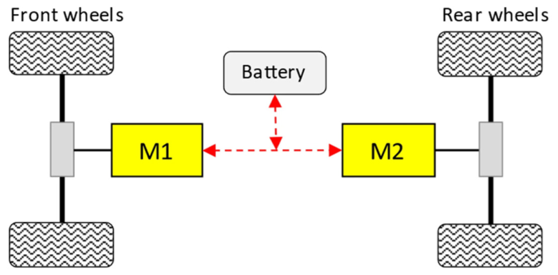
Rising environmental concerns have led to substantial efforts in electrifying road transport recently. Electric vehicles (EVs) stand out with over 20% of total sales globally in 2024 [1]. Nevertheless, the driving range on a single battery charge remains the primary drawback of electric vehicles. One way to increase the driving range [2] and, at the same time, contribute to the vehicle’s agility, stability, safety, and reliability [3], is to arrange the EV powertrain in a multiple-motor all-wheel drive (AWD) configuration (Figure 1). The multiple-motor propulsion is characterized by the actuator redundancy, which brings the opportunity of optimizing the torque distribution between motors to minimize the battery energy consumption, thus maximizing the driving range. Such torque distribution strategies typically bring savings in energy consumption by around 5% [4,5] when compared to equal (50:50) distribution. An additional 7% reduction in energy consumption can be achieved by incorporating the disconnect clutches placed between the electric motor gearbox and the driveline [6,7], because the disconnection eliminates the drag losses of inactive geared motors. A comprehensive review of recent developments in multi-motor EVs, including powertrain architectures, advanced control strategies, and specific technical challenges and solutions, is presented in [8].
There is usually a difference between the optimal torque distribution laws derived from analytical models of electric machine power losses and experimentally acquired power loss maps. In [10], employing an analytical model of copper losses I 2 R and similar iron losses I μ 2 R F e reduces the optimal front/rear-axle torque distribution in an EV with two equal permanent magnet synchronous machines (PMSM) to equal distribution (ED) across the entire operating range. A voltage-dependent second-order polynomial iron-loss model is used in [11] to maximize the total powertrain efficiency, resulting again in ED as the optimal solution. A d- and q-axis equivalent circuit physical machine model is employed in [12] to describe a surface-mounted permanent magnet (SPM) machine, where the iron losses are modeled through an equivalent iron-loss resistance. ED is again found to be optimal for equal motors, while for motors with different parameters, the optimal torque split ratio differs from ED but remains approximately constant across couple of low and high-speed operating points. In [13], a similar d- and q-axis equivalent circuit model is used for four-wheel identical SPM motors and augmented with a power inverter conducting and switching loss model and a mechanical loss model, resulting in ED to be optimal. In [14], d- and q-axis equivalent circuits are supplemented with hysteresis and eddy current iron losses modeled independently via two resistors, where hysteresis losses include frequency dependency. Employing the model to an EV with two different SPM motors results in a constant but unequal optimal torque split ratio determined by the motors’ asymmetry features. Furthermore, the equivalent circuit model is used in [15] for induction machines (IM), characterized by the ability to be demagnetized when not used to eliminate no-load losses. The torque distribution optimization results reveal that using a single-axle (SA) operation is optimal for low loads, while for higher torques, the AWD operation with ED is more efficient.
On the other hand, when the motor power loss model is based on experimentally acquired maps, the strategy combining SA and ED operation at low and high loads, respectively, is found to be optimal even in the PMSM-powered EVs with equal motors and no disconnect clutches, while the presence of a disconnected clutch leads to broadening the SA operating domain (see [5] and references therein). The vehicle velocity-dependent boundary demand torque curve, which separates the SA and ED modes, is usually called the switching torque curve. Multiple papers report the existence of switching torque across all vehicle speeds for dual interior PMSM-powered EVs based on experimentally recorded motor power loss maps. References [16,17] show that the switching torque is nearly constant in the motor constant torque region, and it reduces as the speed rises in the flux weakening region. On the other hand, reference [18] points out that the switching torque curve has lower values in the low-speed region and rises in the flux weakening region, while [19] reports that the switching torque (and thus the SA mode) exists only above a certain vehicle speed. The optimization results in [20] suggest that the switching torque exists across the full velocity range, but the exact shape of the switching torque curve is largely influenced by the transmission ratio. In [21], the boundary between the SA and ED modes is analyzed in the power rather than torque domain, and it is similarly found that SA and ED modes are optimal in low- and high-power regions, respectively. Two equal or different PMSMs with disconnect clutches are considered on each axle in [5] and [22], respectively, and the reported results indicate that the SA operation area broadens when disconnect clutches are added, and the AWD torque split ratio varies throughout the operating range.
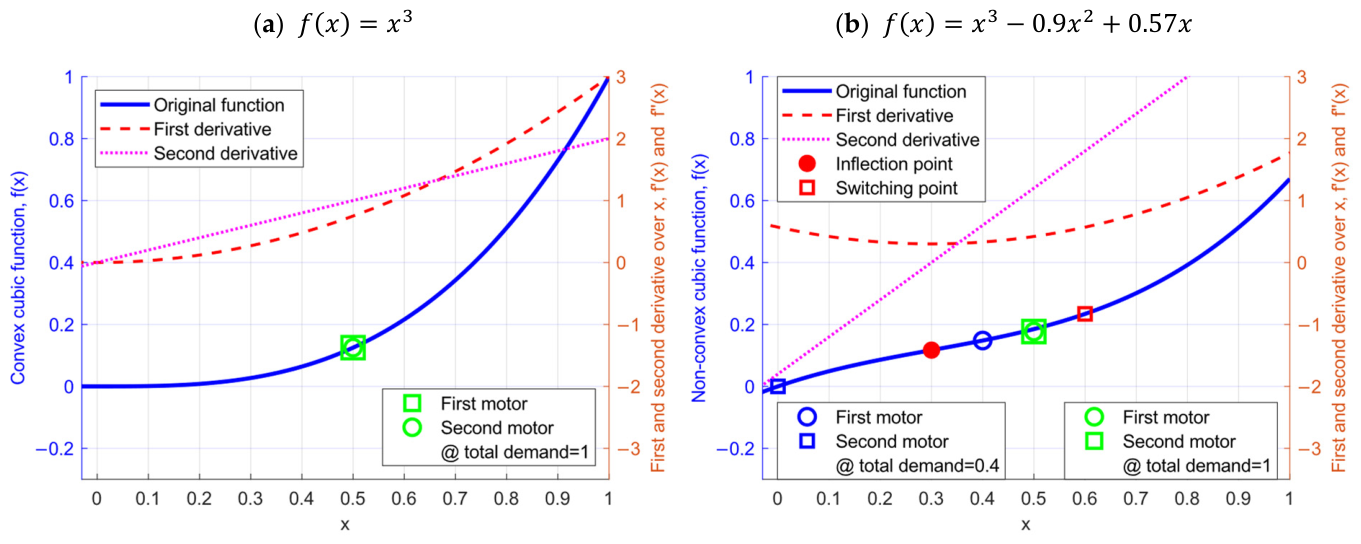
An analytical derivation of the switching torque is presented in [23,24] based on the third-order polynomial function describing the experimentally recorded machine power loss vs. torque curve. It is shown therein that the optimal SA-ED operation is a consequence of the power loss curve transition from concave to convex shape as the powertrain torque demand grows, i.e., it relates to the occurrence of an inflection point in the power loss vs. torque curve. In other words, the inflection point is defined as the point at which the second derivative of the power loss curve changes its sign, as illustrated in Figure 2b. On the other hand, for a purely convex curve (Figure 2a), the power loss increases progressively (exceeds a linear rate), thus making the second derivative strictly positive, so with no inflection point present. In this case, the ED point x 1 = x 2 = 0.5 designated in Figure 2a is optimal, since the total losses of the front and rear motors would be higher in any other pair of points having the total normalized demand of x = x 1 + x 2 = 1 , as a consequence of a progressively rising power loss curve. In contrast, when the power loss curve is concave in the low torque region, it is optimal to alternate the SA and ED modes (green and blue points in Figure 2b), respectively, depending on whether the torque demand is lower or higher than the switching torque (designated in Figure 2b by the red square based on the expression derived in [24]). Power loss measurements in [25,26] confirm that the power loss characteristic can be non-convex in low-load conditions, i.e., it is not strictly convex across the full torque range [27].
Although the occurrence of EV drive power loss vs. torque curve inflection point is experimentally evidenced in many papers (e.g., [22,23,24,25,26]) and employed in optimal torque distribution control strategies, it remains unclear what the exact reason for the inflection point effect is, and why the existing analytical physical models cannot predict the effect (but rather lead to a convex power loss curve). The potential root cause is related to the fact that the existing physical models rely on constant inductances in the d- and q-axis, thus omitting to describe the flux saturation present in high-performance EV machines. This hypothesis can be verified by using first-principles finite element analysis (FEA), which is not exploited in the available literature. To fill the gap, the PMSM is modeled in this paper in the Ansys MotorCAD FEA environment. Even though the FEA approach is time and computational resource-demanding, it is widely adopted as a high-fidelity method due to superior precision and universality [28]. To gain broader insights into the analyzed phenomena, the FEA concerns both surface (SPM) and interior permanent magnet (IPM) variants of synchronous machines, and both maximum torque per ampere (MTPA) and maximum efficiency (ME) current vector control strategies. In practice, IPM machines are widely used in electric vehicle propulsion systems due to their superior flux-weakening capabilities, which are essential for achieving the wide speed range required under realistic driving conditions. Consequently, the inflection-point analysis becomes particularly important for the IPM motor variant. It should be noted that IPM machine-related studies in [15,16,17] report the optimal SA/ED torque distribution based on the experimentally recorded power loss maps, suggesting the presence of an inflection point in the power-loss vs. torque curve.
The main contributions of the paper are summarized as: (i) development of PMSM FEA models capable of describing the experimentally observed machine power loss vs. torque curve inflection point for accurate design of optimal torque distribution strategies in multi-motor AWD EVs, and (ii) analysis of the root causes for the inflection point occurrence based on the FEA results.
The paper is structured in the following way: Section 2 describes the FEA approach, Section 3 presents SPM and IPM machine performance maps and describes MTPA and ME current vector control, Section 4 analyzes the inflection point occurrence, Section 5 presents and discusses the related optimal torque distribution results and influence of transmission losses and Section 6 summarizes the main conclusions.

2. Finite Element Modeling of Electric Motors

2.1. Motor Design

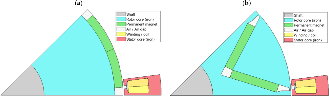
SPM and IPM synchronous motors having 48 slots and 8 poles (Figure 3) are modeled in Ansys MotorCAD 2024.1.3 for the purpose of comparative FEA. Table 1 gives the basic specifications of the motors [29]. The outer dimensions are equal for the two motors: outer diameter of 260 mm and axial length of 200 mm. The total masses of the active motor parts equal 51.8 kg and 51.5 kg for the SPM and IPM motors, respectively. The maximum current density of 30   A / m m 2 is typical for high-performance PMSMs, as commonly found in electric vehicle applications, to achieve the desired high torque and power output while maintaining the prescribed thermal limits [30,31]. The cooling system could be based on a water-jacket housing [31] and/or oil-spray cooling [32], and its design is beyond the scope of this paper.
The motor materials selected for modeling purposes are listed in Table 2. Pure copper and M530-65A iron are selected as the common winding and non-oriented electrical steel materials, respectively. N30UH material is selected as a typical representative of high-performance traction machines’ NdFeB permanent magnets characterized by high flux density and thermal stability.
For the sake of a fair comparison of the SPM and IPM motors, the stator parameters are also kept identical for both motor types, and they are listed in Table 3. Due to the fundamentally different rotor geometries (Figure 3), only the airgap length of 1   m m , the rotor diameter of 198   m m , and the magnet thickness of 6.7   m m are kept identical for the two motors (Table 4). The remaining rotor parameters are chosen by matching magnetic flux density saturation levels in both motors (see Section 2.2 for details). Although it may not be very representative from the standpoint of optimizing each individual motor, this approach allows a meaningful comparison of the motors’ power losses while accounting for their geometrical differences.

2.2. Rotor Parameter Selection Approach

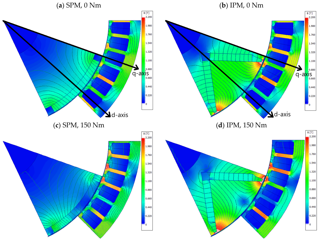
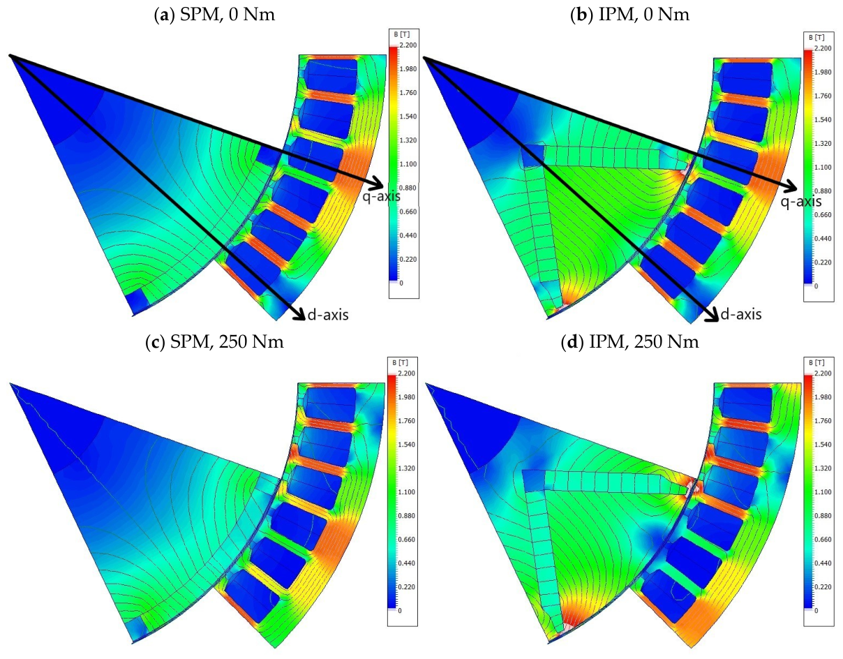
Since the copper losses exhibit an inherently convex dependence on torque, the concavity of the power loss curve related to the inflection point occurrence should be attributed to iron losses. Given that the iron losses are primarily influenced by the magnetic flux density distribution, they are strongly affected by magnetic saturation effects. Thus, the length of IPM motor magnets is chosen by matching the no-load PM flux linkage of both motors, which ensures a similar stator saturation level in no-load conditions (see Figure 4a,b). Thus, the length of IPM motor magnets is chosen by matching the no-load PM flux linkage of both motors, which ensures a similar stator saturation level in no-load conditions (see Figure 4a,b). Due to the differences in rotor geometry, the rotor magnetic flux distribution at the no-load operating point differs between the motors. However, as the stator iron losses dominate the rotor iron losses, the total no-load iron losses are comparable for the two motors. In the IPM motor, longer magnets are needed to compensate for higher flux leakage through rotor bridges.
In the motor load conditions, the torque-production component of the stator current ( I q ) produces an additional magnetomotive force (MMF), which may influence the total magnetic flux density distribution. However, as shown in Figure 4, corresponding to the constant torque region speed of 2000 rpm, the magnetic flux density distribution remains similar for no-load and high-load conditions, both in magnitude and shape. At high load, a certain circumferential flux density shift can be observed compared to no-load conditions, which is caused by the additional MMF in the q-axis, and has a secondary influence on the stator teeth and yoke flux density. Considerable influence is seen in rotor bridges and yoke (Figure 4c), but those are mainly local effects that do not affect the global flux density distribution. These findings confirm that the flux distribution is predominantly governed by the permanent magnets, while the armature reaction introduces only a secondary effect. It is worth noting that, while the rotor bridges are highly saturated (the flux density reaches 2.2 T), the peak flux density in the stator teeth and yoke of both machines is more regular (around 1.85 T).

2.3. FEA Parameters

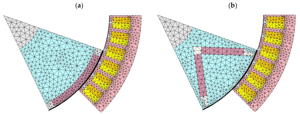
A two-dimensional nonlinear magnetostatic finite element model has been developed to analyze the magnetic flux distribution of the SPM and IPM motors over a full electrical period (360° electrical) in 30 discrete rotor positions. The model was discretized by using 2618 mesh elements for SPM and 2582 elements for IPM motor (Figure 5), using the default mesh size setup in the software. The mesh convergence study is proved in Appendix A. The full list of parameters related to the FEA model is given in Table 5.
In addition, the mapping of motors considered in Section 3.1 is done through a steady-state analysis based on FEA, evaluated point-by-point in the d-q plane. The d-q current mapping is defined by sweeping the current using 10 discrete values ranging from zero to the maximum value defined by the current density of 30   A / m m 2 . For each current magnitude, 8 current phase angles ranging from 0° to 90° are considered, resulting in mapping through 80 operating points in total. The initially predefined 30-point mapping was found to be insufficient, as it did not provide sufficiently smooth maps for magnetic saturation and iron loss evaluation. Therefore, the resolution of the d–q map was increased to 80 points to ensure improved continuity and accuracy in the calculated machine characteristics. As demonstrated in Appendix A, the computational time of the single operating point is approximately 16 s. In the case of parallel map generation using multiple processor cores, the total time for full mapping across 80 operating points requires approximately 900 s on a PC specified in Appendix A.
The copper losses are calculated in Motor-CAD based on conductor resistance and using the common I 2 R relation. The iron losses are modeled through the Steimetz equation, where losses are divided into hysteresis and eddy current losses. To account for the effects of PWM excitation and the increase in losses associated with manufacturing processes (e.g., laser cutting or punching of iron laminations), the calculated iron and permanent magnet losses were scaled up in the model by an empirical correction factor of 2 in the model [33]. The mechanical losses are omitted, as they would be the same for both motor variants and depend on speed rather than torque as an input to the power loss curve of interest. The PM losses are modeled as eddy current losses, using the same approach as for the iron losses.
The FEA workflow used for the construction of motor performance maps was experimentally validated on a 12 kW SPM traction motor available in the laboratory [34]. In this study, the same validated workflow is applied to the SPM and IPM motors, with performance maps constructed with FEA-based mapping in the d–q plane. A summary of the validation results is provided in Appendix B.

3. FEA-Based Motor Performance Maps

3.1. FEA-Based d-q Plane Mapping

The generated maps provide insight into the nonlinear relationship between the current vector in the d-q plane and the PM flux linkage, saliency ratio, and d- and q-axis inductances.
The PMSM electromagnetic torque can be expressed by the following equation, depending on the magnetic flux and d- and q-axis currents [30]
T = 3 2 p ( ψ d I q ψ q I d ) = 3 2 p ( ( ψ P M + L d I d ) I q L q I q I d ) = 3 2 p ( ψ P M I q + ( L d L q ) I q I d ) = T P M + T r e l
where p is the number of pole pairs, ψ d and ψ q are the d- and q-axes flux linkages, and I d and I q are the d- and q-axes currents, with I d being negative under the flux-weakening and reluctance torque production. Note that the difference between L d and L q defines the reluctance torque T r e l , while the PM flux linkage ψ P M   relates to the PM torque component T P M .
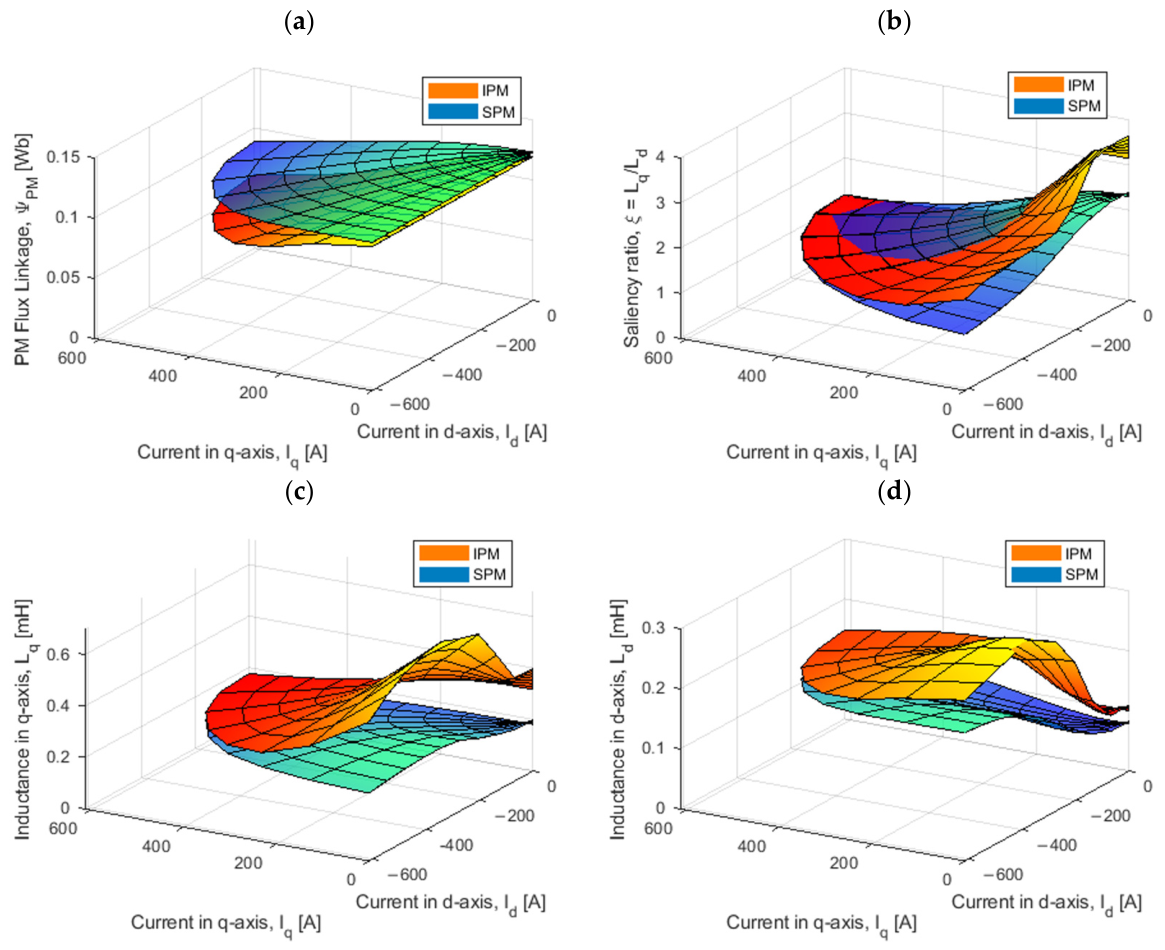
In the non-saturated, non-salient SPM motor, d- and q-axis inductances are theoretically equal since the reluctance defined by the flux linkage path is magnetically equivalent in both d- and q-axis directions [35]. However, in high-performance SPM motors, the permanent magnet MMF is strong enough to form a main path along the d-axis, creating high local flux density and, thus, saturation in the d-axis. In contrast, no significant flux path is observed along the q-axis, besides flux leakage through rotor bridges, thus resulting in lower magnetic flux density in the q-axis (Figure 4a; no magnetic flux lines are observed along the q-axis). The saturation effect is manifested in reducing the relative magnetic permeability of the d-axis and thus its inductance at no-load ( L d   < L q at low I q , see Figure 6c,d, and note that the vertical axes are different therein), producing reluctance torque T r e l > 0 similar to the torque-generating mechanism in IPM motors.
For the IPM motor, besides the difference in L d and L q caused by the different reluctance of the flux linkage paths in d- and q-axes, additional reduction in L d in relation to L q occurs at low I q due to saturation of the d-axis caused by the PM flux linkage (Figure 6c,d). This increase in inductance difference results in an increased reluctance torque capability of the IPM motor (see Equation (1)). Nevertheless, geometry remains the primary source of the IPM motor inductance difference, making the saliency ratio ξ = L q L d higher in the IPM motor variant compared to the SPM variant (Figure 6b).
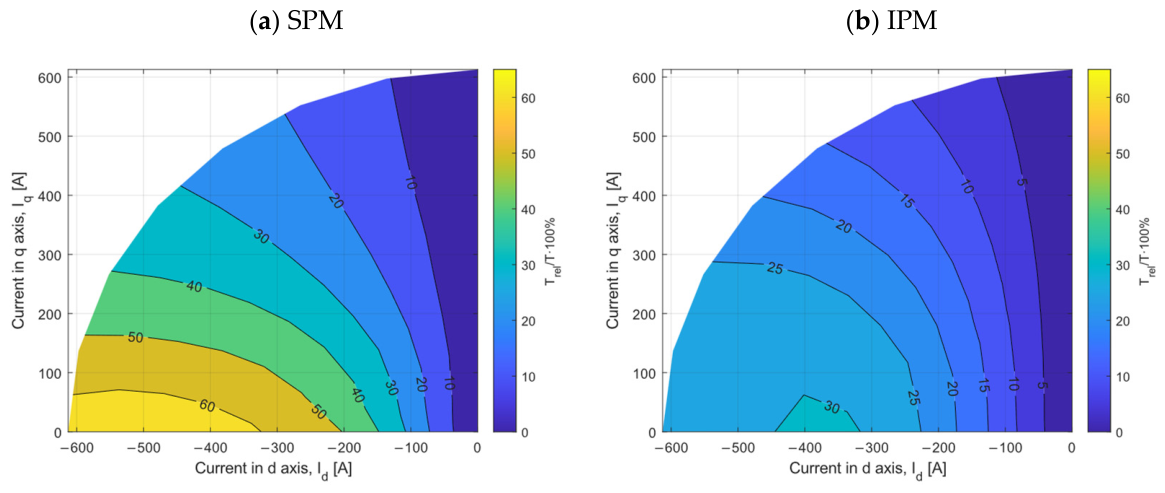
Figure 7 reveals that the share of reluctance torque T r e l in the total electromagnetic torque T increases significantly in the flux weakening region (high | I d | ) for the IPM motor, which is due to the rising difference between L d and L q (cf. Figure 6c,d, and see Equation (1)). In contrast, the share of reluctance torque increases at a much slower rate for the SPM motor, suggesting that flux weakening operation has less effect on L d and L q difference, thus not significantly affecting the torque-generating mechanism.

3.2. Current Allocation Strategies

To address the driving range issue of EVs, the electric motor current components I d and I q should be allocated for maximum efficiency for the given torque T and speed n. The maximum efficiency (ME) optimization problem solved within the Motor CAD environment is defined as [36]
minimize   P l o s s = P C u + P F e + P P M + P m e c h
subject   to   T s h a f t T d e m a n d = 0
and   V l i m   V = 2 π f ψ d 2 + ψ q 2  
where P l o s s is the total motor power losses, including the copper losses P C u , the iron losses P F e , permanent magnet losses P P M , and mechanical losses P m e c h , T s h a f t is the generated motor shaft torque, T d e m a n d is the required torque, and V and V l i m are the actual and maximum phase voltages, respectively.
On the other hand, the MTPA approach (also implemented in Motor CAD) maximizes the motor torque for the given current capacity, thus effectively minimizing the copper losses only
minimize   I s = I d 2 + I q 2
subject   to   T s h a f t T d e m a n d = 0
and   V l i m   V = 2 π f ψ d 2 + ψ q 2  
where I s is the stator phase current. Note that the efficiency map of the motor is strongly influenced by the stator current vector allocation strategy, as optimizing the currents I d and I q influences both torque production and loss mechanisms.

3.3. Power Losses and Efficiency Maps

The motor efficiency and loss maps are generated in the Motor CAD software by applying the particular current control strategy to pre-calculated torque and loss maps in the d-q plane. These maps contain information about the motor’s performance characteristics, and the current control strategy selects the optimal current vector for each torque and speed combination, as described in the previous subsection.
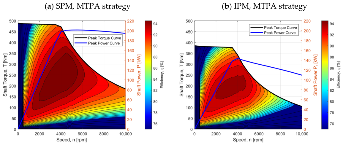
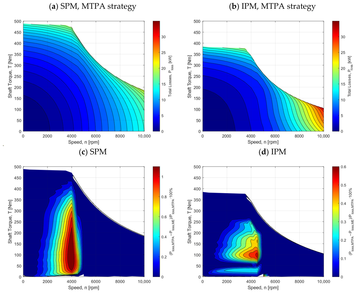
Figure 8 compares the efficiency maps of the SPM and IPM motors under MTPA control. Evidently, the IPM motor exhibits notably lower efficiency in the high-speed/high-torque region. In other words, the IPM motor shows a more confined peak-efficiency area and faster efficiency degradation at high speeds, indicating greater sensitivity to operating conditions. The efficiency maps in the case of ME current control are very similar to those related to MTPA control, with maximum power loss deviation of 1% for both SPM and IPM motors (Figure 9c,d). Hence, only one control strategy (MPTA) may be considered when analyzing power loss.
Although the IPM motor typically offers higher flux-weakening capabilities, which are crucial for EV propulsion, matching the magnetic states of the IPM and SPM under no-load conditions with strong magnets leads to similar flux-weakening performance in the particular case. Since the IPM motor has significantly larger flux leakage, the usable PM flux linkage of the IPM motor is lower than SPM, which leads to lower maximum torque and power despite the higher reluctance torque capability (see Table 6 and Figure 8). As discussed in Section 2, matching the PM flux linkage is useful for ensuring comparable magnetic properties in the no-load condition, allowing a fair comparison of current vector control and power loss behavior as the main subject of this study. However, one should be cautious to avoid misinterpreting conclusions regarding motor performance from such a comparative study.

3.4. Optimal Current Vector Trajectories

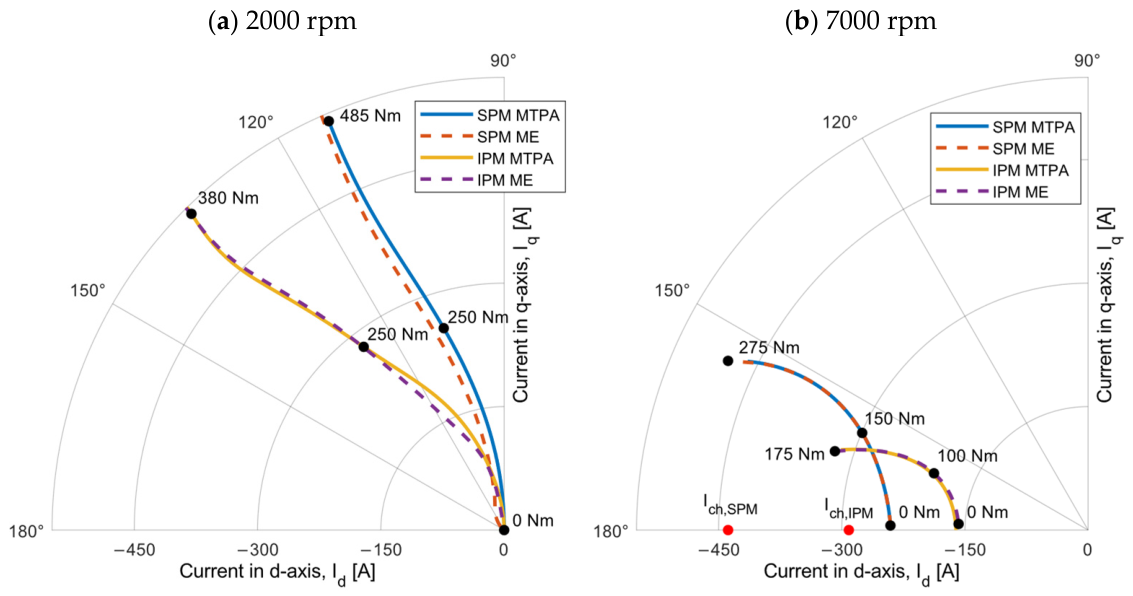
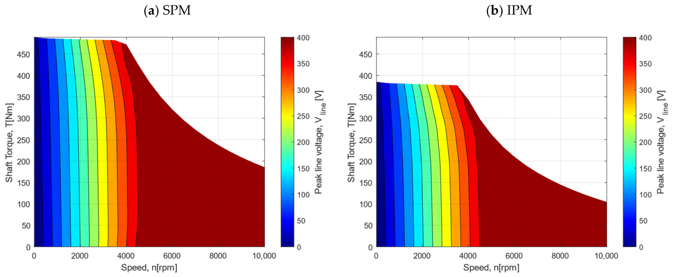
Comparison of SPM and IPM motor optimal current trajectories for both MTPA and ME criteria is shown in Figure 10 for motor speeds of 2000 and 7000 rpm. A certain deviation between MTPA and ME trajectories in the constant torque region (Figure 9a) reflects different optimization objectives (see Equations (2) and (5)). The close agreement between the two sets of trajectories is a consequence of the low sensitivity of iron losses to changes in the current vector under strong PM flux linkage influence (see Figure 3). In the constant torque region, the iron losses at low speed are only weakly dependent on torque (see next section), as they are primarily determined by speed and magnetic flux density through the iron parts. Since the MTPA strategy already optimally allocates current to minimize the copper losses for the required torque, and the iron losses cannot be significantly reduced through further current vector adjustments due to low sensitivity of iron losses to torque, the efficiency benefit of the ME strategy compared to MTPA is low. In the flux-weakening region, both strategies converge to nearly identical trajectories due to the active inverter voltage constraint (see Equations (4) and (7), and illustration in Figure 11). This convergence holds regardless of motor type, but the current vector trajectories of SPM and IPM motors themselves are highly different (Figure 10b).
In the constant torque region, when compared to the SPM motor, the IPM motor is characterized by a higher inductance difference L d L q (see Figure 6c,d) and exploits the reluctance torque more, thus resulting in a larger phase advance angle (more negative I d , Figure 10a). Compared to the IPM, the SPM motor exhibits a higher characteristic current (the current required to cancel the permanent magnet flux; red dots in Figure 9b)
I c h = ψ P M L d
primarily due to its smaller L d . As a result, a relatively large negative I d is required for the SPM motor to counteract the permanent magnet flux during flux-weakening operation (Figure 10b). Since both characteristic currents are smaller than the maximum current (Figure 10b), both motors have theoretically infinite maximum speed (see Figure 8). In contrast, the inductances are much larger in the IPM motor (see Figure 6), which thus reaches the voltage limit with smaller current in the flux-weakening operation for the same speed and equal PM flux linkage than in the case of SPM. As a result, usable I q is reduced, which reduces the achievable maximum torque (see Figure 8 and Figure 10b).

4. Analysis of Inflection Point Occurrence

4.1. Motor Power Loss vs. Torque Curves

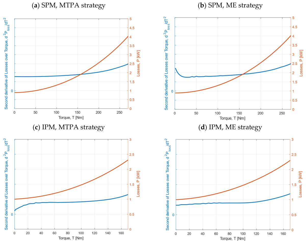
The same motor speeds considered in Section 3 are selected here for analyzing the motor power loss curves. In the loss distribution analysis, PM losses are not treated as a separate loss component because their contribution is relatively small compared to the iron losses. However, they are included in the reported total loss values. At the lower, constant torque region, speed of 2000 rpm, the second power loss derivative over torque is always positive regardless of motor type and control strategy (Figure 12), meaning that the total power loss curve exhibits a strictly convex shape. However, it is worth noting that for the IPM motor, the second derivative experiences a noticeable reduction at low torque values (particularly for the MTPA strategy), which indicates a weaker convexity compared to the SPM motor.
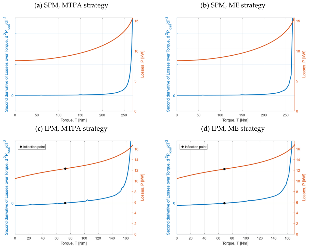
For the higher flux weakening region speed of 7000 rpm, the IPM motor power loss curve does include the inflection point for both MTPA and ME strategies, in which the second derivative of the power loss curve crosses zero (designated by black dots in Figure 13c,d). Because of very similar current vector paths in the d-q frame (see Figure 9b), the power loss curves and their second derivatives are very similar for the two current vector control strategies. On the other hand, the power loss curve is strictly convex for SPM (Figure 13a,b), i.e., it does not include the inflection point. Note that the presence of an inflection point in the power loss curve only beyond a certain speed has been experimentally observed in [18].

4.2. Power Loss Distribution Analysis

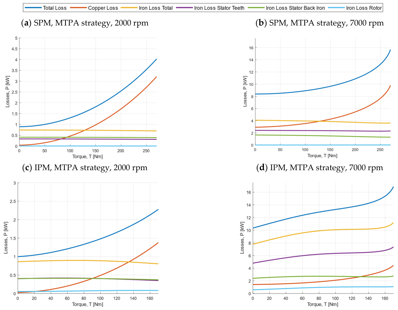
The power loss curve should have a concave shape (i.e., the negative second derivative) in the low torque region to include the inflection point. Since the copper losses are strictly convex with respect to torque/current, the loss curve concavity can only come from the iron loss contribution, which is determined by the magnetic flux density distribution. For the total power loss curve to be concave, the iron loss curve’s concavity should overcome the copper loss curve’s convexity. Even at lower speeds, the iron loss curve may be concave both for the SPM and IPM motor, but this concavity is too weak to overcome the copper loss curve convexity (see Figure 14a,c). Due to the approximately quadratic increase of iron losses with electrical frequency (and thus the motor speed), as described by the Bertotti equation [37], the iron losses and their concavity may become dominant in the high-speed, flux-weakening region (see Figure 14d for the IPM motor). Since the SPM motor employs higher current in the flux-weakening region (see Figure 10b), the SPM copper losses are much higher, leading to less likely iron loss dominance (Figure 14b).
Figure 14b,d further indicate that the dominant contribution to total iron losses of both motors in the flux-weakening region comes from the stator teeth. As the torque increases, the growth of stator teeth losses becomes increasingly pronounced for the IPM motor (Figure 14d), and it closely follows the mixed concave and convex trend of the total loss curve. In other words, the inflection point of the total power loss curve coincides with the inflection point occurring in the stator teeth loss curve. Other components, such as the stator back iron and rotor losses, remain smaller and are not significantly influenced by torque (no distinct inflection point occurred; Figure 14). A detailed analysis of the stator teeth’s iron loss is presented in the next subsection.

4.3. Flux Saturation Analysis

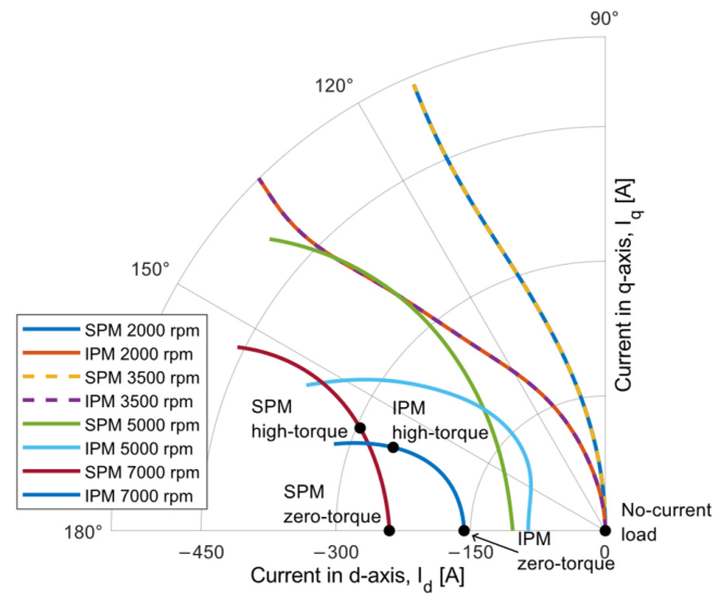
In both motors, permanent-magnet flux linkage dominates, while the d- and q-axis current contributions to flux are of secondary importance. At lower speeds, the absence of voltage constraint (see Equation (4)) allows the current vector trajectory to remain in its unconstrained, speed-independent optimal position (see trajectories in Figure 15 corresponding to 2000 and 3500 rpm), thus resulting in a constant magnetic state across multiple speeds. Above the corner speed of around 4000 rpm (see Figure 8), the voltage constraint forces the current vector away from the constant torque region into the flux-weakening region. Since the magnetic flux distribution, and thus saturation of iron parts, depends on the current vector position, this flux weakening current vector shift has a direct impact on inductances and flux distribution.
In the constant-torque no-current/no-load conditions, both motors experience similar iron saturation effects, as shown in Figure 4a,b. In the flux-weakening region, the no-current load point is beyond the voltage limit (so, unfeasible), and is used in the analysis as a magnetic state reference operating point, in addition to the feasible zero-torque point (see Figure 15 for n > 4000 rpm). For meaningful comparison of flux-weakening and torque generation influence on flux saturation, the high-torque operating point (150 Nm) is considered, as well. For the zero-torque point, only negative I d current component exists ( I q = 0 , see Equation (1)), which effectively reduces the PM flux linkage and puts the operating point within the voltage limit.
Compared to no-current load operating points at 2000 rpm (Figure 4a,b), both SPM and IPM experience lower magnetic flux density values across iron parts at the zero-torque point at 7000 rpm (cf. Figure 16a,b and Figure 4a,b). At higher torques, the SPM motor exhibits even higher reduction in magnetic flux density globally (Figure 16c), despite localized regions of higher saturation. This is reflected in the falling total iron loss curve with respect to torque increase (Figure 14b). As the torque increases, the current vector shifts from purely negative I d toward higher I q (see Figure 15, 7000 rpm). In the IPM motor, the high q-axis inductance L q (Figure 6c) results in a significant q-axis flux contribution when the torque-production current I q is applied at high speeds in addition to the flux-weakening current I d < 0 . The iron parts in the q-axis turn out to saturate quicker than the d-axis. Flux weakening reduces the overall magnetic flux, thus resulting in locally increasing magnetic flux density with rising torque despite operating in the flux weakening region (cf. Figure 16b,d). The corresponding quantitative results in Table 7 indicate that the SPM motor inductances L d and L q are barely influenced by the torque shift. This shift corresponds to a small reduction in the d-axis flux while generating a certain amount of q-axis flux. The IPM motor has approximately two times larger L q than the SPM motor (Table 7), so that around twice the amount of q-axis flux is produced with a somewhat lower I q current. Furthermore, because the IPM motor has a larger L d , as well, a smaller I d current is required to achieve a significantly greater d-axis flux reduction. In addition, because the permanent magnets are embedded deeper within the rotor, the d-axis current can produce a larger demagnetizing effect, resulting in a greater reduction in the d-axis effective flux for a given I d current (Figure 15). In summary, as the torque increases, both the reduction in flux linkage in the d-axis and the increase in flux linkage in the q-axis are stronger for the IPM motor compared to the SPM motor for the same voltage limit (Table 7).
Table 8 and Table 9 present the loss distribution for the three characteristic motor load operating points for the motor speed of 7000 rpm. In the SPM motor, the total iron losses decrease from the no-current load point through the zero-torque point to the load point (see Table 8 and Figure 14b), as the larger negative I d reduces the air-gap flux. In contrast, the IPM motor exhibits a non-monotonic behavior of the total iron losses, including the inflection point (see Table 9 and Figure 14d). The iron losses decrease slightly at the zero-torque point with decreased flux in the d-axis, while rising significantly at the load point as the I q current additionally saturates the stator teeth (Figure 16d). This indicates that in the IPM motor, the q-axis flux saturation in the flux weakening region has a major influence on the iron losses, dominating the flux reduction produced by the negative I d , and shaping the (iron) loss curve to become concave.

5. Optimal Torque Distribution in Multi-Motor Electric Vehicles

5.1. Torque Distribution Optimization

Offline optimization of the EV torque distribution across the entire vehicle operating range represents a key step in designing an online torque distribution control strategy [5,25]. By defining the torque split ratio as
σ = T f T t = T f T f + T r
The front and rear axle torques can be expressed as
T f = σ T t
T r = ( 1 σ ) T t
where T t is the total torque demand for an EV with four equal in-wheel motors, subject to straight-line driving. It should be noted that for straight-line driving conditions, the four in-wheel motor configuration is equivalent to the dual-motor configuration from Figure 1, because of the equal speeds and torques of the left and right motors of the same axle [6]. The optimization is aimed at minimizing the total electric power (i.e., battery power) consumption, including the total EV motor losses
P e = 2 P l o s s 1 ( | n | , σ | T t | / 2 ) + 2 P l o s s 2 ( | n | , ( 1 σ ) | T t | / 2 )
where P l o s s 1 and P l o s s 2 are power loss maps of front- and rear-axle motors, respectively, and n is the motor speed. By taking the absolute values of motor torque (and speed) inputs in Equation (12), the power loss maps obtained through the FEA model (Figure 9a,b) are used in the regenerative braking operating model, as well.
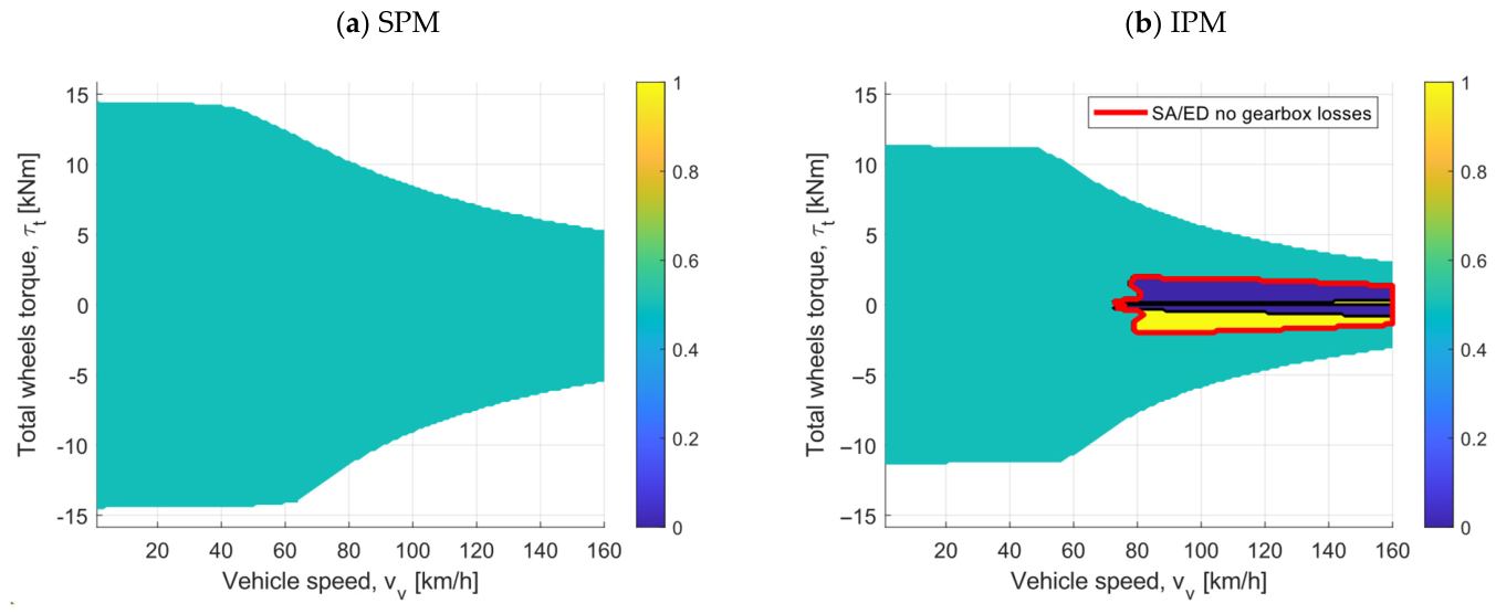
The optimization has been conducted separately for the MTPA strategy-controlled SPM and IPM power loss maps from Figure 9a and Figure 9b, respectively, by using a grid search approach for the torque split ratio step of 0.01. The backward-looking vehicle model was adopted from [5], and it includes the acceleration-dependent front/rear axle load shift and longitudinal tire friction losses. The motor gearbox losses are excluded (see next subsection for analysis of their influence). The optimization results shown in Figure 17b for the IPM motor clearly indicate the split between SA ( σ = 1 or σ = 0 ) and ED operation ( σ = 0.5 ) in the high-speed (flux weakening region, which is the consequence of inflection point occurrence in the power loss maps of this motor (Figure 14d). Note that the SA operation minimum vehicle velocity of around 75 km/h corresponds to the motor speed of 4500 rpm (for the effective tire radius of 0.317 m and gearbox ratio of 7.5), which is close to the motor corner speed of 4000 rpm according to Figure 8b. The SA operation relates to the front ( σ = 1 ) or rear axle ( σ = 0 ) depending on whether the vehicle decelerates or accelerates, respectively, which relates to the minimization of longitudinal tire losses, as described in [5]. Since the SPM motor power loss curve does not include the inflection point (see Figure 12a and Figure 13a), the torque distribution reduces to ED in virtually the whole operating range (Figure 17a).

5.2. Influence of Gearbox Power Losses on Optimal Torque Distribution

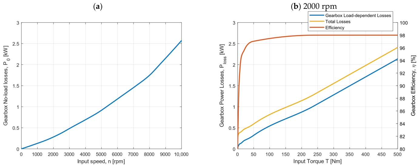
The gearbox losses are divided into no-load (idling) speed-dependent losses (Figure 18a) and load-dependent losses obtained from the gearbox efficiency curve (Figure 18b). The model has been adopted from [5], where it was created based on the model used in [38] and references cited therein. The total gearbox loss model reads
P l o s s f , r = P 0 ( n w ) + T w f , r n w π 30 ( 1 η ( T w f , r ) 1 )
where P 0 are no-load speed-dependent losses (Figure 18), T w f , r and n w are the wheel torque and speed, respectively, and η is the gearbox efficiency, which is torque-dependent (Figure 18b).
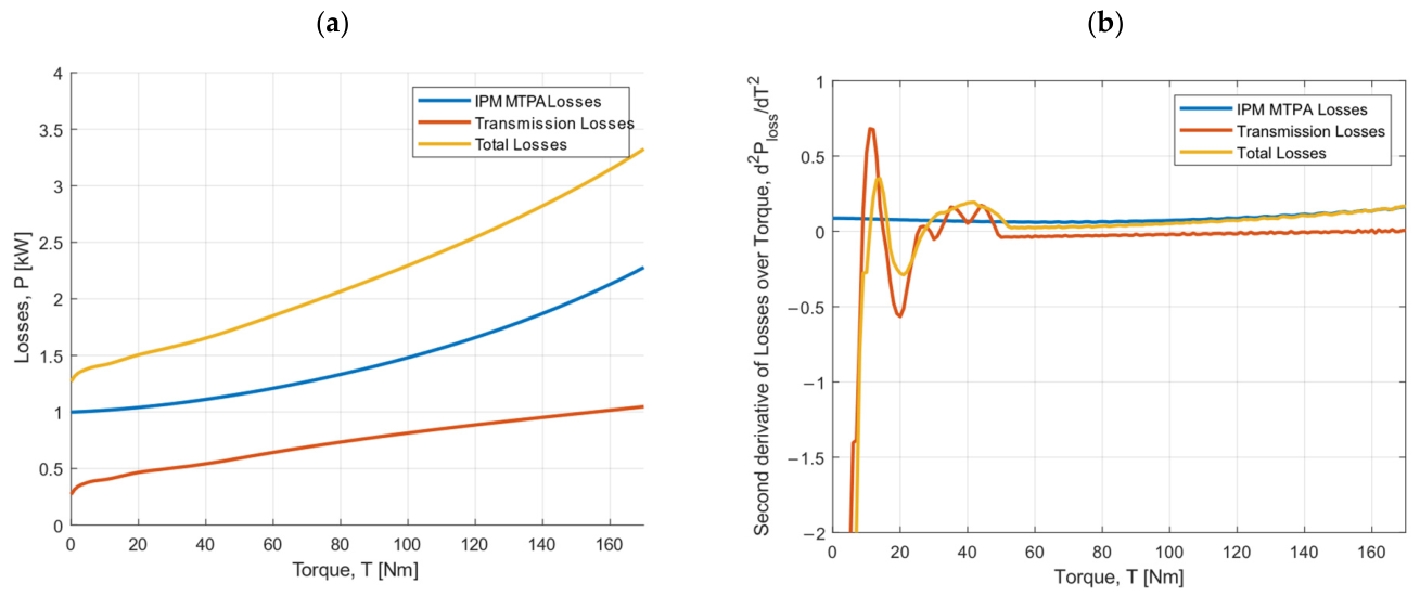
Since the power loss curve of interest is defined in dependence on torque (see Figure 12), only the load-dependent losses (Figure 18b) are relevant for the inflection point occurrence analysis. The zoom-in view of Figure 18b, shown in Figure 19a, indicates that the gearbox loss curve is concave in the low torque range (and accordingly, the second derivative curve is negative, Figure 19b). This makes the total geared IPM motor curve concave even in the constant torque region, at a speed of 2000 rpm, where the motor power curve itself is convex. The gearbox power loss curve concavity (Figure 19a) comes from the rising shape of the efficiency vs. load curve (Figure 18b), which may be explained by the falling normal load-dependence of the coefficient of friction for the gear tooth sliding friction contact.
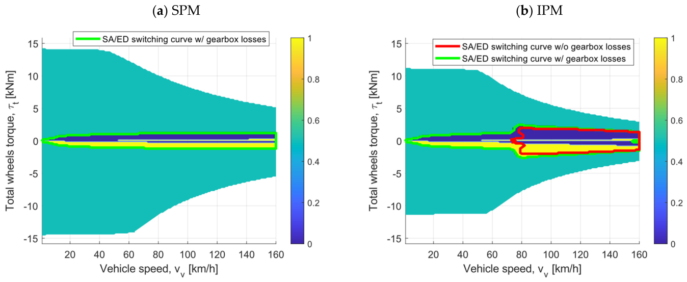
Thus, at low loads, it is more efficient to use only one axle to propel the EV, focusing all torque on a single gearbox. The low efficiency of the reduction gearbox also affects optimal torque vectoring in both SPM (Figure 20a) and IPM (Figure 20b) propulsion systems. Shape of switching torque curve for SPM motors (labeled with green lines in Figure 20a), which shows a region that becomes wider up to medium speeds and then becomes nearly constant, also matches the measurements in [18]. In the case of the IPM motors, the switching torque curve is influenced by both effects. At lower speeds, the influence of gearbox losses is clearly visible, whereas at higher speeds, the IPM-induced switching torque curve becomes dominant. Since the IPM motor alone exhibits a wider switching torque curve range, the influence of the gearbox, dominant mainly at lower torque levels, can be considered negligible. When compared to an IPM motor-powered EV without a modeled gearbox, the SA area now covers a wider area through all speeds and becomes wider than the SA area without a gearbox (Figure 17b). This expansion makes the SA/ED torque distribution strategy more effective than the basic ED strategy.
The concavity of the gearbox power loss curve in the low torque region (Figure 19a) is manifested in the appearance of the SA mode for the SPM motor-propelled EV (cf. Figure 17a and Figure 20a). The switching torque curve, shown by the green line in Figure 20a, becomes wider up to medium vehicle velocities and then becomes nearly constant, which matches the results gained from recorded motor loss maps in [39]. In the case of IPM motors, the SA mode appears in the low-mid velocity range (cf. Figure 17b and Figure 20b), and the switching curve is comparable to the case of SPM motors. In the high-velocity range, the switching curve is only slightly shifted up in the presence of gearbox losses (cf. green and red lines in Figure 20b), which is because the motor loss curve concavity dominates the gearbox one.

6. Conclusions

A finite element analysis (FEA) has been carried out to investigate the experimentally observed occurrence of an inflection point in the power loss vs. torque curve of permanent magnet synchronous motors (PMSM) of different types (SPM vs. IPM) and current control strategies (MTPA vs. ME). The corresponding profile of optimized torque distribution among multiple motors of an AWD electric vehicle (EV) has been analyzed, as well.
The FEA has been shown to be capable of reproducing the power loss inflection point for the IPM motor in the flux-weakening region. The concave shape of the power loss curve in the low torque region, needed for inflection to exist, has been found to be induced by iron losses, mostly in saturated stator iron teeth. Due to the high q-axis inductance of the IPM motor, a significant q-axis flux contribution is generated under torque-production current in the high-speed, flux-weakening region. Thus, the total magnetic flux is increasingly dominated by the q-axis saturation, which outweighs the flux-weakening contribution of the negative d-axis current. This leads to a net increase in magnetic flux density with increasing torque in the flux-weakening region, resulting in a concave shape of the iron loss curve. On the other hand, in the case of SPM motor operating in the flux-weakening region, lower q-axis inductance limits the flux that q-axis current generates, while the reduced reluctance torque capability suppresses the q-axis current itself, thereby resulting in a decrease in the total magnetic flux with torque, with no inflection point occurring in the iron loss and thus the total loss curve.
The EV transmission loss has been identified as an additional source of low-torque concavity of the total power loss curve and, thus, a contributor to the occurrence of an inflection point. This effect is caused by the rising trend of the transmission efficiency curve in the low torque region, which reduces the rate of power loss increase with torque, i.e., gives the concave shape of the power loss curve. The optimized front/rear-axle torque distribution map aligns with equal distribution (ED) in the case of the SPM motor and ideal (no-loss) transmission, i.e., in the case of a convex motor power loss curve. Incorporating the transmission loss model introduces the single-axle (SA) operation across the full vehicle speed range, with the SA-ED torque switching curve following a saturated rising trend with velocity. In the case of an IPM motor, the SA region broadens, i.e., the torque switching curve lifts in the flux weakening-related high velocity region due to the contribution of the IPM motor electric power loss curve concavity contribution.
The future work can be directed to (i) analyzing power inverter loss influence, (ii) applying 3D FEA methodology for a more accurate representation of different power loss effects, (iii) applying FEA to characterize induction motor power losses, and (iii) developing a lumped-parameter SMPM model capable of capturing the power loss curve inflection point.


Author Contributions

Conceptualization, I.G., Z.H. and J.D.; methodology, I.G., Z.H. and J.D.; software, I.G. and Z.H.; validation, I.G. and Z.H.; formal analysis, I.G., Z.H. and J.D.; investigation, I.G.; resources, Z.H. and J.D.; data curation, I.G.; writing—original draft preparation, I.G.; writing—review and editing, Z.H. and J.D.; visualization, I.G.; supervision, Z.H. and J.D.; project administration, J.D. All authors have read and agreed to the published version of the manuscript.

Funding

This research received no external funding.

Data Availability Statement

Requests to access the datasets should be directed to Joško Deur at josko.deur@fsb.unizg.hr.

Conflicts of Interest

The authors declare no conflicts of interest.

Abbreviations

The following abbreviations are used in this manuscript:
4AWDFour Wheel Drive
EDEqual Distribution
EVElectric Vehicle
FEAFinite Element Analysis
IPMInterior Permanent Magnet
MEMaximum Efficiency
MTPAMaximum Torque per Ampere
PCPersonal Computer
PMSMPermanent Magnet Synchronous Motor
PWMPulse Width Modulation
SASingle-Axle
SPMSurface Permanent Magnet

Appendix A

A mesh convergence analysis was performed to verify the applied FEA setting presented in Section 2. Three mesh configurations were evaluated for the operating point of 2000 rpm and 150 Nm, which correspond to maximum finite element size of (i) the default value (used in the paper; expectedly larger than 1 mm), (ii) 1 mm, and (iii) 0.5 mm. The results shown in Table A1 indicate that the copper losses are insensitive to mesh refinement, while the stator and rotor iron losses exhibit minor sensitivity to mesh size (lower than 1% and 5%, respectively). The magnet losses show the strongest sensitivity (around 15%); however, their absolute contribution is small compared to iron losses (see Table A1). On the other hand, the model execution time increases substantially when increasing the mesh resolution. This analysis confirms that the applied (default) mesh resolution represents a suitable compromise between the simulation accuracy and execution speed.
Table A1. Influence of maximum finite element size on calculated SPM motor losses and related execution time.
ParameterDefault1 mm0.5 mm
Copper losses [W]937.7937.7 (0%)937.7 (0%)
Stator iron losses [W]756.1759.8 (+0.5%)758.5 (+0.3%)
Rotor iron losses [W]82.084.6 (+3.2%)78.2 (−4.6%)
Magnet losses [W]6.06.9 (+15%)7.0 (+16.7%)
Execution time [s] *1632 (+100%)72 (+350%)
* Execution time per operating point. CPU used: 4 × AMD EPYC 7713 (64 cores, 2.00 GHz), RAM: 48 GB.
Appendix B

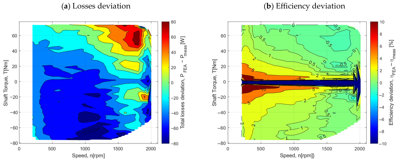
The numerical electromagnetic workflow used in this study was first experimentally validated for a 12 kW SPM machine available in the laboratory, as described in detail in [34]. Figure A1a presents the absolute deviation between simulated and measured motor power losses. For most of the operating range, the absolute deviation is within approximately 40 W on the full-scale output of 880 W, while larger deviations (up to 80 W) are visible only at higher torques in both motoring and regenerative braking regimes. The corresponding maximum relative deviation is 9%. In terms of motor efficiency deviation (Figure A1b), it is within 1% of difference in most of the operating range, and rises closer to the plot axes, mostly due to the growing influence of measurement uncertainties. These results confirm that the finite-element modeling method applied in the paper can reproduce the measured power losses with good accuracy.
Figure A1. Deviations between simulated and measured total losses (a) and efficiency (b) of the tested 12 kW SPM motor.
Energies 19 03040 g0a1

References

  1. IEA. Global EV Outlook 2025; IEA: Paris, France, 2025. Available online: https://www.iea.org/reports/global-ev-outlook-2025 (accessed on 12 February 2026).
  2. Allca-Pekarovic, A.; Kollmeyer, P.; Middleton, M.; Emadi, A. A Review of Production Multi-Motor Electric Vehicles and Energy Management and Model Predictive Control Techniques. In Proceedings of the WCX SAE World Congress Experience, Detroit, MI, USA, 16–18 April 2024. [Google Scholar]
  3. Mutoh, N.; Kazama, T.; Takita, K. Driving characteristics of an electric vehicle system with independently driven front and rear wheels. IEEE Trans. Ind. Electron. 2006, 53, 803–813. [Google Scholar] [CrossRef]
  4. Koehler, S.; Viehl, A.; Bringmann, O.; Rosenstiel, W. Energy-efficiency optimization of torque vectoring control for battery electric vehicles. IEEE Intell. Transp. Syst. Mag. 2017, 9, 59–74. [Google Scholar] [CrossRef]
  5. Gruber, P.; Sorniotti, A.; Lenzo, B.; De Filippis, G.; Fallah, S. Energy efficient torque vectoring control. In Advanced Vehicle Control; CRC Press: Boca Ration, FL, USA, 2016; pp. 117–122. [Google Scholar]
  6. Škugor, B.; Deur, J.; Chen, W.; Zhang, Y.; Dai, E. Optimization of straight-line driving torque vectoring for energy-efficient operation of electric vehicles with multiple motors and disconnect clutches. Optim. Eng. 2025, 26, 753–780. [Google Scholar] [CrossRef]
  7. Xu, Y.; Kersten, A.; Klacar, S.; Ban, B.; Hellsing, J.; Sedarsky, D. Improved efficiency with adaptive front and rear axle independently driven powertrain and disconnect functionality. Transp. Eng. 2023, 13, 100192. [Google Scholar] [CrossRef]
  8. Gong, C.; Li, Y.R.; Zargari, N.R. An Overview of Advancements in Multimotor Drives: Structural Diversity, Advanced Control, Specific Technical Challenges, and Solutions. Proc. IEEE 2024, 112, 184–209. [Google Scholar] [CrossRef]
  9. Nguyen, C.T.P.; Nguyễn, B.-H.; Ta, M.C.; Trovão, J.P.F. Dual-motor dual-source high performance EV: A comprehensive review. Energies 2023, 16, 7048. [Google Scholar] [CrossRef]
  10. Wu, D.; Li, Y.; Zhang, J.; Du, C. Torque distribution of a four in-wheel motors electric vehicle based on a PMSM system model. Proc. Inst. Mech. Eng. Part D J. Automob. Eng. 2017, 232, 1828–1845. [Google Scholar] [CrossRef]
  11. Yuan, X.; Wang, J. Torque distribution strategy for a front- and rear-wheel-driven electric vehicle. IEEE Trans. Veh. Technol. 2012, 61, 3365–3374. [Google Scholar] [CrossRef]
  12. Li, Y.; Zhang, J.; Guo, K.; Wu, D. Optimized torque distribution algorithm to improve the energy efficiency of 4WD electric vehicle. In SAE 2014 Commercial Vehicle Engineering Congress; SAE International: Warrendale, PA, USA, 2014. [Google Scholar]
  13. Song, Z.; Hofmann, H.; Li, J.; Wang, Y.; Lu, D.; Ouyang, M.; Du, J. Torque distribution strategy for multi-PMSM applications and optimal acceleration control for four-wheel-drive electric vehicles. J. Dyn. Syst. Meas. Control 2020, 142, 021001. [Google Scholar]
  14. Fujimoto, H.; Harada, S. Model-based range extension control system for electric vehicles with front and rear driving–braking force distributions. IEEE Trans. Ind. Electron. 2015, 62, 3245–3254. [Google Scholar] [CrossRef]
  15. Sun, B.; Gao, S.; Ma, C.; Li, J. System power loss optimization of electric vehicle driven by front and rear induction motors. Int. J. Automot. Technol. 2017, 19, 121–134. [Google Scholar] [CrossRef]
  16. Da, W.; Bo, W. Research on driving force optimal distribution and fuzzy decision control system for a dual-motor electric vehicle. In Proceedings of the 34th Chinese Control Conference (CCC); IEEE: Piscataway, NJ, USA, 2015; pp. 8146–8153. [Google Scholar]
  17. De Filippis, G.; Lenzo, B.; Sorniotti, A.; Sannen, K.; De Smet, J.; Gruber, P. On the energy efficiency of electric vehicles with multiple motors. In Proceedings of the 2016 IEEE Vehicle Power and Propulsion Conference (VPPC); IEEE: Piscataway, NJ, USA, 2016; pp. 1–6. [Google Scholar]
  18. Zhang, X.; Gohlich, D.; Li, J. Energy-efficient toque allocation design of traction and regenerative braking for distributed drive electric vehicles. IEEE Trans. Veh. Technol. 2017, 67, 285–295. [Google Scholar] [CrossRef]
  19. Lin, C.; Xu, Z. Wheel torque distribution of four-wheel-drive electric vehicles based on multi-objective optimization. Energies 2015, 8, 3815–3831. [Google Scholar] [CrossRef]
  20. Wang, J.; Zhang, C.; Guo, D.; Yang, F.; Zhang, Z.; Zhao, M. Drive-cycle-based configuration design and energy efficiency analysis of dual-motor 4WD system with two-speed transmission for electric vehicles. IEEE Trans. Transp. Electrif. 2023, 10, 1887–1899. [Google Scholar]
  21. Roscher, M.A.; Michel, R.; Leidholdt, W. Improving energy conversion efficiency by means of power splitting in dual drive train EV applications. Int. J. Veh. Technol. 2013, 2013, 398361. [Google Scholar] [CrossRef]
  22. Grđan, I.; Škugor, B.; Deur, J. Energy-efficient straight-line driving torque vectoring for electric vehicles with disconnect clutches and unequal front/rear motors. In Proceedings of the 16th International Symposium on Advanced Vehicle Control (AVEC 2024); Springer: Cham, Switzerland, 2024; pp. 364–370. [Google Scholar]
  23. De Filippis, G.; Lenzo, B.; Sorniotti, A.; Gruber, P.; De Nijs, W. Energy-efficient torque-vectoring control of electric vehicles with multiple drivetrains. IEEE Trans. Veh. Technol. 2018, 67, 4702–4715. [Google Scholar] [CrossRef]
  24. Dizqah, A.M.; Lenzo, B.; Sorniotti, A.; Gruber, P.; Fallah, S.; De Smet, J. A fast and parametric torque distribution strategy for four-wheel-drive energy-efficient electric vehicles. IEEE Trans. Ind. Electron. 2016, 63, 4367–4376. [Google Scholar] [CrossRef]
  25. Lin, C.; Liang, S.; Chen, J.; Gao, X. A multi-objective optimal torque distribution strategy for four in-wheel-motor drive electric vehicles. IEEE Access 2019, 7, 64627–64640. [Google Scholar] [CrossRef]
  26. Chatzikomis, C.; Zanchetta, M.; Gruber, P.; Sorniotti, A.; Modic, B.; Motaln, T.; Blagotinsek, L.; Gotovac, G. An energy-efficient torque-vectoring algorithm for electric vehicles with multiple motors. Mech. Syst. Signal Process. 2019, 128, 655–673. [Google Scholar] [CrossRef]
  27. Wang, R.; Chen, Y.; Feng, D.; Huang, X.; Wang, J. Development and performance characterization of an electric ground vehicle with independently actuated in-wheel motors. J. Power Sources 2011, 196, 3962–3971. [Google Scholar] [CrossRef]
  28. Zheng, P.; Liu, W.; Gao, Y.; Tong, C.; Sui, Y. Review of Fault Diagnosis and Fault-Tolerant Control Technologies for Permanent-Magnet Synchronous Machine. CES Trans. Electr. Mach. Syst. 2025, 9, 320–339. [Google Scholar] [CrossRef]
  29. Künzler, M.; Pflüger, R.; Lehmann, R.; Werner, Q. Dimensioning of a permanent magnet synchronous machine for electric vehicles according to performance and integration requirements. Automot. Engine Technol. 2022, 7, 97–104. [Google Scholar] [CrossRef]
  30. Ahmad, M.Z.; Sulaiman, E.; Haron, Z.A.; Kosaka, T. Preliminary studies on a new outer-rotor permanent magnet flux switching machine with hybrid excitation flux for direct drive EV applications. In Proceedings of the 2012 IEEE International Conference on Power and Energy (PECon); IEEE: Piscataway, NJ, USA, 2012; pp. 928–933. [Google Scholar]
  31. Tang, J.; Liu, Y. Design and Experimental Verification of a 48 V 20 kW Electrically Excited Synchronous Machine for Mild Hybrid Vehicles. In Proceedings of the 2018 XIII International Conference on Electrical Machines (ICEM); IEEE: Piscataway, NJ, USA, 2018; pp. 649–655. [Google Scholar] [CrossRef]
  32. Ghahfarokhi, P.S.; Podgornovs, A.; Kallaste, A.; Cardoso, A.J.M.; Belahcen, A.; Vaimann, T. The oil spray cooling system of automotive traction motors: The state of the art. IEEE Trans. Transp. Electrif. 2022, 9, 428–451. [Google Scholar] [CrossRef]
  33. Boglietti, A.; Cavagnino, A.; Ionel, D.M.; Popescu, M.; Staton, D.A.; Vaschetto, S. A general model to predict the iron losses in pwm inverter-fed induction motors. IEEE Trans. Ind. Appl. 2010, 46, 1882–1890. [Google Scholar] [CrossRef]
  34. Grđan, I.; Hanić, Z.; Deur, J. Experimental Investigation and Modeling of Power Losses in the Bread Loaf Surface Permanent Magnet Synchronous Machine. In Proceedings of the 2025 International Conference on Electrical Drives and Power Electronics (EDPE); IEEE: Piscataway, NJ, USA, 2025; pp. 1–5. [Google Scholar]
  35. Hendershot, J.R.; Miller, T. Design of Brushless Permanent-Magnet Motors; Oxford University Press (OUP): Oxford, UK, 1995. [Google Scholar]
  36. Goss, J.; Popescu, M.; Staton, D.; Wrobel, R.; Yon, J.; Mellor, P. A comparison between maximum torque/ampere and maximum efficiency control strategies in IPM synchronous machines. In Proceedings of the 2014 IEEE Energy Conversion Congress and Exposition (ECCE); IEEE: Piscataway, NJ, USA, 2014; pp. 2403–2410. [Google Scholar]
  37. Lin, D.; Zhou, P.; Fu, W.; Badics, Z.; Cendes, Z. A dynamic core loss model for soft ferromagnetic and power ferrite materials in transient finite element analysis. IEEE Trans. Magn. 2004, 40, 1318–1321. [Google Scholar] [CrossRef]
  38. Deur, J.; Cipek, M.; Škugor, B.; Petrić, J. Modeling and low-level control of range extended electric vehicle dynamics. In Proceedings of the International Conference on Powertrain Modelling and Control (PMC2012), West Yorkshire, UK, 4–6 September 2012. [Google Scholar]
  39. Koehler, S.; Viehl, A.; Bringmann, O.; Rosenstiel, W. Energy-efficient torque distribution for axle-individually propelled electric vehicles. In Proceedings of the 2014 IEEE Intelligent Vehicles Symposium Proceedings; IEEE: Piscataway, NJ, USA, 2014; pp. 1109–1114. [Google Scholar]
Figure 1. Principal schematic of EV powertrain with multi-motor AWD propulsion [9].
Energies 19 03040 g001
Figure 2. Illustration of convex (a) and non-convex (b) power loss functions and their first and second derivatives, including designation of energy-efficient SA and ED operating points, inflection point, and switching point.
Energies 19 03040 g002
Figure 3. Geometry of modeled SPM (a) and IPM motors (b).
Energies 19 03040 g003
Figure 4. Magnetic flux density distribution for SPM and IPM motors in no-load (0 Nm) and load conditions (250 Nm) for a motor speed of 2000 rpm.
Energies 19 03040 g004
Figure 5. FEA mesh of SPM (a) and IPM motors (b).
Energies 19 03040 g005
Figure 6. Comparison of PM flux linkage (a), saliency ratio (b), and q- (c) and d-axis inductances (d).
Energies 19 03040 g006
Figure 7. Reluctance torque percentage share to total electromagnetic torque of SPM (a) and IPM motors (b).
Energies 19 03040 g007
Figure 8. Efficiency maps of SPM (a) and IPM motors (b) controlled via MTPA strategy.
Energies 19 03040 g008
Figure 9. Power loss maps of SPM (a) and IPM motors (b) controlled via MTPA strategy, and relative difference in power losses between MTPA and ME control strategies for SPM (c) and IPM motors (d).
Energies 19 03040 g009
Figure 10. MTPA- and ME-optimized stator current trajectories in d-q reference frame for IPM and SPM motors at speeds of 2000 rpm (a) and 7000 rpm (b).
Energies 19 03040 g010
Figure 11. Comparison of peak line voltages of SPM (a) and IPM motors (b).
Energies 19 03040 g011
Figure 12. The power loss vs. torque curves and their second derivatives for SPM and IPM motors and MTPA and ME current control strategies for motor speed of 2000 rpm.
Energies 19 03040 g012
Figure 13. The power loss vs. torque curves and their second derivatives for SPM and IPM motors and MTPA and ME current control strategies for motor speed of 7000 rpm.
Energies 19 03040 g013
Figure 14. Power loss distribution of MTPA strategy-controlled SPM and IPM motors at speeds of 2000 and 7000 rpm.
Energies 19 03040 g014
Figure 15. Stator current vector trajectories in d-q reference frame for SPM and IPM motors for multiple speeds across constant torque (below 4000 rpm) and flux weakening regions (above 4000 rpm).
Energies 19 03040 g015
Figure 16. Magnetic flux density distribution of SPM and IPM motors in different torque operating points and at a speed of 7000 rpm.
Energies 19 03040 g016
Figure 17. Torque distribution optimization results for four equal SPM (a) and IPM motors (b) controlled via MTPA strategy (no gearbox losses included).
Energies 19 03040 g017
Figure 18. Gearbox no-load losses (a) and load-dependent efficiency and related losses at 2000 rpm (b).
Energies 19 03040 g018
Figure 19. Load-dependent power loss contributions of IPM motor and gearbox (a) and related second derivative curve (b) for reduced torque axis and speed of 2000 rpm.
Energies 19 03040 g019
Figure 20. Torque distribution optimization results for four equal SPM (a) and IPM motors (b) controlled via MTPA strategy (gearbox losses included).
Energies 19 03040 g020
Table 1. Basic specification of SPM and IPM synchronous motors considered.
SpecificationsSPMIPM
Outer diameter [mm]260260
Axial length [mm]200200
Total weight [kg]51.851.5
Turns-per-coil1717
Copper fill factor0.450.45
Current   density   [ A m m 2 ] 3030
Table 2. Material selection used in the machine simulation.
TypeSPMIPM
CopperPurePure
IronM530-65AM530-65A
Permanent magnetN30UHN30UH
Table 3. Stator parameters of considered SPM and IPM motors.
Stator ParameterValue
Slot number48
Stator lamination diameter [mm]260
Stator bore [mm]200
Tooth width [mm]3.5
Slot depth [mm]20
Slot corner radius [mm]1
Tooth tip depth [mm]2
Slot opening [mm]2.5
Tooth tip angle [°]18.75
Table 4. Rotor parameters of SPM and IPM motors considered.
SpecificationsSPMIPM
Pole number88
Magnet thickness [mm]6.76.7
Magnet bar width [mm]N/A *40
Bridge thickness [mm]N/A1
Web thickness [mm]N/A7.83
Web length [mm]N/A6.7
Pole V angle [°]N/A80
Pole arc [el.°]150150
Magnet segments21
Rotor diameter [mm]198198
Airgap [mm]11
Shaft diameter [mm]7070
* N/A = Not Applicable.
Table 5. FEA simulation parameters.
FEA ParametersSPMIPM
Analysis type2D nonlinear magnetostatic FEA2D nonlinear magnetostatic FEA
Number of FEA mesh elements26182582
Number of rotor positions per simulation3030
FEA map points for loss model3030
Table 6. Specifications of SPM and IPM motors.
SpecificationsSPMIPM
Peak torque [Nm]490385
Maximum speed [rpm]10,00010,000
Peak power [kW]200145
Table 7. d- and q-axis inductances, RMS currents and peak flux linkages of SPM and IPM motors at a speed of 7000 rpm and in characteristic torque operating points from Figure 16.
Motor TypeParameterZero-Torque PointHigh-Torque Point
SPM L d [mH]0.130.15
L q [mH]0.270.26
I d [A]−240−272
I q [A]0112
ψ d = ψ P M + L d 2 I d [mWb]78.765.3
ψ q = L q 2 I q [mWb]041.0
IPM L d [mH]0.180.26
L q [mH]0.570.55
I d [A]−161−238
I q [A]093
ψ d = ψ P M + L d 2 I d [mWb]78.728.2
ψ q = L q 2 I q [mWb]071.5
Table 8. SPM motor losses distributions at 7000 rpm and in characteristic torque operating points from Figure 16.
SPM LossesNo-Current Load PointZero-Torque PointHigh-Torque Point
Copper losses [W]024003650
Stator teeth iron losses [W]312024102350
Stator back iron losses [W]323016701500
Rotor iron losses [W]1278
Total iron losses [W]636240873858
Table 9. IPM motor losses load distribution at 7000 rpm and in characteristic torque operating points from Figure 16.
IPM LossesNo-Current Load PointZero-Torque PointHigh-Torque Point
Copper losses [W]010303100
Stator teeth iron losses [W]391044106940
Stator back iron losses [W]322023702630
Rotor iron losses [W]3905001030
Total iron losses [W]7520728010,600
Disclaimer/Publisher’s Note: The statements, opinions and data contained in all publications are solely those of the individual author(s) and contributor(s) and not of MDPI and/or the editor(s). MDPI and/or the editor(s) disclaim responsibility for any injury to people or property resulting from any ideas, methods, instructions or products referred to in the content.