Revisiting Stationary and Synchronous Reference Frame Controllers for Voltage Source Power Converters: HVDC Grid Applications

Abstract

Voltage source converters (VSCs), together with their inner current and outer power/voltage control loops, are fundamental building blocks in the modern, converter-dominated power systems, particularly within high-voltage DC (HVDC) frameworks. Selecting effective control methods for VSCs is essential to ensure the stability, power quality, and dynamic performance of HVDC grids. This paper seeks to advance the current body of research by delivering an in-depth, consistent, unified framework and systematic examination of VSC control architectures within HVDC networks. It thoroughly explores various control strategies for VSCs interfacing with HVDC grids, such as grid-following and grid-forming strategies, with particular emphasis on both stationary ($\alpha \beta$) and synchronous (dq) reference frames. Moreover, the paper provides a comprehensive analysis of the theoretical underpinnings and decoupled control strategies, like the feedforward decoupling of the d- and q-axis currents in the dq frame and the inherently decoupled structure of the αβ frame. Additionally, advanced filtering techniques, including Moving Average Filter (MAF), Cascaded Delayed Signal Cancellation (DSC), and LCL filters, are analyzed. In addition, harmonic mitigation strategies, like parallel/multiple resonant (PR) terms in the αβ frame and cascaded notch filters in the dq frame, are presented. Furthermore, precise power control approaches and synchronization methods are discussed in detail. Also, this paper presents a detailed comparison of the performance characteristics of phase-locked loop (PLL) and frequency-locked loop (FLL) in response to grid frequency variations. Moreover, this paper proposes circuit representations and VSC models in both synchronous and stationary reference frames. The simulation results corroborate the theoretical insights discussed in the paper under various operational conditions, including initial responses, grid disturbances, three-phase-to-ground temporary fault scenarios, harmonic distortions, and load imbalances, in terms of overshoot, settling time, active- and reactive-power fluctuation reduction, voltage unbalance factor, total harmonic distortion, and post-fault convergence time, all evaluated in accordance with the limits defined in EN-50160. This comprehensive comparison of the presented control strategies facilitates researchers in identifying the most appropriate controller depending on their specific application requirements.

1. Introduction

Advances in semiconductor technology and the rising demand for power converters have driven the growing importance of VSCs. These converters are adept at tailoring power processing to the specific needs of various industries. From a control perspective, VSCs’ current controllers have emerged as critical components, enabling precise regulation of energy flow to the grid or load while effectively addressing power quality issues. Consequently, a variety of current control techniques have been developed to fulfill stringent requirements concerning robustness, accuracy, and dynamic response speed [1,2,3].

In the majority of the existing literature, the current control strategies for VSC stations are formulated within the synchronous reference frame (SRF), also known as the dq reference frame. As this reference frame synchronizes with the grid phase angle, it requires a PLL. This rotating reference frame entails the transformation of control parameters into direct current (DC) signals, which are subsequently regulated using conventional PI controllers [4,5]. However, the PLL exhibits considerable sensitivity to noise, primarily due to its incorporation of the derivative term in the control algorithm [6]. The PR control in the stationary reference frame (STRF) is an alternative current control strategy proposed by Graham Holmes et al. [5] and later developed and reported in [7,8,9]. The STRF approach, also referred to as the $\alpha \beta$ reference frame, eliminates the necessity for transforming system variables into the dq frame. Instead, it utilizes an FLL to reduce the dependence on PLLs and to enhance overall system performance in terms of stability and dynamic response in grid-connected scenarios [10,11]. One piece of evidence for comparing the αβ and dq reference frames comes from [12], which directly compared VSG stability under both coordinate systems and found that dq control demonstrates better stability in strong grid conditions than αβ control. Additionally, [13] demonstrated that implementing dispatchable virtual oscillator control in the dq frame eliminates steady-state power-tracking errors and enhances dynamic performance compared to the classic αβ frame implementation, with direct control of converter phase angle as the key advantage. Also, [14] provided formal mathematical proof of equivalence between αβ and dq Delayed Signal Cancellation methods, establishing theoretical foundations for both approaches. However, other studies like [15] focus on implementing dq and harmonics compensation method rather than explicit comparative analysis.

Overall, evidence favors dq control for grid-connected applications, though the literature base for direct comparisons remains limited. It is crucial to acknowledge that each reference frame and its corresponding synchronization technique has distinct advantages, challenges, and drawbacks. Although both reference frames have been studied, recent comparative work remains limited in scope. Direct comparisons of αβ- and dq-frame current control for grid-connected converters [16] are typically confined to a narrow set of operating conditions and are seldom transferred to the HVDC context, where the DC link dynamics, weak-grid interaction, and multi-terminal coupling are decisive. Recent studies further indicate that the relative merits of the two frames are application- and metric-dependent rather than universal: dq-frame implementations have been shown to eliminate steady-state power-tracking error and improve dynamic tracking through direct phase-angle control [13], while a formal equivalence has been established between αβ- and dq-frame sequence-separation (Delayed Signal Cancellation) methods [14]. However, these works do not provide a unified, standard-compliant comparison that jointly addresses current control, synchronization (PLL/FLL), and disturbance response. These specific shortcomings motivate the three research gaps identified below:

• The existing literature reveals a lack of comprehensive and consistent assessment of VSC control strategies. This deficiency is particularly pronounced in the thorough exploration and comparison of fundamental principles, mathematical formulations, and circuit representations associated with these control methods.
• Moreover, there is a lack of in-depth analysis concerning synchronization techniques and their associated filtering methods in each reference frame, as well as the strategies utilized for power regulation, control loop filtering, and decoupling techniques. It is crucial to address these analyses cohesively within a consistent framework to enable engineers to identify the most appropriate control strategy for each unique application.
• Additionally, there is an absence of rigorous evaluations of VSC performance across various control structures. This includes assessments of initial responses, behavior under unbalanced grid conditions, harmonic distortion responses, fault management, and resilience to large disturbances, under a uniform grid and standard.

This paper aims to address these shortcomings by offering a detailed comparison of different control strategies across various HVDC-connected VSCs. Unlike existing reviews and comparisons, which often examine a single frame, treat synchronization separately from current control, or lack a common standard and test system, the novelty here lies in unifying these aspects within one consistent, reproducible framework. The main contributions of the paper are as follows:

• A unified analytical framework under EN-50160-compliant performance assessment of the fundamentals of VSC control level is presented. This analysis establishes a robust structure for evaluating the mathematical foundations. It also facilitates a deeper understanding of the behavior of different reference frames and the operational principles under critical scenarios.
• Analyzing the VSC circuit and model representations in both αβ and dq frames to enhance the comprehension of the VSC dynamics in each reference frame.
• An in-depth comparison of various synchronizing devices is conducted, particularly focusing on PLLs and FLLs, essential for each reference frame. The analysis delves into key aspects such as the complexity of the systems, their dynamic response to frequency fluctuations, and necessary filtering mechanisms.
• Analyzing the tuning methodologies for both the inner and outer control loops of the VSC, as well as the PLLs and FLLs. The mathematical frameworks presented in this study facilitate the design and optimization of control strategies tailored to each reference frame, ultimately facilitating the VSC performance optimization.

The core objective of this paper is a comparative analysis between synchronous (dq) and stationary (αβ) reference frame control architectures. Non-ideal practical elements, such as PWM dead time, semiconductor forward voltage drops, and computational execution delays act as localized voltage distortions and phase lags at the hardware and modulation layers. Because both control strategies utilize identical physical VSC power stages, modulation schemes, and digital processing hardware, these non-idealities affect both frameworks equally. Consequently, omitting them from the primary analytical model does not compromise or bias the comparative structural conclusions drawn between the dq and αβ domains. The high-frequency harmonics and non-linearities introduced by PWM dead time and switching transitions are effectively mitigated by the grid-side coupling filters (L or LCL type). Since the fundamental control loops operate well below the switching and dead-time harmonic frequencies, the low-frequency average model accurately captures the dominant dynamic and stability characteristics required to validate the control comparative framework [17].

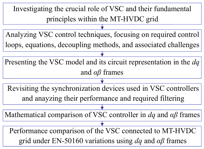
Therefore, the sequential research steps of the paper are depicted in Figure 1. To elaborate on the contributions and the research steps, the paper is structured as follows: Section 2 discusses the fundamentals of the VSC controller and examines the roles of various types of converters within the power grid. Section 3 provides an in-depth analysis of the VSC control technique within the dq frame, while Section 4 presents its counterpart representation in the αβ frame. Section 5 delves into the benefits and limitations of various types of PLLs and FLLs, analyzing their performance under varying frequency conditions. Also, Section 6 outlines a comprehensive comparison between the SRF and STRF. Section 7 presents the simulation results that validate the control techniques discussed. Finally, Section 8 offers conclusions drawn from the analysis and presents findings.

2. Fundamentals of the VSC Controller

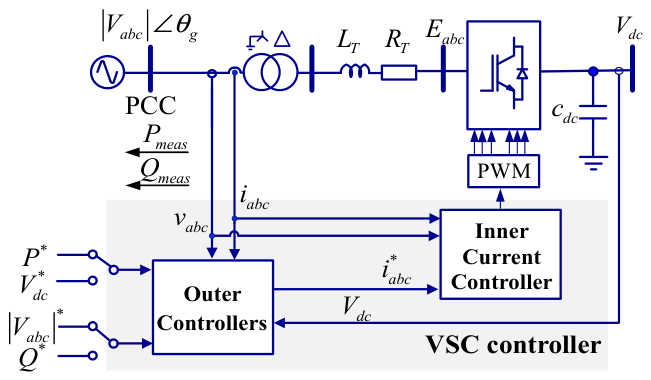
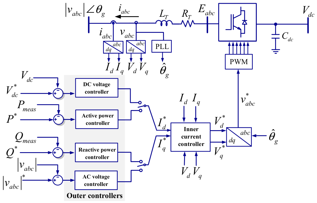
The VSC controller is designed using cascaded control loops. As illustrated in Figure 2, a typical three-phase VSC can be used to connect HVDC networks to the conventional AC electrical power grid, in which $P^{\ast }$ and $Q^{\ast }$ represent the reference values for active and reactive power, respectively, while $P_{meas}$ and $Q_{meas}$ denote the corresponding measured values. Also, ${\left|V_{abc}\right|}^{\ast }$ and $V_{dc}^{\ast }$ represent the references for the AC and DC voltages, respectively. Moreover, $C_{dc}$ is the DC link capacitor, $L_T$ is the total (equivalent) Thévenin of the filter, and the transformer’s leakage inductance, while $R_T$ is the lumped AC-side resistance seen by the converter, including transformer winding resistance, filter resistance, and any short line resistance.

The network of Figure 2 consists of a center-tapped DC voltage source that supplies a switched three-phase bridge converter, an output filter, and the VSC controller. Indeed, the VSC outputs interface with the utility grid through a filter located after the VSC. Moreover, the VSC controller comprises an inner current controller (ICC) integrated with multiple outer controllers (OC). The ICC functions as a high-speed dynamic control loop tasked with regulating AC currents, utilizing reference signals derived from external control loops. Various control strategies can be employed in the ICC [18,19], but in general, they have the same bandwidth design principles, in which [20]

• The ICC bandwidth ($f_{c, ICC}$) is engineered to be fast for overcurrent protection, restricted primarily by digital delays and switching frequencies ($f_{ICC}<f_{SW}/10$).
• The outer loops ($f_{c, outer}$) are systematically designed to be at least 5 to 10 times slower than the ICC ($f_{c, outer}<f_{c, ICC}/10$) to ensure dynamic decoupling, enabling the simplification of the inner loop as a unity-gain element during outer loop tuning.

However, ICC strategies are still insufficient for operation under unbalanced voltage conditions, which can occur due to unbalanced loading on the grid or as a result of unbalanced fault situations. When a VSC connected to the HVDC grid interfaces with an AC grid exhibiting these unbalanced voltages, it is necessary to regulate both positive and negative current sequences accurately. It is noted that such an unbalanced voltage can induce power flow oscillations at twice the fundamental frequency. Therefore, the implementation of sequence current control not only helps to mitigate these power ripples but also proves to be effective in achieving voltage compensation and balancing within the grid [21,22,23].

A common strategy to control unbalanced current sequences is to use a double SRF (DSRF) with a PI regulator, where positive and negative sequence currents are decoupled [24]. In this method, the positive sequence reference frame (PSRF) is responsible for regulating the positive sequence component of current, and the negative sequence reference frame (NSRF) manages the negative sequence component. Each frame contains only DC components due to the decoupling of current sequences. Still, the relatively complex procedure for extracting these sequence elements can limit its application to scenarios that necessitate a fast transient response. On the other hand, it is feasible to control the sequence components without the need for current sequence extraction by implementing the current controller in an STRF with PR controllers. Indeed, PR controllers inherently manage harmonic and sequence components by targeting specific frequencies (e.g., ${\omega }_e$ for the positive sequence, $-{\omega }_e$ for the negative sequence). Therefore, the double fundamental frequency effect no longer exists [25,26,27]. Another advantage of implementing the ICC in an STRF is that the decoupling technique, required for the inner loop in the dq frame, is no longer necessary in the $\alpha \beta$ frame.

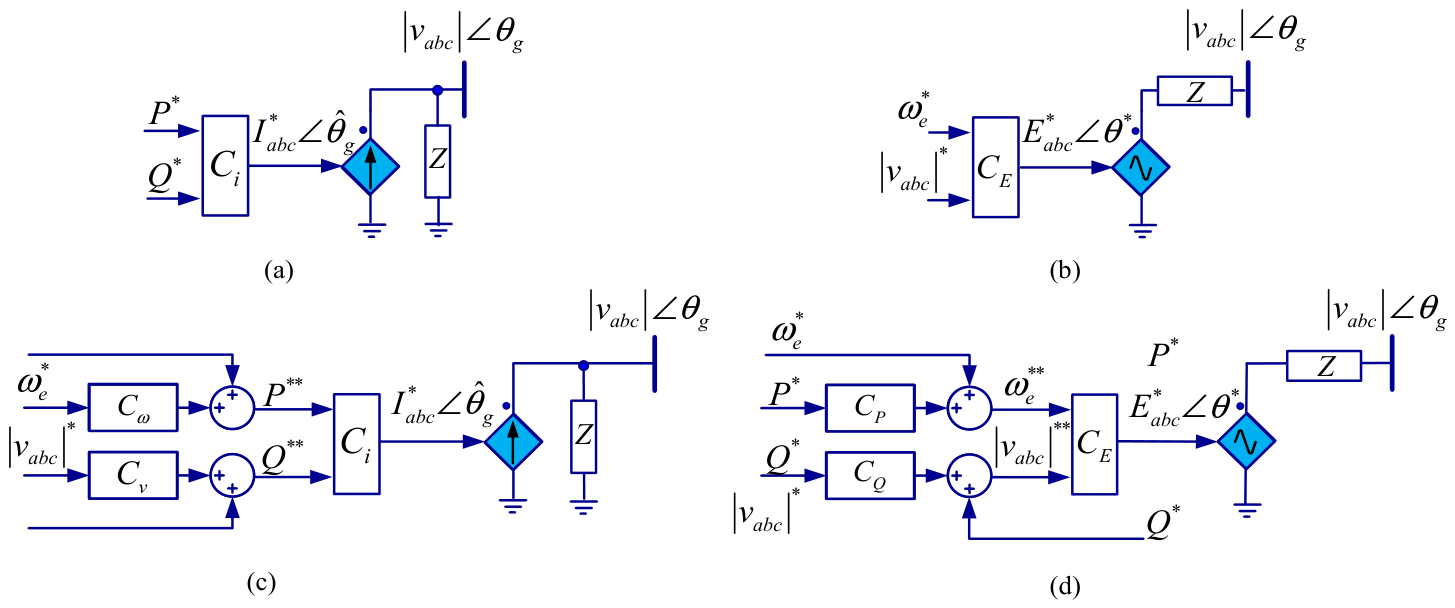
The functionality of the controller is determined by the specific source type of the VSC that it aims to replicate in its interaction with the power system. Specifically, it operates as a voltage controller when functioning as a “voltage source” and as a “current controller” when emulating a current source. As illustrated in Figure 3, depending on the operational context of the VSC within an AC network, it can be categorized into grid-feeding, grid-supporting, and grid-forming types. In Figure 3, $C_i$ and $C_E$ denote the current and voltage control loops, respectively. $C_{\omega }$ and $C_v$ refer to the control loops for angular frequency and AC voltage amplitude. Also, $C_P$ and $C_Q$ represent the control loops for active and reactive power, respectively. Furthermore, ${\widehat{\theta }}_g$ represents the phase angle estimated by the PLL, while ${\theta }^{\ast }$ denotes the phase angle generated through grid-forming techniques.

For a grid-supporting converter functioning as a voltage source, the influence of link impedance is typically incorporated within the internal control loop to effectively emulate the desired source characteristics [28,29,30]. Grid-feeding converters operate by injecting controllable currents with a defined phase angle relative to the AC grid voltage, requiring continuous monitoring of the AC voltage phasor for precise control [31]. The controller’s outer loops play an important role in modulating the output current to meet specific active and reactive power demands. In contrast, grid-forming converters are essentially modeled as voltage sources, functioning to stabilize frequency and voltage within pre-determined limits. One of the main objectives of a grid-forming converter is to emulate the characteristics of conventional synchronous generators by delivering virtual inertia and damping that is essential for stabilizing weak AC grids [32]. In current-source-based grid-supporting configurations, the primary focus shifts to the regulation of both active and reactive power. Meanwhile, voltage source grid-supporting systems concentrate on the primary control of AC voltage and frequency.

Figure 3 shows that in grid-feeding and current-source-based grid-supporting configurations, the VSC relies on the grid’s phase angle for synchronization. Conversely, in the grid-forming architectures and voltage-source-based grid-supporting setups, the VSC itself generates the phase angle. This distinction allows the VSC to exert control over the phase angle at the PCC, enabling operation in an islanded mode. In the current source model, however, real-time phase angle measurements are essential. Typically, this phase angle is supplied by a PLL or an FLL, depending on the chosen control strategy for the VSC. When utilizing an SRF for VSC control, accurate measurement of the PCC’s phase angle is needed, while during operation in the $\alpha \beta$ frame, precise determination of the grid’s angular frequency is crucial for the effective operation of the PR controller. This frequency measurement is done by an FLL. To delve deeper into the nuances of each framework, the subsequent sections provide a detailed exploration of these reference frames.

3. Synchronous Reference Frame

The PI controllers are well-regarded for their effectiveness in DC applications, achieving zero steady-state error due to the integral action. In DC systems (0 Hz), a PI controller exhibits infinite gain, enabling precise control; however, when applied to AC systems, it cannot completely mitigate steady-state errors with the sinusoidal inputs. Specifically, PI controllers demonstrate a delayed tracking response, and it becomes impractical to set the gains sufficiently high to eliminate these errors. To address this limitation, a common technique is to transform AC signals into DC components.

This conversion effectively transfers balanced sinusoidal waveforms, typically at grid frequencies such as 50 or 60 Hz, into constant (DC) values within the rotating dq frame, contingent on aligning the rotating frame with the grid voltage phase. Consequently, this process shifts the control paradigm from the AC to the DC domain, which is notably advantageous for PI controllers. By transforming sinusoidal error signals into DC equivalents, the PI controller can regulate AC signals as though they were DC, effectively extending its infinite gain characteristics to the desired AC frequency. This methodology significantly improves the precision of the PWM controller, making current regulation in the SRF a prevalent strategy for current control. Furthermore, these controllers are capable of providing a rapid response and can automatically compensate for any dead-time effects, with performance enhancements easily achievable through the implementation of an anti-windup mechanism [33]. Since the control architecture operates in the synchronous dq frame, it necessitates continuous access to the grid phase angle for synchronization, which is typically provided by a PLL. The primary goal of the PLL is to synchronize the voltage-controlled oscillator (VCO) in frequency and phase with the input signal during the locking condition.

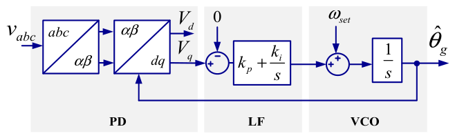
A standard PLL configuration consists of a phase detector (PD), a loop filter (LF), and a VCO, as depicted in Figure 4. In essence, the PLL evaluates the quadrature axis (q-axis) of the grid voltage, $V_q$, aiming to maintain it at zero [34]. Indeed, $V_q$ quantifies the phase discrepancies between the actual grid voltage phase and the phase estimation derived from the PLL algorithm.

This adjustment in phase angle is achieved through a conventional PI regulator inside the LPF that meets the desired lock condition. The conventional PLLs utilize a PI controller in their LF. In contrast, employing a PID controller can enhance dynamic performance [35]. However, this enhancement can pose challenges in the tuning process.

The estimated phase angle of the PLL, i.e., ${\widehat{\theta }}_g$, is used to transform the ICC control parameters from abc to dq frame. This transition usually involves a two-step procedure that incorporates the Clarke and Park transformations [36]. In the first step, the Clarke transformation projects the three-phase abc quantities onto a two-axis stationary reference frame ($\alpha \beta$), thereby simplifying the system dynamics to two dimensions while retaining the critical dynamic characteristics of the original three-phase system. The mathematical representation of the power-invariant Clark transform can be expressed as follows [37]:

$$\left[\begin{array}{l}{x}_{\alpha }\\ x_{\beta }\end{array}\right]=\sqrt{{\displaystyle \frac{2}{3}}}\left[\begin{array}{ccc}\begin{array}{l}1\\ 0\end{array}& \begin{array}{l}-{\displaystyle \frac{1}{2}}\\ {\displaystyle \frac{\sqrt{3}}{2}}\end{array}& \begin{array}{l}-{\displaystyle \frac{1}{2}}\\ -{\displaystyle \frac{\sqrt{3}}{2}}\end{array}\end{array}\right]\left[\begin{array}{c}{x}_a\\ x_b\\ x_c\end{array}\right]$$

(1)

where x can represent current, voltage, or any specific variable of interest, and $x_{\alpha \beta }$ are the corresponding components of the three-phase variable, i.e., $x_{abc}$, transformed into the $\alpha \beta$ reference frame. The Clarke transformation in (1) maps the three-phase abc quantities onto the orthogonal stationary αβ frame; the factor $\sqrt{2/3}$ ensures power invariance. This reduced two-axis form applies to three-phase three-wire systems, where the absence of a neutral return gives $x_a+x_b+x_c=0$, so the zero-sequence component vanishes and is omitted.

In the subsequent step, the Park transformation aligns the $\alpha \beta$ components into a rotating reference frame (dq) that is synchronized with the grid voltage phase angle (${\theta }_g$). The PLL is commonly employed to accurately estimate this phase angle. The Park transformation equation is expressed as follows:

$$\left[\begin{array}{l}{x}_d\\ x_q\end{array}\right]=\left[\begin{array}{cc}\cos (\theta )& \sin (\theta )\\ -\sin (\theta )& \cos (\theta )\end{array}\right]\left[\begin{array}{l}{x}_{\alpha }\\ x_{\beta }\end{array}\right]$$

(2)

where $x_{dq}$ are the dq components of the presented variable. In (2), an orthogonal rotation by the grid angle ${\theta }_g$ aligns the αβ components with the rotating dq frame. Since it is a pure rotation, it preserves the norm and introduces no scaling or distortion. Both transformations are exact linear mappings and add no non-linearity; the non-linear effect relevant to control arises from dependence on the estimated angle ${\widehat{\theta }}_g$, where PLL misalignment produces dq cross-coupling, as analyzed in Section 3 and Section 5. Also, to bypass the intermediate $\alpha \beta$ frame and directly transform three-phase variables into the rotating dq frame, the following equation can be utilized, which combines the Clark and Park transformations [37].

$$\left[\begin{array}{l}{x}_d\\ x_q\end{array}\right]=\sqrt{{\displaystyle \frac{2}{3}}}\left[\begin{array}{ccc}\cos (\theta )& \cos (\theta -{\displaystyle \frac{2\pi }{3}})& \cos (\theta +{\displaystyle \frac{2\pi }{3}})\\ -\sin (\theta )& -\sin (\theta -{\displaystyle \frac{2\pi }{3}})& -\sin (\theta +{\displaystyle \frac{2\pi }{3}})\end{array}\right]\left[\begin{array}{c}{x}_a\\ x_b\\ x_c\end{array}\right]$$

(3)

This transformation is widely used in control systems. Figure 5 shows the structure of a VSC control system based on the presented theory. As shown in the figure, the converter operation is governed by measuring the grid voltage and current, then transforming them from the abc to the dq reference frame. The gathered dq components are utilized within the ICC. Also, a higher-level control loop is employed that determines the necessary d- and q-axis current components for this inner current controller. By orienting the d-axis with the grid voltage vector, control strategies can effectively decouple the management of active and reactive power components.

The VSC controller is responsible for regulating the active and reactive power injected into the grid through a closed-loop current regulator that commands a high-frequency PWM switching block. The target active and reactive power commands, i.e., $P^{\ast }$ and $Q^{\ast }$, are either received from a remote controller or set to fixed values to achieve the desired level of active and reactive power. As illustrated in Figure 5, the currents, $i_{abc}$, and the voltages, $v_{abc}$, are measured in the abc reference frame and subsequently transformed into SRF using (3). These measurements are then used to calculate the measured active and reactive power, i.e., $P_{meas}$, and $Q_{meas}$, by using

$$\left\{\begin{array}{c}{P}_{meas}=V_d{I}_d+V_q{I}_q\\ Q_{meas}=V_q{I}_d+V_d{I}_q\end{array}\right.$$

(4)

where $V_{dq}$ and $I_{dq}$ represent the measured grid voltages and currents in the dq reference frame. Under seamless alignment ($v_q\equiv 0$), which is achieved by the PLL, these power equations are reduced to $P_{meas}=V_d{I}_d$ and $Q_{meas}=V_d{I}_q$. The calculated power values are subsequently compared to their reference targets. The resulting power errors are processed through standard PI controllers, which generate the commanded values for the current regulators at the subsequent control level. The current controllers using the dq frame employ PI regulators with stable gains, which are tuned using either conventional methods [19] or metaheuristic approaches [38,39].

This setup facilitates the precise injection of specified levels of active and reactive power, based on the measured voltages and currents from the grid. The current control loop generates desired average output voltages for each phase leg, which are then processed through the PWM to produce the corresponding phase leg switching commands. This transformation enables the use of a simple PI structure for both the inner and outer control loops. Since these loops operate with direct current (DC) variables in the SRF, they can achieve zero steady-state error due to the infinite DC gain inherent in a PI regulator [40,41]. Furthermore, only two regulator structures are necessary, specifically in the d and q axes. This is due to the floating neutral connection of the utility grid, which ensures that the three-phase currents always sum to zero, resulting in no zero-sequence current flowing through the inverter system.

The corresponding equation of the VSC in dq reference can be calculated by considering the voltage drop across $L_T$ and $R_T$ as

$$\begin{array}{l}{L}_T{\displaystyle \frac{d}{dt}}\left[\begin{array}{c}{I}_d\\ I_q\end{array}\right]+R_T\left[\begin{array}{c}{I}_d\\ I_q\end{array}\right]+\left[\begin{array}{cc}0& -L_T{\omega }_e\\ L_T{\omega }_e& 0\end{array}\right]\left[\begin{array}{c}{I}_d\\ I_q\end{array}\right]=\Delta V_{drop},\\ \Delta V_{drop}=\left[\begin{array}{c}{E}_d\\ E_q\end{array}\right]-\left[\begin{array}{c}{V}_d\\ V_q\end{array}\right]\end{array}$$

(5)

in which $\Delta V_{drop}$ is the voltage drop across the $L_T$ and $R_T$ and $\left[\begin{array}{cc}0& -L_T{\omega }_e\\ L_T{\omega }_e& 0\end{array}\right]\left[\begin{array}{c}{I}_d\\ I_q\end{array}\right]$ is the cross-coupling effect. Therefore, (5) can be rewritten as

$${\displaystyle \frac{d}{dt}}\left[\begin{array}{c}{I}_d\\ I_q\end{array}\right]=\left[\begin{array}{cc}-{\displaystyle \frac{R_T}{L_T}}& {\omega }_e\\ -{\omega }_e& -{\displaystyle \frac{R_T}{L_T}}\end{array}\right]\left[\begin{array}{c}{I}_d\\ I_q\end{array}\right]+{\displaystyle \frac{1}{L_T}}\left(\left[\begin{array}{c}{E}_d\\ E_q\end{array}\right]-\left[\begin{array}{c}{V}_d\\ V_q\end{array}\right]\right)$$

(6)

Equations (5) and (6) are obtained by applying Kirchhoff’s voltage law across the AC-side phase reactor ($L_T$, $R_T$) and transforming the resulting abc equations into the dq frame. Because the dq frame rotates at ${\omega }_e$, the time derivative of the rotating unit vectors introduces the speed–voltage terms $+{\omega }_e{L}_T{I}_q$ and $-{\omega }_e{L}_T{I}_d$, which constitute the inherent cross-coupling between the two axes.

By considering the modulation indexes as

$$\left[\begin{array}{l}{M}_d\\ M_q\end{array}\right]=[{\mathrm{T}}_{abc/dq}]\left[\begin{array}{l}{m}_a\\ m_b\\ m_c\end{array}\right]$$

(7)

and analyzing the voltage transformation between the DC and AC domains of the VSC via modulation techniques, the following equations for the average model of the VSC are derived:

$$E_d=M_d{V}_{dc},E_q=M_q{V}_{dc}$$

(8)

in which $M_d$ and $M_q$ represent the modulation indices in the dq frame, highlighting their critical role in scaling the DC voltage ($V_{dc}$) to derive the necessary AC voltage components.

Equations (7) and (8) express the converter AC voltages in terms of the dq modulation indices using the average converter model, in which the switching action is represented by its fundamental-frequency average and the high-frequency PWM harmonics are neglected.

Let ${i^{\prime }}_{dc}$ represent the input current to the VSC. By considering (8) and acknowledging the equivalence between the input active power ($P_{d{c}_{in}})$ and the output active power of the VSC ($P_{a{c}_{out}})$, in light of the average model assumption, the following equation is derived:

$$\begin{array}{l}{V}_{dc}{i^{\prime }}_{dc}=P_{d{c}_{in}}=P_{a{c}_{out}}=E_d{I}_d+E_q{I}_q,\\ V_{dc}{i^{\prime }}_{dc}=V_{dc}(M_d{I}_d+M_q{I}_q),\\ {i^{\prime }}_{dc}=M_d{I}_d+M_q{I}_q\end{array}$$

(9)

in which $P_{d{c}_{in}}$ and $P_{a{c}_{out}}$ are the input active power from the DC side and the output AC active power from the VSC, respectively. This equation is obtained from instantaneous power balance between the DC and AC sides ($V_{dc}{i}_{dc}^{\prime }=E_d{I}_d+E_q{I}_q$), assuming a lossless converter, which combined with (6)–(8) yields the complete dq model within the dq frame that can be rewritten as follows:

$$\left\{\begin{array}{c}{V}_d=M_d{V}_{dc}-R_T{I}_d-L_T{\displaystyle \frac{\mathrm{d}{I}_d}{\mathrm{d}t}}+{\omega }_e{L}_T{I}_q\\ V_q=M_q{V}_{dc}-R_T{I}_q-L_T{\displaystyle \frac{\mathrm{d}{I}_q}{\mathrm{d}t}}-{\omega }_e{L}_T{I}_d\end{array}\right.$$

(10)

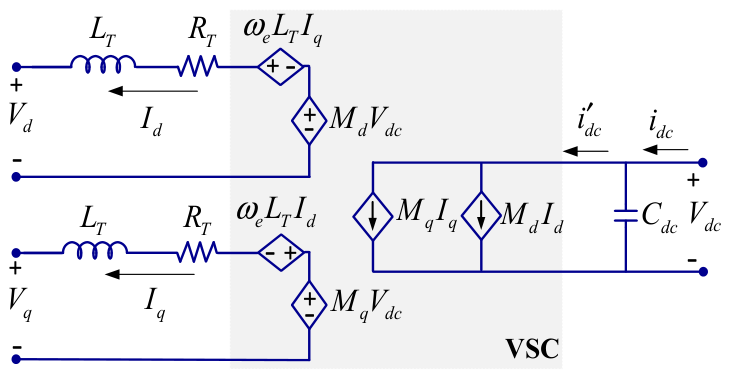
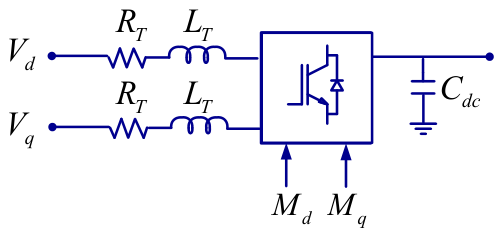
Therefore, the equivalent circuit representations of the VSC in the SRF are illustrated in Figure 6, whereas its corresponding model representation is depicted in Figure 7.

Equation (10) and Figure 6 indicate that the dynamic model in the dq frame introduces cross-coupling between the d-axis and q-axis currents, attributable to the rotational transformation. Specifically, the coupling terms, which are dependent on the angular velocity ${\omega }_e$ and inductance $L_T$, manifest as ${\omega }_e{L}_T{I}_q$ in the d-axis voltage equation and $-{\omega }_e{L}_T{I}_d$ in the q-axis voltage equation. 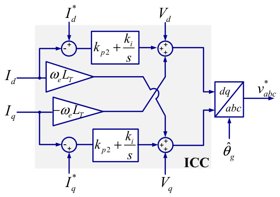These interactions complicate the independent regulation of $I_d$ and $I_q$, resulting in suboptimal dynamic performance. To address this, as shown in Figure 8, a decoupling feedforward strategy is employed within the current control loop. This involves compensating for the cross-coupling effects by subtracting ${\omega }_e{L}_T{I}_q$ from the output of the d-axis PI controller and adding ${\omega }_e{L}_T{I}_d$ to the output of the q-axis PI controller. This strategy effectively linearizes the system dynamics, enabling each current component to be controlled independently by its respective PI controller. Consequently, the decoupling approach enhances control precision and improves transient response characteristics.

It should be noted that the effectiveness of this feedforward decoupling depends directly on the accuracy of the assumed parameters, namely the total inductance $L_T$ and the estimated angular frequency ${\omega }_e$. Since the compensating terms are proportional to ${\omega }_e{L}_T$, any mismatch between the assumed and actual inductance, or any error in the estimated frequency provided by the PLL, leaves a residual cross-coupling between the $d$- and $q$-axis currents that must be rejected by the PI controllers. In practical HVDC applications, the grid equivalent inductance varies with the operating condition, so exact decoupling cannot be guaranteed at all times, and the residual coupling grows with the degree of mismatch and with the operating frequency. This dependence is a notable practical drawback of the dq frame; by contrast, as shown later in Section 4, the $\alpha \beta$ frame requires no such decoupling network and is consequently unaffected by inductance mismatch in this respect.

The output commands from the ICC are converted back to the stationary abc reference frame using the phase angle generated by the PLL (${\widehat{\theta }}_e$). These commands are then utilized within an asymmetrical, regular-sampled PWM modulator system to manage the switching actions of each phase leg effectively. Simulating the control systems in this way delivers a highly precise representation of actual physical VSC behavior. This technique is particularly effective in capturing the high-frequency dynamics and filter responses characteristic of these systems.

The Inductive–Capacitive–Inductive (LCL) filters are among the most widely used filters for grid-connected applications. They provide significantly enhanced attenuation of PWM switching harmonics with reduced size and weight compared to conventional inductive (L) filters [37,39,42]. However, these filters can introduce a resonance peak in the plant’s frequency response, potentially leading to resonant stability issues. To mitigate this instability, either passive or active damping within the current regulator is typically necessary [37]. While passive damping can increase system losses, active damping, which incorporates a compensation term proportional to the capacitor current, is generally the preferred method.

4. Stationary Reference Frame

Implemented in an STRF just using (1). The implementation of PR controllers in an $\alpha \beta$ frame offers a distinct advantage over PI controllers operating in a dq frame, particularly for the regulation of unbalanced sinusoidal currents. Unlike PI controllers, PR controllers eliminate the need for decoupling networks and independent sequence control strategies, as they are capable of effectively managing both positive and negative sequence components simultaneously within a single PR block [2].

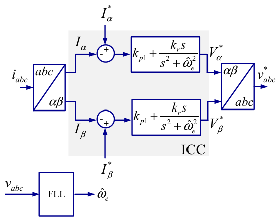
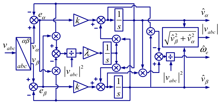
Also, the PR controller in the stationary frame offers infinite gain at both $\pm {\omega }_e$ frequencies. Figure 9 illustrates the current control loop in the $\alpha \beta$ frame in detail, where substituting ${\omega }_e$ with s in the integral part results in an infinite denominator, which enables the controller to achieve zero steady-state error at $\pm {\omega }_e$ angular frequencies. The estimation of the angular frequency of the grid is performed through an FLL. The FLL is a dedicated system designed for precise tracking and locking onto the frequency of an input signal by minimizing the frequency error through a feedback mechanism. It can autonomously estimate and monitor frequency using techniques such as error minimization informed by the input signal’s characteristics, including zero-crossing detection and phase difference analysis [43]. This advanced control solution is extensively applied in power electronics for synchronization and enables enhanced frequency estimation accuracy. The configuration of a three-phase FLL is illustrated in Figure 10, in which ${\widehat{\omega }}_{FLL}$ is the estimated angular frequency of the grid and ${\widehat{v}}_{\alpha }$ and ${\widehat{v}}_{\beta }$ are the filtered grid voltages in the $\alpha \beta$ frame. Also, $k$ and $\lambda$ are tuning parameters.

It should be noted that the FLL can be further optimized using harmonic filtering techniques, such as Cascaded Delayed Signal Cancellation blocks. This implementation enhances precision and ensures that the output remains reliable for reference generation within the VSC [44].

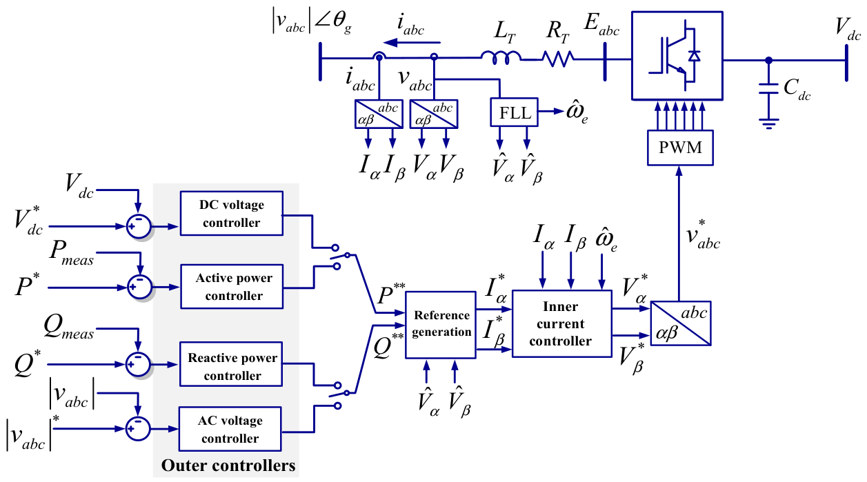
The general control structure of a VSC station that incorporates FLL and PR in the STRF is illustrated in Figure 11. In this configuration, the instantaneous active and reactive powers in the STRF are measured by

$$\left\{\begin{array}{c}{P}_{meas}=V_{\alpha }{I}_{\alpha }+V_{\beta }{I}_{\beta }\\ Q_{meas}=V_{\beta }{I}_{\alpha }-V_{\alpha }{I}_{\beta }\end{array}\right.$$

(11)

then, after comparing these measured signals with their references using the traditional PI controllers, the desired current references in $\alpha \beta$ frame are generated by

$$\begin{array}{l}{I}_{\alpha }^{\ast }={\displaystyle \frac{P^{\ast \ast }{\widehat{V}}_{\alpha }-Q^{\ast \ast }{\widehat{V}}_{\beta }}{{{\widehat{V}}_{\alpha }}^2+{{\widehat{V}}_{\beta }}^2}},\\ I_{\beta }^{\ast }={\displaystyle \frac{P^{\ast \ast }{\widehat{V}}_{\beta }+Q^{\ast \ast }{\widehat{V}}_{\alpha }}{{{\widehat{V}}_{\alpha }}^2+{{\widehat{V}}_{\beta }}^2}}\end{array}$$

(12)

Afterwards, the PR controllers are utilized within the ICC framework to control the VSC’s currents and ensure that steady-state error is effectively eliminated. As illustrated in Figure 10 and Figure 11, the implementation of the controller within the $\alpha \beta$ frame exhibits a more intricate architecture compared to the controller operating in the dq frame. This complexity translates into a greater demand for meticulous parameter tuning and optimization. To facilitate the VSC representation in the $\alpha \beta$ frame, the following steps are conducted in this paper. By considering the average model of the power converter, the next relation is established.

$$V_{dc}{i^{\prime }}_{dc}=P_{d{c}_{in}}=P_{a{c}_{out}}=E_{\alpha }{I}_{\alpha }+E_{\beta }{I}_{\beta }$$

(13)

As the modulation indices within the $\alpha \beta$ frame are

$$\left[\begin{array}{l}{M}_{\alpha }\\ M_{\beta }\end{array}\right]=[{\mathrm{T}}_{abc/\alpha \beta }]\left[\begin{array}{l}{m}_a\\ m_b\\ m_c\end{array}\right]$$

(14)

Then, the terms $E_{\alpha }=M_{\alpha }{V}_{dc}$ and $E_{\beta }=M_{\beta }{V}_{dc}$ are obtained. By substituting them into (13), the following equation is obtained.

$$\begin{array}{l}{V}_{dc}{i^{\prime }}_{dc}=V_{dc}(M_{\alpha }{i}_{\alpha }+M_{\beta }{i}_{\beta }),\\ {i^{\prime }}_{dc}=M_{\alpha }{i}_{\alpha }+M_{\beta }{i}_{\beta }\end{array}$$

(15)

Furthermore, the voltages in the $\alpha \beta$ frame can be written as

$$\left\{\begin{array}{c}{V}_{\alpha }=M_{\alpha }{V}_{dc}-R_T{I}_{\alpha }-L_T{\displaystyle \frac{\mathrm{d}{I}_{\alpha }}{\mathrm{d}t}}\\ V_{\beta }=M_{\beta }{V}_{dc}-R_T{I}_{\beta }-L_T{\displaystyle \frac{\mathrm{d}{I}_{\beta }}{\mathrm{d}t}}\end{array}\right.,$$

(16)

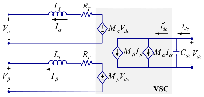
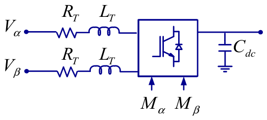
Therefore, the circuit representation of the VSC in the $\alpha \beta$ reference frame is depicted in Figure 12. Also, the model representation of the VSC from the voltage perspective is presented in Figure 13. According to Figure 12, it is evident that there is an absence of current coupling terms, contrasting with the dq representation of the VSC circuit, where such terms are present. Therefore, the ICC in STRF does not require the decoupling technique. However, both controllers’ performance is significantly influenced by their synchronization devices. Therefore, the next section will thoroughly evaluate the various synchronizers employed in both $\alpha \beta$ and dq frame controllers.

5. Analyzing the PLL and FLL Performances

VSC dynamic behavior depends on the inner and outer control loops’ parameters as well as the PLL and FLL dynamics. Under ideal synchronization in the dq frame (i.e., via a high-bandwidth PLL), active and reactive power channels appear as DC signals. This allows the use of simple PI controllers with clear bandwidth separation and minimal cross-coupling in the steady-state condition. Any PLL lag or grid frequency drift reintroduces coupling into the dq signals, shrinking effective active and reactive power control and potentially destabilizing fast loops if not properly compensated. Indeed, phase tracking is sensitive to sags, frequency jumps, and unbalanced conditions. During such disturbances, PLL misalignment injects significant errors into current control loops. But, in $\alpha \beta$ frame controllers, an FLL with high bandwidth is generally employed to estimate the fundamental frequency of the grid voltage. Since the FLL estimates frequency instead of phase, it remains functional under voltage unbalance or distortion [40].

The PLLs are typically categorized into Type-1, Type-2, and Type-3 based on their integral components. Type-1 PLLs tend to display a lower precision level due to the singular gain element within the LF, which results in a steady-state phase error when faced with step frequency changes [45]. To address this limitation, Type-2 PLLs incorporate two integral elements, one within the LF and another in the VCO. This configuration, combined with a zero-pole adjustment, allows the PLL to attain zero steady-state error, benefiting from infinite DC gain at the origin.

Type-3 PLLs enhance this further by integrating a third integral component in the auxiliary frequency detector, enabling improved tracking of frequency ramps. However, a notable drawback of Type-3 PLLs is their increased oscillatory behavior during large transients compared to Type-2 PLLs, which provides a more stable response [46]. It is also crucial to point out that while FLLs excel in transient response, this advantage correlates with diminished phase estimation accuracy in steady-state conditions. This arises from the inherent difference where the FLL locks on frequency, whereas the PLL relies on a phase feedback loop. This approach enhances FLL dynamic response and increases its robustness against DC offset, harmonic distortion, and phase angle jump. The FLL achieves this by monitoring the error between the input signal and the filtered output, using this information to update the estimated frequency through a feedback law. Its real-time tracking capabilities and strong resilience to signal disturbances make the FLL particularly well-suited for synchronization applications in weak AC grids. However, implementing FLL and its filtering techniques is more complex than a conventional PLL.

The PLL and FLL performances can be improved using filters. Moving Average Filter and DSC are conventional filtering techniques employed in PLL and FLL, respectively, to enhance the precision of estimations [44,47]. The MAF equation in Laplace form, which is implemented in the PLL, can be expressed as follows:

$$G_{MF}(s)={\displaystyle \frac{1-e^{-T_{w}s}}{T_{w}s}}$$

(17)

in which ${\tilde{V}}_q$ is the average value of the error signal inside the PLL, and $T_w$ is a specified time window typically aligned with the fundamental period of the input signal ($T$). Also, the DSC equation in Laplace form that is utilized in the FLL is as follows:

$$G_{DSC}(s)={\displaystyle \frac{1+e^{-\frac{Ts}{n_k}}}{2}}$$

(18)

in which $T$ is the fundamental period, and $n$ is the operator delay factor. For proper filtering in FLL, typically two cascaded DSCs with operator delay factors of $n_1=4$ and $n_2=24$ are recommended that allow the effective suppression of typical harmonic orders present in the grid, specifically at $h=-5$ and $h=+7$. The selection of the filtering parameters follows the established design guidelines reported in [43,44,45,46], and is intended to provide standard, reproducible synchronization performance rather than application-specific optimization. For the MAF used in the PLL, the averaging window $T_w$ is set equal to the fundamental period $T$ of the grid voltage, which fully attenuates the dominant even-order and ripple components at the cost of a settling time on the order of one fundamental cycle, thereby trading bandwidth for steady-state accuracy.

To evaluate the performance of the PLL and FLL under conditions of frequency jumps, this study conducts a comparative analysis focused on their respective responses. The tuning parameters for both systems were selected in accordance with the values presented in [44,46]. In this regard, the gains are defined as $k=160$ and $\lambda =12791$ for the FLL. Also, in the case of the Type-2 PLL, the proportional and integral gains are configured at $k_p=114$ and $k_i=6634$, respectively. This configuration is specifically chosen to attain a damping ratio of 0.707, ensuring optimal stability and transient response of the PLL system.

It should be noted that the subsequent comparison is drawn between the two complete synchronization schemes as practically implemented, the PLL with its Moving Average Filter (PLL+MAF) and the FLL with its cascaded DSC (FLL+DSC), rather than between the bare PLL and FLL cores, since in practice neither synchronizer operates without its associated filtering, and each filter is the standard choice for its respective scheme.

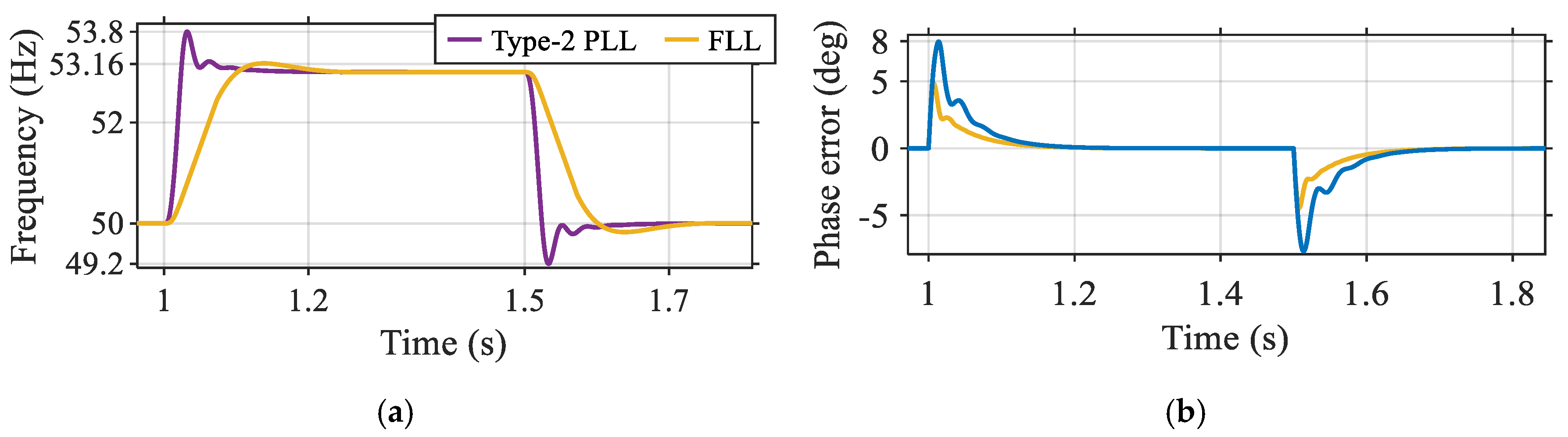
The comparison is performed using MATLAB Simulink with a discrete solver operating at 0.1-millisecond time intervals. Figure 14 illustrates the performance of the FLL and PLL in response to a 3 Hz frequency jump. It is important to note that such abrupt changes are not typically encountered in real-world grid scenarios; this analysis is conducted purely to evaluate the controllers’ performance under critical conditions. To provide a reliable assessment, a three-phase sinusoidal signal generator with a predetermined frequency and phase angle is employed to analyze the phase and frequency tracking capabilities of each controller during the frequency jump. This figure isolates the synchronizers’ own input-to-output response to a standard frequency-step test signal, whereas the subsequent case studies (in the Simulation Results Section) show the disturbance and transient responses of the complete VSC, in which the PLL and FLL act as embedded components influencing the overall control behavior. In Figure 14a, the FLL demonstrates an overshoot of 0.16 Hz, whereas the PLL exhibits a more pronounced overshoot of 0.8 Hz for the same frequency step change. Furthermore, Figure 14b illustrates that under this condition, the PLL’s estimated phase angle error reaches 8 degrees, which may jeopardize the stability of the power converter. In contrast, the FLL maintains a phase angle error of 5 degrees. This comparison underscores the superior robustness of the FLL against frequency variations relative to the PLL.

6. Comparison Between Synchronous and Stationary Reference Frames

In this section, we will explore both the STRF and SRF in depth. It is essential to note that the proper functioning of the $\alpha \beta$ frame controller is affected by the FLL and the dq frame controller by the PLL, as discussed in the previous section.

A key advantage of the stationary reference frame is the reduced need for conversions between frames, requiring only the Clark transformation. In contrast, the synchronous reference frame necessitates both the Clark and Park transformations for the measurement of voltage and current signals and VSC inner and outer control blocks.

This additional transformation introduces a computational burden in comparison with the stationary reference frame. However, the $\alpha \beta$ frame controller involves its own complexities, including the need for a reference signal generation block and the intricate implementation of the three-phase FLL, making it more challenging to implement compared to the synchronous reference frame. Additionally, the complexity of both controllers is significantly influenced by the filtering techniques employed, which vary based on the application of the VSC and the specific characteristics of the AC grid to which it is connected. In fact, effective VSC control in both reference frames relies heavily on these filtering methods to mitigate the effects of fluctuations. In the dq frame, the impact of harmonics and fluctuations can be reduced through filtering methods, such as employing cascaded notch filtering [48], with relevant equations and further details provided in

Table 1. Comparison between αβ and dq reference frames.

Feature	Stationary Reference Frame ($\mathit{\alpha }\mathit{\beta }$)	Synchronous Reference Frame (dq)
Control Variables	Sinusoidal AC quantities	DC quantities
Controller Type	Outer loop is a PI with the transfer function $G_{PI-outer}(s)=k_{p-outer1}+{\displaystyle \frac{k_{i-outer1}}{s}}$. Inner loop is a PR with the transfer function $G_{PR}(s)=k_{p1}+{\displaystyle \frac{k_{r}s}{s^2+{\omega }_e^2}}$	Both inner and outer loops are PI with the transfer function $G_{PI-outer}(s)=k_{p-outer2}+{\displaystyle \frac{k_{i-outer2}}{s}},G_{PI-inner}(s)=k_{p2}+{\displaystyle \frac{k_{i2}}{s}}$
Transform Required	Clarke only $abc\to \alpha \beta$	Clarke + Park $abc\to \alpha \beta \to dq$
Synchronizing Technique	Requires ${\widehat{\omega }}_e$ and ${\widehat{V}}_{\alpha },{\widehat{V}}_{\beta }$ provided by an FLL	Requires ${\widehat{\theta }}_e$, provided by a PLL
Steady-State Error	Zero. Due to the infinite gain at the grid frequency, $\underset{s\to \pm {\omega }_e}{\lim }\left(k_{p1}+{\displaystyle \frac{k_{r}s}{s^2+{\omega }_e^2}}\right)=\infty$	Zero. Due to the infinite DC gain, $\underset{s\to 0}{\lim }\left(k_{p2}+{\displaystyle \frac{k_i}{s}}\right)=\infty$
Dynamic Response	Potentially faster for specific applications	Moderate, especially for power control, primarily attributed to the Park transform
Computational Complexity	Moderate to high due to the use of the FLL with complex filters, reference generation, and variable resonant frequency	High due to real-time Park/Inverse Park transformations, and a PLL, which increase computational burden
Ease of Implementation	More complex to set up (FLL, PR and instantaneous reference generation)	Less complex to set up
Harmonic Handling	The h harmonic appears on $h{\omega }_e$ frequency Requires parallel resonant terms for the selected harmonics. The open-loop transfer function of the controller is $G_{OC}(s)=k_{p1}+{\displaystyle \sum _{h\in \left\{1,3,5,\dots \right\}}\frac{k_{r,h}s}{s^2+{(h{\omega }_e)}^2}}$	The h harmonic appears on (h − 1)${\omega }_e$ frequency. Requires filtering methods like cascaded notch filters for the targeted harmonics. $G_{notch,h}={\displaystyle \frac{s^2+{\left((h-1){\omega }_e\right)}^2}{s^2+2\zeta (h-1){\omega }_{e}s+{\left((h-1){\omega }_e\right)}^2}}$ Open-loop transfer function of the controller: $G_{oc}(S)=(k_{p2}+{\displaystyle \frac{k_i}{s}})\times G_{notch,h_3}{G}_{notch,h_5}\dots$
Power Control	Robust and direct. Instantaneous measurement of active and reactive powers. Can add a simple LPF for power measurement. $P_{avg}=\underset{{\omega }_f\ll 2{\omega }_e}{LPF\left\{P(t)\right\}},Q_{avg}=\underset{{\omega }_f\ll 2{\omega }_e}{LPF\left\{Q(t)\right\}}$	Moderate and indirect. Averaged values of active and reactive powers, due to the use of the Park transform (requires a PLL). In an ideal condition without disturbance: $P_{avg}=V_d{I}_d,Q_{avg}=V_d{I}_q$
Disturbance Handling	Robust, as directly affected by an FLL with a high bandwidth. The FLL locks in frequency and is more robust against phase jumps and large frequency changes. The estimated frequency by the FLL is ${\widehat{\omega }}_e(t)={\displaystyle \frac{{\widehat{v}}_{\alpha }(t)\frac{d{\widehat{v}}_{\beta }(t)}{dt}-{\widehat{v}}_{\beta }(t)\frac{d{\widehat{v}}_{\alpha }(t)}{dt}}{{\left({\widehat{v}}_{\alpha }(t)\right)}^2+{\left({\widehat{v}}_{\beta }(t)\right)}^2}}$	Moderate, as directly affected by PLL with a narrow bandwidth. The PLL is more accurate than the FLL in small disturbances. The estimated phase angle by the PLL is $\begin{array}{l}{\widehat{\theta }}_g(t)={\displaystyle {\displaystyle \underset{0}{\overset{t}{\int }}}{\omega }_{est}(\tau )d\tau },\\ {\omega }_{est}(t)={\omega }_n+K_{p\_pll}\left(v_q(t)\right)+K_{i\_pll}{\displaystyle {\displaystyle \underset{0}{\overset{t}{\int }}}{v}_q(\tau )d\tau }\end{array}$

. On the other hand, in an $\alpha \beta$ frame controller, harmonic rejection and unbalance handling are accomplished using multiple resonant controllers tuned to specific frequencies [36]. To enhance comprehension of the $\alpha \beta$ and dq frame controllers, and to outline their associated benefits and limitations, Table 1 is provided below. This table focuses on critical issues such as required transformations, harmonic and disturbance handling.

Tuning the αβ and dq Frame Control Parameters

One of the critical issues that affects the performance of the VSC is the proper tuning of the control parameters of the converter’s inner and outer loops. Also, in practical applications, the delay introduced by the controller sampling (one-half the carrier period $\Delta T/2$), transport (roughly another half the carrier period $\Delta T/2$), and processing (usually minimized with optimized DSPs but can be a few microseconds depending on the hardware), must be considered while parameters are tuned. In the real implementation, the total delay ($T_d$) used in the control design is approximately 0.75 of a carrier period, i.e., $T_d=0.75\Delta T$. Moreover, for an ideal PR controller in ICC, the forward gain block, $G_c\left(s\right)$, is represented by (19) [49]:

$$G_c(s)=V_{dc}\left[k_{p1}+{\displaystyle \frac{k_{r}s}{s^2+{\omega }_e^2}}\right]$$

(19)

by considering a desired phase margin (${\varphi }_m$) for the entire controller and the plant, the maximum crossover frequency (${\omega }_{c\left(max\right)}$) is:

$${\omega }_{c(\max )}={\displaystyle \frac{\pi /2-{\varphi }_m}{T_d}}$$

(20)

and the proportional gain of the controller can be roughly calculated as follows.

$$k_{p1}\approx {\displaystyle \frac{{\omega }_{c(\max )}L}{V_{dc}}}$$

(21)

The parameter $k_{p1}$ is related to the maximum crossover frequency, DC voltage, and the plant series inductance (L). Also, the resonant gain can then be calculated as:

$$k_r\approx {\displaystyle \frac{{\omega }_{c(\max )}{k}_{p1}}{10}}$$

(22)

It is worth noting that the analysis presented in [49] clearly demonstrates that the gain optimization process is applicable to all variations of linearized AC current regulators, including PI controllers in dq frames. This assertion is further supported by [50], which delves into the equivalence between PI and PR controllers. Also, [51,52] demonstrate that at least a tenfold bandwidth difference effectively decouples the fast inner current control from the slower outer voltage or power control, thereby enhancing harmonic mitigation and transient response. Therefore, the parameters of PI controllers in outer loops are selected as:

$$k_{p-outer1}\le 0.1k_{p_1},\hspace{1em}{k}_{i-outer1}\le 0.1k_r$$

(23)

It is important to note that Equations (19)–(23) represent standard tuning relationships derived from established methodologies. These relations are utilized here to provide a consistent framework for comparison, ensuring that the αβ and dq frame controllers are evaluated under a fair and reproducible standard. To compare the performance of the studied control techniques, the following section presents the simulation results.

7. Simulation Results

This section presents a comparative analysis of the two control strategies for VSC: one utilizing a PR controller in the $\alpha \beta$ reference frame with an FLL, and the other employing a PI controller in the dq frame with a PLL. The effectiveness of each strategy is inherently linked to the performance of the associated synchronization mechanisms. Consequently, the careful selection of standard synchronizers with well-designed filtering characteristics is crucial for optimizing system performance. 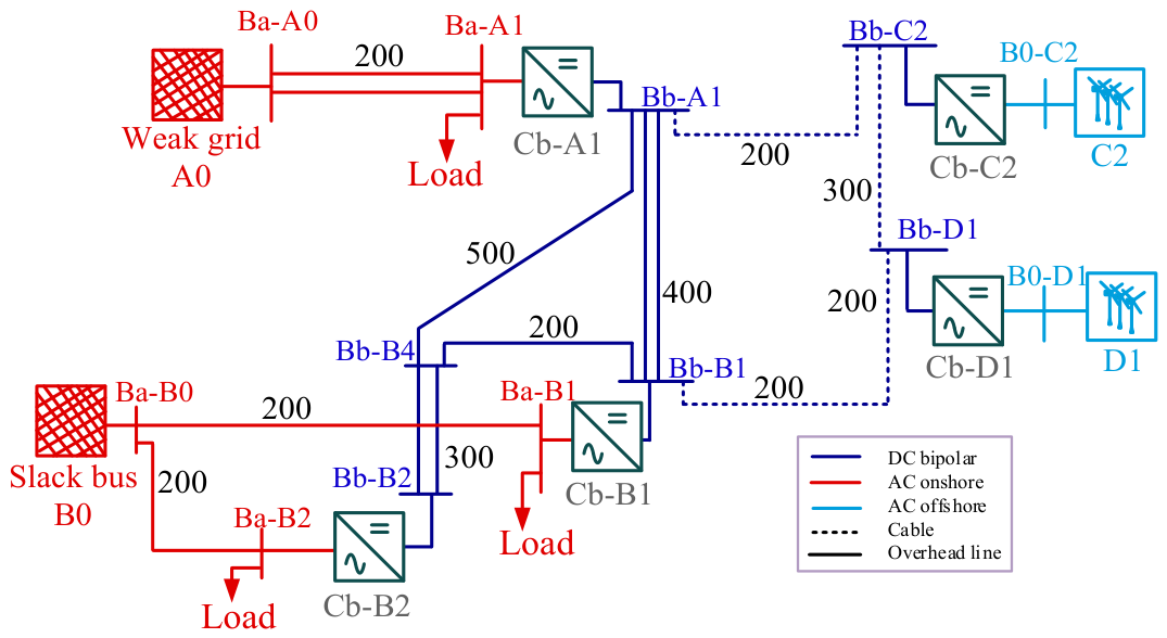Therefore, this paper employs a PLL integrated with MAF, where the time window is set to match the fundamental period of the grid, which is implemented in the dq frame. Additionally, the FLL is utilized with a two-stage DSC mechanism with operator delay factors of 4 and 24. This configuration enables a meaningful and practical comparison of the two control approaches. Also, to ensure a standardized comparison, the Cigre-DCS 3 network is utilized and its configuration is depicted in Figure 15 [53].

The outer loop of the VSC’s active power control operates as a power regulator, utilizing a PI controller. The active power reference is adjusted through a frequency-to-power droop characteristic. Concurrently, the reactive power control loop employs a PI controller in its outer loop to stabilize the AC voltage levels. Additionally, in all simulation case studies, the utilized gains for the PI and PR are summarized in Table 4. It is essential to underscore that the selected gains, including those for the FLL and PLL, as well as the gains for the outer and inner loops of the VSC controllers in both reference frames, have been meticulously tuned following the methodologies presented in the relevant references discussed in prior sections. Moreover, in these simulations, the ICCs depicted in Figure 8 and Figure 9 are employed. Also, the configurations outlined in Figure 5 and Figure 11 are utilized to compare these two control strategies under different grid conditions. The simulations in all case studies are conducted using a discrete fixed-step ODE-3 (Bogacki–Shampine) solver with a sampling interval of 0.1 milliseconds.

This multi-terminal HVDC (MT-HVDC) test grid is a subsystem of the Cigre-B4 network. It has been utilized in this analysis to ensure reliability and provide a fair comparison. Furthermore, the selected scenarios for analyzing each control strategy are assessed within the specified limits of EN-50160 regarding the grid’s variations. Specifically, under normal operating conditions the supply voltage magnitude should remain within ±10% of the nominal value, the voltage unbalance factor (ratio of negative- to positive-sequence voltage) should not exceed 2%, and the total harmonic distortion (THD) of the supply voltage should remain below 8%. These limits serve as the acceptance criteria for the unbalanced-load and harmonic-rich case studies (Cases 4 and 5).

The converters are modeled with asymmetrical regular-sampled PWM at a switching frequency of 2 kHz, and the total digital control delay is taken as $T_d=0.75 \Delta T$, accounting for sampling, transport, and processing delays as described in Section Tuning the $\alpha \beta$ and dq Frame Control Parameters.

For this analysis, the Cb-A1 converter station within the MT-HVDC grid has been selected as the focal point of the case study, and detailed information regarding the grid lines and relevant VSC station parameters can be found in Table 2 and Table 3. The controller parameters, derived analytically and listed in Table 4, have been directly implemented in the MATLAB/Simulink simulation environment to ensure a consistent and fair evaluation of both strategies.

Table 2. Cable and overhead line parameters.

Line Parameters	R (Ω/km)	L (mH/km)	C (μF/km)	G (μS/km)
AC grids	0.02	0.8532	0.0135	-
Offshore cables	0.0095	2.1120	0.1906	-
Overhead lines	0.0114	0.9356	0.0123	0.045

Table 2. Cable and overhead line parameters.

Line Parameters	R (Ω/km)	L (mH/km)	C (μF/km)	G (μS/km)
AC grids	0.02	0.8532	0.0135	-
Offshore cables	0.0095	2.1120	0.1906	-
Overhead lines	0.0114	0.9356	0.0123	0.045

Table 3. Parameters of power converter stations.

VSC Station	R (Ω/km)	L (mH/km)	C (μF/km)	Rated Power (MW)
Cb-A1	0.402	32	445	1200
Cb-B1	0.402	32	445	1200
Cb-B2	0.402	32	445	1200
Cb-C2	1.205	97	149	1200
Cb-D1	0.64	48	301	1200

Table 3. Parameters of power converter stations.

VSC Station	R (Ω/km)	L (mH/km)	C (μF/km)	Rated Power (MW)
Cb-A1	0.402	32	445	1200
Cb-B1	0.402	32	445	1200
Cb-B2	0.402	32	445	1200
Cb-C2	1.205	97	149	1200
Cb-D1	0.64	48	301	1200

Table 4. Tuning parameters of the controllers.

Frame	Outer Loop	Inner Loop
$\alpha \beta$	$k_{p-outer1} =0.1$, $k_{i-outer1}=33$	$k_{p1}=3$, $k_r=380$
dq	$k_{p-outer2}=0.1$, $k_{i-outer2}=33$	$k_{p2}=3$, $k_i=380$

Table 4. Tuning parameters of the controllers.

Frame	Outer Loop	Inner Loop
$\alpha \beta$	$k_{p-outer1} =0.1$, $k_{i-outer1}=33$	$k_{p1}=3$, $k_r=380$
dq	$k_{p-outer2}=0.1$, $k_{i-outer2}=33$	$k_{p2}=3$, $k_i=380$

The controller gains listed in Table 4 are obtained from the tuning relations of Section Tuning the $\alpha \beta$ and dq Frame Control Parameters (Equations (19)–(23)) as follows. All gains are expressed per unit on the converter base, with $V_{dc}$ = 1 p.u. The switching frequency is $f_{sw}$ = 2 kHz, giving a carrier period ΔT = $1/f_{sw}$ = 0.5 ms and a total digital control delay $T_d$ = 0.75 × ΔT = 0.375 ms. The inner current-loop crossover frequency is placed at the design limit ${\omega }_{c\left(\max \right)}$, corresponding to $f_{c,ICC}$ = $f_{sw}$/10 = 200 Hz; from Equation (20) this gives ${\omega }_{c\left(\max \right)}$ = $1.27\times {10}^3$ rad/s and a phase margin of about 63 degrees for the combined controller and plant. The proportional gain then follows from Equation (21) as $k_{p1}$= 3, and the resonant gain from Equation (22) as $k_r$ = ${\omega }_{c\left(\max \right)}{k}_{p1}$/10 = 380. The outer-loop gains satisfy the bounds of Equation (23), i.e., at least one order of magnitude below the inner-loop gains, giving $k_{p-outer1}$ = 0.1 and $k_{i-outer1}$ = 33 (which satisfies $k_{i-outer1}$<= 0.1$k_r$). The dq-frame inner gains ($k_{p2}$, $k_i$, and $k_{i-outer2}$) follow from the identical procedure, consistent with the PI-PR equivalence noted in [49].

7.1. Case Study 1: Initial Responses of the VSC Utilizing dq and αβ Reference Frames

In the first case study, the initial responses of the presented controllers are evaluated. For this analysis, the initial values for the DC link capacitors are set at 40% of the nominal grid voltage. This selection aims to replicate realistic grid scenarios where capacitors are pre-charged, thereby preventing immediate short-circuits during the initial energization of the grid. Subsequently, the MT-HVDC system is activated via droop-controlled converters. The configuration involves connecting a weak AC grid with a low short-circuit ratio to the VSC under study, and the MT-HVDC operates without a slack bus. This configuration enhances the sensitivity of the MT-HVDC grid to active power fluctuations at each terminal, making it suitable for assessing the performance of the VSC and its impact on the sensitive MT-HVDC grid dynamics. The initial load is established at 1200 MW. This demand is satisfied by the VSC in conjunction with the weak AC grid, which has a rated capacity of 1000 MW, along with local distributed generation (DG) resources amounting to 400 MW on bus Ba-A1. 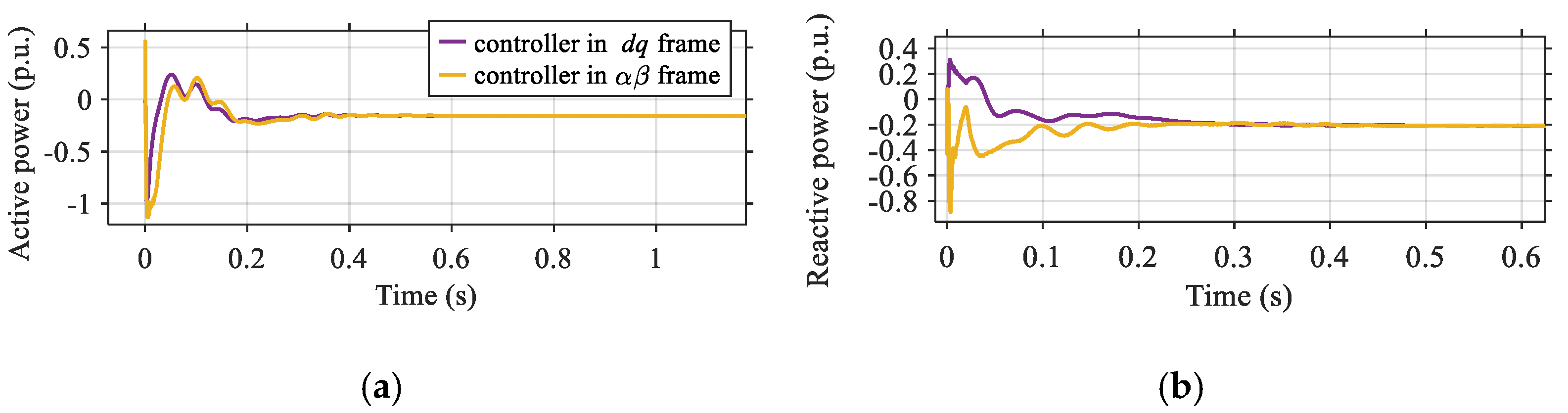The initial responses of the VSC using dq and $\alpha \beta$ reference frames are depicted in Figure 16.

According to this figure, at the commencement of the simulation, the VSC’s pivotal function in energizing the MT-HVDC grid through its droop control strategy manifests as a substantial negative active power output. This negative value indicates that the VSC is injecting power into the MT-HVDC grid. Once the DC voltage stabilizes, the active power output reduces to -0.2 p.u., signifying that excess generation from the DG sources, combined with a relatively weak AC grid, is fed into the MT-HVDC grid.

A comparative analysis of the VSC’s performance using the two referenced control strategies shown in Figure 16a reveals that both controllers exhibit approximately similar active power response characteristics. However, an examination of Figure 16b demonstrates that the reactive power in the $\alpha \beta$ reference frame experiences a peak deviation of 0.6 p.u. from its steady-state condition, which is recorded at −0.2 p.u. In comparison, the dq reference frame displays a maximum fluctuation of 0.5 p.u. from the same steady-state value of −0.2 p.u. Notably, both control strategies achieve the same settling time around 0.3 s.

7.2. Case Study 2: Operation Under Large Load Changes

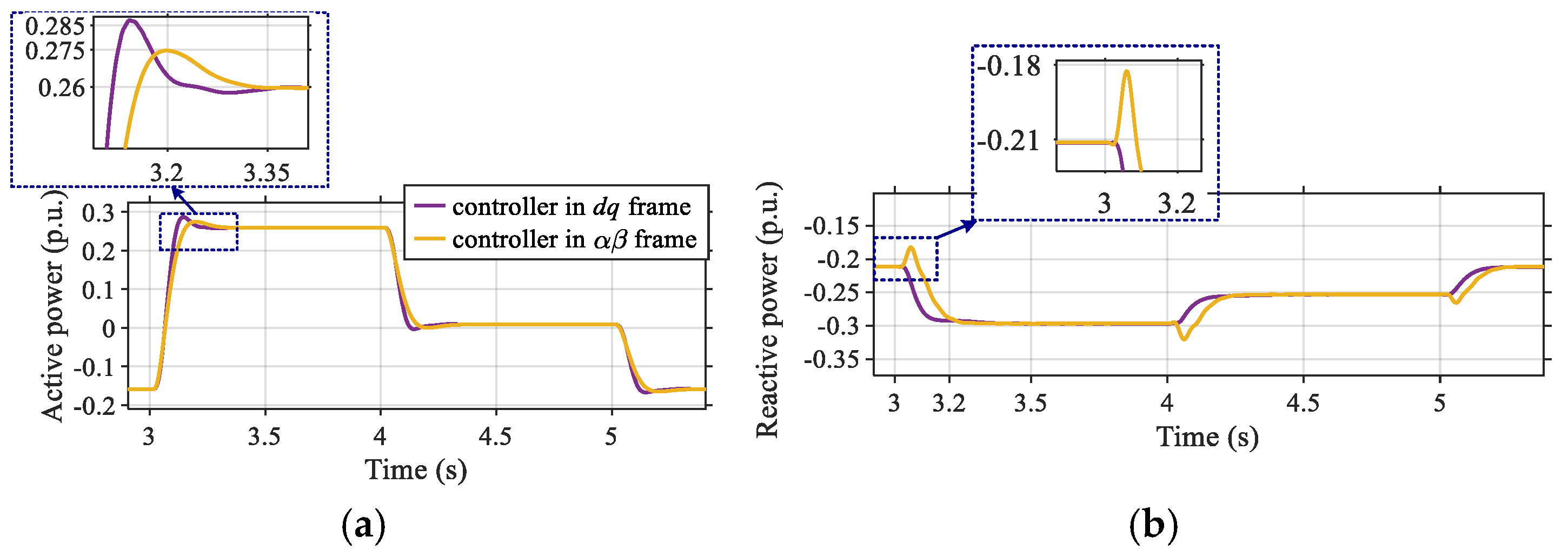
The following analysis presents the variation in the VSC’s active power output in response to a 500 MW load increase at the Ba-A1 feeding bus at t = 3 s. This is subsequently followed by a 300 MW load reduction at t = 4 s and an additional 200 MW reduction at t = 5 s. In Figure 17a, the dq frame controller exhibits a quicker dynamic response to fluctuations in active power, resulting in an overshoot of 9.6% in active power output. In contrast, the $\alpha \beta$ frame controller shows a minor overshoot of 5.8%. Figure 17b further demonstrates that the dq frame controller achieves a more favorable reactive power output, characterized by a reduced settling time of approximately 0.1 s. Meanwhile, the $\alpha \beta$ frame controller experiences a misdirection of 0.03 p.u. along with a longer settling time of 0.2 s. Both control strategies effectively decouple the active and reactive power loops; however, their inherent coupling arises from their interaction with the same load dynamics. Consequently, achieving precise active power regulation necessitates a corresponding variation in reactive power, which is particularly evident in the controller operating in the $\alpha \beta$ frame.

7.3. Case Study 3: Operation Under Three-Phase-to-Ground Fault

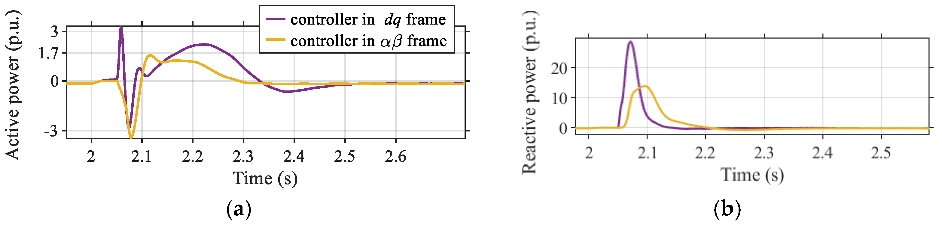
To further evaluate the controllers’ performance under adverse conditions, we assumed that at t = 2 s, a three-phase-to-ground temporary fault with a fault resistance of 0.1 Ω and a ground resistance of 0.8 Ω occurs at the Ba-A1 bus. It is important to note that this comparison is solely intended for analyzing the dynamics of the VSC under each control scheme, and does not account for any protection mechanisms.

In Figure 18a, analysis reveals that both controllers exhibit approximately similar deviations in active power. However, the $\alpha \beta$ frame controller provides a more rapid convergence to its reference values during the post-fault period, achieving this within 0.3 s. In contrast, the dq frame controller requires approximately 0.5 s for the same process. Conversely, Figure 18b illustrates that the dq controller shows a significantly higher reactive power response to faults, reaching 27 p.u., compared to the 15 p.u. observed for the $\alpha \beta$ frame controller. The data indicates that the $\alpha \beta$ frame controller is lagging in fault response. This behavior connects directly to the synchronization analysis of Section 5 and the FLL/PLL estimator expressions in Table 1: because the FLL locks onto frequency rather than phase, it responds more gradually to the abrupt fault transient than the phase-tracking PLL, consistent with the smaller overshoot and slower settling already shown for the FLL in Figure 14.

7.4. Case Study 4: Operation Under Unbalanced Grid Voltages

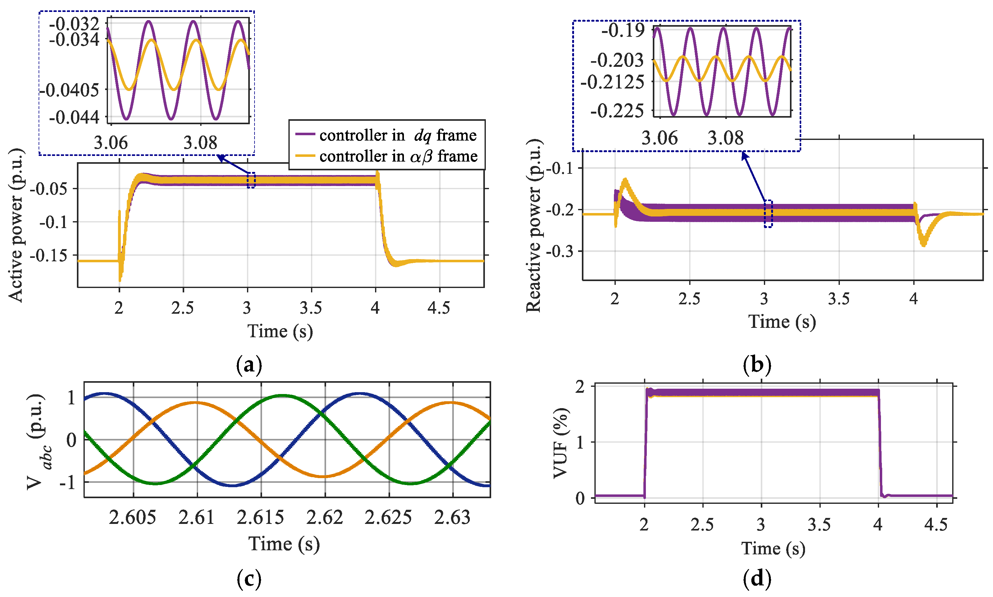
In the next analysis, to show the dq- and $\alpha \beta$-based controllers’ responses to unbalanced loads, the 500 MW single-phase load is applied to phase b. The voltage unbalance factor (VUF), which is the ratio of negative sequence voltage to positive sequence voltage [54], is used in this analysis to evaluate the ratio of imbalances in the grid. The data illustrated in Figure 19a highlight that $\alpha \beta$ reduces the fluctuations in active power output by 45.83% in comparison with the dq frame controllers when subjected to about 2% voltage imbalances. By comparing the fluctuations of reactive power in Figure 19b, it is revealed that the $\alpha \beta$ control method shows a 72.86% reduction in fluctuations compared to the dq reference controller. As previously discussed, managing the VSC in the $\alpha \beta$ frame circumvents the necessity for phase sequence separation, which is essential to employ a double SRF when using dq frame control, particularly in unbalanced scenarios.

It is important to note that the controller in the $\alpha \beta$ frame does experience such fluctuations. These variations stem from the distributed generation sources and the dynamics associated with the weak AC grid A0, which impact the converter’s output power. Nevertheless, the $\alpha \beta$ frame controller effectively reduces these fluctuations. This result follows from the PR controller’s infinite gain at both ±${\omega }_e$ established in Section 4 and Table 1: the single PR block inherently regulates the positive- and negative-sequence currents, that the dq frame can remove only by adding a double SRF (Section 2), which accounts for the markedly lower fluctuations observed here.

Also, the grid voltage depicted in Figure 19c is approximately equivalent for both controllers, with one being highlighted to illustrate its imbalance. This equivalence is clearly demonstrated in the VUF for both controllers, which are approximately equal and below 2% for both controllers.

7.5. Case Study 5: Operation in a Harmonic-Rich Grid

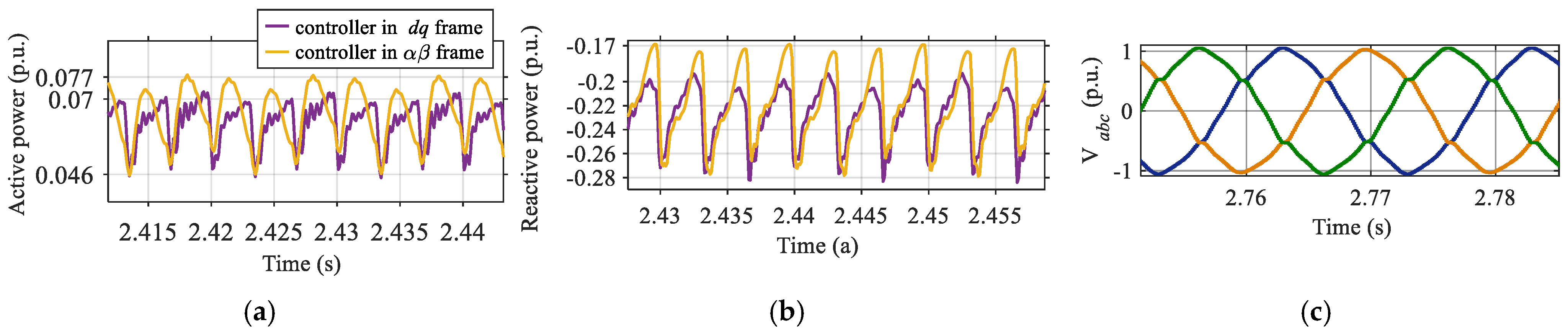
To evaluate the performance of these control techniques in the presence of harmonics within the grid, a 400 MW non-linear load is introduced to the Ba-A1 grid. The results for the two controllers are presented in Figure 20. The $\alpha \beta$ frame controller exhibits a fluctuation of 0.031 p.u. in active power and a variation of 0.11 p.u. in reactive power. In contrast, the dq frame controller demonstrates lower fluctuations, with values of 0.024 p.u. for active power and 0.08 p.u. for reactive power. However, it is noteworthy that the dq frame controller experiences higher frequency fluctuations. The grid voltage depicted in Figure 20c is almost equal for both controllers. The voltages in the first test (controller in dq frame) are selected to highlight the grid voltages along with their associated harmonics. 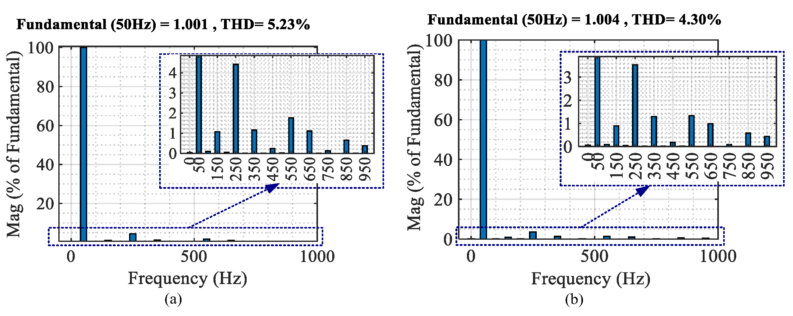But to be more precise, Figure 21 shows the one-cycle Fast Fourier Transform (FFT) analysis of phase a grid voltage, initiated at 2.5 s. The FFT is performed over a single fundamental period (a 20 ms window at 50 Hz) using the simulation sampling interval of 0.1 ms (a 10 kHz sampling rate), which provides a frequency resolution of 50 Hz and resolves harmonic components up to the Nyquist frequency of 5 kHz.

The FFT analysis indicates that the total harmonic distortion (THD) for the dq frame controller is 5.23%, while the $\alpha \beta$ controller demonstrates a THD of 4.3%. This results in a 17.7% improvement in harmonic mitigation efficiency with the implementation of the $\alpha \beta$ frame.

This difference is consistent with the harmonic-handling rows of Table 1, where the αβ frame employs resonant terms at $h {\omega }_e$ and the dq frame uses notch filtering at (h − 1) ${\omega }_e$. Since the dedicated harmonic compensators of both frames, the parallel resonant terms in the αβ frame and the cascaded notch filters in the dq frame, are disabled here to preserve a fair baseline, the modest THD advantage of the αβ frame is attributable to the inherent loop-gain characteristics of the baseline PR and PI regulators: the proportional-resonant structure presents a comparatively higher and better-shaped loop gain at the low-order harmonic frequencies than the dq-frame PI regulator, whose high gain is concentrated near DC and whose harmonic response is further affected by the Park transformation.

It is important to note that the incorporation of parallel resonant terms in the $\alpha \beta$ frame controller, as well as the use of cascaded notch filters in the dq frame controller, can effectively mitigate these THDs. However, to ensure a fair comparison between these two pure control strategies, these elements have been excluded from the current analysis.

8. Conclusions

This study highlighted the existing gaps in the literature regarding a comprehensive, standard-compliant comparison of control methodologies for VSCs connected to HVDC systems. It addressed several essential topics that have not been cohesively analyzed within a unified framework, including fundamental control principles, mathematical modeling, and filtering techniques. Furthermore, the study provided an in-depth examination and comparison of PLLs and FLLs, which are key synchronization components in both reference frames. The representations of the VSC in the $\alpha \beta$ and dq reference frames, along with corresponding tuning techniques based on the power converter’s average model, were also analyzed. Finally, simulation results obtained under standard operating conditions confirmed the theoretical discussions regarding the performance of the presented VSC control strategies. The main findings of this work are summarized as follows:

• The mathematical representations of the $\alpha \beta$ and dq reference frames show that, although the dq frame requires an additional Park transformation, it converts AC variables into DC quantities in steady state, thereby simplifying the decoupled control of active and reactive power in VSCs. This property makes the dq frame particularly advantageous for applications such as virtual synchronous machines (VSMs).
• The FLL demands precise tuning and more sophisticated filtering techniques, such as DSCs. In contrast, the PLL used for synchronization in the dq frame is characterized by its simpler architecture and utilizes easy filtering methods, like the MAF.
• The FLL shows enhanced robustness in weak AC grid environments that experience significant frequency fluctuations, whereas the PLL demonstrates more precise synchronization under low-frequency variations.
• Although the $\alpha \beta$ frame intrinsically decouples active and reactive power without needing additional decoupling techniques, which is critical in the dq frame, its implementation is more complex due to the requirement for advanced synchronization mechanisms and a reference signal generation block.
• The $\alpha \beta$ frame controller exhibits a delay relative to the dq frame under fault conditions, primarily due to its reliance on an FLL. The FLL inherently relies on frequency instead of phase angle.
• The VSC utilizing an $\alpha \beta$ frame controller demonstrates enhanced resilience against voltage imbalances and harmonic distortion.
• It should be noted that the present comparison is based on simulation studies within the standard Cigre-DCS 3 framework and therefore does not capture certain non-ideal hardware factors encountered in practical implementations, such as semiconductor switching non-linearities, dead-time effects, measurement noise, and the finite computational resources of the digital controller. Future work will focus on experimental and hardware-in-the-loop validation of the presented comparison in weak and converter-dominated AC grids.