A Bayesian Framework for Probabilistic Wind Turbine Technology Projections: Multi-Region Validation and Application to Climate-Aware Energy Yield Estimation

Abstract

Long-term energy system planning depends on projections of future wind turbine characteristics, yet existing approaches rely on either costly expert elicitation or deterministic trend extrapolation without formal uncertainty quantification. We present a Bayesian logistic framework that models the temporal evolution of hub height, rotor diameter, and specific power as physically constrained growth and decay processes, producing full posterior predictive distributions via Markov Chain Monte Carlo sampling. The framework is validated across three major onshore wind markets: Austria (534 turbines, 2000–2025), Germany (31,202 turbines, 1988–2026), and the United States (71,457 turbines, 1986–2025); spanning different market structures, regulatory environments, and data availability. Systematic benchmarking against linear, polynomial, and maximum-likelihood alternatives demonstrates superior hindcast performance, particularly for long-range projections where physical saturation constraints become relevant. Prior sensitivity analysis reveals that posteriors are robust for data-rich regions but honestly reflect prior influence for small datasets, identifying where expert knowledge is essential. We extend the framework to climate-aware energy yield estimation by propagating turbine posteriors through synthetic power curves and site-specific wind resource projections under SSP2-4.5 and SSP5-8.5, decomposing the total uncertainty into technology and climate components. When climate uncertainty is measured by scenario spread alone, technology uncertainty dominates. However, accounting for the full inter-model spread across 13 CMIP6 global climate models reveals that climate uncertainty becomes substantial (14–56%) and region-dependent, underscoring that both sources require explicit quantification. The open-source pipeline is designed for direct adoption in energy system planning workflows.

1. Introduction

Long-term energy system planning requires credible assumptions about future wind turbine characteristics (hub height, rotor diameter, and specific power). Yet existing approaches either rely on costly expert elicitation surveys that resist automated updating or on naive trend extrapolations that lack both physical saturation constraints and uncertainty quantification. We present a Bayesian logistic framework that bridges this gap: it combines physically motivated growth and decay models with configurable prior distributions, producing full posterior predictive distributions for turbine metrics and derived quantities such as rated capacity and annual energy production. The framework is validated across three major wind markets (Austria, Germany, and the United States); benchmarked against linear, polynomial, and maximum-likelihood alternatives; and extended to a climate-aware energy yield estimation by coupling turbine projections with site-specific wind resource scenarios under SSP2-4.5 and SSP5-8.5.

1.1. Expert Elicitation and Industry Projections

The most prominent approach to projecting future turbine characteristics is expert elicitation. Wiser et al. [1] surveyed more than 140 wind energy experts worldwide and projected LCOE reductions of 37–49% by mid-century. Beiter et al. [2], drawing on the same expert elicitation, reported median expectations for onshore turbines of 5.5 MW rated capacity with 130 m hub heights and 174 m rotor diameters by 2035. They extended this analysis to the “wind power plant of the future,” incorporating not only turbine scaling but also wake steering and hybrid plant concepts. Industry roadmaps from IEA Wind TCP Task 26 [3] define three technology scenarios for 2030 onshore wind: business-as-usual (325 W/m², 100 m hub height), likely (250 W/m², 125 m), and ambitious (175 W/m², 150 m). The NREL Annual Technology Baseline [4] projects specific power values ranging from 192 W/m² (technology class T3, targeting low-wind sites) to 275 W/m² (T2) for 2030 configurations. IRENA’s “Future of Wind” report [5] projected onshore capacities of 4–5 MW by 2025 with capacity factors reaching 30–55% by 2030 and up to 58% by 2050.

While these projections are invaluable, they share a fundamental limitation: they produce point estimates or scenario ranges rather than formal probability distributions, and they cannot be automatically updated as new installation data become available. Current grid development plans reveal a related methodological disconnect: while transmission system operators increasingly employ probabilistic adequacy assessments, e.g., ENTSO-E’s European Resource Adequacy Assessment (ERAA) uses 540 Monte Carlo simulation years [6], the underlying turbine technology assumptions remain deterministic. The German grid development plan (Netzentwicklungsplan, NEP 2037/2045) assumes a single reference turbine of 6.2 MW rated capacity, 165 m hub height, and 160 m rotor diameter (≈308 W/m²) [7], while Austria’s APG plans with approximately 2000 full-load hours implying ≈300 W/m² [8]. Our framework addresses this “probabilistic gap” by encoding expert knowledge as Bayesian priors that are systematically updated with observed data, yielding full posterior distributions that quantify both the most likely trajectory and its uncertainty.

1.2. Technology S-Curves and Logistic Diffusion Models

Technology adoption in energy systems typically follows sigmoidal trajectories. Zielonka et al. [9] compared 12 S-curve model variants, including Bass, Richards, and Gompertz formulations, across 2148 Swiss municipalities, demonstrating the superiority of probabilistic over deterministic approaches for capturing diffusion heterogeneity. Way et al. [10] applied probabilistic cost forecasting across more than 50 energy technologies, showing that empirically grounded projections outperform simulation-based approaches.

However, these studies model market diffusion(installed capacity, adoption rates, or costs) rather than physical turbine characteristics. A logistic growth curve for installed capacity tells energy planners how much wind power will be deployed but not what the turbines will look like and it is the latter that determines capacity factors, wake losses, and grid integration requirements. Our work applies logistic models to the turbine design parameters themselves, treating hub height and rotor diameter as quantities subject to physical saturation (regulatory height limits, transport constraints, aerodynamic scaling laws) and specific power as exhibiting logistic decay toward a market-driven lower bound.

1.3. Descriptive Turbine Trend Analysis

Several studies document historical trends in turbine dimensions. Bošnjaković et al. [11] reviewed 35 years of turbine component evolution, concluding that rotor diameters have more than doubled and rated capacities increased eightfold. The U.S. Wind Turbine Database (USWTDB; Hoen et al. [12]) and the German Marktstammdatenregister [13] provide comprehensive, publicly available installation records spanning decades. Most recently, the GOWIRES dataset [14] compiled 416,417 onshore turbines across 89 countries with site-specific historical and future wind resource data. IRENA reports that the average rotor diameter of newly commissioned turbines reached 206 m in 2023 (an 84% increase since 2010), with hub heights averaging 126 m [15]; these figures include both onshore and offshore installations.

These databases are essential for our work, but the existing analyses remain descriptive: they report observed trends without projecting them forward probabilistically. Our contribution is to turn these rich datasets into inputs for a Bayesian inference framework that extrapolates trends while respecting physical constraints and quantifying uncertainty.

1.4. Bayesian Methods for Small-Sample Technology Forecasting

Bayesian inference offers well-known advantages for small-sample settings: prior distributions regularize estimates, posterior distributions naturally quantify uncertainty, and the framework does not require the asymptotic assumptions underlying maximum-likelihood estimation [16]. These properties are particularly relevant for emerging wind markets or regions with limited installation histories, where frequentist approaches to logistic curve fitting may produce unstable or physically implausible parameter estimates. In the early exponential growth phase, before the inflection point or saturation is observed, the growth rate k and carrying capacity L are mathematically strongly correlated, and multiple parameter sets can produce nearly identical fits while implying vastly different saturation levels.

Our Austrian dataset (534 turbines, 2000–2025) exemplifies this challenge: only 25 years of data, concentrated in the exponential growth phase of the logistic curve, with no visible saturation onset. Furthermore, it is a limited set in terms of location (clustered in north-eastern Austria) and size compared to installed capacity in Austria. Bayesian priors informed by physical constraints and expert knowledge anchor the saturation level even when the data alone cannot identify it. We demonstrate through prior sensitivity analysis that the posteriors converge across informative, weakly informative, and diffuse prior specifications when sufficient data are available (US dataset) while honestly reflecting prior influence when data are limited (Austrian dataset).

1.5. Synthetic Power Curves and Future Turbine Designs in Energy System Models

Energy system models and wind resource assessments require power curves for turbines that do not yet exist. Ryberg et al. [17] addressed this by developing a synthetic power curve generator parameterized by specific power, enabling simulation of “advanced turbine designs” for European onshore wind potential assessments. Their key finding, that using contemporary instead of future turbine designs systematically underestimates wind energy potential, motivates the need for probabilistic turbine projections.

However, existing applications usedeterministic future turbine scenarios: a single hub height, a single rotor diameter, and a single specific power value per scenario. This discards the considerable uncertainty in technology evolution. Our framework closes this gap by producing distributions of turbine characteristics that can be propagated through the power curve generation and energy yield calculation chain, yielding probabilistic annual energy production estimates rather than point forecasts.

1.6. Climate Change Impacts on Wind Resources

Climate change introduces a second source of uncertainty into long-term energy planning. Pryor and Barthelmie [18] showed that internal climate variability currently dominates over forced trends for most major wind regions, though detectable changes emerge in high-emission scenarios. Martinez and Iglesias [19] projected significant declines in global wind power density by 2100, particularly in Northern Hemisphere mid-latitudes, with regional changes ranging from $-50$% to $+60$% depending on season and location. The GOWIRES dataset [14] provides site-specific Weibull parameters under SSP2-4.5 and SSP5-8.5 from 13 statistically downscaled CMIP6 global climate models.

Critically, these climate impact studies use fixed, contemporary turbine designs. The interaction between technology evolution and resource non-stationarity, how future turbines with lower specific power and higher hub heights will perform in changed wind climates, has not been quantified probabilistically. Our application showcase addresses exactly this coupling: we propagate both technology uncertainty (from our Bayesian posteriors) and climate uncertainty (from GOWIRES scenarios) through the energy yield chain, decomposing the total variance into its technology and climate components.

The framework is explicitly designed as a data-driven baseline projection tool rather than a model of turbine engineering innovation. It captures the trajectory that market data reveal, including saturation effects where observed technology trends have stabilized, and produces uncertainty bands that honestly reflect the limits of extrapolation from historical observations. Where domain experts anticipate technological breakthroughs (e.g., segmented blades enabling specific power below 200 W/m²), the configurable prior distributions provide a principled mechanism to incorporate such knowledge without conflating it with data-driven inference. Without expert modification, the framework delivers a conservative, market-consistent baseline, precisely the type of input that energy system modelers and grid planners require for robust scenario analysis.

1.7. Contribution and Paper Structure

In this paper, we propose a Bayesian logistic framework for probabilistic wind turbine technology projections and demonstrate its application to climate-aware energy yield estimation. Our specific contributions are:

• A modular Bayesian logistic growth/decay model with physically motivated, configurable priors for hub height, rotor diameter, and specific power;
• Multi-region validation across Austria (534 turbines), Germany (31,202 turbines), and the United States (71,457 turbines), spanning different market structures, regulatory environments, and data availability;
• Systematic benchmarking against linear, polynomial, and maximum-likelihood logistic alternatives, including hindcast validation and prior sensitivity analysis;
• An end-to-end application that propagates turbine uncertainty through synthetic power curves and climate-adjusted wind profiles to yield probabilistic annual energy production estimates in SSP2-4.5 and SSP5-8.5 scenarios;
• An open-source code and reproducible analysis pipeline to facilitate adoption by the energy planning community.

The remainder of this paper is organized as follows: Section 2 describes the datasets and study regions. Section 3 presents the Bayesian methodology, benchmark models, and energy yield framework. Section 4 reports the results across all three regions, including projections, benchmarks, sensitivity analysis, and the climate-aware application. Section 5 discusses implications, limitations, and future work. Section 6 concludes.

2. Data and Study Regions

This study draws on three partially publicly available wind turbine installation datasets spanning different market sizes, regulatory environments, and temporal coverage.

Table 1. Summary of regional wind turbine datasets after quality control. For Austria, interquartile ranges are reported instead of full ranges to preserve data confidentiality.

Region	Source	Period	N (raw)	N (QC)	Med. HH2024	Med. RD2024	Med. SP2024
					[m] (IQR)	[m] (IQR)	[W/m2](IQR)
AT	IGW/UVP	2000–2025	605	534	168 (151–169)	162 (149–163)	323 (310–349)
DE	MaStR	1988–2026	42,429	31,202	160 (124–165)	149 (138–160)	291 (277–327)
US	USWTDB	1986–2025	75,727	71,457	105 (98–117)	140 (127–150)	223 (221–238)

summarizes the key characteristics after quality control.

2.1. Austria (AT)

The Austrian dataset was compiled from two sources: the Interessengemeinschaft Windkraft (IGW) project database and Environmental Impact Assessment (Umweltverträg-lichkeitsprüfung, UVP) filings. It contains 534 turbine entries spanning 2000–2025 after quality control. Austria’s wind fleet is concentrated in the eastern lowlands (Weinviertel, Marchfeld, Parndorfer Platte, Burgenland), with a rapid shift toward larger turbines after 2015 and ongoing installations in high Alpine locations. The dataset is small relative to the other two regions, representing a typical situation for smaller European markets where installation records may be incomplete or fragmented. The 534 entries represent approximately 38% of Austria’s estimated commissioned fleet of ≈1400 turbines, with higher coverage for recent installations where technical specifications are more systematically recorded in IGW and UVP filings. The under-represented entries are predominantly older, smaller machines for which technical specifications were archived less systematically; coverage for the most recent commissioning years is close to complete. This selection may introduce a modest bias toward more recent, well-documented turbines, which we discuss in Section 5.7. Austria’s national grid development plan (APG NEP 2025) targets 16.5 GW of installed wind capacity by 2040, assuming approximately 2000 full-load hours per turbine, consistent with a specific power of ≈300 W/m² at typical Austrian sites [8].

2.2. Germany (DE)

German turbine data were obtained from the Marktstammdatenregister (MaStR), the official registry of energy generation units maintained by the Bundesnetzagentur [13]. After filtering for onshore wind turbines with valid commissioning dates, hub heights, rotor diameters, and rated capacities, the dataset comprises 31,202 turbines spanning 1988–2026. The 2026 entries are units already in operation as recorded in the MaStR at the extraction date, not merely planned or commissioned-but-not-yet-built projects; excluding them changes the German posterior medians by less than 0.1%. Germany represents the largest European onshore wind market, with a well-documented evolution from early sub-megawatt machines to modern 5+ MW platforms. The dataset captures the full S-curve trajectory, including an early growth phase in the 1990s and incipient saturation in hub height after 2015. The German grid development plan (NEP 2037/2045) assumes a deterministic reference turbine of approximately 6 MW rated capacity with hub heights of ≈165 m and specific power of ≈300 W/m², with 2600 full-load hours projected for 2037 [7].

2.3. United States (US)

The United States Wind Turbine Database (USWTDB, Version 8.3, March 2026; Hoen et al. [12]) provides the most comprehensive national turbine inventory available. After restricting to continental US onshore turbines with complete technical specifications, the dataset contains 71,457 turbines spanning 1986–2025. The US dataset offers the longest temporal coverage, including a clearly visible lag phase in the 1980s–1990s when turbine dimensions evolved slowly, followed by rapid growth in the 2000s. Notably, US hub heights are systematically lower than those of their European counterparts (≈105 m median in 2024 vs. ≈160 m in Germany), reflecting different regulatory frameworks, land availability, and wind resource characteristics. The US market exhibits the most aggressive specific power decline globally, driven by the Production Tax Credit (PTC) structure that incentivizes maximizing energy production per unit of rated capacity [20].

2.4. Quality Control

A uniform quality control procedure was applied to all three datasets:

• Completeness Only entries with valid values for commissioning year, hub height, rotor diameter, and rated capacity were retained.
• Physical plausibility: Entries were excluded if hub height $<20$ m or >250 m, rotor diameter $<10$ m or >250 m, specific power $<100$ W/m² or >800 W/m², or rated capacity $<100$ kW.
• Geographic filtering: For the US, offshore turbines and installations outside the continental states were removed. For Germany, offshore entries were excluded via the MaStR location classification.
• Duplicate removal: Entries with identical location, year, and technical specifications were deduplicated.

Specific power was computed as $\mathrm{SP}=P_{\mathrm{rated}}/A_{\mathrm{rotor}}$, where $A_{\mathrm{rotor}}=\pi {(D/2)}^2$ is the rotor swept area.

Table 2. Number of entries excluded at each quality control stage.

Region	3. Geogr.	1. Incomplete	2. Implausible	4. Duplicates	Final N	Total Excl.
AT	—	69	0	2	534	71
DE	1849	8289	1089	0	31,202	11,227
US	415	3642	213	0	71,457	4270

reports the number of entries excluded at each quality control stage.

2.5. Descriptive Overview

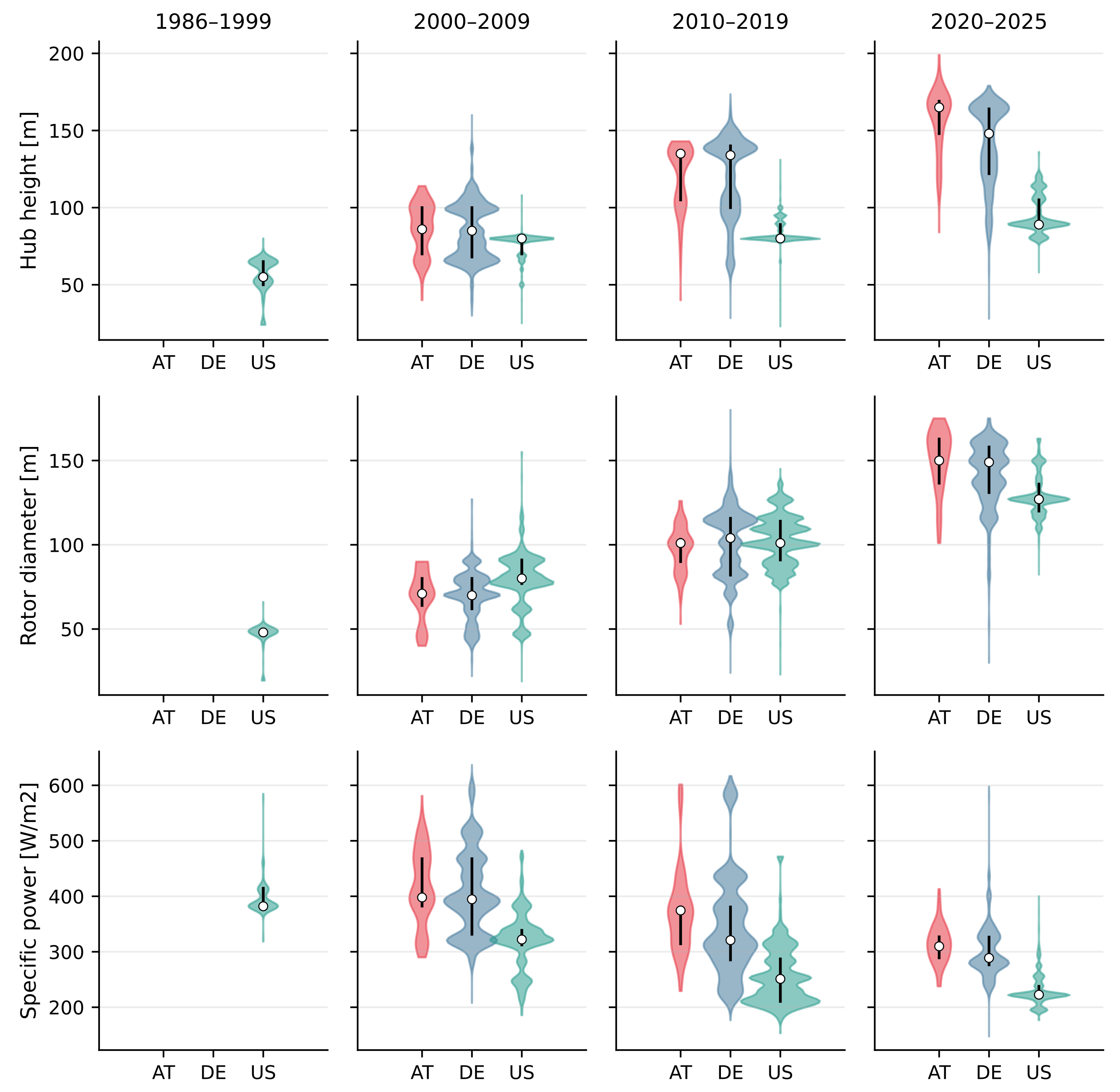
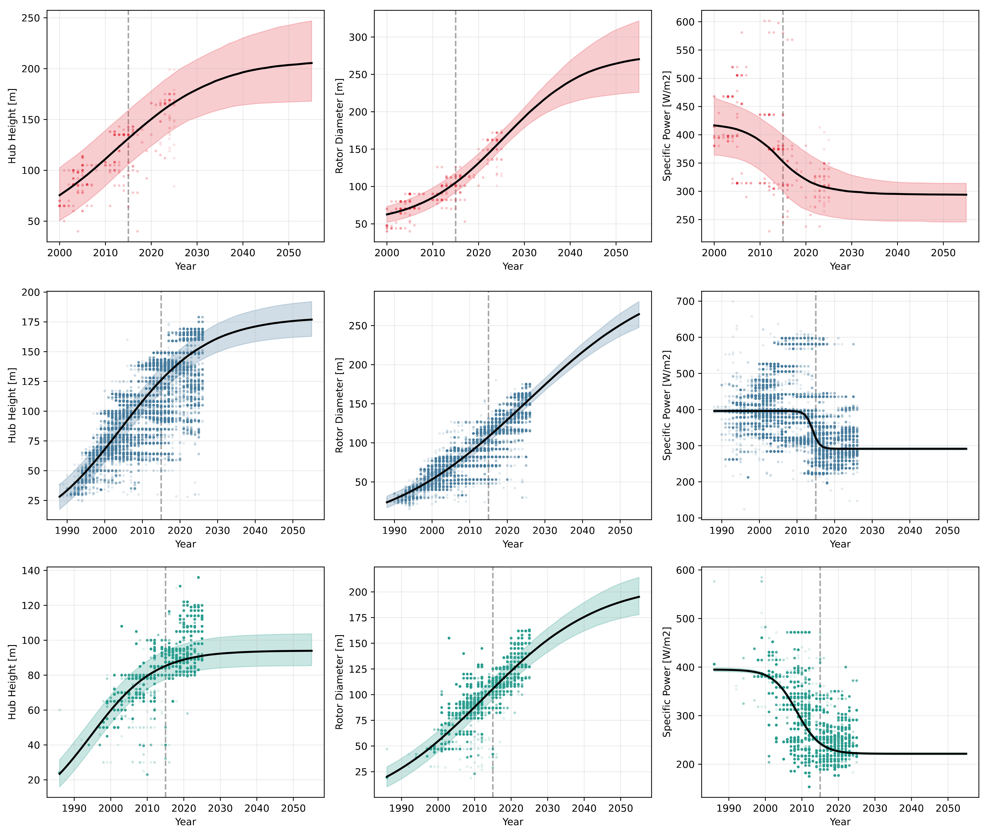
Figure 1 presents the distributional evolution of all three metrics across decades and regions. Hub heights and rotor diameters show a consistent upward shift across all markets, with Austria and Germany converging at the upper end (>150 m hub height, >140 m rotor diameter) by 2020–2025, while the US remains systematically lower (≈100 m hub height). Specific power exhibits a clear declining trend, most pronounced in the US (median ≈220 W/m² by 2020–2025) and more moderate in Europe (≈290–320 W/m²).

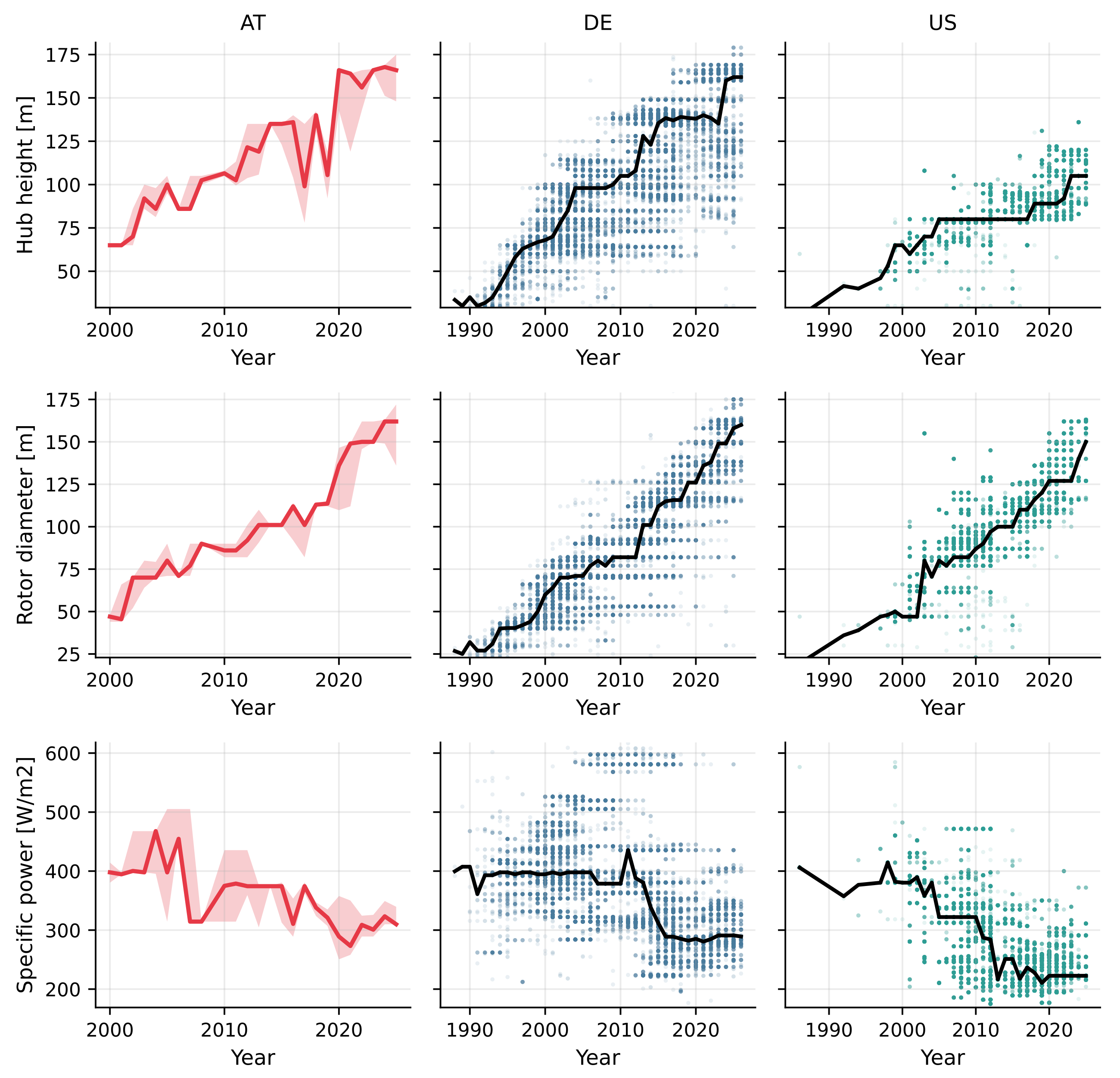
Figure 2 shows the annual time series for each region–metric combination. For Austria, where individual turbine data are subject to publication restrictions, we display annual medians with interquartile range bands rather than individual observations. For Germany and the US, individual turbine observations are shown alongside annual medians. The contrast in data density—534 Austrian entries versus 71,457 in the US—visually motivates the need for informative Bayesian priors in data-sparse settings.

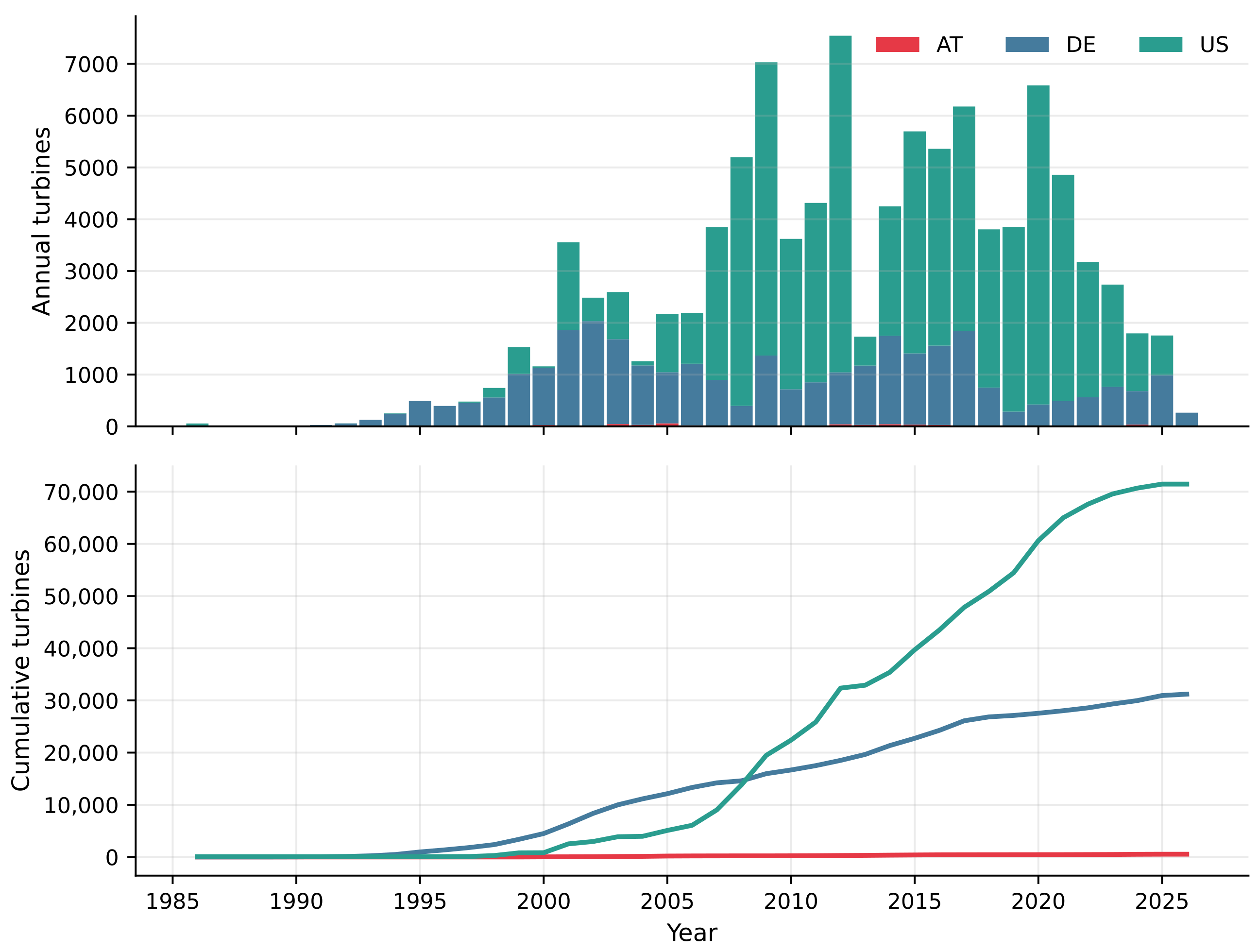
Figure 3 illustrates the annual installation volumes and cumulative fleet sizes across regions. The US dominates in total numbers, with peak installation years exceeding 7000 turbines (2012), while Austria’s annual installations rarely exceed 30 units. This two-orders-of-magnitude difference in sample size is a key challenge that our Bayesian framework is designed to address.

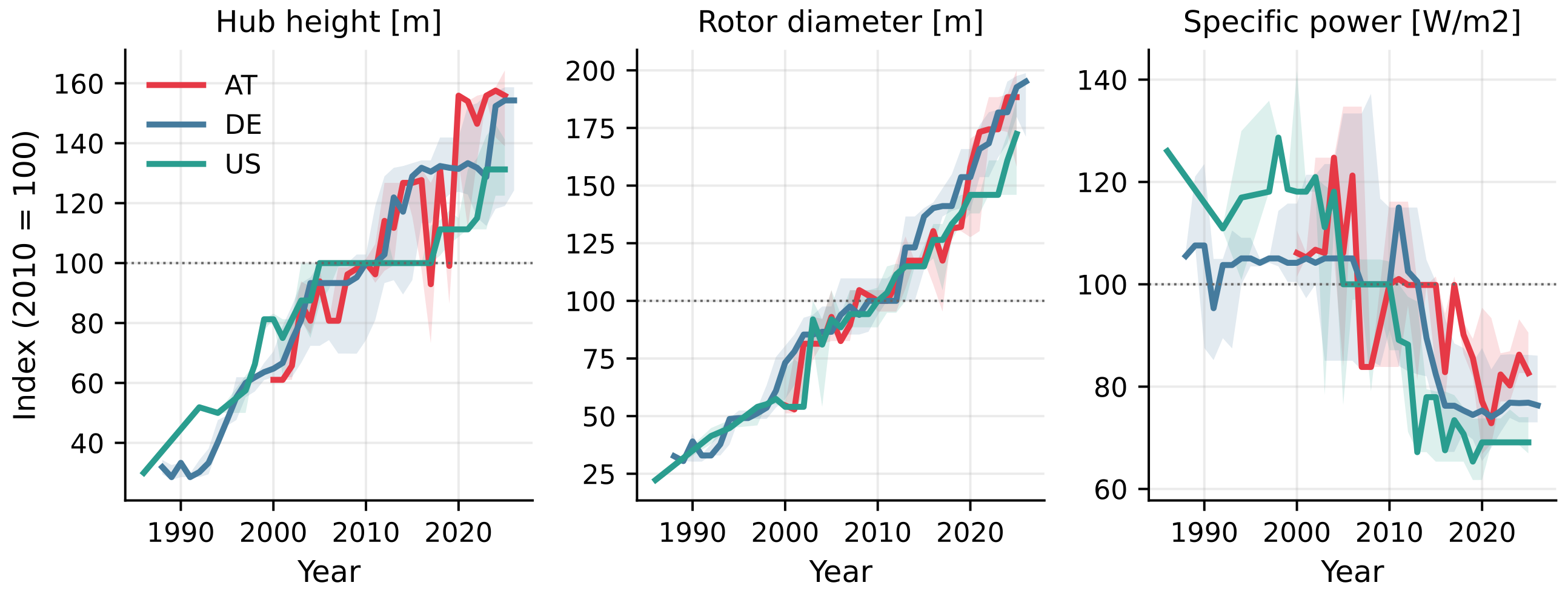
Figure 4 presents normalized index curves (2010 = 100) that enable direct comparison of relative growth rates across regions despite the vastly different absolute scales. Hub heights grew fastest in Austria (index ≈155 by 2024) and Germany (≈140), while US hub heights grew more slowly (≈130). For specific power, the US shows the steepest relative decline (index ≈ 70), consistent with its more aggressive adoption of low-specific-power turbines driven by the Production Tax Credit structure.

2.6. Climate Data

For the energy yield application (Section 3.6), site-specific wind resource parameters were obtained from the GOWIRES dataset [14], which provides historical (1989–2018) and future (2030–2059) Weibull scale and shape parameters for 416,417 global turbine sites in SSP2-4.5 and SSP5-8.5 scenarios derived from 13 statistically downscaled CMIP6 global climate models. We extracted Weibull parameters for representative reference sites in each study region: Weinviertel, Austria (47.5° N, 16.5° E); Schleswig-Holstein, Germany (53.5° N, 9.0° E); and the Nebraska Great Plains, USA (41.5° N, 99.5° W). All nine region–scenario combinations used GOWIRES-derived Weibull parameters based on the 50 nearest-neighbor turbines within the corresponding country (

Table 3. GOWIRES data provenance for reference sites. All parameters derived from spatial averaging over 50 nearest-neighbor turbines.

Region	Reference Site	N Neighbors	Max. Dist. [km]	Hist. PLE ($\mathit{\alpha }$)
AT	Weinviertel (47.5° N, 16.5° E)	50	45.2	0.227
DE	Schleswig-Holstein (53.5° N, 9.0° E)	50	6.1	0.233
US	Nebraska (41.5° N, 99.5° W)	50	7.9	0.186

). No literature fallback values were required. GOWIRES provides Weibull parameters individually for each of the 13 CMIP6 global climate models, enabling a full inter-model variance decomposition in addition to the inter-scenario comparison (Uncertainty Decomposition Section).

3. Methodology

3.1. Bayesian Logistic Growth and Decay Models

We model the temporal evolution of each turbine metric using logistic functions that incorporate physical saturation constraints.

3.1.1. Logistic Growth (Hub Height, Rotor Diameter)

Hub height and rotor diameter are modeled as logistic growth processes:

$$y\left(t\right)=y_0+{\displaystyle \frac{L}{1+exp\left(-k(t-t_0)\right)}},$$

(1)

where $y_0$ is the baseline value before significant growth, L is the carrying capacity (the maximum additional increase from $y_0$), $k>0$ is the growth rate, and $t_0$ is the inflection point (year of maximum growth rate). The asymptotic upper limit is $y_0+L$.

The logistic saturation of rotor dimensions is physically grounded in the square-cube law: doubling blade length increases swept area fourfold but blade mass eightfold, imposing diminishing returns on further scaling [11]. Additional constraints include road transport limits on tower base diameters (≈4.5 m) and tip-height restrictions in many jurisdictions. For hub heights, aviation regulations and structural engineering limits provide natural upper bounds that vary by region.

3.1.2. Logistic Decay (Specific Power)

Specific power exhibits a declining trend as rotors grow faster than rated capacity [20]. This is modeled as logistic decay:

$$y\left(t\right)=y_{min}+{\displaystyle \frac{L}{1+exp\left(k(t-t_0)\right)}},$$

(2)

where $y_{min}$ is the lower asymptotic bound, L is the total range of decline, $k>0$ governs the decay rate, and $t_0$ is the inflection point. The lower bound $y_{min}$ reflects engineering constraints: the NREL Big Adaptive Rotor (BAR) project targets 150 W/m² as a practical floor for 5 MW-class turbines, while DTU’s LowWind project has explored designs down to 100 W/m² for a 3.4 MW platform with a 208 m rotor [4].

3.1.3. Likelihood and Priors

The likelihood is specified as a Student-t distribution to provide robustness against outliers such as experimental or prototype turbines [21]:

$$y_i\sim \mathrm{StudentT}\left(\nu ,\mu \left(t_i\right),\sigma \right),$$

(3)

where $\mu \left(t_i\right)$ is the logistic function evaluated at the commissioning year of turbine i, $\sigma$ is the scale parameter, and $\nu$ is the degrees-of-freedom parameter, modeled as $\nu ={\nu }_{\mathrm{offset}}+2$ with ${\nu }_{\mathrm{offset}}\sim \mathrm{Exponential}(1/30)$ to ensure $\nu >2$ (finite variance) while allowing heavy tails. The Student-t likelihood automatically downweights extreme residuals, preventing individual outliers from distorting the inferred trend, a property that is particularly important given the heterogeneity of turbine installations within any single market. A comparison run with Gaussian likelihood for the German hub height model yielded posterior medians within 0.3% of the Student-t results, confirming that the likelihood choice affects tail behavior but not central projections. The Student-t is retained for its robustness to prototype and experimental turbine entries.

Prior distributions for all model parameters are specified as normal distributions with region-specific hyperparameters informed by physical constraints and domain knowledge. Table 4 reports the prior specifications for all region–metric combinations. The key physical motivations are:

• Hub height carrying capacity L: Bounded by regulatory height limits, aviation constraints, and structural engineering limits. The Austrian prior $\mathcal{N}(200,40)$ implies a median asymptotic hub height of $y_0+L\approx 260$ m; the Austrian Luftfahrtgesetz requires notification above 100 m AGL but imposes no hard height ceiling, while provincial building codes (planning regulations, different in Lower Austria and Burgenland) permit structures up to 200 m without individual aviation safety assessments. Turbines with tip heights exceeding 250 m are currently in the Austrian permitting pipeline. The German prior $\mathcal{N}(180,30)$ reflects the more constrained tip-height practice under the BImSchG, while the US prior $\mathcal{N}(120,30)$ reflects the FAA notification threshold of 152 m (500 ft) AGL, which functions as a de facto soft ceiling for most US installations [1].
• Rotor diameter carrying capacity L: Constrained by blade transport logistics, tower-top mass limits, and aerodynamic scaling laws (square-cube law).
• Specific power lower bound $y_{min}$: Set by the trade-off between energy capture and structural loads; values below ∼150 W/m² would require impractically large rotors for a given capacity.
• Growth rate k: Half-normal prior ($k>0$) reflecting monotonic growth/decay assumptions.

Table 4. Prior distributions for all region–metric combinations. $\mathcal{N}(\mu ,\sigma )$: Normal; $\mathcal{HN}\left(\sigma \right)$: Half-Normal (positive support); $\mathrm{Exp}\left(\lambda \right)$: Exponential. Physical motivations are discussed in the text.

Parameter	Physical Role	AT	DE	US
Hub Height (Logistic Growth)
L	Carrying capacity [m]	$\mathcal{N}(200,40)$	$\mathcal{N}(180,30)$	$\mathcal{N}(120,30)$
k	Growth rate [1/yr]	$\mathcal{HN}\left(0.3\right)$	$\mathcal{HN}\left(0.3\right)$	$\mathcal{HN}\left(0.3\right)$
$t_0$	Inflection year	$\mathcal{N}(2015,5)$	$\mathcal{N}(2008,5)$	$\mathcal{N}(2010,8)$
$y_0$	Baseline [m]	$\mathcal{N}(60,15)$	$\mathcal{N}(30,10)$	$\mathcal{N}(25,10)$
$\sigma$	Scale	$\mathcal{HN}\left(30\right)$	$\mathcal{HN}\left(30\right)$	$\mathcal{HN}\left(30\right)$
Rotor Diameter (Logistic Growth)
L	Carrying capacity [m]	$\mathcal{N}(200,50)$	$\mathcal{N}(180,40)$	$\mathcal{N}(170,40)$
k	Growth rate [1/yr]	$\mathcal{HN}\left(0.3\right)$	$\mathcal{HN}\left(0.3\right)$	$\mathcal{HN}\left(0.3\right)$
$t_0$	Inflection year	$\mathcal{N}(2015,5)$	$\mathcal{N}(2008,5)$	$\mathcal{N}(2008,8)$
$y_0$	Baseline [m]	$\mathcal{N}(40,15)$	$\mathcal{N}(20,10)$	$\mathcal{N}(15,10)$
$\sigma$	Scale	$\mathcal{HN}\left(30\right)$	$\mathcal{HN}\left(30\right)$	$\mathcal{HN}\left(30\right)$
Specific Power (Logistic Decay)
L	Decline range [W/m2]	$\mathcal{N}(150,40)$	$\mathcal{N}(150,30)$	$\mathcal{N}(200,40)$
k	Decay rate [1/yr]	$\mathcal{HN}\left(0.3\right)$	$\mathcal{HN}\left(0.3\right)$	$\mathcal{HN}\left(0.3\right)$
$t_0$	Inflection year	$\mathcal{N}(2012,5)$	$\mathcal{N}(2012,5)$	$\mathcal{N}(2005,5)$
$y_{min}$	Lower bound [W/m2]	$\mathcal{N}(250,30)$	$\mathcal{N}(250,30)$	$\mathcal{N}(200,30)$
$\sigma$	Scale	$\mathcal{HN}\left(50\right)$	$\mathcal{HN}\left(50\right)$	$\mathcal{HN}\left(50\right)$
Shared (all models)
$\nu$	Degrees of freedom	$\nu ={\nu }_{\mathrm{off}}+2$, ${\nu }_{\mathrm{off}}\sim \mathrm{Exp}(1/30)$

Table 4. Prior distributions for all region–metric combinations. $\mathcal{N}(\mu ,\sigma )$: Normal; $\mathcal{HN}\left(\sigma \right)$: Half-Normal (positive support); $\mathrm{Exp}\left(\lambda \right)$: Exponential. Physical motivations are discussed in the text.

Parameter	Physical Role	AT	DE	US
Hub Height (Logistic Growth)
L	Carrying capacity [m]	$\mathcal{N}(200,40)$	$\mathcal{N}(180,30)$	$\mathcal{N}(120,30)$
k	Growth rate [1/yr]	$\mathcal{HN}\left(0.3\right)$	$\mathcal{HN}\left(0.3\right)$	$\mathcal{HN}\left(0.3\right)$
$t_0$	Inflection year	$\mathcal{N}(2015,5)$	$\mathcal{N}(2008,5)$	$\mathcal{N}(2010,8)$
$y_0$	Baseline [m]	$\mathcal{N}(60,15)$	$\mathcal{N}(30,10)$	$\mathcal{N}(25,10)$
$\sigma$	Scale	$\mathcal{HN}\left(30\right)$	$\mathcal{HN}\left(30\right)$	$\mathcal{HN}\left(30\right)$
Rotor Diameter (Logistic Growth)
L	Carrying capacity [m]	$\mathcal{N}(200,50)$	$\mathcal{N}(180,40)$	$\mathcal{N}(170,40)$
k	Growth rate [1/yr]	$\mathcal{HN}\left(0.3\right)$	$\mathcal{HN}\left(0.3\right)$	$\mathcal{HN}\left(0.3\right)$
$t_0$	Inflection year	$\mathcal{N}(2015,5)$	$\mathcal{N}(2008,5)$	$\mathcal{N}(2008,8)$
$y_0$	Baseline [m]	$\mathcal{N}(40,15)$	$\mathcal{N}(20,10)$	$\mathcal{N}(15,10)$
$\sigma$	Scale	$\mathcal{HN}\left(30\right)$	$\mathcal{HN}\left(30\right)$	$\mathcal{HN}\left(30\right)$
Specific Power (Logistic Decay)
L	Decline range [W/m2]	$\mathcal{N}(150,40)$	$\mathcal{N}(150,30)$	$\mathcal{N}(200,40)$
k	Decay rate [1/yr]	$\mathcal{HN}\left(0.3\right)$	$\mathcal{HN}\left(0.3\right)$	$\mathcal{HN}\left(0.3\right)$
$t_0$	Inflection year	$\mathcal{N}(2012,5)$	$\mathcal{N}(2012,5)$	$\mathcal{N}(2005,5)$
$y_{min}$	Lower bound [W/m2]	$\mathcal{N}(250,30)$	$\mathcal{N}(250,30)$	$\mathcal{N}(200,30)$
$\sigma$	Scale	$\mathcal{HN}\left(50\right)$	$\mathcal{HN}\left(50\right)$	$\mathcal{HN}\left(50\right)$
Shared (all models)
$\nu$	Degrees of freedom	$\nu ={\nu }_{\mathrm{off}}+2$, ${\nu }_{\mathrm{off}}\sim \mathrm{Exp}(1/30)$

All parameter priors are specified independently; cross-parameter dependencies are learned from the data through the likelihood.

To confirm that these priors imply physically plausible behavior before any data are seen, we performed prior predictive checks for all nine region–metric combinations (500 prior draws each, evaluated for 1985–2060). Between 484 and 500 of the 500 drawn trajectories fall within a broad physical screening range (0–500 in the respective unit) in every combination, confirming that the priors concentrate on meaningful turbine-technology regimes rather than on implausible values. As shown in Appendix E (Figure A2), the prior trajectory envelopes are deliberately wide, while the posterior bands are markedly narrower for the data-rich regions (Germany and United States), visually demonstrating learning from the observations. Austria retains a comparatively broad posterior, an honest reflection of its short and sparse record rather than a modeling artifact.

3.2. Inference

All models were fitted using Markov Chain Monte Carlo (MCMC) sampling via the No-U-Turn Sampler (NUTS; Hoffman and Gelman [22]) implemented in PyMC v5 [23]. We used 10 chains with 4000 draws each after 1000 tuning iterations, a target acceptance probability of 0.95, and a fixed random seed for reproducibility. The elevated target acceptance rate (compared to the default of 0.80) was chosen to reduce the risk of divergent transitions in the tightly curved posterior geometry of logistic models, following recommendations in the PyMC documentation [23]. Convergence was assessed via the split-$\widehat{R}$ statistic (<1.05 for all parameters), effective sample size (ESS $>400$), and the absence of divergent transitions.

The Austrian dataset (N = 534) was used in its entirety. For computational efficiency, the German (N = 31,202) and US (N = 71,457) datasets were each subsampled to 5000 observations using stratified random sampling by year prior to fitting, preserving the temporal distribution of the data while reducing computation time. A sensitivity comparison between full-sample and subsampled fits for a subset of configurations confirmed negligible differences in posterior distributions (see Appendix A). For trend estimation on annual-resolution data, the effective information content is determined by the number of distinct years and the within-year variance, both of which are fully captured at N = 5000 (Appendix A). Beyond this threshold, additional observations sharpen the likelihood without improving posterior estimates while degrading MCMC geometry.

3.3. Derived Capacity and Uncertainty Propagation

Turbine rated capacity is a derived quantity:

$$P_{\mathrm{rated}}=\mathrm{SP}·{\displaystyle \frac{\pi D^2}{4}}·{10}^{-6}\left[\mathrm{MW}\right],$$

(4)

where $\mathrm{SP}$ is specific power [W/m²] and D is rotor diameter [m].

To propagate uncertainty, we draw from the posterior samples of both specific power and rotor diameter using matching sample indices, preserving the implicit correlation structure induced by shared temporal trends. This yields a full posterior distribution for rated capacity at each target year without requiring an explicit multivariate model across metrics. We note that this approach captures correlations arising from the shared time axis but does not model cross-metric dependencies within the Bayesian framework; extending to a joint multivariate model represents a natural direction for future work. We verified empirically that the shared-time-axis coupling captures the dominant dependence: independently shuffling the rotor-diameter and specific-power posterior samples changes the German AEP variance by only ≈1.5% (Uncertainty Decomposition Section), indicating that residual cross-metric structure beyond the common temporal trend is small for the present application.

3.4. Benchmark Models

To quantify the added value of the Bayesian logistic approach, we compare it against three simpler alternatives applied to the same data:

• Linear model: $y\left(t\right)=a+bt$, fitted by ordinary least squares.
• Quadratic polynomial: $y\left(t\right)=a+bt+c{t}^2$, fitted by ordinary least squares.
• MLE logistic: The same logistic functional form (Equations (1) or (2)), fitted by maximum-likelihood estimation via scipy.optimize.curve_fit without prior regularization.

All models are evaluated via hindcast validation: parameters are estimated using only data up to and including 2015, and predictions are compared against observations from 2016 to 2025. We report root mean squared error (RMSE), mean absolute error (MAE), and, for the Bayesian model, the continuous ranked probability score (CRPS) and empirical coverage of the 95% credible interval. A second hindcast split at 2018 is reported in the Appendix A, Appendix B, Appendix C, Appendix D and Appendix E as a sensitivity check. For the hindcast benchmark the Bayesian priors are identical to those used for the full-period fits. They encode physical and regulatory constraints (blade-transport limits, tip-height and aviation ceilings, the ≈150 W/m² engineering floor) that were established and documented well before the 2015 cutoff, so reusing them for the pre-2015 training set introduces no look-ahead information. CRPS was computed using the properscoringPython 3.12 library. The trapezoidal integration for the capacity factor (Equation (6)) uses 0.5 m/s resolution in production; a convergence test at 0.1 m/s confirmed negligible differences (<0.1% in AEP).

3.5. Prior Sensitivity Analysis

To assess the influence of prior specifications on posterior inferences, we repeated the Bayesian fits for three prior configurations:

• Informative (Set A): The primary prior specification described above, informed by physical constraints and domain knowledge.
• Weakly informative (Set B): Standard deviations of all normal priors doubled relative to Set A.
• Diffuse (Set C): Standard deviations quadrupled; saturation bounds replaced by wide uniform distributions.

We quantified prior sensitivity as the maximum relative deviation in posterior medians for the 2055 projection across all pairwise comparisons of the three prior sets (i.e., the single worst-case deviation across Sets A–B, A–C, and B–C), separately for each region and metric. The 2030 projections were also assessed; deviations are uniformly 40–60% smaller than the 2055 values, confirming that prior sensitivity increases with projection horizon. We expect the US dataset (long time series and large sample) to exhibit robust posteriors across all prior sets and the Austrian dataset (short time series and small sample) to show greater prior sensitivity. This contrast is itself a key result, demonstrating where informative priors are essential and where the data dominate.

3.6. Climate-Aware Energy Yield Estimation

To demonstrate the practical utility of the framework for energy system planning, we propagate the posterior distributions of turbine characteristics through the complete wind-to-power conversion chain.

3.6.1. Synthetic Power Curves

For each posterior sample i at a given target year, a synthetic power curve $P_i\left(v\right)$ is generated following the approach of Ryberg et al. [17]. The power curve is parameterized by specific power and rated capacity, with cut-in speed derived as a function of specific power ($v_{cut-in}\approx 3$–4 m/s), rated speed determined by the cubic relationship between wind speed and power, and cut-out speed fixed at 25 m/s. A cubic smoothstep transition is applied between cut-in and rated wind speed. This internal implementation follows the methodology of the RESKit toolkit (FZJ-IEK3) without requiring external dependencies.

3.6.2. Wind Profile Scaling

The reference Weibull distribution at 100 m is extrapolated to the posterior hub height $h_i$ using the power law:

$$A\left(h_i\right)=A_{100}{\left({\displaystyle \frac{h_i}{100}}\right)}^{\alpha },$$

(5)

where A is the Weibull scale parameter. Rather than adopting the generic $1/7$ value ($\alpha =0.143$), we use region-representative shear exponents derived from the GOWIRES reference neighbors of each study region (AT $\alpha =0.227$, DE $\alpha =0.233$, US $\alpha =0.186$; Table 3) as the main specification throughout. These are single representative exponents per study region—a substantial improvement over a universal value but not turbine-site-specific; operational single-site assessment would require locally measured or modeled shear profiles (Section 5.7). These values lie within the observed range of approximately 0.10 (convective conditions) to 0.25 (stable stratification). The fixed $\alpha =0.143$ case is retained only as a sensitivity comparison (Section 5.7). The Weibull shape parameter $\kappa$ is assumed height-invariant, consistent with standard practice in wind resource assessment [24], though this assumption becomes less accurate above ≈100 m where the transition from the surface layer to the Ekman layer alters the wind profile structure [24].

3.6.3. Capacity Factor and Annual Energy Production

The capacity factor for posterior sample i in climate simulation s is

$${\mathrm{CF}}_{i,s}={\displaystyle \frac{1}{P_{\mathrm{rated},i}}}{\int }_0^{v_{cut-out}}{P}_i\left(v\right)f_W(v;{\kappa }_s,A_s\left(h_i\right))\mathrm{d}v,$$

(6)

where $f_W$ is the Weibull probability density function with parameters from simulation $s\in$ {historical, SSP2-4.5, SSP5-8.5}. We denote the logistic growth/decay rate by k (Equations (1) and (2)) and the Weibull shape parameter by $\kappa$ (Equation (6)) to avoid ambiguity. The integral is evaluated numerically via the trapezoidal rule at 0.5 m/s resolution. Annual energy production follows as:

$${\mathrm{AEP}}_{i,s}={\mathrm{CF}}_{i,s}\times P_{\mathrm{rated},i}\times 8760\left[\mathrm{MWh}/\mathrm{a}\right].$$

(7)

3.6.4. Variance Decomposition

To disentangle the contributions of technology uncertainty and climate uncertainty to the total variance in AEP, we perform a variance decomposition. Formally, technology variance is computed as ${\sigma }_{\mathrm{tech}}^2={\mathrm{Var}}_i\left[\mathrm{AEP}({\theta }_i,s_{\mathrm{hist}})\right]$ with climate fixed at the historical baseline. Climate variance is ${\sigma }_{\mathrm{clim}}^2={\mathrm{Var}}_s\left[\mathrm{AEP}(\tilde{\theta },s)\right]$ with turbine parameters fixed at posterior medians $\tilde{\theta }$. The interaction is ${\sigma }_{\mathrm{int}}^2={\sigma }_{\mathrm{total}}^2-{\sigma }_{\mathrm{tech}}^2-{\sigma }_{\mathrm{clim}}^2$.

This decomposition answers a question of direct relevance to energy system planners: for a given region and time horizon, does the dominant uncertainty come from not knowing what turbines will be built, or from not knowing how the wind resource will change?

4. Results

4.1. Bayesian Fits Across Regions

Table 5. Bayesian posterior projections for 2030 and 2055. Values show median (2.5th–97.5th percentile). Derived capacity is computed from joint posterior samples of specific power and rotor diameter.

Region	Year	Hub Height [m]	Rotor Diam. [m]	Spec. Power [W/m2]	Capacity [MW]
AT	2030	179 (172–186)	192 (184–201)	300 (280–316)	8.7 (7.8–9.7)
AT	2055	204 (185–231)	271 (229–320)	297 (255–316)	16.9 (11.7–23.7)
DE	2030	162 (159–164)	175 (173–176)	291 (288–294)	7.0 (6.8–7.1)
DE	2055	177 (171–184)	264 (252–277)	291 (288–294)	16.0 (14.6–17.5)
US	2030	93 (92–94)	153 (151–156)	222 (220–224)	4.1 (4.0–4.2)
US	2055	94 (93–96)	196 (186–206)	222 (220–224)	6.6 (6.0–7.4)

summarizes the posterior median projections and 95% credible intervals for all three regions at the 2030 and 2055 target years. All nine fits (3 regions × 3 metrics) converged without divergent transitions, with split-$\widehat{R}=1.000$ and effective sample sizes exceeding 8000 for all parameters. Posterior median degrees of freedom $\nu$ ranged from ≈4 (AT specific power) to ≈13 (US hub height), confirming moderate heavy-tailedness consistent with the heterogeneous installation data. Full MCMC diagnostics are reported in Appendix B.

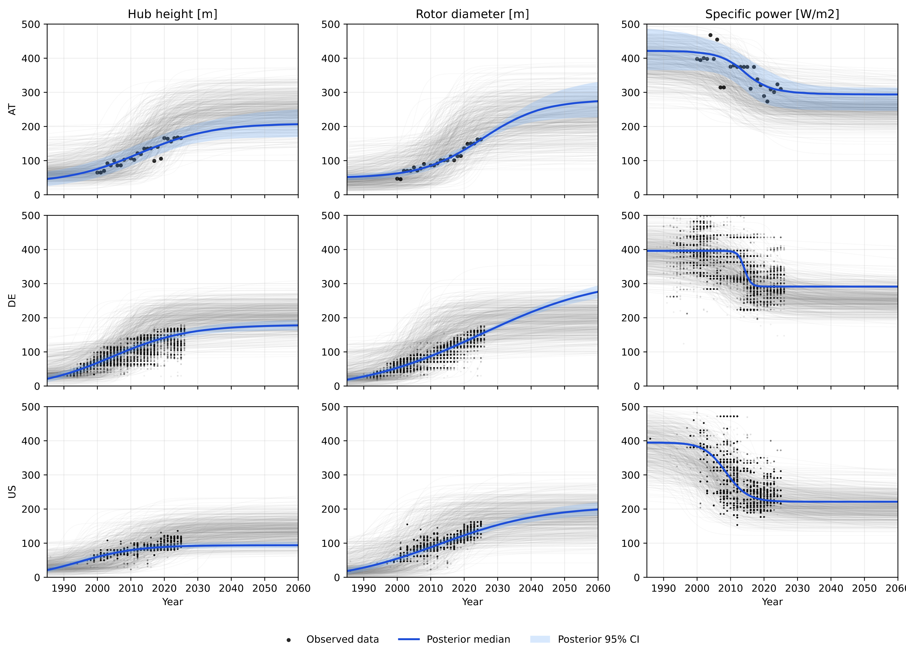
Several patterns emerge from the multi-region comparison. First, hub heights diverge markedly between European and US markets: the Austrian and German median projections for 2055 (204 m and 177 m, respectively) exceed the US projection (94 m) by a factor of approximately two, reflecting persistent regulatory and market-structural differences. Second, specific power projections for Germany and the United States show near-complete saturation by 2030, with negligible further decline to 2055 (DE: $291\to 291$ W/m²; US: $222\to 222$). Austria exhibits a slight residual decline ($300\to 297$ W/m²), consistent with its later market maturity. Third, rotor diameters continue to grow in all regions, driving the increase in derived capacity from 4.1 to 8.7 MW in 2030 to 6.6–16.9 MW in 2055, with the widest credible intervals for Austria reflecting its shorter data record.

The credible-interval widths (see Figure 5) provide a direct measure of projection confidence. For 2030 (5 years ahead), the 95% CI for hub height spans 14 m (AT), 5 m (DE), and 2 m (US), scaling inversely with dataset size. For 2055 (30 years ahead), these intervals widen to 46 m (AT), 13 m (DE), and 3 m (US), illustrating how uncertainty compounds over longer projection horizons and is most pronounced for data-sparse regions.

4.2. Benchmark Comparison

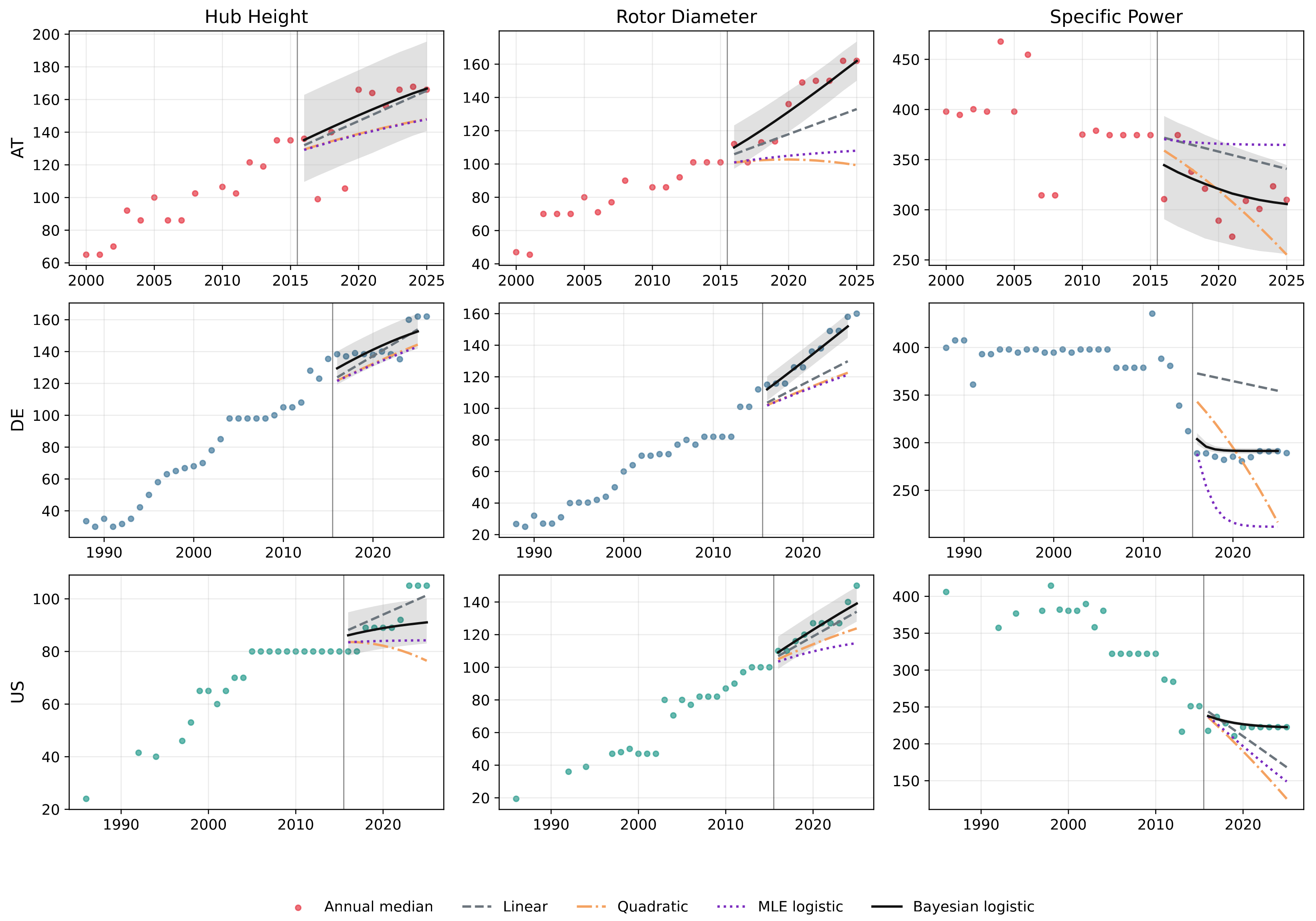
Figure 6 presents the hindcast validation results for the 2015 training cutoff. The Bayesian logistic model consistently tracks post-2015 observations most closely, particularly for metrics approaching saturation (DE and US hub height, all regions’ specific power). The linear model extrapolates without bound, producing physically implausible projections (e.g., US specific power declining below 100 W/m² by 2030). The quadratic polynomial suffers from instability in the extrapolation region, with curvature artifacts producing non-monotonic projections. The MLE logistic model performs comparably to the Bayesian version for data-rich regions (DE, US) but fails to converge or produces extreme estimates for Austria, where the saturation level is not identified by the data alone. All benchmark models were fitted on the same stratified subsample used for the Bayesian fits (N = 5000 for DE and US) to ensure a fair comparison.

Table 6. Hindcast validation metrics (2015 split, test period 2016–2025). Bold indicates best RMSE per region–metric combination. CRPS and coverage are reported only for the Bayesian model.

Region	Metric	Model	RMSE	MAE	CRPS	95% Cov.
AT	Hub Height	Linear	24.3	17.0	—	—
		Quadratic	25.5	20.8	—	—
		MLE Logistic	25.5	21.0	—	—
		Bayesian Logistic	25.3	16.6	13.2	91.1%
AT	Rotor Diam.	Linear	25.4	21.4	—	—
		Quadratic	44.5	37.7	—	—
		MLE Logistic	39.8	33.7	—	—
		Bayesian Logistic	17.9	13.5	9.7	91.8%
AT	Spec. Power	Linear	60.3	46.1	—	—
		Quadratic	62.1	47.1	—	—
		MLE Logistic	67.9	56.2	—	—
		Bayesian Logistic	52.3	34.6	27.3	97.3%
DE	Hub Height	Quadratic	24.8	21.3	—	—
		Linear	25.1	20.3	—	—
		MLE Logistic	24.8	21.4	—	—
		Bayesian Logistic	24.8	19.6	13.9	89.9%
DE	Rotor Diam.	Linear	21.1	17.8	—	—
		Quadratic	23.9	20.5	—	—
		MLE Logistic	24.5	21.0	—	—
		Bayesian Logistic	17.0	12.0	9.0	90.8%
DE	Spec. Power	Bayesian Logistic	63.2	43.8	32.3	95.0%
		Quadratic	76.4	61.0	—	—
		Linear	87.1	75.9	—	—
		MLE Logistic	94.2	75.0	—	—
US	Hub Height	Linear	10.0	8.4	—	—
		Bayesian Logistic	10.8	7.5	5.8	89.2%
		MLE Logistic	13.2	9.5	—	—
		Quadratic	15.2	11.0	—	—
US	Rotor Diam.	Bayesian Logistic	10.8	8.1	6.0	96.0%
		Linear	11.6	8.5	—	—
		Quadratic	14.5	11.2	—	—
		MLE Logistic	17.9	14.6	—	—
US	Spec. Power	Bayesian Logistic	28.4	21.3	15.7	98.6%
		Linear	37.9	29.6	—	—
		MLE Logistic	46.3	36.2	—	—
		Quadratic	53.6	42.0	—	—

reports quantitative hindcast metrics for the 2015 split. The Bayesian logistic model achieves the lowest RMSE in six of nine combinations (linear wins AT-HH and US-HH; quadratic ties DE-HH) and is within 1% of the best in the remaining three, with its advantage most pronounced for rotor diameter (AT: 17.9 vs. 25.4 for linear, 39.8 for MLE logistic) where saturation constraints prevent the overshoot that afflicts unconstrained models.

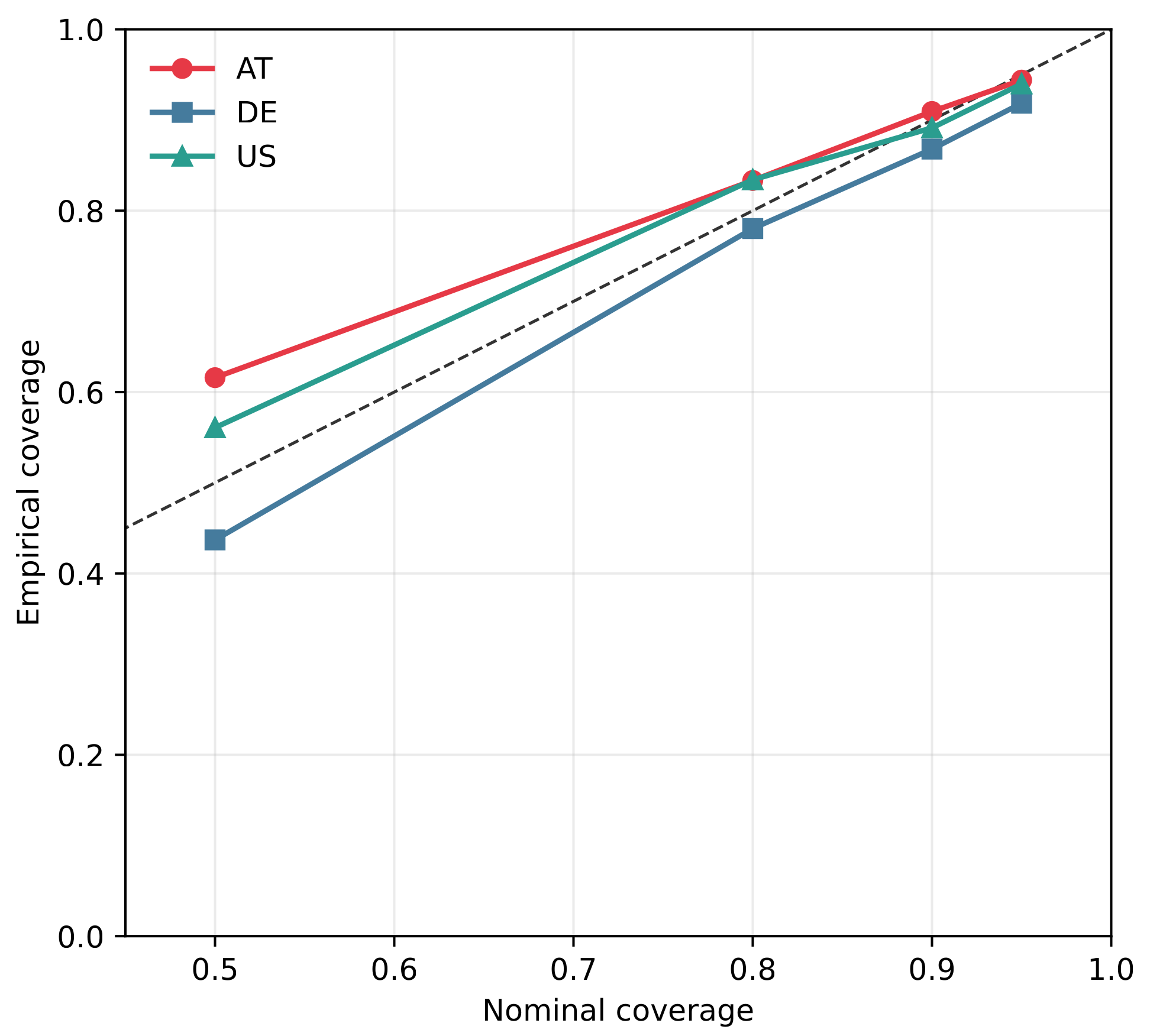
Figure 7 shows the calibration of the Bayesian credible intervals. A perfectly calibrated model would follow the diagonal. All three regions exhibit slight overcover at narrow confidence levels (50% and 80%), indicating conservative uncertainty estimates. At the 95% level, coverage ranges from 91% (AT, DE) to 95% (US), demonstrating well-calibrated uncertainty quantification. The slight conservatism at narrower levels is attributable to the Student-t likelihood, which produces heavier tails than a Gaussian model and thus wider intervals, a deliberate modeling choice that prioritizes robustness over sharpness.

4.3. Prior Sensitivity

Table 7. Prior sensitivity analysis: maximum relative deviation (%) in posterior medians for 2055 projections across the three prior configurations. Values exceeding 10% are highlighted.

Region–Metric	Max. Rel. Deviation [%]	Max. Abs. Deviation	Assessment
AT Hub Height	9.7	—	Borderline
AT Rotor Diameter	20.2	54.8 m	Prior-sensitive
AT Specific Power	4.7	—	Robust
DE Hub Height	4.4	—	Robust
DE Rotor Diameter	11.2	27.3 m	Prior-sensitive
DE Specific Power	0.7	—	Very robust
US Hub Height	8.9	—	Borderline
US Rotor Diameter	13.1	27.2 m	Prior-sensitive
US Specific Power	0.1	—	Very robust

summarizes the maximum relative deviation in posterior medians across the three prior sets (informative, weakly informative, and diffuse) for the 2055 projections.

The results reveal a clear pattern: rotor diameter projections are prior-sensitive across all three regions, while specific power projections are uniformly robust. Hub height occupies an intermediate position, with borderline sensitivity for Austria and the US.

This pattern is physically explainable: specific power has already reached or nearly reached its market-driven saturation level in all three regions (Section 4.1), indicating that the data strongly constrain the posterior regardless of the prior. Rotor diameter, by contrast, is still in the active growth phase in all markets, and its ultimate saturation level is not yet observationally identified—precisely the condition under which prior information becomes influential. The Austrian dataset ($N=534$, 25 years) shows the highest sensitivity (20.2% for rotor diameter), confirming that smaller datasets amplify prior influence.

Notably, the diffuse prior set C caused MCMC divergences for three combinations (AT specific power, DE rotor diameter, and US hub height), indicating that the posterior geometry becomes pathological without informative regularization. This finding supports the use of physically motivated priors not merely as a convenience but as a modeling necessity for logistic curve fitting with finite data.

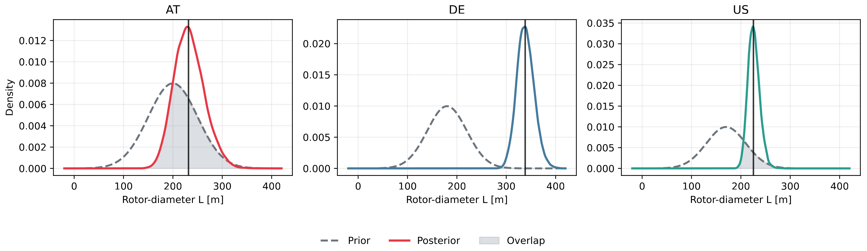
To make the degree of learning explicit, Figure A3 (Appendix E) compares the prior and posterior densities of the rotor-diameter carrying capacity L and quantifies their overlap. For Austria the prior–posterior overlap is large (0.63): with a short, small record the data shift the carrying-capacity estimate only modestly (posterior median 231.6 m versus prior mean 200 m). For Germany the overlap is essentially zero (0.004): the posterior (median 338.3 m, 95% CI 306.5–375.5 m) is far narrower than and strongly shifted above the prior, so the data dominate. The United States is intermediate (overlap 0.21; posterior median 225.4 m). This mirrors the data-richness gradient seen in the prior sensitivity analysis: data-rich regions constrain the posterior strongly, while Austria remains more prior-influenced.

4.4. Climate-Aware Energy Yield

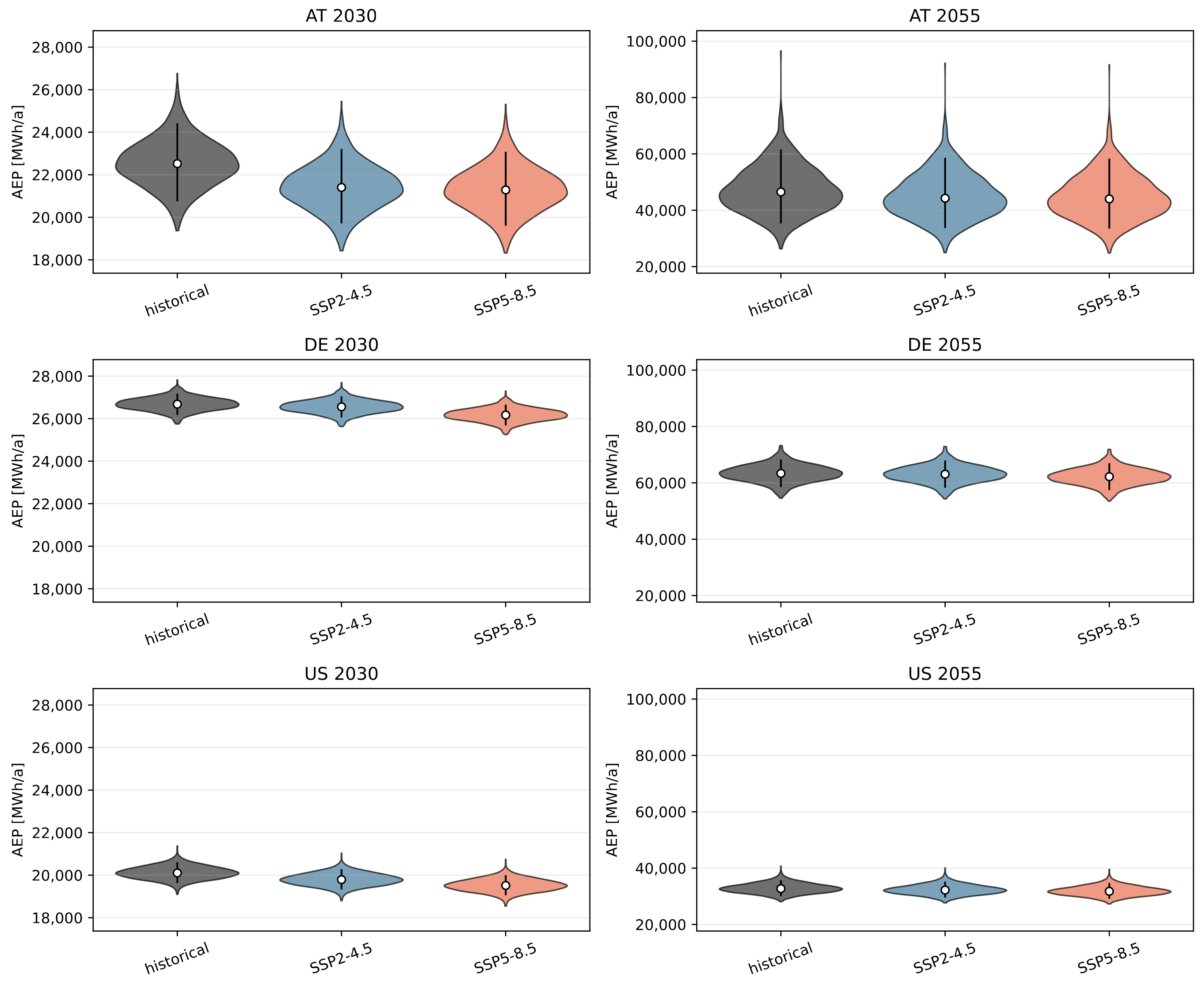
Figure 8 presents the probabilistic annual energy production (AEP) distributions for all region–year–scenario combinations.

Table 8. Probabilistic annual energy production estimates (median, 5th–95th percentile) for a typical turbine at each reference site in three climate simulations. Wind-profile extrapolation uses the site-specific power-law exponents of Table 3 (AT $\alpha =0.227$, DE $\alpha =0.233$, US $\alpha =0.186$); the fixed $\alpha =0.143$ case is reported as a sensitivity comparison in Section 5.7.

Region	Year	Simulation	CF (Median)	AEP [GWh/a]	P5–P95 [GWh/a]
AT	2030	Historical	0.295	22.5	20.7–24.4
AT	2030	SSP2-4.5	0.280	21.4	19.7–23.2
AT	2030	SSP5-8.5	0.278	21.3	19.6–23.1
AT	2055	Historical	0.314	46.5	35.3–61.6
AT	2055	SSP2-4.5	0.299	44.3	33.7–58.6
AT	2055	SSP5-8.5	0.298	44.0	33.5–58.3
DE	2030	Historical	0.437	26.7	26.2–27.2
DE	2030	SSP2-4.5	0.435	26.6	26.1–27.0
DE	2030	SSP5-8.5	0.429	26.2	25.7–26.7
DE	2055	Historical	0.452	63.4	58.5–68.2
DE	2055	SSP2-4.5	0.450	63.1	58.2–67.9
DE	2055	SSP5-8.5	0.444	62.2	57.4–67.0
US	2030	Historical	0.560	20.1	19.6–20.6
US	2030	SSP2-4.5	0.551	19.8	19.3–20.3
US	2030	SSP5-8.5	0.544	19.5	19.1–20.0
US	2055	Historical	0.563	32.7	30.0–35.7
US	2055	SSP2-4.5	0.554	32.2	29.6–35.2
US	2055	SSP5-8.5	0.546	31.8	29.2–34.7

reports the corresponding median values with 5th–95th percentile ranges.

The capacity factors reflect the contrasting wind resources and turbine designs across regions: the US reference site (Nebraska, Great Plains) achieves the highest capacity factors ($\mathrm{CF}\approx$ 0.56), followed by Germany (≈0.45) and Austria (≈0.30). The US advantage arises from both stronger wind resources (Weibull $A=9.0$ m/s vs. 5.8 m/s for AT) and lower specific power (222 vs. 300 W/m²), which increases the ratio of energy captured to rated capacity. The Austrian capacity factor of 0.295 at the Weinviertel reference site corresponds to approximately 2580 full-load hours, which is above the APG grid development plan assumption of ≈2000 FLH [8]. This reflects the above-average wind conditions at the selected reference site; the APG target represents a fleet average across all Austrian sites, including less favorable locations.

Adopting site-specific power-law exponents in place of the generic $1/7$ law materially increases the projected energy yield in the two high-shear European regions while leaving the US essentially unchanged. For 2055 the median AEP rises by $+12.1\%$ (Austria) and $+8.6\%$ (Germany) but falls marginally by $-0.3\%$ for the United States. The US behavior is instructive: although its site exponent ($0.186$) exceeds $0.143$, the projected 2055 US hub height (≈94 m) lies just below the 100 m Weibull reference height, so a larger exponent slightly reduces the extrapolated scale rather than increasing it.

Climate change shifts AEP downward across all regions and simulations, consistent with the slight reductions in Weibull scale parameters projected by GOWIRES. The shift from historical to SSP5-8.5 reduces median AEP by 3–6% in 2030 and 2–5% in 2055, with Austria showing the largest relative sensitivity due to its weaker baseline wind resource.

Uncertainty Decomposition

We decompose the total AEP variance using two complementary approaches. The simulation-based decomposition measures climate uncertainty as the spread across the three scenario endpoints (historical, SSP2-4.5, SSP5-8.5), while technology is varied across posterior samples. The GCM-ensemble decomposition measures climate uncertainty as the inter-model spread across all 13 CMIP6 global climate models within a single SSP pathway, which captures model structural uncertainty in addition to the forced signal.

Table 9. Variance decomposition of projected AEP for 2055 under two uncertainty quantification approaches. The simulation-based approach uses the spread across three SSP endpoints; the GCM-ensemble approach uses the inter-model spread across 13 CMIP6 models within SSP2-4.5. The technology–climate interaction term accounts for less than 0.5% of total variance in all region–simulation combinations and is omitted for clarity.

	Simulation-Based (3 SSPs)		GCM Ensemble (13 Models, SSP2-4.5)
Region	Technology	Climate	Technology	Climate
AT	97.4%	2.6%	85.7%	14.3%
DE	96.0%	4.0%	44.2%	55.8%
US	93.1%	6.9%	73.5%	26.5%

reports both.

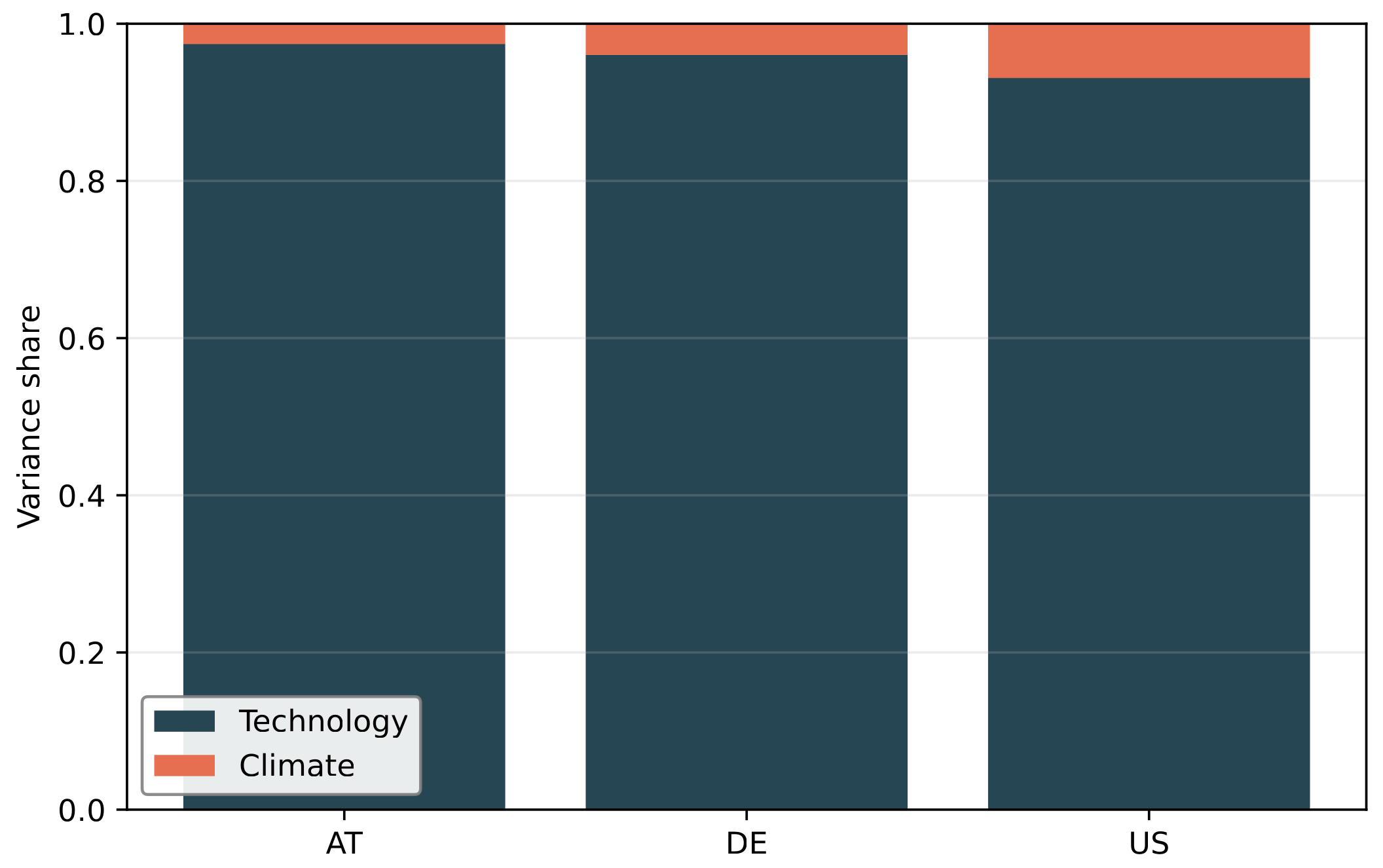
Under the simulation-based approach (Figure 9), technology uncertainty dominates across all regions (93–97%), with climate contributing only 3–7%. This result primarily reflects that the inter-scenario spread in Weibull parameters is small: SSP2-4.5 and SSP5-8.5 produce similar wind resource projections for the 2030–2059 period, consistent with the well-known finding that SSP pathways diverge primarily after mid-century [18].

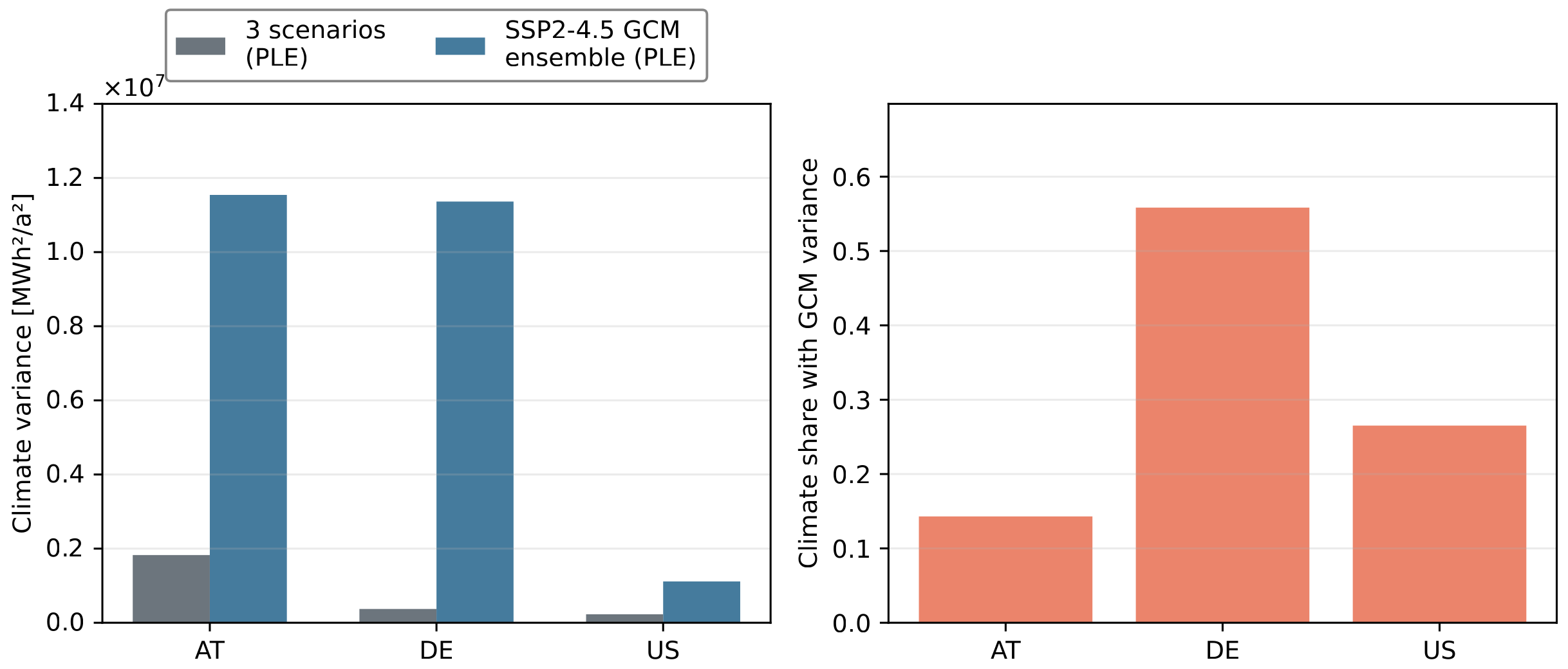
However, when climate uncertainty is measured by the inter-GCM spread within SSP2-4.5, capturing model structural uncertainty in wind projections, the picture changes substantially (Figure 10). For Austria, technology uncertainty remains dominant (≈86%), but climate uncertainty rises from ≈3% to ≈14%. For the US, the shift is also substantial: climate uncertainty rises from ≈7% to ≈26%, reflecting the narrower technology posteriors obtained with the larger subsample. For Germany, the shift is dramatic: climate uncertainty accounts for ≈56% of total variance, exceeding technology uncertainty. This reflects two converging factors: (i) the German technology posteriors are narrow (mature market, N = 5000), leaving less technology variance to dominate, and (ii) the Schleswig-Holstein reference site lies at the boundary between the North Atlantic westerly regime and continental influences, a transition zone where CMIP6 models disagree about the magnitude and sign of future changes in the North Atlantic Oscillation and associated wind speed trends, producing high inter-model spread.

This contrast carries a key methodological message: the relative importance of technology versus climate uncertainty depends critically on how climate uncertainty is quantified. Simulation-based assessments that use only SSP endpoints systematically underestimate climate uncertainty by conflating inter-simulation spread (small for wind) with the full model structural uncertainty (large). Energy system planners should use the full GCM ensemble, where available.

A sensitivity test comparing index-matched versus independently shuffled posterior samples for the German reference site yielded an AEP variance difference of approximately 1.5% ($8.99$ vs. $9.12\times {10}^6$ MWh²/a²), with near-identical medians, confirming that the cross-metric correlation structure has negligible impact on the uncertainty estimates.

5. Discussion

5.1. Regional Projections in Context

Table 10. Comparison of Bayesian posterior medians (95% CI) with institutional projections for 2030.

Metric	AT	DE	US	IEA Task 26 “Likely”	NREL ATB (T2–T3)
Hub height [m]	179 (172–186)	162 (159–164)	93 (92–94)	125	—
Rotor diam. [m]	192 (184–201)	175 (173–176)	153 (151–156)	—	148–196
Spec. power [W/m2]	300 (280–316)	291 (288–294)	222 (220–224)	250	192–275
Capacity [MW]	8.7 (7.8–9.7)	7.0 (6.8–7.1)	4.1 (4.0–4.2)	—	3.3–8.3

places our 2030 projections alongside institutional benchmarks. The Austrian specific power projection of ≈300 W/m² aligns closely with both the APG grid development plan (≈300 W/m², ≈2000 full-load hours [8]) and the current German market average of 302 W/m², reflecting the topographic and regulatory constraints of Alpine and Central European markets. The German projection of 292 W/m² is similarly consistent with the NEP reference turbine (≈308 W/m² [7]). Both European projections exceed the IEA Wind TCP Task 26 “likely” scenario of 250 W/m² for 2030 [3], suggesting that the observed European market trajectory is more conservative than expert expectations, a finding that our data-driven framework captures by design.

The US projection of 222 W/m² falls within the NREL ATB corridor (192–275 W/m² [4]) but is conservative relative to the technology frontier classes (T3: 192 W/m²), capturing the fleet average rather than best-available technology. This is consistent with the framework’s role as a market-trajectory tool: it projects what is being deployed, not what could be deployed with frontier technology.

Hub height projections reveal the most striking regional divergence. The European markets project continued growth toward 177–204 m by 2055, while the US appears to saturate near 94 m. This 80–110 m gap reflects fundamental differences in regulatory environments (US height restrictions and European permitting for taller structures), land economics (abundant low-cost land in the US reduces the incentive for taller towers), and wind resource characteristics (the US Great Plains offer strong winds at relatively low heights). For energy system planners, this implies that uniform global assumptions about future turbine dimensions, which are common in integrated assessment models, may introduce systematic biases.

We note that institutional values (IEA scenarios, NREL ATB classes, and NEP reference turbines) represent planning targets or scenario assumptions rather than empirical projections; our posterior medians capture observed market trajectories. The comparison illustrates alignment in magnitude, not methodological equivalence.

5.2. Methodological Strengths

The benchmark comparison (Section 4.2) demonstrates three specific advantages of the Bayesian logistic approach over simpler alternatives.

First, the physical saturation constraint prevents the unbounded extrapolation that afflicts linear and polynomial models. This advantage is most visible for rotor diameter, where the Bayesian model achieves RMSE improvements of 30–55% over the linear baseline for all three regions.

Second, Bayesian regularization via informative priors stabilizes the fit where maximum-likelihood estimation fails. The MLE logistic model produced extreme or non-convergent estimates for Austria, where 25 years of data in the exponential growth phase cannot identify the saturation level. The Bayesian framework resolves this identifiability problem by anchoring the carrying capacity through physically motivated priors, yielding plausible projections even for data-sparse markets.

Third, the probabilistic output provides calibrated uncertainty quantification. The empirical coverage of the 95% credible interval ranges from 91% to 97% across regions and metrics (Figure 7), indicating slight conservatism, a desirable property for planning applications where underestimation of uncertainty carries greater risk than overestimation. The Student-t likelihood contributes to this conservatism through heavier tails than a Gaussian model, a deliberate trade-off favoring robustness over sharpness.

5.3. Prior Sensitivity and the Role of Expert Knowledge

The prior sensitivity analysis (Section 4.3) reveals a systematic pattern: specific power projections are uniformly robust across all prior configurations (maximum deviation < 5%), while rotor diameter projections are prior-sensitive in all three regions (11–20% deviation). This pattern has a clear physical interpretation. Specific power has already reached or approached its market-driven saturation floor, meaning the data strongly constrain the posterior. Rotor diameter remains in its active growth phase, and the ultimate saturation level is not yet observationally identified—the condition under which Bayesian priors become influential.

This finding has practical implications for framework users. For metrics where the data are informative (specific power in mature markets, hub height for data-rich regions), the framework delivers data-driven projections that are robust to prior specification. For metrics still in the growth phase (rotor diameter universally, hub height in small markets), the prior encodes a consequential assumption about the physical upper bound. Users should therefore invest particular care in specifying rotor diameter priors, ideally drawing on engineering assessments of transport constraints, structural limits, and regulatory tip-height ceilings.

The observation that diffuse priors caused MCMC divergences for three region–metric combinations further supports the use of informative priors not merely as a convenience but as a modeling necessity. Without physical regularization, the posterior geometry of logistic models with finite data becomes pathological, confirming that the Bayesian framework is not simply “adding assumptions” but rather encoding essential structural knowledge that the data alone cannot provide.

5.4. Interpretation of Specific Power Saturation

A notable feature of our results is that the specific power projections for Germany and the United States show near-complete saturation by 2030, with negligible further decline projected to 2055 (DE: $291\to 291$ W/m²; US: $222\to 222$ W/m²). This does not imply that turbine technology has reached its physical limits: the NREL Big Adaptive Rotor project targets 150 W/m² and DTU’s LowWind project has demonstrated designs at 100 W/m² [4]. Rather, it reflects that the observed market trajectory has not yet incorporated these frontier technologies at scale.

As meteorologists and energy system analysts rather than turbine engineers, we deliberately position this framework as a tool that honestly reports what the data show, while offering a structured interface through Bayesian priors for technology experts to inject knowledge about anticipated breakthroughs. For instance, setting the specific power lower bound $y_{min}$ to 180 W/m² based on engineering assessments would yield steeper projected declines that reflect anticipated innovation rather than observed market behavior. This separation of data-driven inference from expert judgment is a methodological strength: it makes explicit where projections are driven by evidence and where they depend on assumptions. We distinguish three mechanisms that can produce observed specific power saturation: physical limits (engineering constraints on rotor scaling), economic saturation (diminishing LCOE returns below ≈200 W/m² as documented by Bolinger et al. [20]), and regulatory saturation (tip-height restrictions that constrain rotor diameter for a given hub height). The observed market saturation in our data likely reflects the latter two factors rather than fundamental physical limits, which is precisely why the configurable $y_{min}$ prior allows users to distinguish between “what the market does” and “what engineering permits.”

5.5. Technology Versus Climate Uncertainty

The variance decomposition reveals that the relative importance of technology versus climate uncertainty is not a fixed property but depends on three factors: the maturity of the wind market (which determines the width of technology posteriors), the climate sensitivity of the reference site (which determines inter-GCM spread), and the method of uncertainty quantification (scenario endpoints versus full GCM ensemble).

Under the simulation-based approach, technology uncertainty dominates for all regions (93–97%), consistent with Pryor and Barthelmie’s [18] observation that inter-scenario differences in wind resources are small through mid-century. However, the GCM-ensemble decomposition shows that for mature markets with narrow technology posteriors (Germany), inter-model climate uncertainty can dominate (≈56%), while for emerging markets with wide technology posteriors (Austria) or sites with low inter-GCM disagreement (US), technology remains the primary source.

This finding carries two practical messages. First, for emerging wind markets and near-term planning horizons (2030), investment in reducing technology projection uncertainty, through better data, more refined models, or targeted expert elicitation, yields the greatest returns in planning confidence. Second, for mature markets and longer horizons (2055), the full GCM ensemble spread should be propagated through the energy yield chain, as simulation-based assessments underestimate climate uncertainty by an order of magnitude. Our framework, by producing technology posteriors that can be combined with arbitrary climate ensembles, provides the infrastructure for both applications.

5.6. The Probabilistic Gap in Energy System Planning

Our results highlight what we term the “probabilistic gap” in current energy system planning practice. Transmission system operators increasingly employ probabilistic adequacy methods (Section 1.1), yet their underlying turbine technology assumptions remain deterministic point estimates [6,7,8].

Our framework directly addresses this gap. The posterior distributions for hub height, rotor diameter, specific power, and derived capacity can serve as probabilistic inputs to the same Monte Carlo frameworks that already handle demand and weather uncertainty. The open-source pipeline is designed to produce outputs in formats compatible with standard energy system modeling workflows.

5.7. Limitations

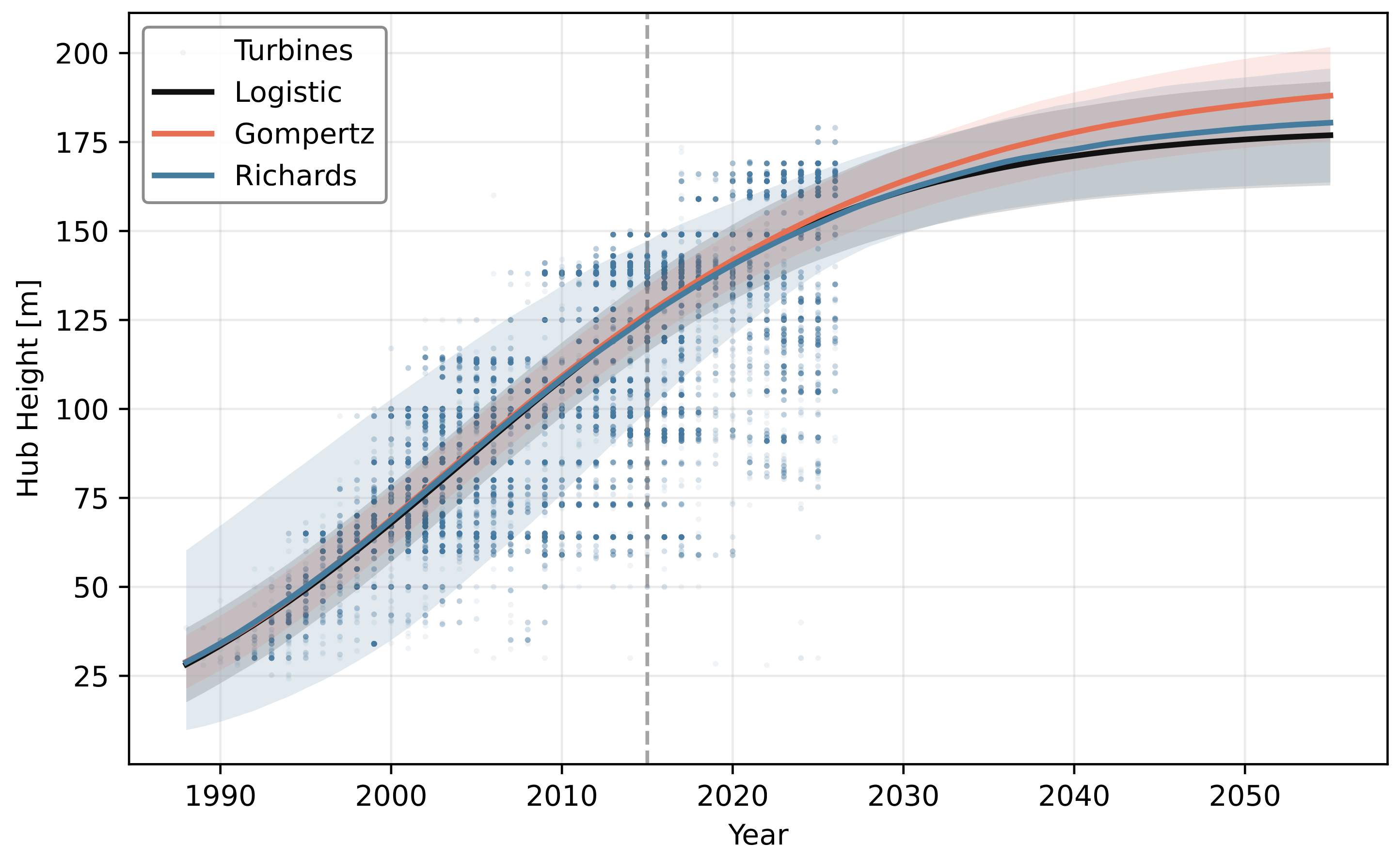
Several limitations should be noted. First, the framework uses the standard four-parameter logistic for interpretability and physical transparency. To test whether this is restrictive, we compared the logistic, Gompertz, and Richards forms for German hub height (Appendix D). The three forms are statistically indistinguishable (the maximum elpd difference, ≈6, is far below its standard error of ≈68) and agree to within 2.1 m for 2030; the 2055 medians spread by up to 10.5 m with overlapping 95% credible intervals (Gompertz highest at 187.7 m and logistic lowest at 177.2 m). Long-horizon extrapolation therefore carries a genuine but bounded functional-form uncertainty, consistent with Zielonka et al. [9], who found generalized Richards and Bertalanffy formulations advantageous in technology-diffusion forecasting. Extending to asymmetric or regime-switching growth models is a natural direction for future work.

Second, the framework assumes a single continuous S-curve per metric and region, with no mechanism for modeling discrete technology jumps (e.g., the introduction of segmented blades or superconducting generators) or policy shocks (e.g., sudden changes in height restrictions or subsidy structures). Such discontinuities would manifest as deviations from the fitted trend and could be addressed through change-point models or regime-switching extensions.

Third, lower specific power increases capacity factors and reduces output variability, enhancing the system value of wind generation [20]. However, this comes at the cost of deliberate energy curtailment (“spilling”) at high wind speeds, a trade-off that our current energy yield framework does not explicitly model. Incorporating curtailment losses and their economic implications would require coupling with market or dispatch models.

Fourth, the cross-metric uncertainty propagation uses index-matched posterior samples rather than a joint multivariate Bayesian model, capturing temporal correlations but not structural dependencies between turbine dimensions. A hierarchical model jointly estimating hub height, rotor diameter, and specific power, potentially with cross-regional partial pooling, would provide a more principled treatment of these dependencies.

Fifth, the synthetic power curve parameterization following Ryberg et al. [17] is a simplified representation that does not capture manufacturer-specific design variations, site-specific derating, or wake effects. For applications requiring higher fidelity, the framework’s posterior outputs can be coupled with more detailed power curve models.

Sixth, the wind-profile extrapolation uses a single region-representative shear exponent per region (Table 3) rather than a time-varying, stability-resolved, or turbine-site-specific profile. Relative to the generic $\alpha =0.143$ law, the region-representative exponents change the 2055 median AEP by $+12.1\%$ (AT), $+8.6\%$ (DE), and $-0.3\%$ (US). A broader sensitivity sweep ($\alpha$ from 0.10 to 0.20) changes median AEP by up to ≈14% for Austria (projected 2055 hub height 204 m) but by less than 1% for the US (projected 2055 hub height ≈ 94 m), where the small hub-height-to-reference-height ratio renders the extrapolation nearly insensitive to $\alpha$. These exponents are a clear improvement over the universal $1/7$ value but remain single representatives per region; an operational single-site resource assessment would require locally measured or mesoscale-modeled shear profiles. Alternative extrapolation approaches, including logarithmic profiles, stability-corrected methods, or mesoscale-model-derived wind climatologies, may be more appropriate depending on terrain complexity, particularly for Alpine sites (Austria) where thermal circulations and channeling effects render power-law extrapolation least reliable.

Seventh, the Austrian dataset (534 of ≈1400 commissioned turbines) exhibits higher coverage for recent installations, potentially introducing a selection bias toward well-documented modern turbines. The elevated Austrian specific power values (median 323 W/m² in 2024 vs. ≈270 W/m² for the European average reported by WindEurope [25]) are consistent with this selection effect and with the regulatory and topographic constraints of Austrian Alpine and sub-Alpine sites, but the magnitude of any bias cannot be quantified without access to the complete installation register.

Eighth, the assumption that wind speeds remain Weibull-distributed under future climate conditions has not been verified for the reference sites. Changes in atmospheric stability regimes or mesoscale circulation patterns could alter the distributional shape, introducing an additional source of structural uncertainty not captured in the current framework.

Ninth, the production fits for the two large datasets rely on a single stratified N = 5000 subsample. A five-subsample robustness check (Appendix A) now spans all three technology metrics for Germany and the United States. All 30 refits converged cleanly ($\widehat{R}=1.000$, zero divergences; ESS_min = 6509), and the direction and order of magnitude of the projections are stable across independent subsamples. The spread of subsample medians remains non-negligible relative to the conditional posterior interval, with SD/CI ratios of 0.33–0.57 for hub height and 0.10–0.42 for rotor diameter and specific power. The single-subsample posterior interval thus understates total uncertainty by this subsample-selection component, which we report as a supplementary diagnostic.

5.8. Transferability and Future Work

The framework is designed for transferability. Any market with public turbine installation records containing commissioning year, hub height, rotor diameter, and rated capacity can serve as input. Particularly promising candidates include Denmark, whose turbine register extends back to the 1970s and would provide the only complete S-curve observation (lag phase through saturation), the United Kingdom (≈12,000 turbines via REPD), and the Nordic markets. The GOWIRES dataset [14], with 416,417 turbines across 89 countries, provides a ready-made data source for global application.

Several extensions are planned. First, hierarchical Bayesian models with partial pooling across regions could share information between data-rich and data-poor markets, improving projections for emerging wind markets. Second, the prior specification could be formalized as an interactive elicitation protocol, enabling systematic integration of stakeholder knowledge. Third, coupling the turbine projections with spatial optimization models would enable probabilistic assessments of future wind energy potential at the landscape scale, extending the approach of Ryberg et al. [17] to a fully probabilistic framework.

6. Conclusions

We presented a Bayesian logistic framework for probabilistic wind turbine technology projections, validated across three major onshore wind markets with over 103,000 turbines spanning four decades. The key findings are:

• Plausible, well-calibrated projections: The framework produces turbine characteristic projections that align with institutional benchmarks (IEA, NREL, ENTSO-E, and national grid development plans) while providing formal uncertainty quantification absent from existing planning tools. The 95% credible intervals achieve 91–97% empirical coverage in hindcast validation.
• Superior hindcast performance: The Bayesian logistic model outperforms linear, polynomial, and maximum-likelihood logistic alternatives in six of nine region–metric combinations, with the largest improvements for rotor diameter where physical saturation constraints prevent the extrapolation overshoot of unconstrained models.
• Transparent prior influence: The prior sensitivity analysis reveals that specific power projections are data-driven and robust (<5% sensitivity) across all regions, while rotor diameter projections depend meaningfully on prior specification (11–20% sensitivity), identifying exactly where expert knowledge is essential and where the data speak for themselves.
• Uncertainty dominance is method- and region-dependent: Under simulation-based decomposition conditions (three SSP endpoints), technology uncertainty dominates (93–97%). However, when the full inter-model spread across 13 CMIP6 global climate models is propagated, climate uncertainty rises to 14% (Austria), 26% (US), and 56% (Germany), demonstrating that the commonly reported “technology dominates” finding is sensitive to how climate uncertainty is quantified. For emerging markets with wide technology posteriors, reducing technology uncertainty yields the greatest planning benefit; for mature markets, the full GCM ensemble must be considered.
• A baseline tool for the energy planning community: The framework is explicitly positioned as a data-driven baseline that captures observed market trajectories. It does not predict engineering breakthroughs. But through configurable Bayesian priors, it offers a principled interface for technology experts to encode anticipated innovations, making the boundary between evidence and assumption transparent and auditable.

The open-source analysis pipeline, designed for reproducibility and direct adoption, is available at https://github.com/ischicker/bayesian-turbine-projections (accessed on 21 June 2026). We invite the energy modeling community to apply the framework to additional markets, extend it to offshore wind and solar PV, and integrate its probabilistic outputs into the Monte Carlo workflows that increasingly underpin energy system adequacy assessments.

References

1. Wiser, R.; Rand, J.; Seel, J.; Beiter, P.; Baker, E.; Lantz, E.; Gilman, P. Expert elicitation survey predicts 37% to 49% declines in wind energy costs by 2050. Nat. Energy 2021, 6, 555–565. [Google Scholar] [CrossRef]
2. Beiter, P.; Cooperman, A.; Lantz, E.; Stehly, T.; Shields, M.; Wiser, R.; Telsnig, T.; Kitzing, L.; Berber, V.; Hainsch, K. Wind power costs driven by innovation and experience with further reductions on the horizon. Wiley Interdiscip. Rev. Energy Environ. 2022, 11, e398. [Google Scholar]
3. IEAWind TCP Task 26. Cost of Wind Energy. Available online: https://iea-wind.org/task26/ (accessed on 14 May 2026).
4. National Renewable Energy Laboratory. Annual Technology Baseline (ATB). 2024. Available online: https://data.openei.org/submissions/6006 (accessed on 14 May 2026).
5. International Renewable Energy Agency. Future of Wind: Deployment, Investment, Technology, Grid Integration and Socio-Economic Aspects; IRENA: Abu Dhabi, United Arab Emirates, 2019. [Google Scholar]
6. ENTSO-E. European Resource Adequacy Assessment (ERAA) 2024, Executive Report; ENTSO-E: Brussels, Belgium, 2024. [Google Scholar]
7. 50Hertz; Amprion; TenneT; TransnetBW. Netzentwicklungsplan Strom 2037/2045, Version 2025; German TSOs: Berlin, Germany, 2025. [Google Scholar]
8. Austrian Power Grid. Netzentwicklungsplan 2025; APG: Vienna, Austria, 2025. [Google Scholar]
9. Zielonka, N.; Wen, X.; Trutnevyte, E. Probabilistic projections of granular energy technology diffusion at subnational level. PNAS Nexus 2023, 2, pgad321. [Google Scholar] [CrossRef] [PubMed]
10. Way, R.; Ives, M.C.; Mealy, P.; Farmer, J.D. Empirically grounded technology forecasts and the energy transition. Joule 2022, 6, 2057–2082. [Google Scholar] [CrossRef]
11. Bošnjaković, M.; Katinić, M.; Sánta, R.; Marić, D. Wind Turbine Technology Trends. Appl. Sci. 2022, 12, 8653. [Google Scholar] [CrossRef]
12. Hoen, B.D.; Diffendorfer, J.E.; Rand, J.T.; Kramer, L.A.; Garrity, C.P.; Hunt, H.E. United States Wind Turbine Database V8.3 (March 25, 2026): U.S. Geological Survey, American Clean Power Association, and Lawrence Berkeley National Laboratory Data Release. Various Updates. 2018. Available online: https://data.usgs.gov/datacatalog/data/USGS:57bdfd8fe4b03fd6b7df5ff9 (accessed on 21 June 2026).
13. Bundesnetzagentur. Marktstammdatenregister (MaStR). Available online: https://www.marktstammdatenregister.de/ (accessed on 13 May 2026).
14. Jung, C.; Schindler, D. GOWIRES: A global dataset of onshore wind turbines with site-specific historical and future wind resources. Sci. Data 2026, 13, 290. [Google Scholar]
15. International Renewable Energy Agency. Renewable Power Generation Costs in 2023; IRENA: Abu Dhabi, United Arab Emirates, 2024. [Google Scholar]
16. Gelman, A.; Carlin, J.B.; Stern, H.S.; Dunson, D.B.; Vehtari, A.; Rubin, D.B. Bayesian Data Analysis, 3rd ed.; Chapman and Hall/CRC: Boca Raton, FL, USA, 2013. [Google Scholar]
17. Ryberg, D.S.; Caglayan, D.G.; Schmitt, S.; Linssen, J.; Stolten, D.; Robinius, M. The future of European onshore wind energy potential: Detailed distribution and simulation of advanced turbine designs. Energy 2019, 182, 1222–1238. [Google Scholar] [CrossRef]
18. Pryor, S.C.; Barthelmie, R.J.; Bukovsky, M.S.; Leung, L.R.; Sakaguchi, K. Climate change impacts on wind power generation. Nat. Rev. Earth Environ. 2020, 1, 627–643. [Google Scholar] [CrossRef]
19. Martinez, A.; Iglesias, G. Global wind energy resources decline under climate change. Energy 2024, 288, 129765. [Google Scholar]
20. Bolinger, M.; Lantz, E.; Wiser, R.; Hoen, B.; Rand, J.; Hammond, R. Opportunities for and limitations to further reductions in the specific power rating of wind turbines installed in the United States. Wind Eng. 2021, 45, 351–368. [Google Scholar]
21. Lange, K.L.; Little, R.J.A.; Taylor, J.M.G. Robust Statistical Modeling Using the t Distribution. J. Am. Stat. Assoc. 1989, 84, 881–896. [Google Scholar] [CrossRef]
22. Hoffman, M.D.; Gelman, A. The No-U-Turn Sampler: Adaptively Setting Path Lengths in Hamiltonian Monte Carlo. J. Mach. Learn. Res. 2014, 15, 1593–1623. [Google Scholar]
23. Salvatier, J.; Wiecki, T.V.; Fonnesbeck, C. Probabilistic programming in Python using PyMC3. PeerJ Comput. Sci. 2016, 2, e55. [Google Scholar] [CrossRef]
24. Emeis, S. Wind Energy Meteorology: Atmospheric Physics for Wind Power Generation; Springer: Berlin, Germany, 2013. [Google Scholar]
25. WindEurope. Wind Energy in Europe: 2023 Statistics and the Outlook for 2024–2028; WindEurope: Brussels, Belgium, 2024. [Google Scholar]
Figure 1. Distributional evolution of hub height, rotor diameter, and specific power across decades and regions. Violin width is proportional to sample size. White dots indicate medians; black bars show interquartile ranges.
Energies 19 03009 g001
Figure 2. Annual time series of turbine metrics by region. Austria (left): annual medians with interquartile range bands (light red shadow area) . Germany (center) and United States (right): individual turbine observations (dots) with annual median trend lines.
Energies 19 03009 g002
Figure 3. Annual (top) and cumulative (bottom) number of turbines per region after quality control.
Energies 19 03009 g003
Figure 4. Normalized index trends (2010 = 100) for annual median hub height, rotor diameter, and specific power. Shaded bands indicate interquartile ranges. The normalization enables direct comparison of relative growth and decline rates across regions with vastly different absolute scales and fleet sizes.
Energies 19 03009 g004
Figure 5. Bayesian logistic fits for hub height (left), rotor diameter (center), and specific power (right) across Austria (top), Germany (middle), and the United States (bottom). Solid lines show posterior medians; shaded bands indicate 95% credible intervals. For Austria, annual medians with interquartile ranges are shown instead of individual observations to preserve data confidentiality, dots in the German and United States plots show actual values. The vertical dashed line marks the 2015 hindcast split.
Energies 19 03009 g005
Figure 6. Hindcast validation with 2015 training cutoff. Each panel shows annual median observations (dots) alongside predictions from four models: linear (dashed gray), quadratic (dash-dot orange), MLE logistic (dotted purple), and Bayesian logistic (solid black with 95% CI shading). The vertical line marks the train/test boundary.
Energies 19 03009 g006
Figure 7. Calibration of Bayesian credible intervals averaged across metrics. The dashed diagonal represents perfect calibration. All regions show slight overcover at narrow intervals (conservative behavior) and near-ideal calibration at the 95% level.
Energies 19 03009 g007
Figure 8. Probabilistic annual energy production distributions for 2030 (left) and 2055 (right) in three climate simulations: historical (gray), SSP2-4.5 (blue), and SSP5-8.5 (red). Y-axes are sharedwithin columns to enable cross-regional comparison. White dots indicate medians. The violin widths illustrate that technology uncertainty (spread within each violin) far exceeds simulation-based climate uncertainty (shift between violins); the substantially larger GCM-ensemble climate uncertainty is discussed in the Uncertainty Decomposition Section.
Energies 19 03009 g008
Figure 9. Simulation-based variance decomposition of projected AEP for 2055: technology uncertainty (from Bayesian turbine posteriors) versus climate uncertainty (spread across historical, SSP2-4.5, and SSP5-8.5 simulations).
Energies 19 03009 g009
Figure 10. GCM-ensemble variance decomposition for 2055 under SSP2-4.5. Climate uncertainty is measured as the inter-model spread across 13 CMIP6 global climate models. For Germany, where technology posteriors are narrow and inter-GCM wind disagreement is high, climate uncertainty dominates. In both panels, technology variance is held fixed at the value from the simulation-based decomposition (Table 9); only the climate variance component is recomputed from the GCM ensemble.
Energies 19 03009 g010