A Hybrid Framework for Offshore Wind Power Forecasting: Integration of Adaptive Decomposition and Collaborative Temporal-Channel Modeling

Abstract

Accurate forecasting of offshore wind power is essential for the stability of power systems, yet it remains challenging due to the strong non-stationarity and complex multivariate coupling of meteorological data. To address the tendency of error accumulation in medium- and long-term predictions, this paper proposes a novel framework, termed ISSAVMD-TCN-SOFTS, which integrates adaptive signal decomposition with lightweight deep temporal modeling. Specifically, an improved sparrow search algorithm, enhanced by Lévy flight and sine–cosine modulation mechanisms, is introduced to adaptively optimize the parameters of variational mode decomposition (VMD). This optimization ensures the robust decomposition of highly non-stationary power series. Furthermore, the framework combines the capability of temporal convolutional networks (TCN) to extract multiscale local temporal features with the efficiency of the STAR module in SOFTS for modeling global channel dependencies. Experiments on multi-site, multi-horizon SCADA data from real offshore wind farms show that the proposed model reduces MAE and RMSE by 10–45% compared with mainstream linear models, recurrent neural networks, and Transformer-based models, and maintains high stability over extended forecasting horizons. The results confirm that the integration of adaptive decomposition and collaborative temporal-channel modeling provides an effective solution for the accurate and stable forecasting of offshore wind power.

1. Introduction

The development of clean energy is an essential pathway to achieve carbon neutrality, with offshore wind power emerging as a primary driving force due to abundant resources and proximity to coastal load centers [1,2]. However, the large-scale integration of offshore wind power into the power grid presents substantial challenges. Unlike onshore environments, marine meteorological conditions are highly complex. The power output is heavily influenced by dynamic interactions among multiple environmental factors, resulting in wind speed sequences that exhibit extreme non-stationarity and stochastic volatility [3]. The inability to accurately forecast these fluctuations compromises the stability of the power system and leads to severe wind curtailment.

Despite recent advancements, accurate forecasting continues to face critical structural and algorithmic bottlenecks. First, the direct application of multivariate deep learning models to raw meteorological signals inevitably leads to severe overfitting. While adaptive high-order signal decomposition techniques can mitigate this non-stationarity, the performance of advanced decomposition methods is highly sensitive to parameter selection. Conventional metaheuristic algorithms frequently fail to locate globally optimal parameters, resulting in unstable decomposition [4]. Furthermore, complex dynamic couplings exist among multiple meteorological variables. Existing forecasting architectures struggle to simultaneously model global channel dependencies and local temporal dynamics without introducing disastrous computational overhead. A specialized framework that enforces adaptive noise reduction while efficiently processing high-dimensional channel data is urgently required.

To address these limitations, the objective of this study is to develop a closed-loop forecasting framework, termed ISSAVMD-TCN-SOFTS, that establishes an intrinsic synergy between adaptive signal decomposition and efficient multivariate deep temporal modeling. Specifically, this study aims to answer the following research questions.

• RQ1: How can adaptive optimization strategies be formulated to robustly determine the parameters of signal decomposition, thereby mitigating the risk of local optima and extracting non-stationary dynamic features?
• RQ2: How can deep learning architectures be designed to collaboratively model multi-scale local temporal patterns and global channel dependencies across high-dimensional decomposed data with strictly linear computational complexity?
• RQ3: To what extent does the integration of adaptive decomposition and linear-complexity channel modeling improve the accuracy and stability of offshore wind power forecasting compared to existing mainstream models?

By proposing the ISSAVMD-TCN-SOFTS framework, this study provides a comprehensive solution to these questions. An improved sparrow search algorithm is introduced to adaptively optimize the parameters of variational mode decomposition. To counterbalance the computational overhead, the framework integrates a temporal convolutional network with the SOFTS architecture, which efficiently captures long-term temporal dependencies and global channel interactions.

The remainder of this paper is organized as follows: Section 3 describes the datasets, experimental methods, and platform used for model evaluation, presents the detailed structure of the proposed forecasting model and the methodologies employed in this study. Section 4 reports the simulation results. Section 5 provides comparative analyses. Section 6 reviews the research in this paper. Finally, Section 8 provides the concluding remarks.

2. Research Background

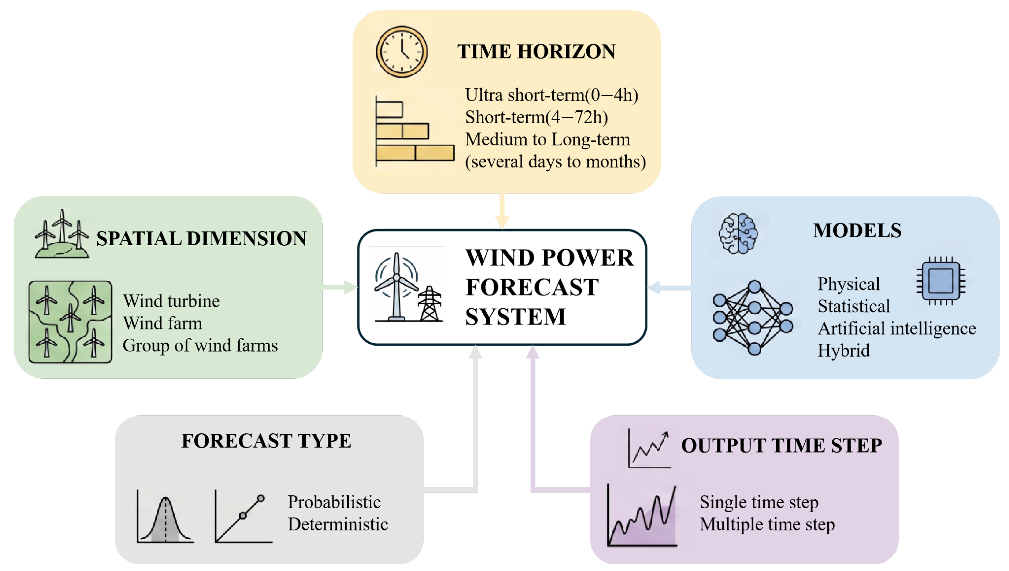
Wind power forecasting models are currently classified based on forecasting conditions and variables, as illustrated in Figure 1. Regarding the time scale, these models fall into three categories: ultra-short-term, short-term, and medium- to long-term forecasting. Specifically, ultra-short-term forecasting typically covers a horizon from minutes up to 4 h (commonly with a temporal resolution of 1–15 min) and focuses on real-time dispatch and integrated control; short-term forecasting generally spans from 4 to 72 h (with a resolution of 15–60 min) and facilitates grid dispatch and the improvement of power quality; while medium- to long-term forecasting extends from several days to months or even years (usually at hourly or daily resolution), primarily supporting the estimation of annual energy production and maintenance planning. Based on the underlying driving mechanisms, forecasting models are typically categorized into physical models, statistical models, machine learning models, and hybrid models. Broadly, these approaches can be consolidated into three primary categories: physical methods, statistical methods, and artificial intelligence-based methods.

Physical methods primarily rely on numerical weather prediction (NWP) data and estimate the power output by establishing atmospheric fluid dynamics equations and power curve models for wind turbines [5]. Although these methods exhibit stable performance in long-term forecasting, they suffer from high computational complexity and a limited capability to capture microscale meteorological phenomena, such as wind shear and turbulence intensity. Consequently, this limitation results in substantial errors in short-term forecasting. Conversely, statistical methods extrapolate future values based on linear patterns within historical time series. However, when applied to the non-stationary and nonlinear “anti-peak-shaving” characteristics of offshore wind power data, conventional linear models frequently fail to capture the underlying dynamic evolution [6].

With the rapid development of data-driven techniques, artificial intelligence methods have become dominant. Early recurrent neural network (RNN)-based models, such as LSTM and GRU, mitigate gradient vanishing via gating mechanisms [7]. For instance, Liu et al. [8] combined LSTM with backpropagation (BP) neural networks to exploit both the temporal learning capability and the advantages of nonlinear fitting, thereby improving forecasting accuracy. Ren et al. [9] integrated convolutional neural networks (CNNs), GRUs, and attention mechanisms to model decomposed wind power signals accurately. However, their sequential computation limits training efficiency and long-sequence modeling capability.

To address this limitation, Bai et al. [10] proposed Temporal Convolutional Networks (TCN), which employ dilated causal convolutions and residual connections to enable parallel computation and enlarge receptive fields. Nguyen et al. [11] further demonstrated superior performance over LSTM in wind forecasting tasks, although long-range dependency modeling remains limited.

Following the success of Transformer [12], self-attention mechanisms have been widely adopted in time series forecasting. Wang et al. [13] proposed a physics-constrained Transformer framework that incorporates wind energy conversion mechanisms into the learning process, thereby improving both forecasting accuracy and physical consistency. Guo et al. [14] developed an uncertainty-aware Transformer model integrating multiscale attention and adaptive feature fusion, which enhances the representation of stochastic fluctuations while providing probabilistic forecasting results. Zhang et al. [15] introduced a Transformer-based framework with spatially adaptive embedding and a meta-feature bank, enabling the extraction of complex spatial correlations among turbines and significantly improving forecasting performance in large-scale wind farms. Meanwhile, odels such as Informer [16], Autoformer [17], and FEDformer [18] reduce computational complexity via sparse attention or frequency decomposition. PatchTST [19] introduces patching and channel independence to enhance local semantic modeling. CT-PatchTST [20] extends it to renewable energy forecasting. However, Transformers suffer from positional encoding misalignment in continuous numerical series and high computational cost.

Recently, MLP and linear-based models have regained attention due to their efficiency. DLinear [21] decomposes trend and seasonal components and applies linear mapping. TSMixer [22] models temporal and channel dependencies via mixing operations. SOFTS [23] introduces the STAR module for efficient global channel modeling, although local temporal pattern extraction remains limited.

Inspired by large language models (LLM), time series foundation models such as Chronos [24], MOIRAI [25], and TimesFM have demonstrated strong zero-shot generalization via large-scale pretraining. However, their applicability to wind power forecasting is still limited due to strong non-stationarity and high-frequency volatility.

Offshore wind power forecasting is further complicated by air–sea interactions, wake effects, ocean currents, and extreme weather conditions, leading to highly nonlinear and multiscale dynamics. Therefore, multi-source data fusion has become increasingly important. Li et al. [26] integrated marine meteorological variables with Kolmogorov–Arnold Networks (KAN). Liu et al. [27] proposed pattern-aware dynamic decoupling to separate multiscale components. Weisser et al. [28] explored cross-domain transfer learning for data-scarce offshore scenarios. Moreover, TSBMNet-XAI [29] enhances interpretability via SHAP-based analysis.

To address non-stationarity, signal decomposition methods are widely used. EMD, EEMD, and CEEMDAN decompose signals into intrinsic mode functions (IMFs) [30], but suffer from mode mixing and endpoint effects. Variational Mode Decomposition (VMD) [31] overcomes these issues by formulating signal decomposition as a variational optimization problem, offering superior noise robustness [32].

However, VMD is highly sensitive to parameters K and $\alpha$. Parameter K determines the number of modes, while $\alpha$ controls bandwidth and denoising capability [4]. Metaheuristic algorithms such as GWO [33], WOA [34], and SSA [35] are commonly used for optimization. Yang et al. [36] applied SSA to optimize VMD and BiGRU, but SSA suffers from premature convergence and reduced population diversity.

In summary, existing methods still face challenges in feature extraction, parameter robustness, and multiscale modeling under complex offshore wind conditions. Therefore, developing a hybrid framework with efficient temporal modeling and robust decomposition optimization remains an important research direction.

3. Materials and Methods

3.1. Datasets

The empirical validation of the proposed framework utilizes operational records collected from the Supervisory Control and Data Acquisition (SCADA) systems of three distinct offshore wind farms, designated as Site 1, Site 2, and Site 3. To evaluate the spatial generalization capability of the predictive models, a cross-regional dataset encompassing diverse geographical regions and heterogeneous microclimatic conditions is constructed. Site 1 is situated in a shallow-water intertidal zone characterized by a subtropical monsoon climate, where the wind profile is predominantly governed by large-scale seasonal monsoonal patterns and low ambient turbulence intensity. In contrast, Site 2 is located in a deep-water open-sea area characterized by complex air–sea thermal interactions and intensive wave–current coupling, which induce pronounced high-frequency wind fluctuations and non-stationary wind shear profiles. Site 3 is positioned within an island-boundary offshore zone, where the localized wind field is significantly distorted by complex coastal topography and severe turbine wake interactions, leading to rapid wind ramps and highly non-linear meteorological coupling.

Table 1. Detailed information of wind turbines at different sites.

Site	Nominal Capacity (MW)	Detailed Turbine Information	Number of Turbines
Site 1	75	Capacity: 1500 kW Hub height: 85.0 m Rotor diameter: 87.0 m	50
	24	Capacity: 2000 kW Hub height: 85.5 m Rotor diameter: 93.0 m	12
Site 2	49.5	Capacity: 1500 kW Hub height: 80.0 m Rotor diameter: 86.0 m	33
	49.5	Capacity: 1500 kW Hub height: 80.0 m Rotor diameter: 82.0 m	33
Site 3	30	Capacity: 1500 kW Hub height: 85.0 m Rotor diameter: 89.0 m	20
	36	Capacity: 2000 kW Hub height: 90.0 m Rotor diameter: 116.0 m	18

summarizes the technical configurations of the three sites, including nominal capacity, hub height, rotor diameter, and the number of installed turbines.

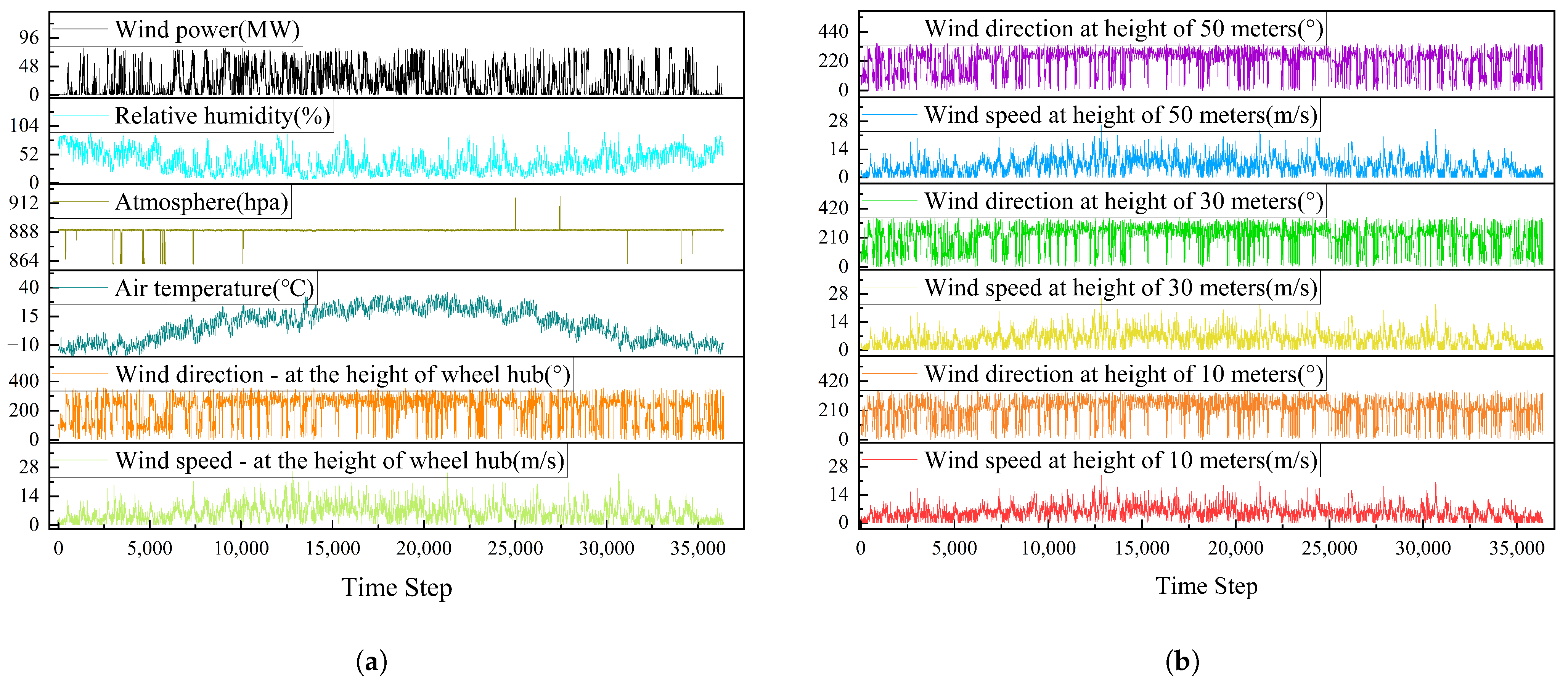
Samples within the dataset are recorded at 15 min intervals. The primary variables include wind speed and wind direction at 10 m, 30 m, 50 m, and hub height, along with environmental features such as air temperature, atmospheric pressure, relative humidity, and the actual power output. Figure 2 illustrates the observational data for Site 1.

To ensure the quality and consistency of the input data, the dataset undergoes comprehensive preprocessing. Missing values are handled and outliers are removed from the raw records. Subsequently, instance normalization is applied to each feature sequence to eliminate the adverse effects of disparate physical units and numerical scales on network training. After preprocessing, the dataset is split in chronological order to prevent information leakage from future observations. Specifically, the original time series is divided into a training set (75%), a validation set (10%), and a testing set (5%). Within each subset, a sliding window mechanism is adopted to construct supervised learning samples, utilizing historical information from the previous consecutive time steps to generate the power prediction.

3.2. Adaptive Signal Decomposition via ISSAVMD

To manage the strong non-stationarity of offshore wind power series, an adaptive signal decomposition method is implemented as the frontend of the forecasting framework. The VMD is employed to non-recursively decompose the complex multivariate wind power time series into a predefined number of band-limited subcomponents, termed intrinsic mode functions (IMFs). This decomposition effectively isolates the underlying low-frequency trend component from the high-frequency stochastic fluctuations and noise, thereby overcoming the limitations of traditional mode decomposition methods such as mode mixing and endpoint effects. The mathematical formulation of variational mode decomposition frames the decomposition as a constrained variational optimization problem, minimizing the sum of the estimated bandwidths of each mode subject to the constraint that the sum of all modes equals the original signal.

The performance of variational mode decomposition is highly sensitive to two key parameters, namely the number of modes K and the penalty factor $\alpha$. An insufficient value for K leads to under-decomposition and the loss of critical high-frequency information, whereas an excessive value introduces spurious modes. The penalty factor $\alpha$ determines the bandwidth of each mode and directly affects the capability of noise separation. To determine the optimal parameter configuration robustly, an improved sparrow search algorithm (ISSA) is introduced. The standard sparrow search algorithm is prone to a loss of population diversity in later iterations, which increases the risk of being trapped in local optima. To enhance global exploration and local exploitation capabilities, ISSA refines the search mechanism through three strategic improvements.

• (1) Logarithmic-Space Initialization

Since the VMD parameters K and $\alpha$ usually span multiple orders of magnitude, logarithmic-space initialization is adopted to ensure uniform population distribution.

For the i-th individual in the population, the parameter vector is defined as:

$${\mathbf{x}}_i=[{\alpha }_i,K_i],i=1,2,\dots ,N.$$

(1)

The penalty factor $\alpha$ is initialized in the logarithmic space to ensure uniform coverage over multiple orders of magnitude:

$${\alpha }_i=\exp \left(\log \left({\alpha }_{\min }\right)+r_i^{\left(1\right)}\left[\log \left({\alpha }_{\max }\right)-\log \left({\alpha }_{\min }\right)\right]\right),r_i^{\left(1\right)}\sim \mathcal{U}(0,1).$$

(2)

The mode number K is initialized in the linear space as:

$$K_i=K_{\min }+r_i^{\left(2\right)}\left(K_{\max }-K_{\min }\right),r_i^{\left(2\right)}\sim \mathcal{U}(0,1),$$

(3)

where $\exp (·)$ denotes the natural exponential function; $r_i\sim \mathcal{U}(0,1)$ denotes a random variable uniformly distributed over the interval $(0,1)$; ${\alpha }_{\min }$ and ${\alpha }_{\max }$ denote the lower and upper bounds of the penalty factor, respectively, and $K_{\min }$ and $K_{\max }$ are the bounds of the mode number; the exponential mapping transforms uniformly sampled values from the logarithmic space back to the original parameter space.

• (2) Lévy Flight Mechanism

To mitigate premature convergence in the later optimization stages, a Lévy flight perturbation mechanism is introduced [37]. The Lévy step is defined as:

$$\mathrm{Levy}\left(\lambda \right)={\displaystyle \frac{\mu }{{\left|\nu \right|}^{1/\lambda }}}$$

(4)

$$\sigma ={\left({\displaystyle \frac{\Gamma (1+\lambda )\sin (\pi \lambda /2)}{\Gamma \left(\frac{1+\lambda }{2}\right)\lambda 2^{(\lambda -1)/2}}}\right)}^{1/\lambda }$$

(5)

where $\lambda \in (1,3)$ is the Lévy exponent controlling the jump intensity, $\mu$ and $\nu$ are random variables following normal distributions, and $\Gamma (·)$ denotes the Gamma function.

For exploitation-oriented individuals, Lévy flight-based updates are applied:

$$X_i^{t+1}=X_i^t+\mathrm{Levy}\left(\lambda \right)\left(X_i^t-X_{\mathrm{best}}\right).$$

(6)

• (3) Hierarchical Sine–Cosine Search Strategy

To enhance search direction diversity, a sine–cosine search strategy is incorporated with hierarchical population updating [38]. For exploration-oriented individuals, the position update is given by:

$$X_i^{t+1}=X_i^t+r_1\left\{\begin{array}{c}\sin \left(r_2\right)\left|r_3{X}_{\mathrm{best}}-X_i^t\right|,\hfill \\ \cos \left(r_2\right)\left|r_3{X}_{\mathrm{best}}-X_i^t\right|,\hfill \end{array}\right.$$

(7)

where $r_1$ controls the convergence speed, $r_2\in [0,2\pi ]$, $r_3\in [0,2]$, and $X_{\mathrm{best}}$ denotes the global best solution.

To prevent data leakage and maintain strict causality, the parameter optimization process of ISSA-VMD is strictly restricted to the training and validation sets. The static parameters K and $\alpha$ derived from the training sequence are subsequently applied as parallel band-pass filters to decompose the testing set.

3.3. Theoretical Analysis of ISSA

To rigorously justify the advantages of the proposed improvements over the standard SSA, this subsection provides a theoretical analysis from two complementary perspectives: population diversity preservation and escape capability from local optima.

• Preliminaries: Tail Properties of Lévy Distributions

The Lévy flight step generated by the Mantegna algorithm [39] follows a heavy-tailed distribution. Specifically, for a step $L\sim \mathrm{Levy}\left(\lambda \right)$, the tailprobability satisfies

$$P\left(\right|L|>s)\sim s^{-\lambda },\lambda \in (1,3),$$

(8)

for sufficiently large $s>0$. In contrast, a Gaussian-type perturbation $G\sim \mathcal{N}(0,{\sigma }^2)$ exhibits an exponentially decaying tail:

$$P\left(\right|G|>s)\sim \exp \left(-{\displaystyle \frac{s^2}{2{\sigma }^2}}\right).$$

(9)

This contrast between power-law and exponential tail decay is the mathematical foundation of the advantages established below [40,41].

Proposition 1

(Lower Bound on Population Diversity). Define the population diversity at iteration t as

$$D\left(t\right)={\displaystyle \frac{1}{N}}{\displaystyle \sum _{i=1}^N}{∥X_i^t-{\overline{X}}^t∥}_2,{\overline{X}}^t={\displaystyle \frac{1}{N}}{\displaystyle \sum _{i=1}^N}{X}_i^t.$$

(10)

Let $D_{\mathrm{SSA}}\left(t\right)$ and $D_{\mathrm{ISSA}}\left(t\right)$ denote the population diversity of the standard SSA and the proposed ISSA, respectively. Under identical initial conditions, there exist positive constants $c_1,c_2$ such that

$$\begin{array}{cc}\hfill \mathbb{E}\left[D_{\mathrm{SSA}}\left(t\right)\right]& \le c_1\exp (-\beta t),\hfill \end{array}$$

(11)

$$\begin{array}{cc}\hfill \mathbb{E}\left[D_{\mathrm{ISSA}}\left(t\right)\right]& \ge c_2·t^{-1/\lambda },\hfill \end{array}$$

(12)

where $\beta >0$ is determined by the convergence factor of SSA, $\mathbb{E}[·]$ represents the mathematical expectation, and λ is the Lévy index in (8).

Sketch of proof. (i) For the standard SSA, the position update rule asymptotically reduces to a contraction mapping toward the current best solution $X_{\mathrm{best}}$:

$$X_i^{t+1}=X_i^t+{\alpha }_t(X_{\mathrm{best}}-X_i^t)+{\xi }_t,$$

where ${\alpha }_t\in (0,1)$ is the effective step size and ${\xi }_t$ is a bounded-variance perturbation. Taking norms and expectations yields the recursion

$$\mathbb{E}\left[\parallel X_i^{t+1}-{\overline{X}}^{t+1}{\parallel }_2\right]\le (1-{\alpha }_t)\mathbb{E}\left[\parallel X_i^t-{\overline{X}}^t{\parallel }_2\right],$$

which iterates to the exponential bound in (11).

(ii) In ISSA, exploitation-oriented individuals follow

$$X_i^{t+1}=X_i^t+\mathrm{Levy}\left(\lambda \right)\odot (X_i^t-X_{\mathrm{best}}),$$

in which the Lévy step has infinite variance. By (8), for any threshold s,

$$P\left(\parallel X_i^{t+1}-{\overline{X}}^{t+1}{\parallel }_2>s\right)\ge C{s}^{-\lambda }.$$

Generalised moment inequalities then imply that the expected diversity cannot decay faster than the power-law rate (12). □

Remark 1.

Proposition 1 establishes a strict tail-rate contrast: the diversity of the standard SSA collapses exponentially fast toward $X_{\mathrm{best}}$, so its later iterations effectively degenerate into local search. In contrast, ISSA preserves non-trivial diversity at a power-law rate, which is essential for navigating the strongly multi-modal landscape of the VMD parameter space.

Proposition 2

(Lower Bound on Escape Probability). Suppose the population is trapped in an ϵ-neighbourhood $B(X^{\star },ϵ)=\{X:\parallel X-X^{\star }{\parallel }_2\le ϵ\}$ of a local optimum $X^{\star }$. The single-step escape probability satisfies

$$\begin{array}{cc}\hfill P_{\mathrm{escape}}^{\mathrm{SSA}}& \le c_3\exp \left(-{\displaystyle \frac{{ϵ}^2}{2{\sigma }^2}}\right),\hfill \end{array}$$

(13)

$$\begin{array}{cc}\hfill P_{\mathrm{escape}}^{\mathrm{ISSA}}& \ge c_4{ϵ}^{-\lambda },\hfill \end{array}$$

(14)

where $c_3,c_4>0$ are constants independent of the initial position.

Sketch of proof. 

The escape probability is given by $P\left(\parallel X^{t+1}-X^{\star }{\parallel }_2>ϵ\right)$. For the standard SSA, the perturbation is dominated by bounded random numbers and Gaussian-type noise, whose tails are governed by (9); this yields (13). For ISSA, the Lévy step in the exploitation update directly contributes a heavy-tailed term to $\parallel X^{t+1}-X^t{\parallel }_2$, and (8) gives

$$P\left(\parallel \mathrm{Levy}\left(\lambda \right)\odot (X_i^t-X_{\mathrm{best}}){\parallel }_2>ϵ\right)\ge C{ϵ}^{-\lambda },$$

which yields (14). □

Remark 2.

Proposition 2 reveals an order-of-magnitude difference: when ϵ is large (i.e., the local optimum is deep), the escape probability of standard SSA decays as $\exp (-{ϵ}^2)$ and is practically zero, whereas ISSA decays only as ${ϵ}^{-\lambda }$ and retains a non-negligible escape rate. This is particularly important when the VMD parameters $(\alpha ,K)$ span multiple orders of magnitude.

Remark 3

(Directional Coverage of the Sine-Cosine Strategy). Beyond the step-size scale, ISSA also extends the geometric coverage of search directions through the sine-cosine modulation. The update direction in Equation (7) takes the form

$$v(r_1,r_2)=r_1\sin \left(r_2\right)(X_{\mathrm{best}}-X_i^t),r_2\in [0,2\pi ].$$

Since $\sin \left(r_2\right)$ takes values across the full range $[-1,1]$, the search direction includes both toward and away from the current best, in contrast with the standard SSA, which contracts only along the direction $X_{\mathrm{best}}-X_i^t$. Combined with the heavy-tailed step distribution in Proposition 1, ISSA achieves improvements over standard SSA in both step-size scale and search direction.

• Synthesis

Together, the three results above demonstrate the theoretical superiority of ISSA, summarised in

Table 2. Theoretical comparison between standard SSA and ISSA.

Property	Standard SSA	ISSA
Diversity decay rate	$\exp (-\beta t)$	$t^{-1/\lambda }$
Escape probability from $B(X^{\star },ϵ)$	$\exp (-{ϵ}^2/2{\sigma }^2)$	${ϵ}^{-\lambda }$
Search direction	Unidirectional (toward $X_{\mathrm{best}}$)	Omnidirectional

.

These properties are particularly desirable in the multi-modal, multi-scale VMD parameter optimisation scenario considered in this paper.

3.4. Collaborative Temporal-Channel Modeling via TCN-SOFTS

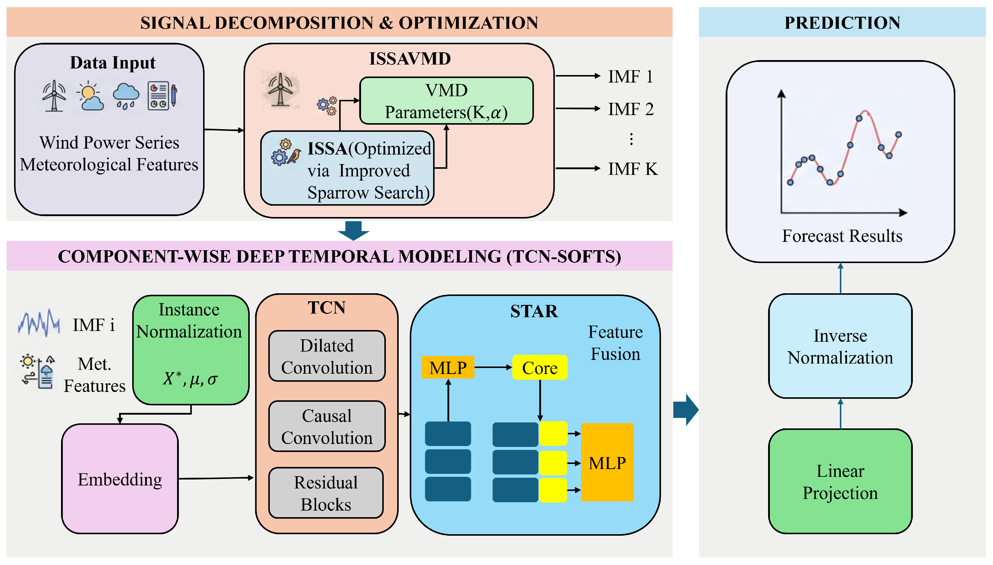
Following the adaptive signal decomposition, the extracted IMFs and meteorological features are mapped into a high-dimensional latent space through a linear embedding layer after instance normalization. To capture the complex multiscale temporal dynamics and multivariate dependencies within the expanded channel space, the framework integrates a TCN with the SOFTS architecture. The TCN serves as the core backend for local temporal modeling, processing the embedded representations through stacked dilated causal convolutional layers. By adjusting the dilation factor exponentially, the receptive field of the network expands to cover extensive historical sequences without incurring excessive parameter overhead. The incorporation of causal constraints ensures that the output at any given time step depends solely on current and historical inputs, thereby strictly preserving temporal causality. Furthermore, residual connections are integrated across the stacked layers to alleviate the problem of gradient vanishing, supporting the stable training of deep network structures.

To counterbalance the substantial computational overhead introduced by the increased dimensionality of the feature space after signal decomposition, the global channel dependencies are modeled utilizing the STAR module of the SOFTS architecture. Traditional attention mechanisms exhibit quadratic or higher computational complexity regarding the number of channels, making them computationally unviable for high-dimensional multivariate time series. In contrast, the STAR module adopts a centralized aggregation–redistribution strategy to achieve global channel interaction with strictly linear complexity. The embedded representations of all channels are first projected into a lower-dimensional space, and stochastic pooling is applied across the channels to generate a unified core representation. This core representation encapsulates the global statistical regularities and inter-variable correlations of the entire system. Subsequently, the core representation is replicated and concatenated with each individual channel feature, passing through a multilayer perceptron to produce channel-aware representations that efficiently fuse global context while preserving channel-specific information. Finally, the channel features are fused, projected back to the power output space via a linear layer, and inverse-normalized. The individual forecasting results of all IMFs are aggregated to produce the final offshore wind power prediction, resolving the inherent conflict between signal fidelity and computational efficiency.

The overall forecasting procedure and model architecture of the proposed ISSAVMD-TCN-SOFTS are illustrated in Figure 3.

3.5. Model Hyperparameters and Experimental Platform

The model hyperparameter configuration includes the training batch size, model dimensionality, the number of encoder blocks, and the dimensionality of the fully connected network. The detailed parameter settings are listed in

Table 3. Configuration of model hyperparameters and experimental platform.

Category	Parameter	Value	Category	Parameter	Value
Input	Window length	96	Model	Dropout	0.2
Input	Input dimension	12	Training	Batch size	128
Model	d_model	64	Training	Learning rate	0.001
Model	Number of heads	8	Training	Epochs	500
Model	Encoder layers	12	stop_ratio	stop_ratio	0.2
Model	Decoder layers	12	Output	Output dimension	1

. All experiments are conducted using Python 3.8 on a workstation equipped with an NVIDIA RTX 4090 GPU and an Intel(R) i9-14900KF CPU operating at 3.2 GHz.

4. Simulation Results

4.1. VMD Result

Table 4. Optimal VMD parameters (K and $\alpha$) obtained via ISSA for different sites.

Site	K	$\mathit{\alpha }$
1	2	5042.36
2	2	4312.85
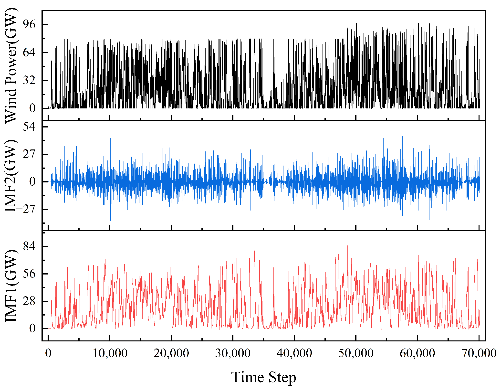
3	3	3874.69

details the optimal modal decomposition parameters for each site obtained through the ISSA method. To prevent data leakage, the parameter search for VMD is strictly confined to the training and validation sets. The static parameters K and $\alpha$ extracted from the training set configure parallel band-pass filters, which subsequently decompose the test set into Intrinsic Mode Functions (IMFs) to guarantee a causal decomposition procedure. Figure 4 illustrates the decomposed power sequence for the training set of Site 1.

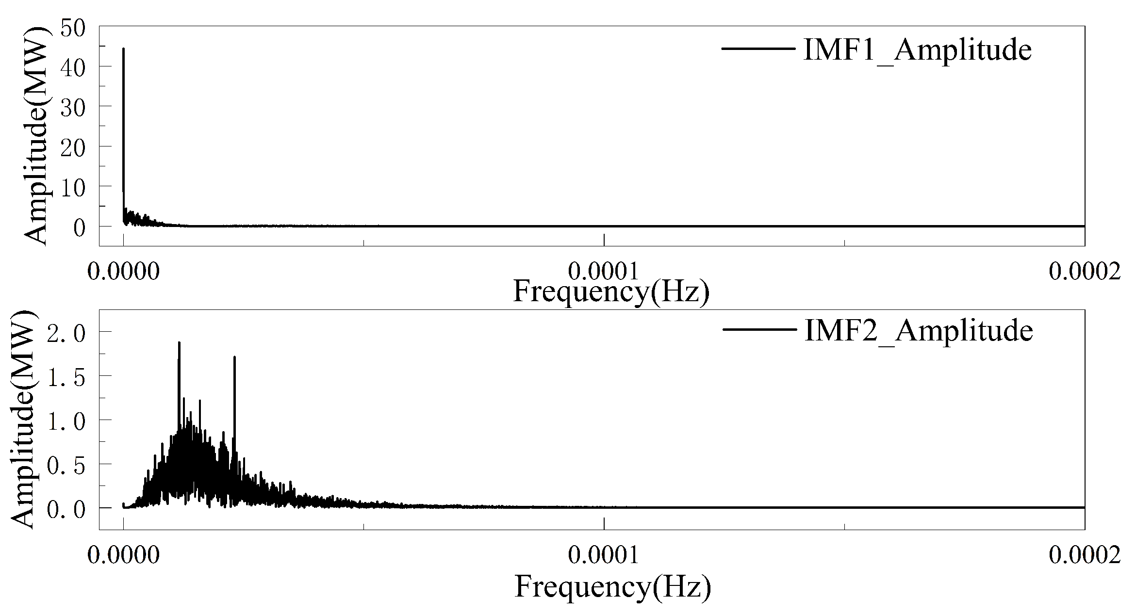
As demonstrated in Figure 5, the energy of IMF1 is highly concentrated near zero frequency with an exceptionally narrow bandwidth, confirming the role of the component as the dominant trend. Furthermore, the spectrum of IMF2 is distributed across a broader frequency band containing multiple local peaks, identifying the function as the dynamic fluctuation component. Consequently, this dual-component decomposition strictly isolates the underlying trend from the high-frequency dynamic noise. As illustrated in Figure 4, the original offshore wind power time series is decomposed into two IMFs exhibiting distinct frequency characteristics. Specifically, IMF1 delineates the low-frequency trend component of the wind power, reflecting the fundamental variation and long-term evolution of the sequence. Conversely, IMF2 corresponds to the high-frequency fluctuation component, capturing the stochastic disturbances and complex non-stationarity inherent in the data. To further validate the effectiveness of the decomposition, a frequency spectrum analysis is conducted.

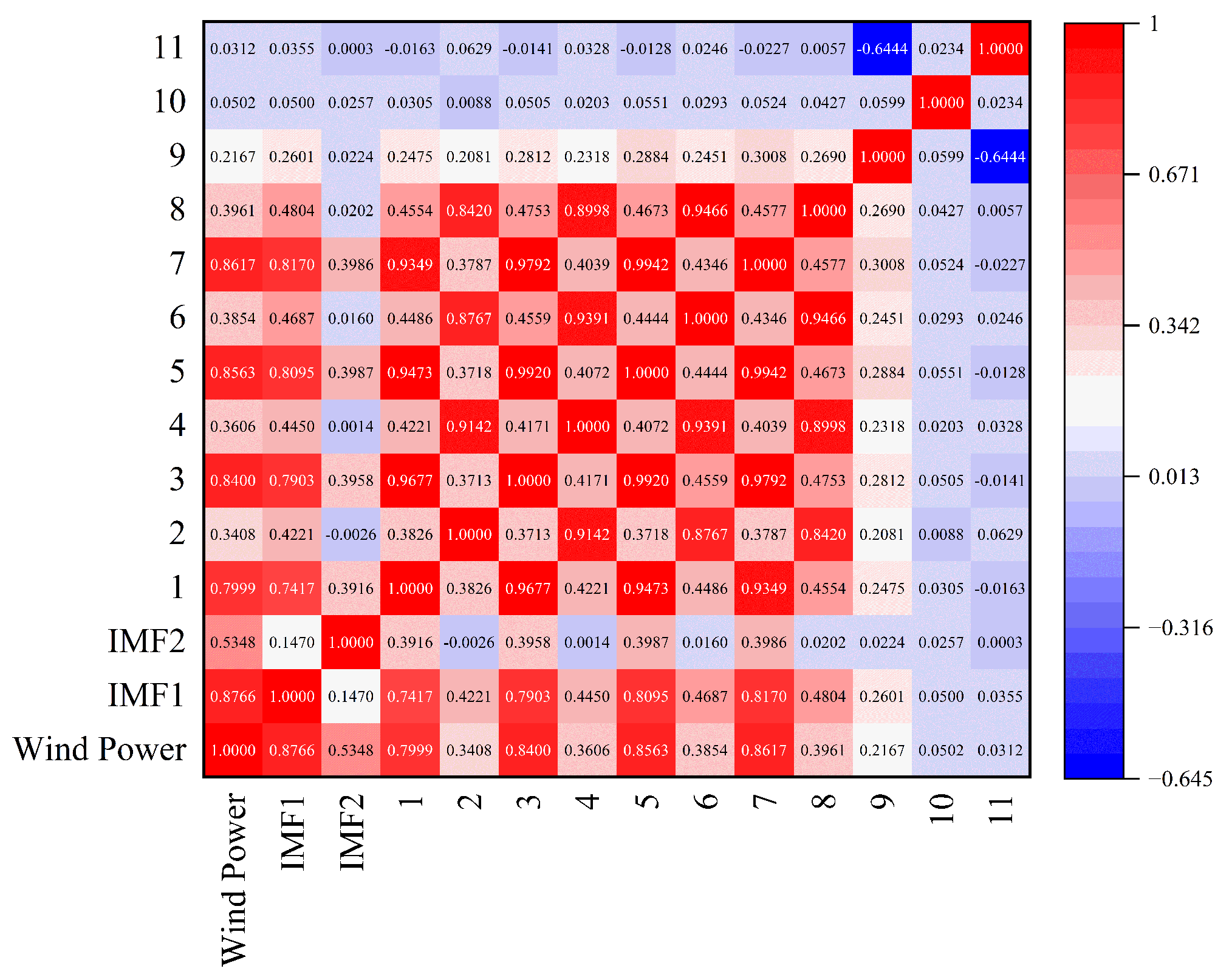
Figure 6 presents the Pearson correlation matrix among the decomposed components, the target power, and the input meteorological features. IMF1 correlates strongly with the target power ($r=0.8766$), confirming its role as the dominant trend component in the wind power series. It is highly sensitive to wind speeds at various heights, particularly at the hub height (variable 7), with a correlation of 0.8170. The higher-frequency fluctuation component, IMF2, exhibits a moderate correlation with the target ($r=0.5348$) and generally weaker links to meteorological features. Its correlation with relative humidity (variable 11), for example, approaches zero. These distinct physical dependencies confirm that the decomposition effectively isolates predictive subcomponents for subsequent modeling.

4.2. Comparison of Model Performance

The proposed framework is evaluated against several baseline models: DLinear (2023), CrossLinear (2025), iTransformer (2024), PatchTST (2023), Time TK (2026), and GTR (2026). Given a 15 min temporal resolution, the forecasting horizons are set to 12, 24, 48, and 96 steps (corresponding to 3, 6, 12, and 24 h). To ensure statistical stability and reliability, each experiment is independently repeated ten times to mitigate the influence of random weight initialization. The reported evaluation metrics represent the arithmetic mean of these ten trials.

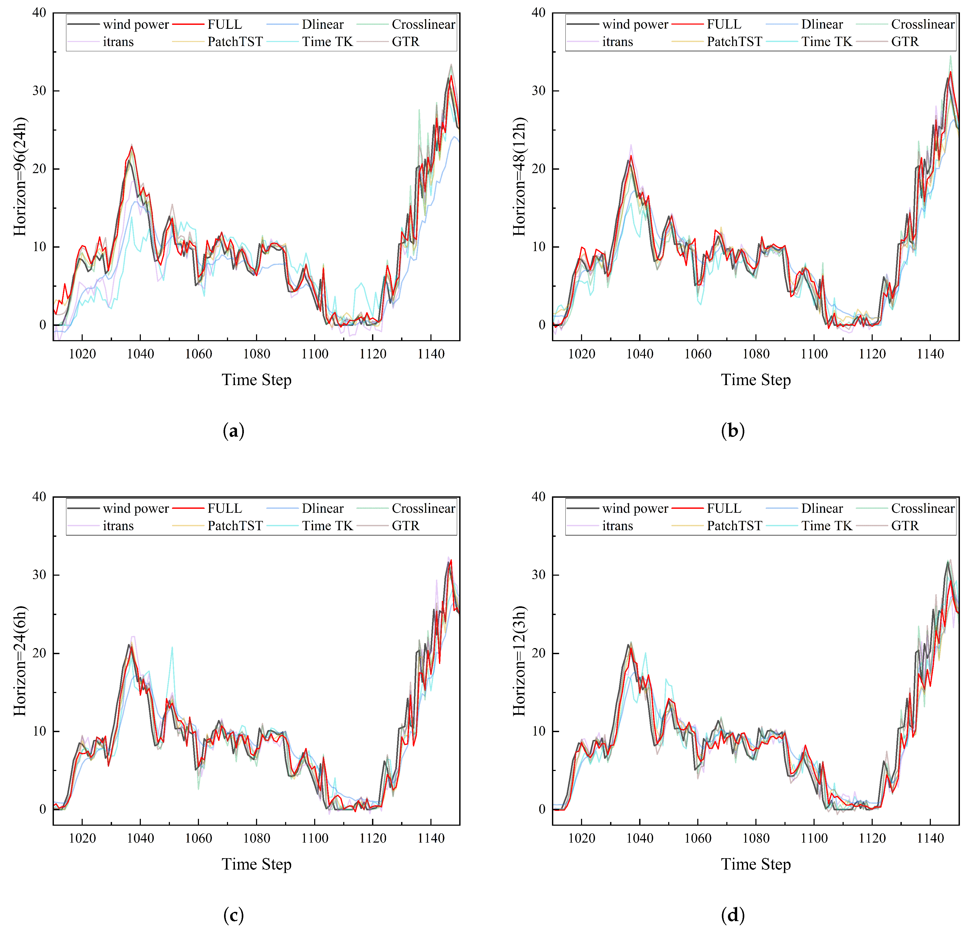
As detailed in

Table 5. Performance comparison of forecasting models across different sites and horizons.

Site	Horizon	FULL (Ours)		Dlinear		Crosslinear		iTrans		PatchTST		Time TK		GTR
		MAE	RMSE	MAE	RMSE	MAE	RMSE	MAE	RMSE	MAE	RMSE	MAE	RMSE	MAE	RMSE
1	96	0.4601	1.1660	0.6862	1.3611	0.4676	1.1842	0.5193	1.2514	0.4134	1.0871	0.4192	1.2152	0.4645	1.2630
	48	0.4008	1.1297	0.6880	1.3881	0.4465	1.0288	0.5188	1.2923	0.5298	1.3319	0.3944	1.2538	0.4570	1.1761
	24	0.3937	0.9828	0.8365	1.4191	0.3895	1.0081	0.4682	0.8365	0.4342	1.1837	0.3919	1.2417	0.3793	1.0396
	12	0.3415	0.8269	0.9566	0.4905	0.3861	1.0669	0.4588	1.1447	0.4295	1.2211	0.4427	1.2691	0.3778	1.0220
2	96	2.0103	3.1470	2.2306	3.4406	1.4633	2.6116	1.6355	2.8870	1.6818	2.8038	1.6294	8.7125	1.4221	6.6547
	48	1.3446	2.4297	2.1729	3.3502	1.6748	3.1243	1.6140	2.9546	1.7010	2.8694	1.6317	8.4943	1.3444	6.2915
	24	1.2065	1.9238	2.2669	3.4379	1.5054	2.7542	1.5788	2.8310	1.6407	2.9183	1.5107	7.5999	1.3105	6.1507
	12	1.1718	1.8457	2.4228	3.5050	1.4996	2.7077	1.5703	2.8646	1.5584	2.8904	1.5990	8.6905	1.3462	6.5165
3	96	2.3355	3.3042	4.4787	5.6388	1.6095	2.4430	2.2364	2.8824	1.8886	2.5135	1.8110	6.6286	1.8214	5.6604
	48	1.3702	2.5469	2.8904	3.8674	1.4590	2.1195	1.7534	2.5126	1.9123	2.5123	1.5386	4.8281	1.3780	3.9440
	24	1.3172	1.8667	2.8134	3.8588	1.4182	2.0654	1.6756	2.4050	1.5722	2.2596	1.6433	5.8316	1.3805	4.0797
	12	1.1401	1.5926	2.5507	3.5354	1.3698	2.0237	1.7343	2.5422	1.6996	2.5080	1.6882	6.0907	1.3485	3.8745

Note: Bold entries represent the optimal performance metrics for each evaluation condition.

, the proposed model consistently achieves lower MAE and RMSE values compared to all baseline models across all horizons. Specifically, at Site 1 for the 96-step horizon, the proposed model reduces the MAE by 14.3% and the RMSE by 30.0% relative to the DLinear model. This improvement is more pronounced at Site 3, where environmental volatility is higher; here, the proposed architecture achieves an error reduction of approximately 41.4% in MAE and 47.8% in RMSE compared to the DLinear baseline. Qualitative evaluation via the prediction trajectories in Figure 7 confirms that the proposed model tightly traces the actual wind power sequence across all horizons, maintaining high fidelity at local extrema during sudden power ramps.

4.3. Ablation Study

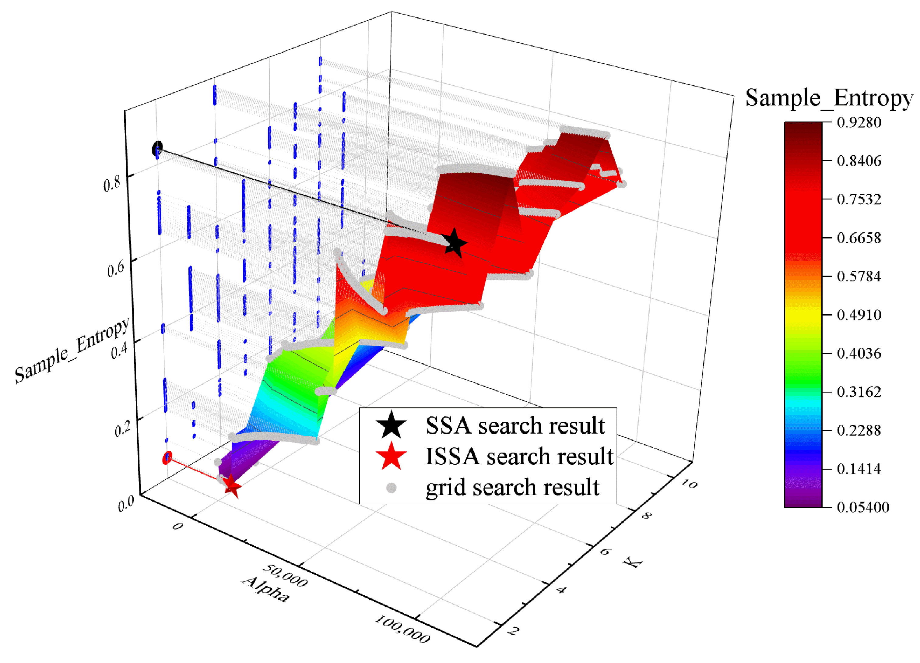
To isolate the quantitative contribution of each distinct module, systematic ablation studies are conducted for both the signal decomposition frontend and the deep learning backend. The performance of the ISSAVMD frontend is compared with alternative decomposition techniques, including EMD, ICEEMDAN, and standard SSAVMD, as shown in

Table 6. Comparison of different decomposition models with bolded optimal values.

Model	ISSAVMD		SSAVMD		Grid-SearchVMD		ICEEMDAN		EMD
Metric	MAE	RMSE	MAE	RMSE	MAE	RMSE	MAE	RMSE	MAE	RMSE
48	0.6059	1.2605	0.5827	1.2642	0.4860	1.2741	0.7146	1.9077	1.7231	1.6538
24	0.3937	0.9828	0.5116	1.3347	0.4709	1.1240	0.5167	1.0855	0.5004	1.2179
12	0.3415	0.8269	0.4594	1.2769	0.4407	1.1345	0.3825	0.8588	0.3976	1.9148

Note: Bold entries represent the optimal performance metrics for each evaluation condition.

. The optimization process is further illustrated by the hyperparameter search trajectories in Figure 8.

To systematically investigate the contribution of the temporal modeling and the channel modeling components within the proposed predictive architecture, an extensive ablation study is conducted. Specifically, the complete model, denoted as FULL, is compared against five variants: CNN-SOFTS (which replaces the TCN with a CNN), SOFTS, TCN-MLP (which substitutes the SOFTS module with a MLP), TCN-LSTM (which substitutes the SOFTS module with a LSTM), and MLP. To ensure a rigorous and fair comparison of the backend architectures, the input data for all evaluated models are preprocessed utilizing the identical ISSAVMD frontend. The comparative results across multiple forecasting horizons are detailed in

Table 7. Ablation study results.

Model	FULL		CNN-SOFTS		SOFTS		TCN-MLP		TCN-LSTM		MLP
Metric	MAE	RMSE	MAE	RMSE	MAE	RMSE	MAE	RMSE	MAE	RMSE	MAE	RMSE
48	0.6059	1.2605	0.7030	1.4613	0.6370	1.4082	0.7473	1.3196	0.6714	1.0465	0.8732	1.4093
24	0.3937	0.9828	0.4467	1.2336	0.5288	1.3089	0.6322	1.0844	0.5464	1.1310	0.9106	1.3531
12	0.3415	0.8269	0.4488	1.2512	0.4700	1.2698	0.6345	1.0740	0.5478	1.0275	1.3596	1.5735

Note: Bold entries represent the optimal performance metrics for each evaluation condition.

.

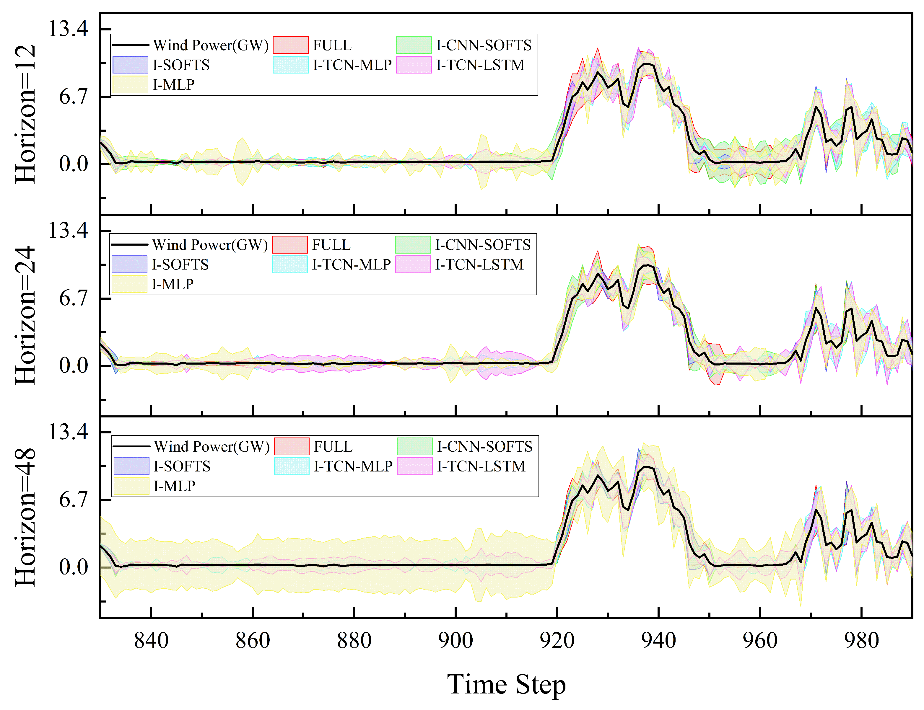
The quantitative contributions of the individual architectural components are further substantiated by the error reductions detailed in

Table 8. Contribution of TCN and ISSAVMD.

Horizon	Metric	TCN Contribution (%)	ISSAVMD Contribution (%)
48	MAE	21.0	−20.5
	RMSE	3.3	7.4
24	MAE	15.5	11.9
	RMSE	5.8	20.3
12	MAE	4.5	23.9
	RMSE	1.5	33.9

, which emphasize the critical role of the TCN in minimizing the MAE. Furthermore, the visualizations of the prediction errors provided in Figure 9 reinforce these statistical conclusions. Specifically, the predictive trajectory of the FULL model tracks the ground truth with superior fidelity, effectively suppressing error propagation and preserving predictive stability during periods of severe meteorological volatility. In contrast, the baseline variants demonstrate pronounced amplitude deviations and temporal phase shifts.

4.4. Interpretability Analysis Based on SHAP

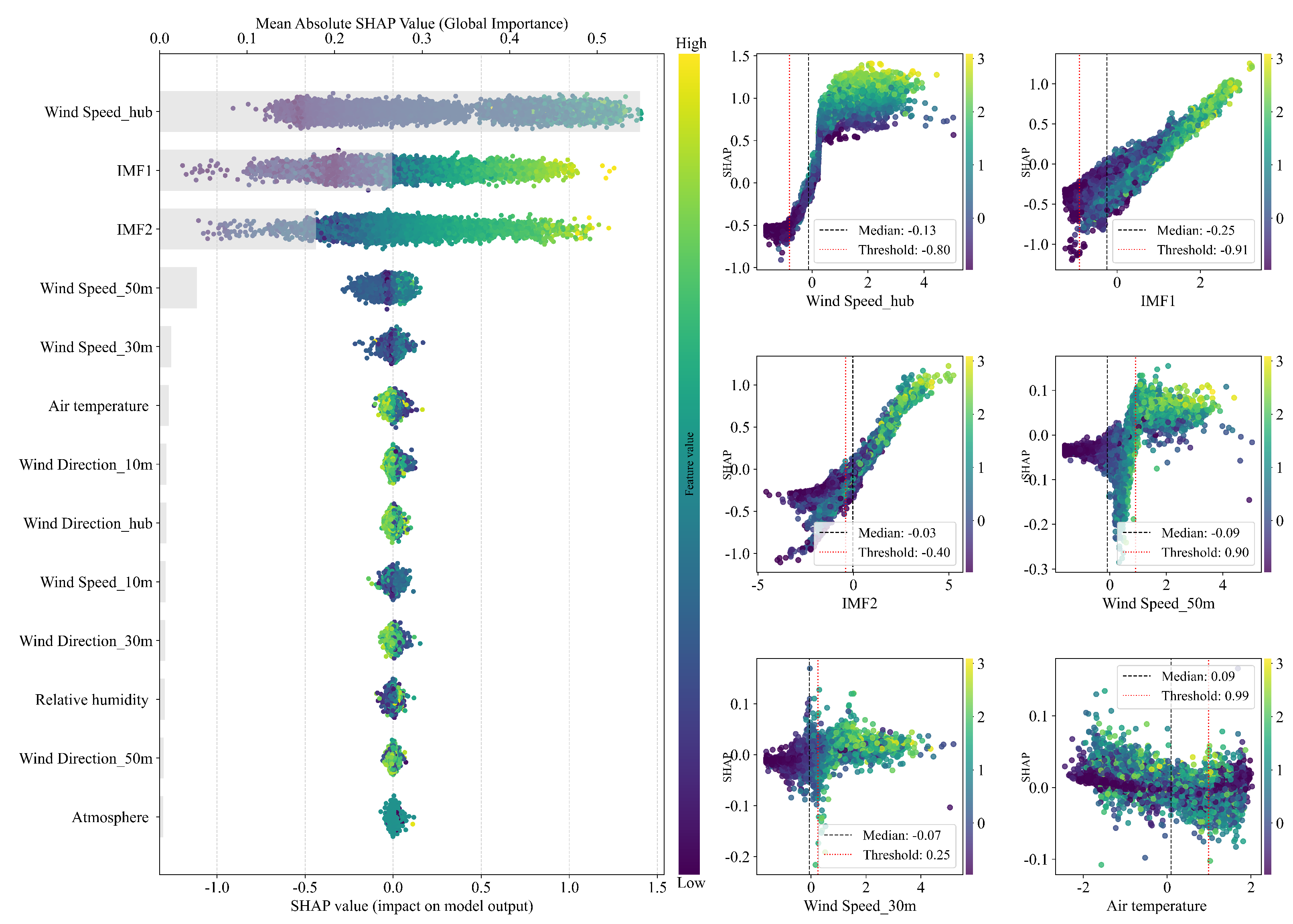
To further elucidate the decision-making mechanism of the proposed framework and quantify the contribution of various meteorological features to wind power prediction, this study employs the SHapley Additive exPlanations (SHAP) method. Figure 10 illustrates the summary plot of mean absolute SHAP values for the primary input variables and the corresponding feature dependence plots. Analysis of the global importance ranking reveals that wind speed at hub height is the most critical determinant, exhibiting the highest mean absolute SHAP value. The color distribution of the scatter points in the summary plot indicates a strictly positive correlation: high feature values, represented by yellow and green points, significantly drive positive model outputs, whereas low values, depicted in dark purple, pull the predictions downward. Furthermore, the Intrinsic Mode Functions, specifically IMF1 and IMF2, follow the primary wind speed in global importance. This high ranking validates the theoretical premise of the proposed framework: the extraction of intrinsic frequency components via adaptive signal decomposition successfully isolates highly predictive features from the original non-stationary signals, thereby fundamentally enhancing the learning efficiency of the network.

4.5. Computational Complexity Metrics

The computational feasibility of the proposed framework is evaluated on a hardware platform equipped with an NVIDIA RTX 4090 GPU and an Intel i9-14900KF CPU. The resource utilization of the model is quantified across three metrics: parameter size, inference latency per sample, and training time per epoch. These empirical complexity metrics are consolidated in

Table 9. Comparison of parameter size, inference latency, and training time among different models.

Model	Parameter Size (M)	Inference Latency (ms/Sample)	Training Time (s/Epoch)
FULL	0.2149	1.0797	2.1567
Dlinear	0.0872	0.0084	1.1276
Crosslinear	0.0619	0.025	1.1539
itrans	0.2568	0.0361	2.9382
PatchTST	0.2516	0.0026	2.8749
Time TK	0.1017	0.0094	2.2429
GTR	0.0241	0.0032	1.9484

.

5. Discussion

The consistent error reductions achieved by the proposed framework across multiple forecasting horizons underscore the limitations of simpler linear models and conventional recurrent or Transformer-based architectures. Linear models, such as DLinear and CrossLinear, exhibit competitive mean absolute errors in short-term scenarios but suffer from substantial prediction volatility over extended horizons. This vulnerability stems from the inherent inability of linear layers to capture the complex, non-stationary dynamics governing marine environments. Although Transformer-based architectures utilize global attention mechanisms to model long-range sequences, the models frequently suffer from semantic misalignment when processing continuous numerical time series, leading to severe overfitting on noisy high-frequency wind power data. The structural integration of the TCN backend resolves these limitations by modeling multi-scale local temporal dependencies through dilated causal convolutions while enforcing strict temporal causality. Concurrently, the core representation mechanism within the SOFTS architecture effectively captures global channel dependencies with linear computational complexity, mitigating the representation constraints of standard multilayer perceptrons in high-dimensional state spaces. This synergistic integration allows the proposed model to maintain robust overall stability as the forecasting horizon extends, closely tracking the true dynamic trajectory during rapid power ramps and sudden drops without severe phase lag or amplitude distortion.

Beyond empirical predictive performance, the interpretable quantification utilizing SHAP values provides a transparent and physically consistent justification for the model outputs. The quantified trajectory for the wind speed at hub height demonstrates a steep gradient near a median threshold before reaching a saturation plateau. This non-linear behavior closely mirrors the physical power curve of a standard wind turbine, where power generation increases monotonically with wind velocity until reaching the maximum limit at the rated wind speed. Secondary environmental variables, such as air temperature, exhibit threshold-dependent contributions, reflecting complex physical interactions with air density that indirectly modulate the efficiency of energy conversion.

The empirical superiority of the optimization strategy is intrinsically governed by the theoretical attributes analyzed in Section 3.3. Specifically, the established lower bound on the escape probability of the ISSA method enables the algorithm to navigate the highly non-convex parameter landscape effectively, thereby preventing premature convergence to suboptimal states. In physical deployment, this enhanced global search capability manifests as the successful identification of VMD parameter configurations that yield a significantly higher sample entropy. By achieving this optimal parameterization, the framework fundamentally mitigates the detrimental effects of mode mixing, thereby ensuring that the decomposed IMFs maintain an exceptionally high degree of feature purity. This high fidelity in feature representation directly enhances the learning efficiency of the downstream network; when encountering extreme power ramp events characterized by high-frequency volatility, the predictive backend exhibits a pronounced reduction in phase delay alongside a significant decrease in the RMSE, thereby establishing a direct causal link between theoretical escape guarantees and practical forecasting robustness.

Regarding architectural deployment, the integration of the adaptive signal decomposition frontend, the TCN, and the SOFTS introduces a trade-off between structural complexity and computational efficiency. Although these interconnected components increase the parameter size and inference latency relative to ultra-lightweight linear baselines, the absolute computational overhead of the complete framework remains exceptionally low. The documented inference latency of 1.0797 ms per sample is several orders of magnitude below the temporal resolution of 15 min required for real-time ultra-short-term and short-term power system scheduling. This substantial operational margin demonstrates that the framework completely satisfies the real-time constraints of modern wind farm dispatch systems directly on local hardware.

6. Research Review

A retrospective evaluation of the research trajectory microfilm established in this study demonstrates a systematic advancement in the domain of offshore wind power forecasting. The investigation successfully addresses the critical challenges of extreme non-stationarity and complex multivariate coupling inherent in marine meteorological environments. By establishing a closed-loop framework, this research validates the theoretical synergy between adaptive signal processing and lightweight deep temporal-channel modeling.

The empirical evaluations of the proposed framework provide clear answers to the research questions formulated in the introduction.

• In response to RQ1

The theoretical and empirical analyses of the improved sparrow search algorithm demonstrate that the integration of Lévy flight and sine–cosine modulation successfully navigates the non-convex parameter space of variational mode decomposition. As illustrated by the search trajectories and the ablation studies of the decomposition models, this optimization strategy prevents premature convergence and identifies parameter configurations that yield high sample entropy. Furthermore, this parameter optimization process is strictly restricted to the training and validation sets to prevent data leakage and ensure causality.

• In response to RQ2

The integration of the temporal convolutional network and the SOFTS architecture provides a robust solution for deep temporal modeling. The ablation study regarding the forecasting architecture confirms that dilated causal convolutions effectively extract local temporal dependencies, while the core representation mechanism of the SOFTS module captures global channel dependencies with linear computational complexity. This structural synergy mitigates the representation constraints of standard architectures without introducing disastrous computational overhead.

• In response to RQ3

The comprehensive comparison across multiple forecasting horizons and diverse offshore sites demonstrates that the ISSAVMD-TCN-SOFTS framework consistently outperforms mainstream linear, recurrent, and Transformer-based models. The proposed framework significantly reduces the mean absolute error and the root mean square error, maintaining high predictive fidelity and operational stability during extreme meteorological fluctuations.

7. Limitations of Research

Despite the superior accuracy and robust stability demonstrated by the complete model, a critical review of the current framework identifies specific boundaries and open avenues for further enhancement. Although the inference latency fully satisfies the real-time constraints of modern wind farm dispatch systems, the initial frontend signal decomposition phase introduces a noticeable computational requirement during the offline training process. This characteristic suggests the necessity of developing accelerated, parallelized decomposition algorithms to minimize the total computational overhead in large-scale deployments. Furthermore, the predictive architecture currently operates primarily on data-driven meteorological and operational inputs, omitting physical hardware-level constraints. Incorporating downstream engineering parameters, such as the switching losses of power electronic equipment, inverter efficiency curves, and turbine degradation profiles, would refine the practical utility of the forecasting outputs. Consequently, this retrospective review establishes a clear trajectory for future investigations, emphasizing the integration of hardware-level loss factors and the acceleration of signal processing pipelines to further bridge the gap between theoretical models and real-world industrial deployment.

8. Conclusions

This study develops a hybrid forecasting framework, termed ISSAVMD-TCN-SOFTS, to enhance the accuracy and stability of offshore wind power prediction. The developed architecture effectively demonstrates the validity of the research by systematically addressing the proposed research questions.

The framework successfully mitigates the severe non-stationarity of wind power sequences by utilizing an improved sparrow search algorithm to adaptively optimize the parameters of variational mode decomposition. By combining the multiscale local feature extraction capability of temporal convolutional networks with the global channel dependency modeling of the STAR module, the framework achieves a synergistic representation of complex meteorological interactions with strictly linear computational complexity. Rigorous empirical evaluations conducted on multi-site operational datasets demonstrate that the proposed framework consistently outperforms mainstream baselines, yielding substantial reductions in both the mean absolute error and the root mean square error. Ultimately, by successfully resolving the inherent conflict between signal fidelity and computational complexity, this work provides a highly effective, robust, and economically viable solution for modern offshore wind power integration and power system scheduling.

References

1. Global Wind Energy Council. Global Wind Report 2024; Technical Report; Global Wind Energy Council: Brussels, Belgium, 2024. [Google Scholar]
2. Wang, T.; Du, G.; He, J. China Wind Power 2023: Installation Capacity Statistics; Technical Report; Chinese Wind Energy Association: Beijing, China, 2024. [Google Scholar]
3. Porté-Agel, F.; Bastankhah, M.; Shamsoddin, S. Wind-Turbine and Wind-Farm Flows: A Review. Bound.-Layer Meteorol. 2020, 174, 1–59. [Google Scholar]
4. Luo, B.X.; Zuo, P.; Zhu, L.J.; Hua, W. A Wind Power Density Forecasting Model Based on RF-DBO-VMD Feature Selection and BiGRU Optimized by the Attention Mechanism. Atmosphere 2025, 16, 266. [Google Scholar] [CrossRef]
5. Preethaa, K.R.S.; Muthuramalingam, A.; Natarajan, Y.; Wadhwa, G.; Ali, A.A.Y. A Comprehensive Review on Machine Learning Techniques for Forecasting Wind Flow Pattern. Sustainability 2023, 15, 12914. [Google Scholar] [CrossRef]
6. Wang, Y.; Zou, R.; Liu, F.; Zhang, L.; Liu, Q. A review of wind speed and wind power forecasting with deep neural networks. Appl. Energy 2021, 304, 117766. [Google Scholar] [CrossRef]
7. Liu, H.; Mi, X.W.; Li, Y.F. Wind speed forecasting method based on deep learning strategy using empirical wavelet transform, long short term memory neural network and Elman neural network. Energy Convers. Manag. 2018, 156, 498–514. [Google Scholar] [CrossRef]
8. Liu, Y.; Song, K.; Fan, F.; Wang, Y.; Ge, M.; Sun, C. Short-Term Wind Power Forecasting Based on Adaptive LSTM and BP Neural Network. Appl. Sci. 2025, 15, 11244. [Google Scholar] [CrossRef]
9. Ren, D.; Ma, J.; Liu, H.; Li, Y.; Chen, C.; Qin, T.; He, Z.; Wu, Q. The IVMD-CNN-GRU-Attention Model for Wind Power Prediction with Sample Entropy Fusion. IEEE Access 2024, 12, 169988–170000. [Google Scholar] [CrossRef]
10. Bai, S.; Kolter, J.Z.; Koltun, V. An Empirical Evaluation of Generic Convolutional and Recurrent Networks for Sequence Modeling. arXiv 2018, arXiv:1803.01271. [Google Scholar]
11. Nguyen, H.K.M.; Phan, Q.-D.; Wu, Y.-K.; Phan, Q.-T. Multi-Step Wind Power Forecasting with Stacked Temporal Convolutional Network (S-TCN). Energies 2023, 16, 3792. [Google Scholar] [CrossRef]
12. Vaswani, A.; Shazeer, N.; Parmar, N.; Uszkoreit, J.; Jones, L.; Gomez, A.N.; Kaiser, Ł.; Polosukhin, I. Attention Is All You Need. In Proceedings of the 31st Annual Conference on Neural Information Processing Systems, Long Beach, CA, USA, 4–9 December 2017. [Google Scholar]
13. Wang, D.; Luo, Q.; Gao, J.; Zhang, D.; Chen, Y. Physics-constrained transformer for wind power forecasting. Sci. Rep. 2026, 16, 4237. [Google Scholar] [CrossRef] [PubMed]
14. Guo, X.; Yang, S. An uncertainty aware transformer framework for wind power forecasting with multiscale attention and adaptive feature fusion. Discov. Comput. 2026, 29, 86. [Google Scholar] [CrossRef]
15. Zhang, Y.; Guo, D.; Wang, Y.; Lian, C.; Zheng, L. A transformer-based framework with spatially adaptive embedding and meta-feature bank for wind power forecasting. Energy 2026, 354, 141141. [Google Scholar] [CrossRef]
16. Zhou, H.; Zhang, S.; Peng, J.; Zhang, S.; Li, J.; Xiong, H.; Zhang, W. Informer: Beyond Efficient Transformer for Long Sequence Time-Series Forecasting. In Proceedings of the AAAI Conference on Artificial Intelligence, Virtual, 2–9 February 2021; Volume 35, pp. 11106–11115. [Google Scholar]
17. Wu, H.X.; Xu, J.H.; Wang, J.M.; Long, M. Autoformer: Decomposition Transformers with Auto-Correlation for Long-Term Series Forecasting. Adv. Neural Inf. Process. Syst. 2021, 34, 22419–22430. [Google Scholar]
18. Zhou, T.; Ma, Z.; Wen, Q.; Wang, X.; Sun, L.; Jin, R. FEDformer: Frequency Enhanced Decomposed Transformer for Long-term Series Forecasting. In Proceedings of the International Conference on Machine Learning, Baltimore, MD, USA, 17–23 July 2022. [Google Scholar]
19. Nie, Y.; Nguyen, N.H.; Sinthong, P.; Kalagnanam, J. A Time Series Is Worth 64 Words: Long-Term Forecasting with Transformers. In Proceedings of the International Conference on Learning Representations, Kigali, Rwanda, 1–5 May 2023. [Google Scholar]
20. Lu, K.; Huo, M.; Li, Y.; Zhu, Q.; Chen, Z. CT-PatchTST: Channel-Time Patch Time-Series Transformer for Long-Term Renewable Energy Forecasting. arXiv 2025, arXiv:2501.08620. [Google Scholar]
21. Zeng, A.; Chen, M.X.; Zhang, L.; Xu, Q. Are Transformers Effective for Time Series Forecasting? In Proceedings of the AAAI Conference on Artificial Intelligence, Washington, DC, USA, 7–14 February 2023; Volume 37, pp. 11121–11128. [Google Scholar]
22. Ekambaram, V.; Jati, A.; Nguyen, N.; Sinthong, P.; Kalagnanam, J. TSMixer: Lightweight MLP-Mixer Model for Multivariate Time Series Forecasting. In Proceedings of the 29th ACM SIGKDD Conference on Knowledge Discovery and Data Mining, Long Beach, CA, USA, 6–10 August 2023; pp. 459–469. [Google Scholar]
23. Han, L.; Chen, X.Y.; Ye, H.J.; Zhan, D.C. SOFTS: Efficient Multivariate Time Series Forecasting with Series-Core Fusion. In Proceedings of the 38th Conference on Neural Information Processing Systems, Vancouver, BC, Canada, 10–15 December 2024. [Google Scholar]
24. Ansari, A.F.; Stella, L.; Turkmen, C.; Zhang, X.; Mercado, P.; Shen, H.; Shchur, O.; Rangapuram, S.S.; Arango, S.P.; Kapoor, S.; et al. Chronos: Learning the Language of Time Series. arXiv 2024, arXiv:2403.07815. [Google Scholar]
25. Woo, G.; Liu, C.; Kumar, A.; Xiong, C.; Savarese, S.; Sahoo, D. Unified Training of Universal Time Series Forecasting Transformers. In Proceedings of the ICML’24: International Conference on Machine Learning, Vienna, Austria, 21–27 July 2024; Volume 235, pp. 53140–53164. [Google Scholar]
26. Zhu, T.; Cai, F.; Chen, D. Robust Offshore Wind Power Forecasting Under Extreme Marine Conditions Using Multi-Source Feature Fusion and Kolmogorov–Arnold Networks. J. Mar. Sci. Eng. 2026, 14, 573. [Google Scholar] [CrossRef]
27. Liu, Y.; Zhu, W.; Zhao, B.; Zhang, Y.; Guo, L.; Lv, H.; Ni, C.; Zhang, K.; Wang, C. A pattern-aware two-stage power forecasting method for offshore wind farms based on dynamic feature decoupling. Appl. Energy 2026, 414, 127879. [Google Scholar] [CrossRef]
28. Weisser, D.; Hashimoto-Cullen, C.; Guedj, B. Cross-Domain Offshore Wind Power Forecasting: Transfer Learning Through Meteorological Clusters. arXiv 2026, arXiv:2601.19674. [Google Scholar]
29. Wan, A.; He, J.; Zhou, X.; AL-Bukhaiti, K.; Zhu, P. TSBMNet-XAI interpretable multi-step offshore wind power forecasting for enhanced energy storage integration. Comput. Electr. Eng. 2026, 136, 111230. [Google Scholar] [CrossRef]
30. Acikgoz, H.; Korkmaz, D. Short-term offshore wind speed forecasting approach based on multi-stage decomposition and deep residual network with self-attention. Eng. Appl. Artif. Intell. 2025, 146, 110313. [Google Scholar] [CrossRef]
31. Dragomiretskiy, K.; Zosso, D. Variational Mode Decomposition. IEEE Trans. Signal Process. 2013, 62, 531–544. [Google Scholar] [CrossRef]
32. Wang, Z.; Ying, Y.; Kou, L.; Ke, W.; Wan, J.; Yu, Z.; Liu, H.; Zhang, F. Ultra-Short-Term Offshore Wind Power Prediction Based on PCA-SSA-VMD and BiLSTM. Sensors 2024, 24, 444. [Google Scholar] [CrossRef] [PubMed]
33. Mirjalili, S.; Mirjalili, S.M.; Lewis, A. Grey Wolf Optimizer. Adv. Eng. Softw. 2014, 69, 46–61. [Google Scholar] [CrossRef]
34. Mirjalili, S.; Lewis, A. The Whale Optimization Algorithm. Adv. Eng. Softw. 2016, 95, 51–67. [Google Scholar] [CrossRef]
35. An, G.; Jiang, Z.; Chen, L.; Cao, X.; Li, Z.; Zhao, Y.; Sun, H. Ultra Short-Term Wind Power Forecasting Based on Sparrow Search Algorithm Optimization Deep Extreme Learning Machine. Sustainability 2021, 13, 10453. [Google Scholar] [CrossRef]
36. Yang, T.R.; Guo, X.H.; Qian, G.W. Short-Term Wind Speed Prediction Study Based on Variational Mode Decompositions-Sparrow Search Algorithm-Gated Recurrent Units. Processes 2024, 12, 1741. [Google Scholar] [CrossRef]
37. Yang, X.S.; Deb, S. Cuckoo search via Lévy flights. In Proceedings of the World Congress on Nature and Biologically Inspired Computing, Coimbatore, India, 9–11 December 2009. [Google Scholar]
38. Mirjalili, S. SCA: A Sine Cosine Algorithm for solving optimization problems. Knowl.-Based Syst. 2016, 96, 120–133. [Google Scholar] [CrossRef]
39. Mantegna, R.N. Fast, accurate algorithm for numerical simulation of Lévy stable stochastic processes. Phys. Rev. E 1994, 49, 4677–4683. [Google Scholar] [CrossRef] [PubMed]
40. Yang, X.S. Nature-Inspired Metaheuristic Algorithms; Luniver Press: Frome, UK, 2008. [Google Scholar]
41. Pavlyukevich, I. Lévy flights, non-local search and simulated annealing. J. Comput. Phys. 2007, 226, 1830–1844. [Google Scholar] [CrossRef]
Figure 1. Classification of wind power forecasting.
Energies 19 02962 g001
Figure 2. Dataset characteristics: (a) Time series of wind power, relative humidity, air temperature, atmospheric pressure, and wind speed and direction at the hub height; (b) Time series of wind speed and direction at 10, 30, and 50 m.
Energies 19 02962 g002
Figure 3. Flowchart of the proposed forecasting scheme.
Energies 19 02962 g003
Figure 4. Comparison between the original wind power signal and the reconstructed signal, alongside the decomposition residuals.
Energies 19 02962 g004
Figure 5. The decomposed intrinsic mode functions (IMFs) obtained by the ISSA-optimized VMD.
Energies 19 02962 g005
Figure 6. Pearson correlation matrix for VMD components, target power, and meteorological features.
Energies 19 02962 g006
Figure 7. Prediction trajectories of the evaluated models across multiple forecasting horizons: (a) 96-step forecasting horizon; (b) 48-step forecasting horizon; (c) 24-step forecasting horizon; (d) 12-step forecasting horizon.
Energies 19 02962 g007
Figure 8. Visualization of the search process for VMD parameter optimization.
Energies 19 02962 g008
Figure 9. Visualization of prediction errors for the ablation study.
Energies 19 02962 g009
Figure 10. Summary plot of SHAP values and feature dependence analysis for model interpretability: the gray bar chart represents the global feature importance, and the scatter points represent the specific SHAP values.
Energies 19 02962 g010