Fast Transient Trajectory Control for a Dual-Active-Bridge Series Resonant Converter

Abstract

The dual-active-bridge series resonant converter (DBSRC) is attractive for bidirectional DC conversion, but its output voltage may respond slowly and exhibit overshoot during start-up, load-step, and reference-step transients when conventional controllers are designed mainly from steady-state or small-signal models. This paper addresses the problem of improving the large-signal transient regulation of a DBSRC while avoiding undesired charging and discharging of the switching capacitor and output capacitor. A finite-state-machine-based state-trajectory control method is proposed. Thus, the converter consists of two full-bridge circuits, each with four switches. The proposed technique enhances the dynamic response of output voltage regulation. By examining the system dynamics in two state-plane domains, the switching behavior of the converter can be clearly characterized, enabling an accurate geometric representation of its operating mechanism. Consequently, a finite-state machine controller is designed based on state-trajectory planning. Switching conditions are utilized to achieve fast start-up and step-load transient responses. Finally, experiments are conducted to validate the effectiveness of the proposed control method.

1. Introduction

With the rapid development of renewable energy generation and the increasing growth of various DC loads, power systems have an enormous demand for high-performance DC converters [1,2,3,4,5]. Among numerous converters, the DBSRC offers more flexible modulation methods, lower converter losses, higher efficiency in power transmission, and superior electromagnetic performance [6,7,8]. As the DBSRC topology has been extensively studied, various control strategies and modeling methods [9,10,11] have been applied to regulate its output voltage [12]. However, variations in load conditions can significantly influence the output voltage [13]. Current mainstream control methods are generally based on simplified steady-state models of the converter [14], which typically assume that the output voltage ripple is negligible. Nevertheless, under transient operating conditions [15], the relationship between the control inputs and the output voltage cannot be accurately described by the model. In transient conditions, improper charging or discharging of the switching and output capacitors can occur, leading to a deterioration in the converter’s dynamic response.

The small-signal model proposed in [16] provides a more comprehensive description of the converter’s dynamics and can serve as a guide for controller design. However, it generally reflects dynamic characteristics in the mid-to-low frequency range and is relatively complex. By introducing a current feedback loop based on output voltage feedback [17] and linear control laws to suppress transient surge currents, the dynamic response performance of DBSRC under sudden load changes can be improved. Nevertheless, the start-up transient response is not addressed in [18].

To address how to achieve fast and overshoot-free DBSRC output voltage regulation during start-up, load transients, and reference-voltage changes without relying on online optimization, this paper, based on [19], proposes a nonlinear state-trajectory control method with a finite-state-machine structure to improve the converter’s transient performance. To obtain rapid dynamic regulation and stable steady-state operation, the system trajectory is designed according to the intrinsic dynamic characteristics of the converter. Through appropriate trajectory planning, the operating condition of the resonant circuit can be accurately regulated, allowing the charging and discharging processes of both the switching capacitors and the output capacitors to be effectively managed during transient intervals. Compared with existing methods, the proposed state-trajectory-based control method provides a notable enhancement in the converter’s dynamic behavior.

2. Operating Principle and Switching Modes of the Dual-Active-Bridge Series Resonant Converter

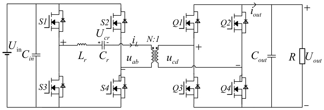
Figure 1 presents a simplified schematic representation of the DBSRC topology. This circuit consists of two full bridges and eight switches S1–S4, Q1–Q4. The input and output voltages are denoted by $U_{in}$ and $U_{out}$, respectively. The resonant current and output current are represented by $i_L$ and $i_{out}$, while $U_{cr}$ corresponds to the switched-capacitor voltage. The load resistance is defined as $R$, and $L_r$, $C_r$, and $C_{out}$ denote the resonant inductor, switched capacitor, and output capacitor. The converter supplies power to a resistive load.

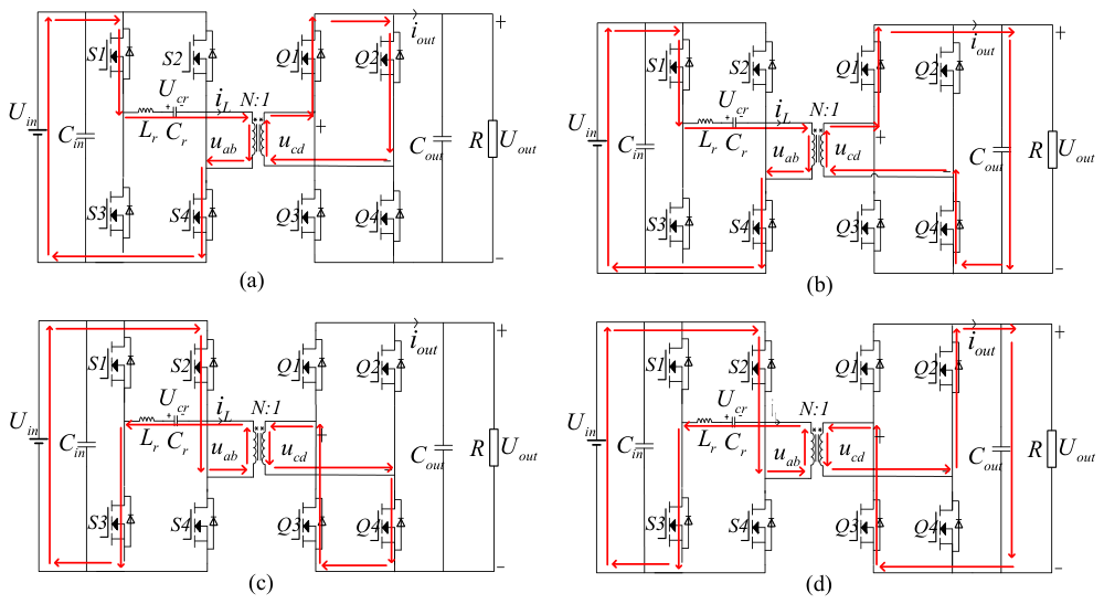
Figure 2 summarizes the four operating modes of the DBSRC. In the first two modes, S1 and S4 remain conducting, while the active secondary-side switches change from Q1–Q2 in Mode 1 to Q1–Q4 in Mode 2. In contrast, Modes 3 and 4 are associated with the conduction of S2 and S3. Specifically, Q3–Q4 conduct in Mode 3, whereas Q2–Q3 conduct in Mode 4 [20]. The complementary switches are kept in the off state during each corresponding interval.

Parasitic components are omitted to facilitate the analysis. As depicted in Figure 2, the converter exhibits four switching modes, each defined by the equations given below [7].

(1) Mode 1

$$\left\{\begin{array}{l}{\dot{i}}_L={\displaystyle \frac{U_{in}-U_{cr}}{L_r}}\\ {\dot{U}}_{cr}={\displaystyle \frac{i_L}{C_r}}\\ {\dot{U}}_{out}=-{\displaystyle \frac{1}{R{C}_{out}}}{U}_{out}\end{array}\right.$$

(1)

(2) Mode 2

$$\left\{\begin{array}{l}{\dot{i}}_L={\displaystyle \frac{U_{in}-U_{out}-U_{cr}}{L_r}}\\ {\dot{U}}_{cr}={\displaystyle \frac{i_L}{C_r}}\\ {\dot{U}}_{out}={\displaystyle \frac{1}{C_{out}}}{i}_L-{\displaystyle \frac{1}{R{C}_{out}}}{U}_{out}\end{array}\right.$$

(2)

(3) Mode 3

$$\left\{\begin{array}{l}{\dot{i}}_L={\displaystyle \frac{-U_{in}-U_{cr}}{L_r}}\\ {\dot{U}}_{cr}={\displaystyle \frac{i_L}{C_r}}\\ {\dot{U}}_{out}=-{\displaystyle \frac{1}{R{C}_{out}}}{U}_{out}\end{array}\right.$$

(3)

(4) Mode 4

$$\left\{\begin{array}{l}{\dot{i}}_L={\displaystyle \frac{U_{out}-U_{\mathrm{i}n}-U_{cr}}{L_r}}\\ {\dot{U}}_{cr}={\displaystyle \frac{i_L}{C_r}}\\ {\dot{U}}_{out}=-{\displaystyle \frac{1}{C_{out}}}{i}_L-{\displaystyle \frac{1}{R{C}_{out}}}{U}_{out}\end{array}\right.$$

(4)

The output voltage is required to track the reference value $U_{ref}$ with a fast dynamic response. The normalized state plane, $U_{out}-i_L$ and $U_{crN}-i_{LN}$ helps to better understand the direct control of the state variables.

3. State-Trajectory Analysis of Dual-Active-Bridge Series Resonant Converter

The approximate natural trajectory of the converter is derived in this section as a basis for constructing the proposed state machine controller.

As indicated in Figure 2, Modes 1 and 3 correspond to intervals in which the series resonant tank has no direct power-transfer path to the load. In these two modes, the applied voltages take two levels, namely $U_{in}$ and $-U_{in}$. As a result, both modes share the same form of state trajectory equation. For clarity, the trajectory corresponding to Mode 3 is derived first, and the solution of Equation (3) can be expressed as follows:

$$i_L=i_{L0}\cos ({\displaystyle \frac{t}{\sqrt{L_r{C}_r}}})+(-U_{in}-U_{cr0})\sqrt{{\displaystyle \frac{C_r}{L_r}}}\sin ({\displaystyle \frac{t}{\sqrt{L_r{C}_r}}})$$

(5)

$$U_{out=}{U}_{out0}{e}^{{\displaystyle \frac{-t}{R{C}_{out}}}}$$

(6)

where $i_{L0}$, $U_{cr0}$, and $U_{out0}$ are the initial values of $i_L$, $U_{cr}$, and $U_{out}$, respectively. By eliminating the time variable in Equation (5), applying a linear approximation near $U_{out}/U_{out0}=1$, after applying trigonometric identities, the relationship between the resonant current and the output voltage can be expressed as follows:

$$i_L=\sqrt{{i_{L0}}^2+{(-U_{in}-U_{cr0})}^2{\displaystyle \frac{C_r}{L_r}}}\sin \left[{\displaystyle \frac{C_{out}R}{U_{out0}\sqrt{L_r{C}_r}}}(U_{out}-U_{out0})+{\tan }^{-1}({\displaystyle \frac{i_{L0}}{U_{in}+U_{cr0}}}\sqrt{{\displaystyle \frac{L_r}{C_r}}})\right]$$

(7)

Using the same analytical procedure, the natural trajectory corresponding to Mode 1 can be obtained, and its mathematical expression is given as follows:

$$i_L=-\sqrt{{i_{L0}}^2+{(U_{cr0}-U_{in})}^2{\displaystyle \frac{C_r}{L_r}}}\sin \left[{\displaystyle \frac{C_{out}R}{U_{out0}\sqrt{L_r{C}_r}}}(U_{out}-U_{out0})+{\tan }^{-1}({\displaystyle \frac{i_{L0}}{U_{cr0}-U_{in}}}\sqrt{{\displaystyle \frac{L_r}{C_r}}})\right]$$

(8)

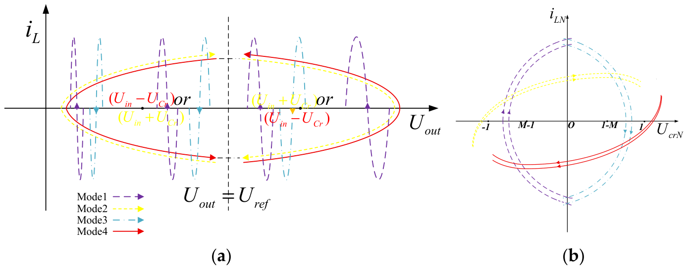
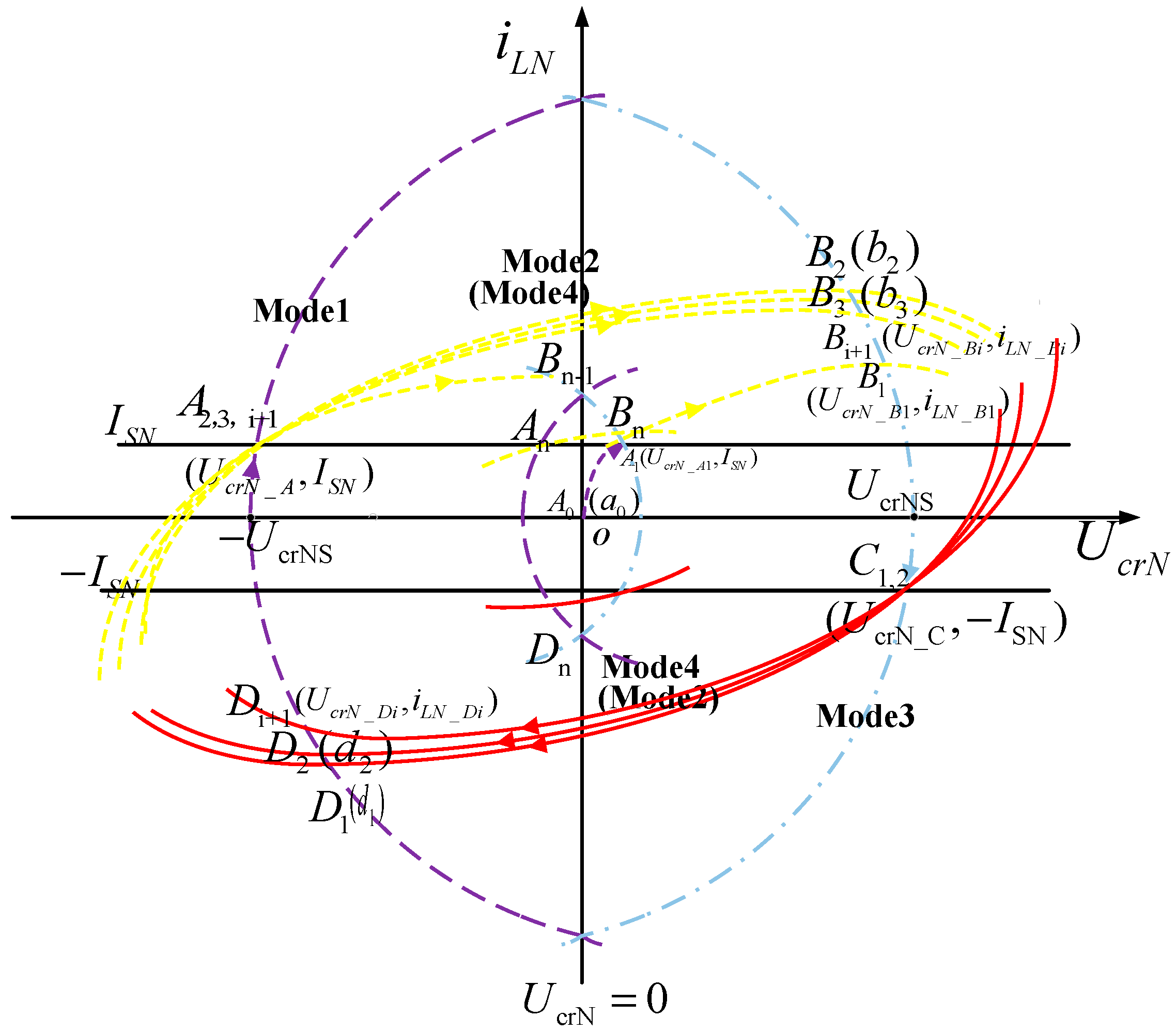
Equations (7) and (8) clearly indicate that the natural trajectories of Mode 3 and Mode 1 in the $U_{out}-i_L$ state plane follow sinusoidal patterns, with amplitudes $\sqrt{{i_{L0}}^2+{(-U_{in}-U_{cr0})}^2{\displaystyle \frac{C_r}{L_r}}}$ and $\sqrt{{i_{L0}}^2+{(U_{cr0}-U_{in})}^2{\displaystyle \frac{C_r}{L_r}}}$, respectively. The red and yellow traces in Figure 3a show that the trajectories of the first and third operating modes shift across the state-plane diagram toward reduced output-voltage values.

The natural trajectory equations for Modes 2 and 4 in the $U_{out}-i_L$ state plane are given below. The load resistance $R$ is considered within the range (0,∞]. The analysis can be simplified when the converter operates without a load. The expression corresponding to Equation (2) is shown below:

$$\left\{\begin{array}{l}{\dot{i}}_L={\displaystyle \frac{U_{in}-U_{out}-U_{cr}}{L_r}}\\ {\dot{U}}_{cr}={\displaystyle \frac{i_L}{C_r}}\\ {\dot{U}}_{out}={\displaystyle \frac{1}{C_{out}}}{i}_L\end{array}\right.$$

(9)

Find the second derivative of $U_{out}$, and then derive the dynamic expression for the output voltage:

$${\ddot{U}}_{out}+{\displaystyle \frac{1}{C_{out}{L}_r}}{U}_{out}={\displaystyle \frac{1}{C_{out}{L}_r}}(U_{in}-U_{cr})$$

(10)

This equation can be further expressed as the natural trajectory in the state plane corresponding to $U_{out}-i_L$:

$${\displaystyle \frac{L_r}{C_{out}}}{i_L}^2+{\left[U_{out}-(U_{in}-U_{cr})\right]}^2={\displaystyle \frac{L_r}{C_{out0}}}{i_{L0}}^2+{\left[U_{out0}-(U_{in}-U_{cr})\right]}^2$$

(11)

By applying a similar analytical method, the natural trajectory associated with Mode 4 in the no-load case can be determined, which is described by the following expression:

$${\displaystyle \frac{L_r}{C_{out}}}{i_L}^2+{\left[U_{out}-(U_{in}+U_{cr})\right]}^2={\displaystyle \frac{L_r}{C_{out0}}}{i_{L0}}^2+{\left[U_{out0}-(U_{in}+U_{cr})\right]}^2$$

(12)

According to Equations (11) and (12), the no-load natural trajectories of Mode 2 and Mode 4 in the $U_{out}-i_L$ state plane can be represented by ellipses centered at points ($U_{in}-U_{cr}$, 0) and ($U_{in}+U_{cr}$, 0), respectively. Furthermore, the semi-major and semi-minor axes of these ellipses depend on the initial values $i_{L0}$ and $U_{out0}$. As illustrated in Figure 2, the series resonant circuit is connected to the load during Modes 2 and 4. As the resonant current rapidly charges or discharges the output capacitor, the output voltage rises or falls, which can be summarized as follows: positive $i_L$ in Mode 2 and negative $i_L$ in Mode 4 increase the output voltage, while negative $i_L$ in Mode 2 and positive $i_L$ in Mode 4 decrease the output voltage. As illustrated in Figure 3a, the natural trajectories corresponding to Mode 2 and Mode 4 follow elliptical paths in the state plane, rotating in the clockwise and counterclockwise directions, respectively. Mode 2 and Mode 4 involve simultaneous charging and discharging of the output capacitor by the power source side and the resonant tank, which expedites the process.

By examining the state plane and its normalized formulation, the proposed state-trajectory control scheme is established. $U_{crN}-i_{LN}$ state plane. The natural trajectories of the four switching modes in the $U_{crN}-i_{LN}$ state plane are described as follows. Using the normalized parameters $Z_r=\sqrt{L_r/C_r}$, $i_{LN}=Z_r{i}_L/U_{in}$, $U_{crN}=U_{cr}/U_{in}$, and $M=U_{out}/U_{in}$, the natural trajectory equations for all four switching modes are obtained.

(1) Mode 1

$${(U_{crN}-1)}^2+{i_{LN}}^2={(U_{crN0}-1)}^2+{i_{LN0}}^2$$

(13)

(2) Mode 2

$${\left[U_{crN}-(1-M)\right]}^2+{i_{LN}}^2={\left[U_{crN0}-(1-M)\right]}^2+{i_{LN0}}^2$$

(14)

(3) Mode 3

$${\left[U_{crN}-(-1)\right]}^2+{i_{LN}}^2={\left[U_{crN0}-(-1)\right]}^2+{i_{LN0}}^2$$

(15)

(4) Mode 4

$${\left[U_{crN}-(M-1)\right]}^2+{i_{LN}}^2={\left[U_{crN0}-(M-1)\right]}^2+{i_{LN0}}^2$$

(16)

where $i_{LN0}$ and $U_{crN0}$ are the initial values of $i_{LN}$ and $U_{crN}$, respectively. Based on Equations (13)–(16), the natural trajectories corresponding to the four switching modes in the normalized $U_{crN}-i_{LN}$ state plane are centered at (1,0), (1 − M,0), (−1,0), and (M − 1,0), as illustrated in Figure 3b. It is worth noting that the radius of each trajectory is determined by the initial state of the series resonant circuit.

By examining the approximate natural trajectories of the converter in the $U_{out}-i_L$ and $U_{crN}-i_{LN}$ state planes, appropriate switching laws can be formulated to shape the state trajectories in these planes, thereby improving the dynamic performance of the converter. Section 4 illustrates representative state trajectories of the DBSRC in both state planes under the proposed control strategy.

4. State-Trajectory Design

Based on the natural trajectories in the two state planes described in Section 3, the state trajectories are constructed to meet the control requirements. The corresponding switching conditions are derived in this section.

In the proposed state-trajectory control, output voltage regulation consists of two stages: a dynamic phase and a steady-state phase.

4.1. Analysis of the Dynamic Regulation Process

When $U_{out}$ < $U_{ref}$, the output capacitor is expected to be charged by the output current $i_{out}$ during the start-up transient, and discharged when $U_{out}$ > $U_{ref}$. A higher mean value of the output current $i_{out}$ is adopted at start-up so that the converter can reach its desired operating condition more rapidly. Mode transitions are triggered by event conditions. The transition from one mode to another takes place once the corresponding event is detected. By employing the state-trajectory regulation strategy developed in this study, a larger average output current can be obtained compared to traditional linear control methods, thereby achieving fast dynamic response during start-up. This is referred to as the dynamic regulation process. A more detailed analysis will be conducted next.

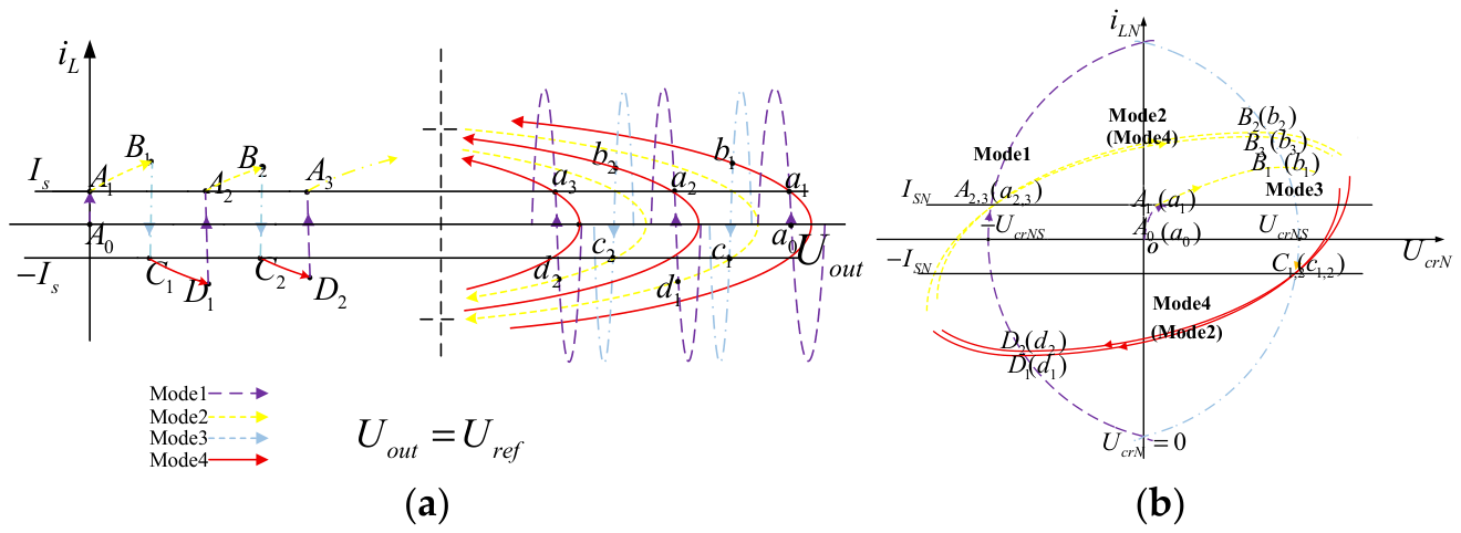
As illustrated in Figure 4a,b, the converter exhibits representative state trajectories when starting from $A_0$ or $a_0$ under the proposed control method. For the case $U_{out}$ < $U_{ref}$, during start-up, a fast transient response is achieved by restricting resonance-current-induced charge depletion in the output-side capacitance during the second and fourth operating stages. That is, undesired reversal of the resonant current must be avoided, with $i_L$ > 0 in Mode 2 and $i_L$< 0 in Mode 4. In addition, Mode 1 or Mode 3 is introduced between Modes 2 and 4, during which the resonant current reverses its polarity rapidly. Consequently, the state trajectories follow a cyclic sequence of “Mode 1, Mode 2, Mode 3, Mode 4, Mode 1…”. In contrast to traditional linear control methods, the output voltage increases almost continuously throughout the switching cycle without noticeable dips (see Figure 4a), resulting in improved dynamic performance. Likewise, when the output voltage is initialized at an arbitrary point satisfying $U_{out}$ > $U_{ref}$. The resonant-branch current is required to remain negative in the second operating interval and positive in the fourth operating interval. The state trajectories follow a cyclic sequence of “Mode 1, Mode 4, Mode 3, Mode 2, Mode 1…”

To achieve the desired state trajectory, Section 4.2 establishes the switching criteria for the developed control strategy. Specifically, during dynamic regulation, the first operating interval is characterized by the positive current limit $I_S$ and the target lower normalized switched-capacitor voltage $-U_{\mathrm{crNS}}$, while the third operating interval is characterized by the negative current limit $-I_S$ and the target upper normalized $U_{\mathrm{crNS}}$.

4.2. Formulation of Switching Criteria

The start-up response is first evaluated from $A_0$, located on the left side of the $U_{\mathrm{out}}-i_{\mathrm{L}}$ state plane, as illustrated in Figure 4a. The converter switches from Mode 1 to Mode 2 once the resonant current in Mode 1 reaches its positive peak $I_S$, which corresponds to point $A_1$. The switching condition is given below:

$$i_{\mathrm{L}}\ge I_S \mathrm{and} U_{\mathrm{out}}\le U_{ref}$$

(17)

The transition criterion between the second and third operating intervals is obtained from the $U_{\mathrm{crN}}-i_{\mathrm{LN}}$ state-plane trajectory shown in Figure 4b, with reference to point, where $I_{SN}$ = $Z_r{I}_S/U_{in}$. Under the resonant-current constraint described above, the system is allowed to enter the third operating interval from the second one only if $i_{LN}$ > 0. Furthermore, As the normalized resonant current falls to zero, the normalized switched-capacitor voltage reaches its peak value. To make the peak value approach the target $U_{crNS}$, the switching condition from Mode 2 to Mode 3 is determined based on Equation (15) and is given below:

$${\left[U_{crN}-(-1)\right]}^2+{i_{LN}}^2\ge {\left[U_{crNS}-(-1)\right]}^2 \mathrm{and} i_{LN}>0$$

(18)

where $U_{crNS}$ represents the prescribed upper bound of the normalized voltage across the switched-capacitor voltage. The method for determining this switching parameter is described in Section 5.2.

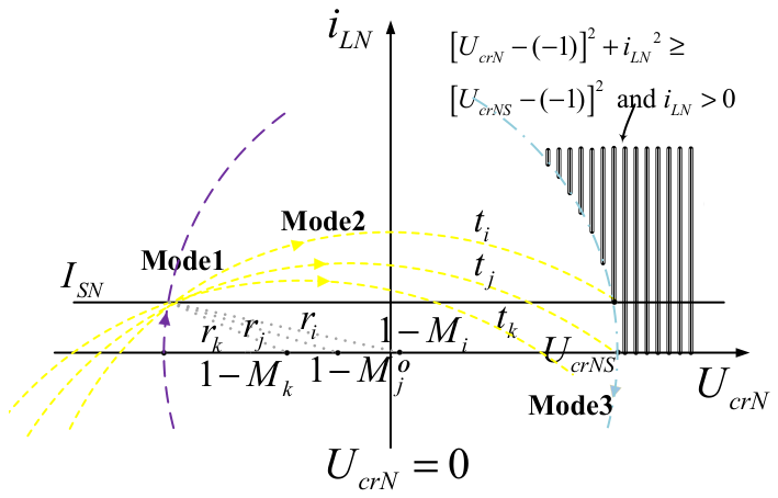
Condition (18) is fulfilled once the trajectory associated with the second operating interval enters the shaded region in Figure 5. In the second operating interval, the trajectory follows a circular path whose center gradually moves toward the origin, with its radius reduced as the converter output voltage falls. In the dynamic regulation stage, the trajectory radii $r_{\mathrm{i}}$, $r_{\mathrm{j}}$, and $r_{\mathrm{k}}$ are mapped to the corresponding conversion ratios $M_{\mathrm{i}}$, $M_{\mathrm{j}}$, and $M_{\mathrm{k}}$, respectively. When the second-interval trajectory stays outside the shaded region a $t_{\mathrm{k}}$, the criterion in Equation (18) is no longer met. An additional transition rule from Mode 2 to Mode 3 is formulated to ensure that $i_{\mathrm{LN}}$ > 0 while preserving the continuity of the switching sequence. The corresponding condition is given below:

$$i_{\mathrm{LN}}\le 0$$

(19)

Point $C_1$ in Figure 4a marks the instant at which the resonant-branch current reaches −$I_S$, thereby initiating the shift from the third operating interval to the fourth. The switching condition is provided below:

$$i_L\le -I_S \mathrm{and} U_{out}\le U_{ref}$$

(20)

The switching rule for the transition from Mode 4 to Mode 1, indicated by point $D_1$, can be obtained using the same analytical procedure employed for the Mode 2–Mode 3 transition. The resulting condition is given below:

$${\left[U_{crN}-1\right]}^2+{i_{LN}}^2\ge {\left[-U_{crNS}-1\right]}^2 \mathrm{and} i_{LN}<0$$

(21)

The additional switching condition is

$$i_{LN}\ge 0$$

(22)

When $U_{ref}$ < $U_{out}$, $a_0$, positioned on the right side of the $U_{out}-i_L$ state plane in Figure 4a, is selected as the initial state for evaluating the start-up behavior. The output voltage settles at the reference level within a few switching cycles.

The above analysis of Modes 2 and 4 is carried out under no-load conditions. Under load conditions, the output voltage drops due to the discharge of the output capacitor by the load current, rather than by the resonant current. Consequently, the damped state-plane trajectory leads to only a modest increase in the duration of the start-up transient.

4.3. Analysis of the Steady-State Regulation Process

In analyzing typical state trajectories, the control strategy transitions to steady-state regulation once the output voltage reaches its reference value, regardless of whether Mode 2 or Mode 4 is the final mode in the dynamic process. The output voltage is then regulated to follow the reference.

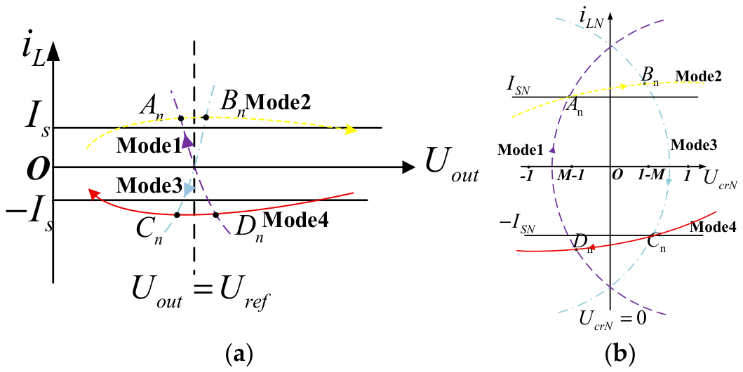
A representative trajectory under steady-state regulation in the $U_{out}-i_L$ plane is depicted in Figure 6a. The trajectory follows a repetitive four-interval pattern: “Mode 1, Mode 2, Mode 3, Mode 4, Mode 1…” The four trajectory segments intersect at $A_n$, $B_n$, $C_n$, and $D_n$. As shown in Figure 6b, the corresponding steady-state trajectory in the $U_{crN}-i_{LN}$ state plane is symmetric about the point (0,0).

In the steady-state regulation stage, the current bounds $I_S$ and $-I_S$ from Section 5.2 are retained so that the resonant current follows the required direction in the second and fourth operating intervals without increasing implementation complexity. Accordingly, Equation (17) governs the transition from the first to the second operating interval, while Equation (20) applies to the transition from the third to the fourth operating interval.

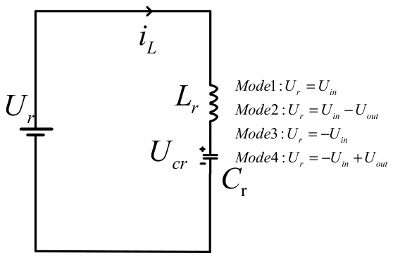
Figure 7 presents a simplified equivalent circuit used to describe the DBSRC converter under steady-state conditions. In this circuit, the source voltage $U_{\mathrm{r}}$ indicates the voltage difference between the midpoint nodes of the left and right full bridges. During switching modes 1–4, the values of $U_r$ are $U_{in}$, $U_{in}-U_{out}$, $-U_{in}$, and $-U_{\mathrm{i}n}+U_{out}$, respectively.

From the equivalent circuit presented in Figure 7, the differential equations describing the system can be established, and their solutions yield the resonant current $i_{\mathrm{L}}$ and the switched-capacitor voltage $U_{cr}$:

$$i_L=\sqrt{{i_{L0}}^2+{({\displaystyle \frac{U_{cr0}-U_r}{Z_r}})}^2}\cos ({\displaystyle \frac{t}{\sqrt{L_r{C}_r}}}+\arctan ({\displaystyle \frac{U_{cr0}-U_r}{Z_r{i}_{L0}}}))$$

(23)

$$U_{cr}=\sqrt{{(U_{cr0}-U_r)}^2+{(Z_r{i}_{L0})}^2}\cos ({\displaystyle \frac{t}{\sqrt{L_r{C}_r}}}-\arctan ({\displaystyle \frac{U_{cr0}-U_r}{Z_r{i}_{L0}}}))+U_r$$

(24)

where $i_{L0}$ and $U_{cr0}$ are the initial values of $i_L$ and $U_{cr}$.

Equation (24) provides the basis for determining the transition criterion between the second and third operating intervals, where $U_{cr0}$ is a known value in steady state, and $i_{\mathrm{L}0}$ can be obtained from $I_T$ as described below. At this step, a recalculated $U_{cr1}$ leads to a switching condition comparable to that applied during the transient state:

$${\left[U_{crN}-(-1)\right]}^2+{i_{LN}}^2\ge {\left[U_{crN1}-(-1)\right]}^2$$

(25)

The Mode 4 to Mode 1 transition condition is determined here by adopting the same methodology previously used for analyzing the Mode 2 to Mode 3 transition. The resulting expression is provided below:

$${\left[U_{crN}-1\right]}^2+{i_{LN}}^2\ge {\left[-U_{crN1}-1\right]}^2$$

(26)

Of course, during Mode 2 and Mode 4, when $U_{out}$ < $U_{ref}$, the control law reverts to the dynamic regulation process.

5. Control Law Design

5.1. State Machine Controller

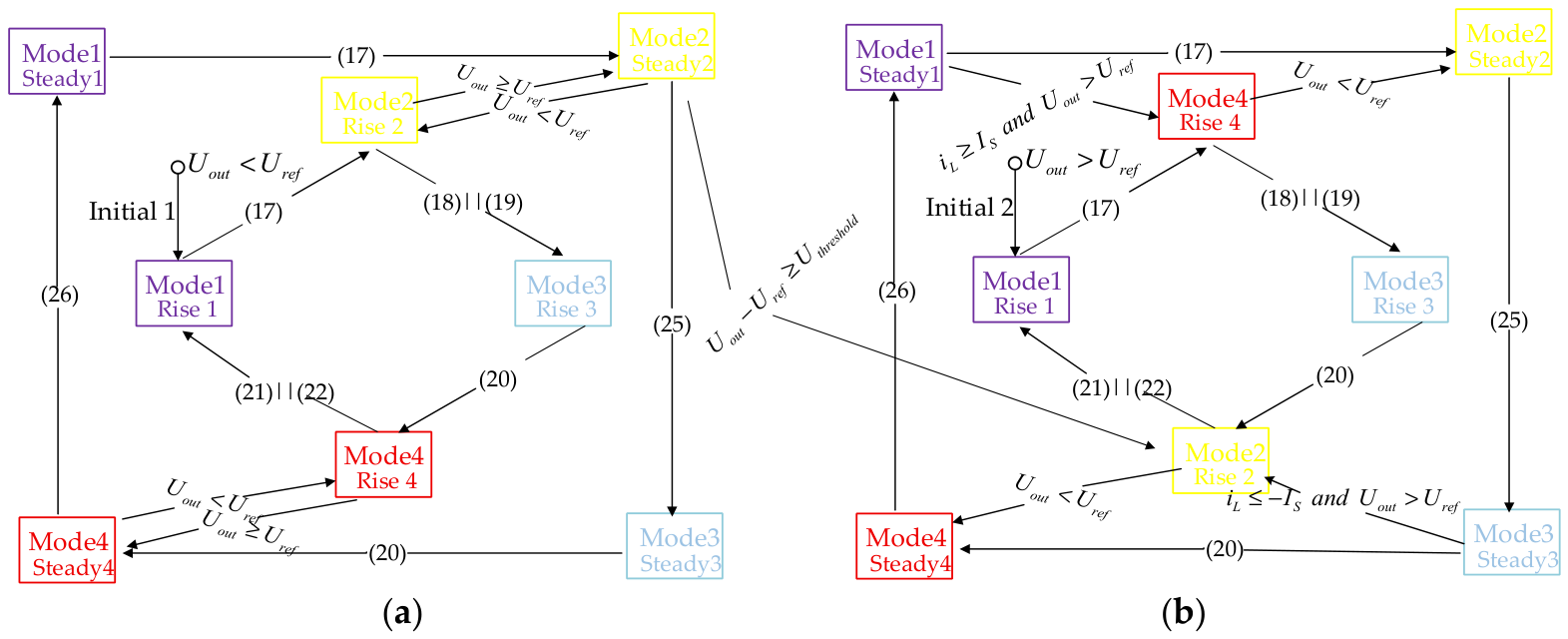
Figure 8 illustrates the controller implemented using a state machine structure. The controller consists of 14 states. Rise 1–4 correspond to the dynamic regulation process when $U_{out}<U_{ref}$, whereas Fall 1–4 are involved when $U_{out}>U_{ref}$. Steady 1–4 belong to the steady-state regulation stage. Each of these states maps to one of Modes 1–4, with the exception of the initial states, Initial 1 and Initial 2.

During the dynamic regulation process, the state machine controller starts from Initial 1 when $U_{out}$ < $U_{ref}$, or from Initial 2 when $U_{out}$ > $U_{ref}$. With the output voltage initially at zero, the control sequence begins in Initial 1 and then transitions to Rise 1. As shown by $A_0$ in Figure 4a, the trajectory originates at (0, 0) and gradually deviates from the horizontal axis. Once the resonant-branch current increases to the prescribed positive threshold $I_{\mathrm{S}}$, State Rise 2 is triggered. During Rise 2, energy is rapidly supplied to the output-side capacitance by the forward resonant-branch current, resulting in a substantial rise in the converter output voltage. Upon meeting switching condition (18) or (19), state Rise 3 is activated. Shorting the series resonant circuit leads to a rapid decline in $i_{\mathrm{L}}$, after which the current reverses polarity. Next, when the negative resonant current reaches its maximum value $-I_{\mathrm{S}}$, state Rise 4 is activated. As in Rise 2, the output voltage increases rapidly as the output capacitor is charged by a negative resonant current. When condition (21) or (22) is satisfied, state Rise 1 is activated again.

Following the iterative process of “Rise 1, Rise 2, Rise 3, Rise 4, Rise 1…”, the trajectory plane of the $U_{out}-i_L$ state rapidly approaches the vertical line $U_{out}=U_{ref}$. When the trajectory crosses the vertical line $U_{out}=U_{ref}$, the state machine controller transitions to steady-state regulation and maintains the trajectory within a stable orbit around the reference point ($U_{\mathrm{ref}}$, 0) through a cyclic sequence of states: “Steady 1, Steady 2, Rise 2, Steady 2, Steady 3, Steady 4, Rise 4, Steady 4, Steady 1…” When the reference voltage drops abruptly, the two states can be linked by $U_{threshold}$, provided that it is greater than the steady-state output voltage ripple.

For the case where the controller starts from Initial 2, a similar analysis can be performed. Under the given initial condition, dynamic regulation proceeds through the repeated state sequence “Fall 1, Fall 4, Fall 3, Fall 2, Fall 1…”, which is the reverse of the state sequence starting from the condition $U_{out}<U_{ref}$. However, when the trajectory enters the steady-state regulation process, the sequence of activated states becomes “Steady 1, Steady 2, Rise 2, Steady 2, Steady 3, Steady 4, Rise 4, Steady 4, Steady 1…”

5.2. Establishment of Switching Parameters

The following expressions define $U_{crNS}$ and $I_S$, which are used as transition thresholds.

Determination of $U_{crNS}$: Figure 4b and Figure 9 indicate that, in the dynamic regulation stage, the normalized voltage across the switched-capacitor voltage should remain within the specified upper and lower bounds:

$$U_{cr}\le U_{rating}$$

(27)

where $U_{rating}$ represents the allowable upper voltage rating of the switched-capacitor voltage, and $U_{\mathrm{crNS}}$ should be designed not to exceed this physical limit.

Furthermore, according to Equations (13)–(16), since the resonant current $i_{\mathrm{LN}\text{\_}\mathrm{Bi}}$ corresponding to point $B_{\mathrm{i}}$ in Figure 9 decreases during the start-up transient, $i_{\mathrm{LN}\text{\_}\mathrm{Bi}}$ can be solved as Equation (28):

$$i_{LN\_Bi}={\displaystyle \frac{{(-2+M_i)}^2{I_{SN}}^2-4(-1+M_i)(1-\sqrt{-{I_{SN}}^2+{(1+U_{CrNS})}^2})(-1+M_i-\sqrt{-{I_{SN}}^2+{(1+U_{CrNS})}^2})}{{(-2+M_i)}^2}}$$

(28)

The peak value of $i_{LN\_B2}$ occurs in the second switching cycle over the regulation interval. Therefore, for $M_2$, Equation (28) is simplified to give $U_{\mathrm{crNS}}$ as:

$$U_{crNS}\le \sqrt{i_{LN\_B2}+1}-1$$

(29)

where $i_{LN\_B2}$ is bounded by the allowable current ratings of the MOSFET and the resonant inductor. Therefore, the switching parameter $U_{crNS}$ can be selected based on Equations (27) and (29).

Choice of $I_{\mathrm{S}}$: the current threshold $I_S$ is specified from the required steady-state switching period $T_{SW}$, and its analytical dependence on $T_{SW}$ is developed in the following equation.

Assuming that the output voltage remains fixed at $U_{\mathrm{out}}$ during steady-state operation, the averaged current delivered to the load can be expressed as a function of the output voltage:

$$i_{out}=U_{out}/R$$

(30)

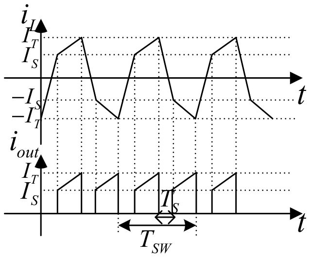
Through the switching actions according to Equations (17), (20), (25), and (26), the switched-capacitor voltage can be balanced at zero, independent of $U_{out}$. During the second and fourth operating intervals, the gradients of the resonant-branch current and output current are set by $U_{out}$, and the associated steady-state current waveforms are illustrated in Figure 10. Through the geometric analysis shown in Figure 10, the following equations are obtained:

$${\displaystyle \frac{I_S+I_T}{T_S}}={\displaystyle \frac{U_{in}}{L_r}}$$

(31)

$${\displaystyle \frac{I_T-I_S}{T_{SW}/2-T_S}}={\displaystyle \frac{U_{in}-U_{out}}{L_r}}$$

(32)

where $I_T$ denotes the resonant current at the transition instant from Mode 2 to Mode 3, and $T_S$ represents the internal phase-shift angle of the secondary-side full bridge. Moreover, the averaged current delivered by the converter can be written as:

$$i_{out}={\displaystyle \frac{(I_S+I_T)(T_{SW}/2-T_S)}{T_{SW}}}$$

(33)

From the above formulas, the relationship between $T_{SW}$ and $I_T$ can be derived:

$$T_{SW}={\displaystyle \frac{2L_r}{{U_{in}}^{2}R(U_{in}-U_{out})}}(U_{out}(4{U_{in}}^2-4U_{in}{U}_{out}-U_{in}{I}_{S}R+{U_{out}}^2)+(2U_{in}-U_{out})\sqrt{4{U_{in}}^2{U_{out}}^2+{U_{in}}^2{I_S}^2{R}^2-4U_{in}{U_{out}}^3-2U_{in}{U_{out}}^2{I}_{S}R+{U_{out}}^4})$$

(34)

$$I_T={\displaystyle \frac{-U_{out}(U_{out}-2U_{in})}{R{U}_{in}}}+{\displaystyle \frac{\sqrt{{U_{out}}^4-4{U_{out}}^3{U}_{in}-2{U_{out}}^{2}R{U}_{in}{I}_S+4{U_{out}}^2{U_{in}}^2+R^2{U_{in}}^2{I_S}^2}}{R{U}_{in}}}$$

(35)

Equation (34) then provides the required value of $I_{\mathrm{S}}$ for the specified switching period $T_{\mathrm{SW}}$.

5.3. Determination of Switching Parameters

The proposed controller is affected by resonant-parameter uncertainty mainly through the calculated natural trajectories and the relationship between $I_{\mathrm{S}}$ and the steady-state switching period. If $L_r$ or $C_r$ deviates from its nominal value, the actual resonant frequency and trajectory radius change, which may shift the exact switching instants. However, the controller makes switching decisions using measured state variables rather than a purely open-loop timing sequence. Therefore, moderate parameter deviations primarily modify the duration of each mode rather than destroying the state-machine sequence. In practice, sufficient design margins should be reserved for $U_{\mathrm{crNS}}$ and $I_{\mathrm{S}}$ so that capacitor-voltage and current-stress limits are not reached under parameter tolerances.

Sensing noise and digital quantization can cause undesired state toggling when the measured trajectory is very close to a switching boundary. This issue can be mitigated by adding a small hysteresis band, a minimum state-holding time to the measured variables. Input-voltage variations influence the conversion ratio M and the normalized switched-capacitor voltage. Hence, $U_{\mathrm{in}}$ should be measured or updated in the normalization process when the converter operates over a wide input-voltage range. Load disturbances are considered by updating the load estimate R, which allows the steady-state switching condition to adapt to the actual load. These measures improve the practical robustness of the proposed FSM implementation while maintaining its simple control structure.

6. Experimental Verification and Analysis

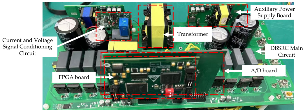
Based on the above analysis, to further evaluate the performance of the developed control scheme, a DBSRC experimental platform was built as shown in Figure 11. The platform mainly includes: the main circuit of the DBSRC, the signal acquisition circuit, the FPGA control circuit, and the gate drive circuit. The operating principle of the system is as follows: The main circuit of the converter operates, generating signals for the resonant current $i_L$, output voltage $U_{out}$, switched-capacitor voltage $U_{cr}$, and output current $i_{out}$. These signals are converted into digital signals by the signal acquisition circuit. The FPGA main controller, based on the finite-state machine control algorithm shown in Figure 8, outputs the switching signals for the converter. Ultimately, the switching signals are reinforced by the gate drive circuit to provide the required driving capability for the MOSFETs in the main circuit. The main parameters used in the experimental setup are summarized in

Table 1. System experimental parameters.

Parameters	Numerical Value
Output voltage reference value $(U_{ref}$)	14.5 V
Input voltage $(U_{in}$)	30 V
Resonant inductor $(L_r$)	27 $\mathsf{\mu }\mathrm{H}$
Switched capacitor $(C_r$)	9.4 $\mathsf{\mu }\mathrm{F}$
Output capacitor $(C_{out}$)	150 $\mathsf{\mu }\mathrm{F}$
Load (R)	3 $\Omega$–6 $\Omega$

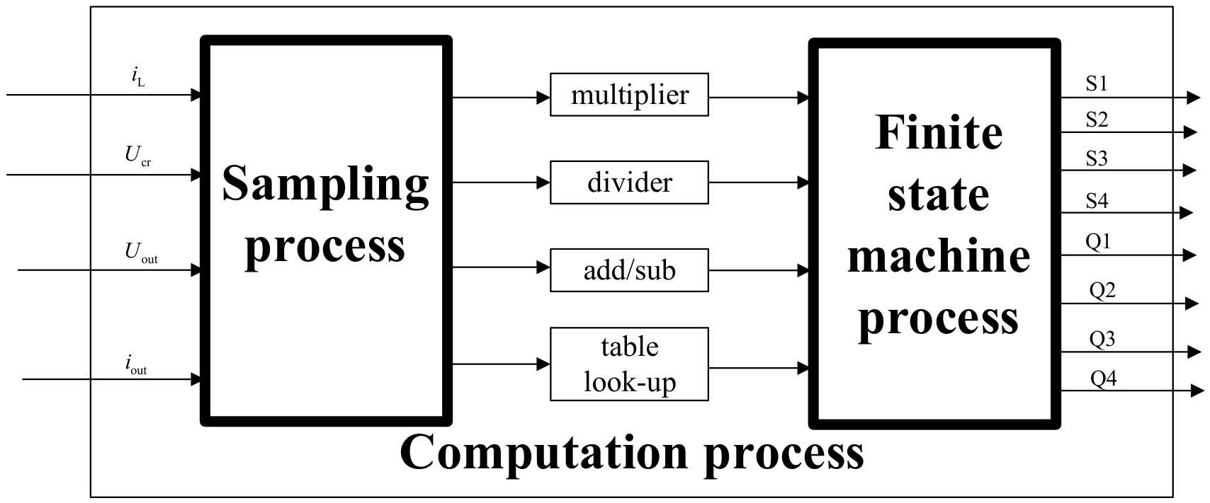
. Figure 12 shows the FPGA implementation structure of the controller, which mainly consists of three parts: a sampling module, a computation module, and a finite-state machine module.

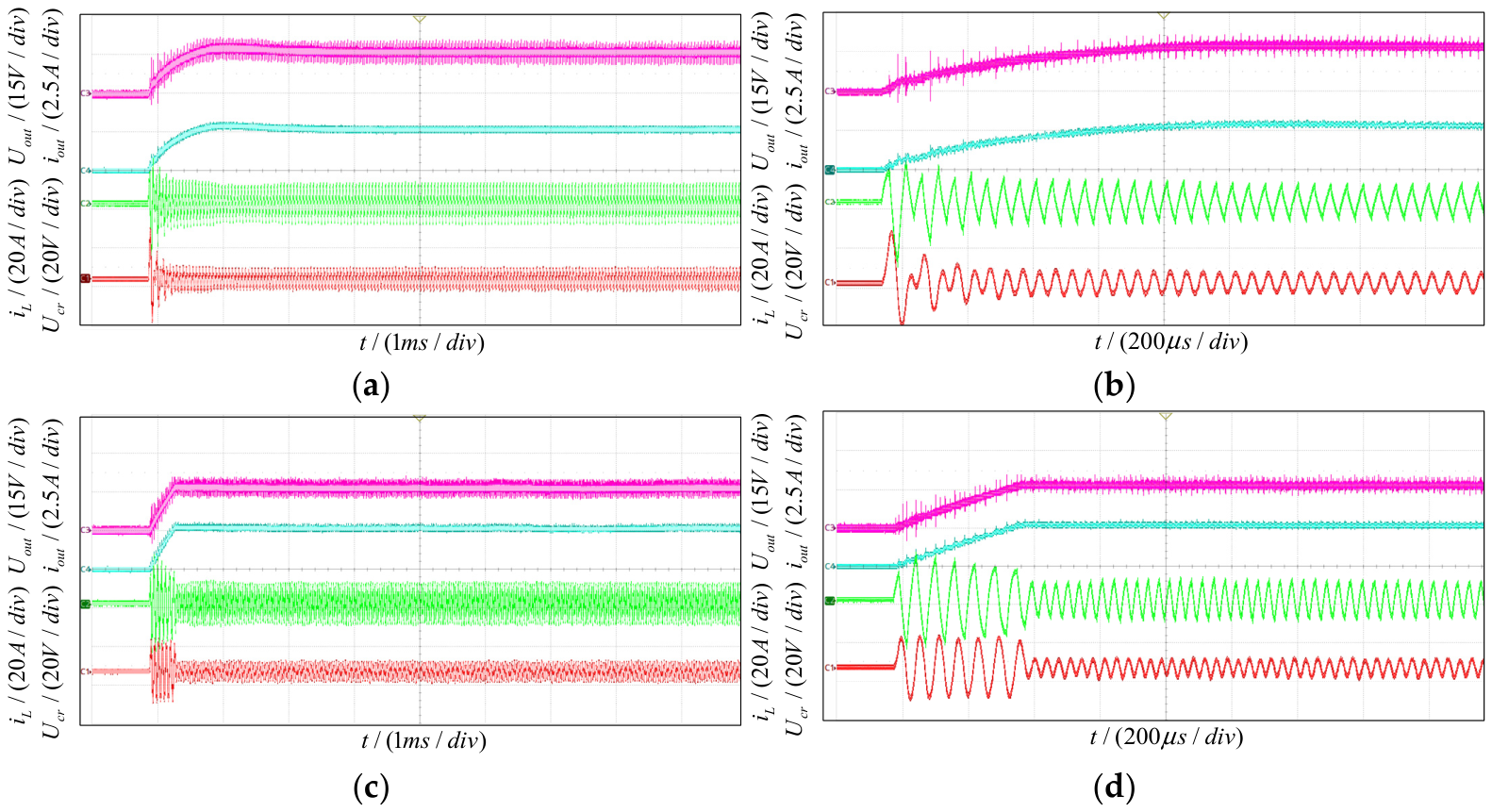
The start-up transient responses from zero output voltage are experimentally compared in Figure 13 for conventional PI regulation and the trajectory-guided control scheme developed in this study.

For traditional PI control, the switching period $T_{SW}$ = 33.3 $\mathsf{\mu }\mathrm{s}$. As shown in Figure 13a, under a 6 $\Omega$ load condition, the rise time of the output voltage start-up transient response is approximately 1.9 ms, equivalent to about 57 switching cycles, and overshoot is observed. Figure 13b shows the detailed waveform of the first 2 ms of the start-up transient corresponding to Figure 13a. As shown in the figure, the output voltage decreases markedly within each switching period, while the net voltage rise achieved per cycle remains limited, thereby resulting in a prolonged start-up process. In fact, with the PI control method, adjusting its parameters cannot significantly improve the dynamic performance of the converter.

Under the trajectory-guided control scheme, $U_{crNS}$ is set to 0.91, and the steady-state switching period is selected as 37.2 $\mathsf{\mu }\mathrm{s}$. According to Equation (34), $I_S$ is calculated to be 4 A. Figure 13c shows the start-up transient response waveforms of the DBSRC under the proposed state-trajectory control method with a load resistance of 6 $\Omega$. In the figure, oscilloscope channels C1 to C4 sequentially display the waveforms of the resonant current $i_L$, switched-capacitor voltage $U_{cr}$, output current $i_{out}$, and output voltage $U_{out}$. The measured results indicate that the developed control scheme provides an overshoot-free start-up response for the dual-active-bridge series-resonant converter, with the output voltage rising to its reference value within approximately 380 $\mathsf{\mu }\mathrm{s}$. Figure 13d shows the detailed waveform of the first 2 ms of the start-up transient corresponding to Figure 13c. It can be observed from the figure that there is no significant voltage drop during the output voltage rise phase, and the start-up transient reaches steady state with the output voltage tracking the reference voltage after only about seven complete switching cycles. The steady-state ripple amplitude is approximately 312 mV. The converter exhibits superior transient performance under trajectory-guided control compared with the PI-based approach.

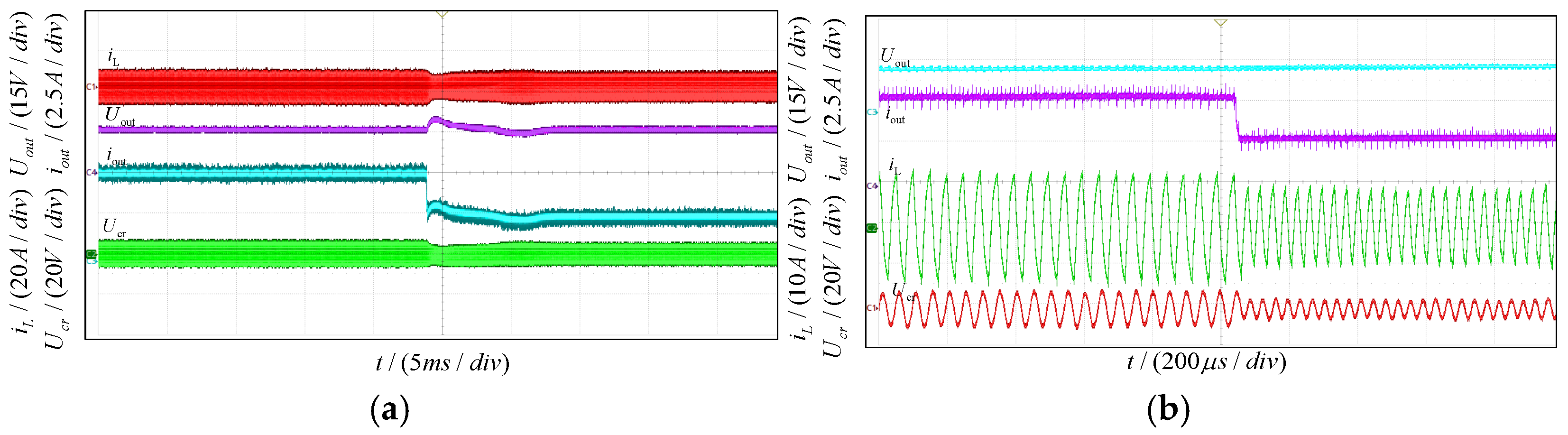
The experiment tested the dynamic response of the converter under two control methods when the load changed from 3 $\Omega$ to 6 $\Omega$. The experimental waveforms in Figure 14 indicate that, under PI control, the load-step change simultaneously causes a sudden change in the load current. At this point, the output capacitor undergoes dynamic charging, causing the output voltage to deviate from the set value. A step decrease in load leads to a significant overshoot in the output voltage. The controller restores the output voltage to steady-state operation in approximately 10 ms. By comparison, the response in Figure 14b demonstrates that the trajectory-guided scheme enables overshoot-free settling of the output voltage within one switching event. Compared to PI control, the converter employing the proposed state-trajectory control method exhibits a faster load response speed.

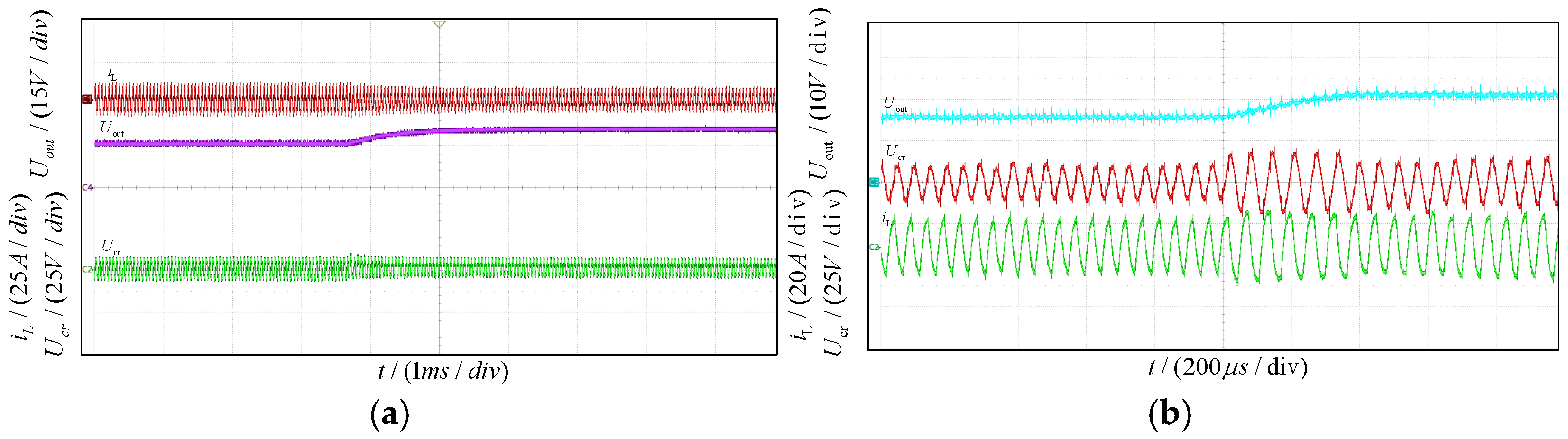
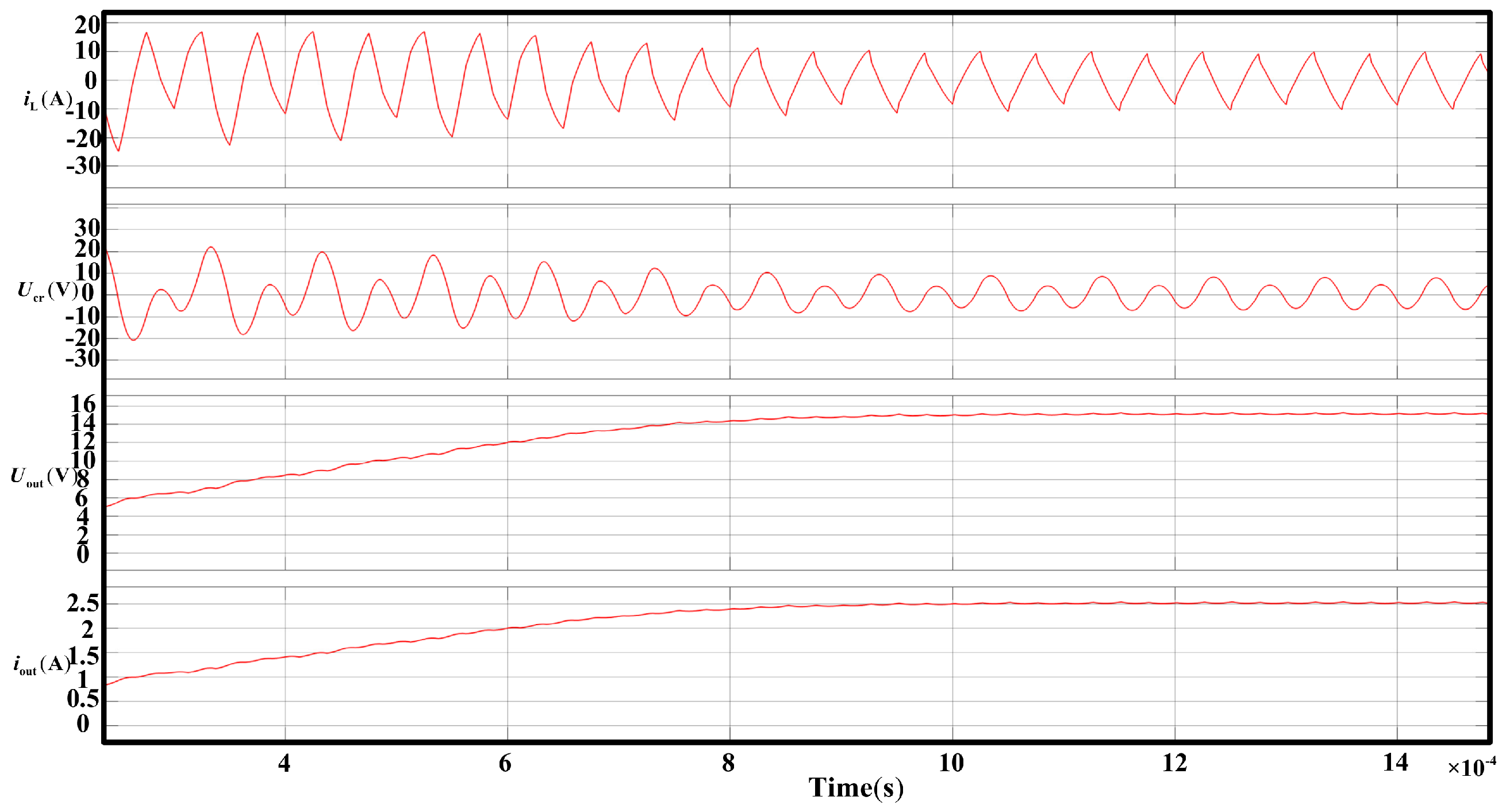
Figure 15 shows that in the case of a reference-voltage step change from 15 V to 20 V, the state-trajectory control exhibits a faster response speed than PI control, demonstrating better dynamic performance. Figure 16 shows the experimental waveforms of transient start-up under model predictive control. It can be seen that under a 6 Ω load, the rise time of the output voltage start-up transient response is approximately 0.9 ms, which is still insufficient compared to the trajectory control method under the same experimental conditions. To quantitatively evaluate the improvement in dynamic characteristics, several performance indicators are extracted from the experimental waveforms, including rise time, number of switching cycles required to reach steady state, overshoot behavior, load-step recovery time, and reference-tracking response. The comparison between the conventional PI controller and the proposed state-trajectory control method is summarized in

Table 2. Dynamic-performance comparison between PI control and the proposed state-trajectory control.

Test Condition	PI Control	Proposed State-Trajectory Control	Performance Comparison
Start-up under 6 Ω load	Rise time about 1.9 ms; about 57 switching cycles; overshoot observed	Rise time about 380 μs; about 7 switching cycles; no overshoot	Rise time reduced by about 80%; switching cycles reduced by about 88%
Output-voltage behavior during start-up	Noticeable voltage drop appears within each switching period	Output voltage rises almost monotonically and reaches the reference without obvious drop	Undesired output-capacitor discharge is suppressed
Load step from 3 Ω to 6 Ω	Obvious overshoot; recovery time about 10 ms	Returns to steady state after one switching action; no visible overshoot	Faster disturbance rejection and smaller voltage deviation
Reference step from 15 V to 20 V	Slower response to the new reference	Faster tracking of the new reference voltage	Improved reference-tracking transient performance
Steady-state ripple under 6 Ω load	Not quantified from the PI waveform	Approximately 312 mV	Stable steady-state tracking after fast start-up

.

7. Conclusions

This work develops a trajectory-guided control scheme for the DBSEC using a finite-state-machine framework. By analyzing the two state planes, the switching operating modes of the converter can be revealed more clearly, and a descriptive model of its operational behavior can be established within a geometric framework. The converter exhibits improved transient performance under the developed control scheme compared with conventional linear control approaches. Through regulation with a few switching actions, fast transient response can be achieved under conditions such as start-up processes, reference-voltage variations, and sudden load changes, while effectively suppressing output overshoot. The measured results demonstrate the effectiveness of the developed control scheme. Under a 6 $\Omega$ load, the start-up rise time was reduced from about 1.9 ms with PI control to about 380 $\mathsf{\mu }\mathrm{s}$, while the number of switching cycles required to reach steady state decreased from approximately 57 to about 7. In addition, the proposed method suppressed the start-up overshoot and maintained stable steady-state operation. During the 3 $\Omega$ o 6 $\Omega$ load-step test, the output voltage recovered after one switching action, whereas the PI controller required nearly 10 ms and exhibited obvious overshoot. These results confirm that the proposed state-trajectory control method provides faster transient response and better voltage regulation than conventional PI control.