Impact of Inertia Variability on the Transient Stability of Interconnected Power Systems: A Methodology for the Estimation of Transient Stability Margins

Abstract

The aim of this paper is to study the impact of the variability of inertia of interconnected electrical systems on transient stability. In the first part of the paper, after formulating the transient stability problem as a boundary value problem, we demonstrate how to evaluate the transient stability margin, considering the impact of the randomness of inertia, with reference to a single area connected to an infinite power grid. In the second part of the paper, we determine the distributional properties of the transient stability margin for two interconnected areas, considering the correlation of the area’s inertias, described as random variables. To demonstrate the robustness of the procedure, two case studies are analyzed. In the first case, the random variables are described as correlated lognormal random variables, while in the second they are considered as correlated gamma random variables. The numerical analyses reported in the final part of the paper show an almost linear dependence of transient stability margin from inertia while correlation coefficient affects mainly the transient stability random variable’s dispersion rather than its magnitude. Some useful considerations are performed regarding the applicability and validity of the linearized probabilistic method instead of the Monte Carlo method. The Monte Carlo method allows considering the non-linearity of the model, which is more pronounced in the tails. This could affect, in some critical cases, the priority of access to production in the logic of the free market. In such a case, greater accuracy allows for a more transparent mechanism of access to production.

1. Introduction

The progressive reduction in rotational inertia in the power grids, resulting from the increasing inverter-based generation, represents a significant challenge to power system security, as already expected by European Network of Transmission System Operators for Electricity (ENTSO-E) [1], which proposed several measures to mitigate the problem in [2]. The inertia reduction is the subject of extensive discussion in contemporary research: ref. [3] discusses various methodologies to maintain power system stability increasing inertia, ref. [4] provides some tools for analysis of low-inertia power systems security, ref. [5] analyses the stability support provided by utilizing the fast response capability of converter to provide virtual inertia and ref. [6] shows the inertia level dependence from location in the power system.

Since the electrical power system is a complex electromechanical system, inertia is a central variable for the analysis of stability and frequency regulation [7]. The core of the modeling is the d’Alembert equation whose essential parameter is inertia. The massive and widespread penetration of modern electricity production systems replacing conventional rotational generation systems (energy transition) has led to a high variability of the inertia parameter [8], at an area level and also at a global level, requiring its measure and estimation at low [9], medium and high voltage power grid, and estimation of its effects on power system transient stability [10]. The decrease in the inertia of power systems after the grid integration of a high proportion of renewable energy sources connected to the power grid through power electronic inverters introduces faster dynamics than conventional controllers [11]. This could cause outage accidents such as those which occurred in Britain and Texas, as described in [8].

A critical aspect of both the planning and operation of electrical power systems is certainly that of the evaluation of transient stability margins (TSMs) [12]. Inertia plays a fundamental role in the variation in the rotor motions of machines [13] and their parameters [14], and it is important to identify the variation characteristics of the maximum transmissible power as a function of the inertia variation interval. It is appropriate to say that inertia is a random quantity and, therefore, the most rigorous way to deal with this problem is to resort to appropriate probabilistic methodologies.

In a previous work [11], some of the authors described the inertia of the system in a probabilistic way by introducing the so-called “Renewable Energy Source Share” (RESS) which is a function of both the renewable energy and conventional energy amount. In [11], based on real data, these quantities were described through statistically independent lognormal random variables.

Borrowing this type of approach, like in [15], in this work first, with reference to an area connected to the rest of the network via a double three-phase line, the transient stability margin is described in a probabilistic way in the face of a single-phase short-circuit to earth with successful reclosing of the line affected by the fault; secondly, unlike [15], in order to exam a more general scenario, such as that with renewable distributed energy resources (DERs), the same approach is opportunely applied to two-area of the power system connected to each other, and TSM has been evaluated considering the interaction between two different areas characterized by their own inertia for different fault types. Moreover, in this investigation, an inertia correlation between two areas is considered according to appropriate assumptions related to two cases: the inertia is assumed as multivariate lognormal or multivariate gamma random variables are chosen because the parameters of the gamma distribution allow great flexibility in adapting to a wide variety of histograms related to real data. The authors proposed an optimization procedure to generate the multivariate gamma distribution. The inertial contribution of each area is used to evaluate the equivalent total inertia of the system. Other papers analyzing transient stability of a power system with a two-area model, such as in [16], without considering its dependence on inertia of areas and its probabilistic values. In [17] the same model is used for evaluation of the so-called “probability of transient stability” obtained assuming a normal distribution of rotor angle displacement due to the cumulative effect of the generic random disturbance.

The stability problem, modeled as a boundary value problem, allows us to find the value of the maximum transmittable power for each given value of inertia applying the equal area criterion (EAC) [18]. With a classic Monte Carlo procedure, it is possible to evaluate the approximation of the probability density function (PDF) of the stability margin. This type of approach is certainly very useful in the planning phase and for understanding the extent of the impact of inertia on the stability margin.

Other fast estimation methods of TSM are presented in the literature as in [19], in which the TSM is evaluated in power system with uncertainty due to high-level penetration of wind generation using a single machine infinite bus (SMIB) model and unscented transformation.

In Section 2 of this paper the theoretical development for TSM evaluation is described for a SMIB and the model is extended for a power system constituted of two areas, while, in Section 3, the probabilistic methodology for TSM evaluation and the original sensitivity analysis of TSM dependence on inertia for the two-area model are reported. Section 4 focuses on the linear dependence of TSM on inertia, while Section 5 shows some probabilistic analyses regarding TSM evaluation in two-area model for specific case studies considering the innovative analysis of its dependence on a correlation between inertia variables of two areas of the power system.

2. Stability Margins Evaluation as a Boundary Value Problem

In this paper, the problem of determining transient stability is solved by formulating an appropriate boundary value problem. Following the contingency, the electrical system appears as a sequence of dynamic systems different in terms of configuration. The transient stability margin is defined as the maximum power that can be delivered by the prime mover such that, given the fault clearance time ${\Delta t}_{cl}$ and the reclosing time ${\Delta t}_r$, stability is regained. This value can therefore be determined by requiring the dynamic system to reach the post-fault unstable equilibrium point at the end of the trajectory. As will be seen below, this unknown is determined based on the application of the area criterion, which is essentially an energy criterion based on an integral formulation. To use the criterion as a nonlinear algebraic equation with a single unknown, the entire trajectory of the dynamic system is expressed as a function of the initial condition using the explicit Euler method. Obviously, the electrical quantities are also expressed as a function of the single unknown, with the reactive power delivered being the parameter.

2.1. Formulation of the Problem for One Machine Connected to Infinite Bus

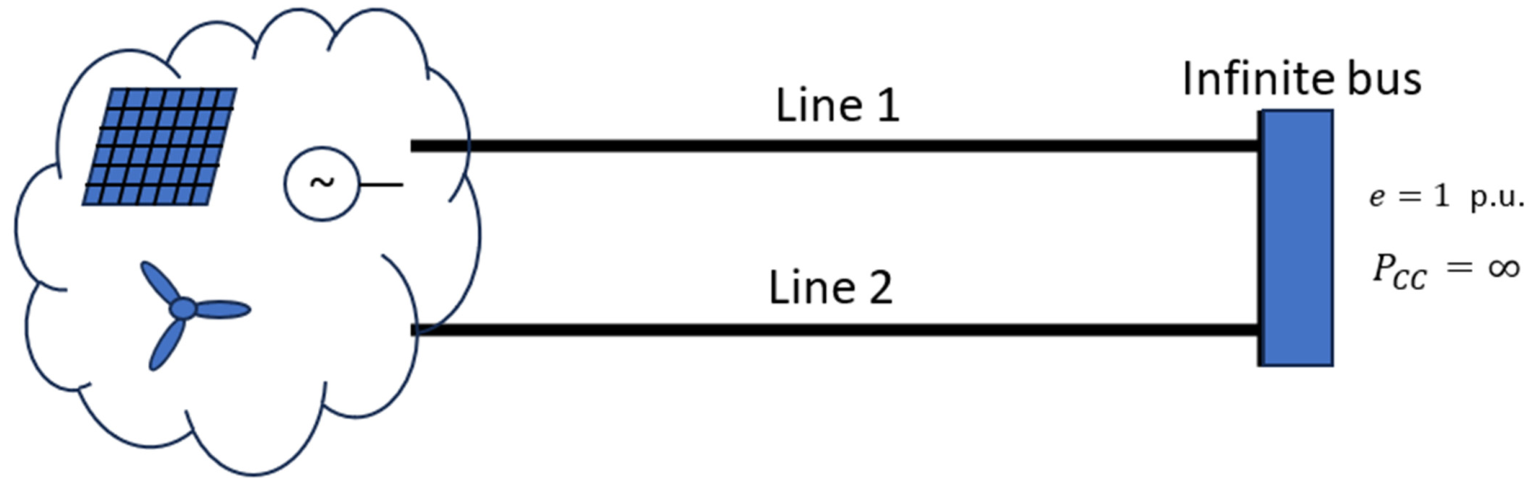
In this section we intend to show the method used to evaluate TSM. To this end, without loss of generality, explicit reference will be made to an area of the electrical system connected via passive double three-phase line to a network bus assumed to have infinite short-circuit power (infinite power bus $P_{CC}=\infty$): Figure 1. Without loss of generality, the voltage magnitude ($e$) of this bus is supposed to be equal to 1 p.u.

The area of the electrical power system modelled is a multi-generators power system region with conventional and renewable generators. The conventional synchronous generators are characterized by high mechanical inertia, while the renewable power generation is a stochastic process and could be not able to support power system during frequency excursions. The randomness of the value of power generated by renewable sources leads, as already mentioned, to the consequent randomness of the equivalent area inertia.

For this investigation the area is modelled as a single equivalent generator delivering power through a transformer with its reactance $x_{tran}$ (SMIB or OMIB—one machine infinite bus—model). The equivalent generator is assumed to have a constant electromotive force and its own direct and inverse transient reactances $x_d^{\prime }$ and $x_i$ (the last assumed equal to subtransient reactance $x_d^{″}$). Each single-circuit three-phase line of length $l$ is characterized by its direct and zero reactance ($x_l$ and $x_{l0}$, respectively).

The variability of electric power is described, as made in the relevant technical literature, by a sinusoidal law as a function of the rotor position, with a maximum amplitude dependent on a suitable equivalent reactance which in turn depends on the various phases of the transient, that is, whether it occurs during the fault, the elimination of the fault, and the subsequent reclosing:

$$p_{e,max}={\displaystyle \frac{e_t^{\prime }e}{x_{eq}}}$$

(1)

where $e_t^{\prime }$ is the transient electromotive force of the equivalent generator and $x_{eq}$ is the equivalent reactance of the switching system according to

$$x_{eq}=\left\{\begin{array}{c}\begin{array}{cc}{x}_{tot},\hfill & \hfill t=0\\ x_{totf},\hfill & \hfill 0<t\le {\Delta t}_{cl}\end{array}\\ \begin{array}{cc}{x}_{totr},\hfill & \hfill {\Delta t}_{cl}<t\le {\Delta t}_{cl}+{\Delta t}_r\\ x_{tot},\hfill & \hfill t>{\Delta t}_{cl}+{\Delta t}_r\end{array}\end{array}\right.$$

(2)

where $x_{tot}$, $x_{totf}$ and $x_{totr}$ are the values assuming by $x_{eq}$ in steady-state condition, during the fault and reclosing time.

It is a matter of evaluating the equivalent impedance in the positive sequence, which is responsible for the active power transfer mechanism, that changes because of the fault and subsequent elimination and reclosing.

For sake of illustrations, in the following the single-phase short-circuit to earth is examined. The equivalent reactance of system in steady-state condition (pre-fault steady state) $x_{tot}$ is

$$x_{tot}=x_{tran}+x_d^{\prime }+{\displaystyle \frac{x_l}{2}}$$

(3)

At time $t$ = 0, from the pre-fault stable equilibrium state, the power transfer mechanism is affected by a random single-phase short-circuit to earth which occurred at a random distance $l_1$ from transformer busbar on one single-circuit of a double three-phase line.

It is useful to define the following reactances corresponding to the two sections of the transmission line:

$$x_{l1}=x_l{\displaystyle \frac{l_1}{l}}, x_{l2}=x_l\left(1-{\displaystyle \frac{l_1}{l}}\right)$$

(4)

$$x_{l01}=x_{l0}{\displaystyle \frac{l_1}{l}}, x_{l02}=x_{l0}\left(1-{\displaystyle \frac{l_1}{l}}\right)$$

(5)

for direct and zero sequence respectively.

During the fault time interval, the equivalent reactance of system, as far as the active power is concerned, becomes

$$x_{totf}=x_{tot}+{\displaystyle \frac{\left(x_d^{\prime }+x_{tran}+\frac{x_{l1}}{2}\right)\frac{x_{l2}}{2}}{\frac{x_{l1}{x}_{l2}}{2x_l}+x_g}}$$

(6)

where the equivalent fault reactance $x_g$ is

$$x_g=x_i+x_0$$

(7)

with

$$x_i={\displaystyle \frac{x_{l1}{x}_{l2}}{{2x}_l}}+{\displaystyle \frac{\frac{x_{l2}}{2}\left(x_d^{″}+x_{tran}+\frac{x_{l1}}{2}\right)}{x_d^{″}+x_{tran}+\frac{x_l}{2}}}$$

(8)

and

$$x_0={\displaystyle \frac{x_{l01}{x}_{l02}}{{2x}_{l0}}}+{\displaystyle \frac{\frac{x_{l02}}{2}\left(x_{tran}+\frac{x_{l01}}{2}\right)}{x_{tran}+\frac{x_{l0}}{2}}}$$

(9)

The faulted single-circuit of double three-phase line supposed to be cleared by its circuit breaker at $t={\Delta t}_{cl}$: the system delivers power through the unfaulted line. Therefore, the equivalent reactance is

$$x_{totr}=x_{tran}+x_d^{\prime }+x_l$$

(10)

Successively the circuit breaker implements the fast reclosing at time $t={\Delta t}_{cl}+{\Delta t}_r$ which is supposed to be successful. Then the equivalent reactance of system will be equal to equivalent reactance of system in steady-state condition $x_{tot}$.

Power system stability can be compromised by various types of faults. The proposed TSM assessment methodology can be applied to each of these by making appropriate modifications to the system reactance formulation. Therefore, to test the robustness of the methodology, three-phase, two-phase, and two-phase-to-ground faults were also considered. In

Table 1. Reactances expression for the various fault typologies.

Earth Fault Type	${\mathit{x}}_{\mathit{t}\mathit{o}\mathit{t}\mathit{r}}$	${\mathit{x}}_{\mathit{t}\mathit{o}\mathit{t}\mathit{f}}$	${\mathit{x}}_{\mathit{g}}$
Single-phase	$x_{totr}=x_{tran}+x_d^{\prime }+x_l$	$x_{tot}+{\displaystyle \frac{\left(x_d^{\prime }+x_{tran}+\frac{x_{l1}}{2}\right)\frac{x_{l2}}{2}}{\frac{x_{l1}{x}_{l2}}{2x_l}+x_g}}$	$x_i+x_0$
Two-phase			${\displaystyle \frac{x_i{x}_0}{x_i+x_0}}$
Two-phase ground			$x_i$
Three-phase			0

the expressions of the different reactances are reported for the various fault typologies.

The stability margin is defined as the maximum value of the power $p_m$ such that, in the event of a given fault and for given values of the fault clearing time ${\Delta t}_{cl}$ and reclosing time ${\Delta t}_r$, the condition of stability is still maintained. This value corresponds to the equality of the accelerating and decelerating areas at the unstable equilibrium point, by applying the well-known equal area criterion to the electromechanical transient dynamic model of the generator. This model, by neglecting the damping torque can be expressed as

$$\left\{\begin{array}{c}{\displaystyle \frac{d\delta }{dt}}=∆\omega =\omega -{\omega }_0\\ {\displaystyle \frac{d∆\omega }{dt}}={\displaystyle \frac{{\omega }_0}{T_a}}\left(p_m-p_e\right)={\displaystyle \frac{{\omega }_0}{T_a}}\left(p_m-p_{e,max}sen\delta \right)={\displaystyle \frac{{\omega }_0}{T_a}}\left(p_m-{\displaystyle \frac{e_t^{\prime }e}{x_{eq}}}sen\delta \right)\end{array}\right.$$

(11)

where

• $\delta$ is the angular position of the synchronous machine rotor relative to a synchronously rotating reference frame;
• $\omega$ and ${\omega }_0$ are actual and rated values, respectively, of angular speed of equivalent machine expressed in [rad/s];
• $T_a$ is the mechanical starting time of the equivalent generator [s];
• $p_m$ and $p_e$ are the mechanical and active electric power, respectively, [p.u.].

The electromotive force $e_t^{\prime }$, see Equation (13), can be expressed as a function $g_1(p_0)$ of active power delivered to the network at steady by infinite bus (the subscript 0 is related to steady state):

$$p_0=p_{m0}={\displaystyle \frac{e_t^{\prime }e}{x_{eq}}}sen{\delta }_0$$

(12)

$$e_t^{\prime }=\left|e+j{x}_{eq}{\displaystyle \frac{p_0\left(1-j\tan \varphi \right)}{e}}\right|=g_1(p_0)$$

(13)

where $\cos \varphi$ is the power factor, which can be handled as a parameter.

The steady state angle ${\delta }_0$ can be expressed as function $g_2(p_0)$:

$${\delta }_0=arcsen{\displaystyle \frac{p{x}_{eq}}{e_t^{\prime }e}}=arcsen{\displaystyle \frac{p{x}_{eq}}{g_1(p_0)e}}=g_2(p_0)$$

(14)

The dynamics of the electromechanical system correspond to a switching system, that is, to a second-order dynamic system with time-variable parameters. However, the initial and final conditions of the system must correspond to equilibrium conditions. The initial condition is characterized by $∆\omega \left(0\right)=0$ and $\delta \left(0\right)={\delta }_0$, for the end one $∆\omega =0$ and $\delta ={\pi -\delta }_0$. Therefore, the stability margin is calculated by formalizing the problem in terms of a somewhat atypical boundary problem. The search for the unknown $p_0$ can be carried out in a simple and direct way through the application of the explicit Euler method, since the trajectory can be expressed as a function of the initial point. Specifically, during the fault phase, the fault clearing time ${∆t}_{cl}$ is assigned, and corresponding to this, the functional expression of the power angle as a function of the initial one is determined using the explicit Euler method. In a completely similar way, the angular position before the waiting pause for reclosing is calculated, which is assumed to be known. The angular position is, therefore, still expressed as a function of the initial rotor angle.

Just for sake of clarity, it is useful to demonstrate that at the first step $h$ of the numerical integration (corresponding to fault occurrence) the state variables can be expressed as function $f_{f,1}^1(p_0)$ and $f_{f,2}^1\left(p_0\right)$:

$$\left\{\begin{array}{c}∆\omega \left(h\right)=∆\omega \left(0\right)+{\displaystyle \frac{d∆\omega }{dt}}\left(0\right)h={\displaystyle \frac{{\omega }_0}{T_a}}\left(p_0-{\displaystyle \frac{e_t^{\prime }e}{x_{totf}}}sen{\delta }_0\right)h=f_{f,1}^1(p_0)\\ \delta \left(h\right)={\delta }_0+∆\omega \left(0\right)h={\delta }_0={f_{f,2}^1\left(p_0\right)=g}_2(p_0)\end{array}\right.$$

(15)

where the subscript f refers to fault condition.

By applying this algorithm in recursive way, it is easy to argue that the whole trajectory can be expressed as function of the only variable $p_0$.

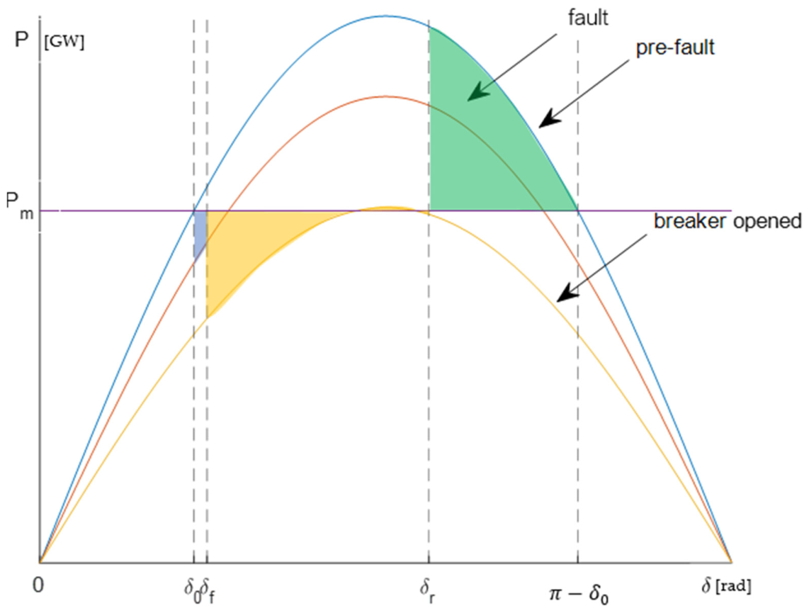
The maximum flow of power $p_0$ is determined by a single proper nonlinear equation obtained by imposing the equal area criterion in Equation (16) and graphically shown in Figure 2:

$${\int }_{{\delta }_0}^{{\delta (\Delta t}_{cl})}\left(p_0-{\displaystyle \frac{e_t^{\prime }e}{x_{totf}}}sen\delta \right)d\delta +{\int }_{{\delta (\Delta t}_{cl})}^{{\delta (\Delta t}_{cl}+{\Delta t}_r)}\left(p_0-{\displaystyle \frac{e_t^{\prime }e}{x_{totr}}}sen\delta \right)d\delta +{\int }_{{\delta (\Delta t}_{cl}+{\Delta t}_r)}^{{\pi -\delta }_0}\left(p_0-{\displaystyle \frac{e_t^{\prime }e}{x_{tot}}}sen\delta \right)d\delta =0$$

(16)

In Equation (16), it is not necessary, however, to integrate the last trajectory after reclosing since the final condition is set equal to the unstable equilibrium point ${\pi -\delta }_0$ with zero velocity. In addition, thanks to the integral formulation of the area criterion, it is enough to know the initial position, determined by Euler’s method as the final condition of the second trajectory, and the final position of this third segment of the trajectory, corresponding to the unstable equilibrium point.

The three integrals in Equation (16) can be expressed as function of the only unknown $p_0$ by keeping in mind the recursive form of the differential model:

$${\displaystyle \sum _{i=1}^{N_f}}\left(p_0-{\displaystyle \frac{e_t^{\prime }e}{x_{totf}}}sen(f_{f,2}^i\left(p_0\right))\right)h+{\displaystyle \sum _{i=1}^{N_r}}\left(p_0-{\displaystyle \frac{e_t^{\prime }e}{x_{totr}}}sen(f_{r,2}^i\left(p_0\right))\right)h+{\displaystyle \sum _{i=1}^{N_{pf}}}\left(p_0-{\displaystyle \frac{e_t^{\prime }e}{x_{totpf}}}sen(f_{pf,2}^i\left(p_0\right))\right)h=0$$

(17)

This nonlinear equation in the unknown $p_0$ can be efficiently solved by a numerical method.

Applying the Monte Carlo methodology, the TSM of power system under investigation is evaluated.

2.2. Formulation for Two Areas

In the Section 2.1, the problem of determining the stability margin with reference to the case of a single machine connected to an infinite power network was formulated. In this paragraph, based on what has been presented, the issue of determining the transient stability margin for two interconnected areas is addressed. It is of interest to examine how the stability margin depends on the inertia of the two areas, which will be subsequently described in terms of random variables.

First, it is appropriate to show how it is possible to reduce the problem of determining transient stability to the previous case, after defining the equivalent inertia of the two areas.

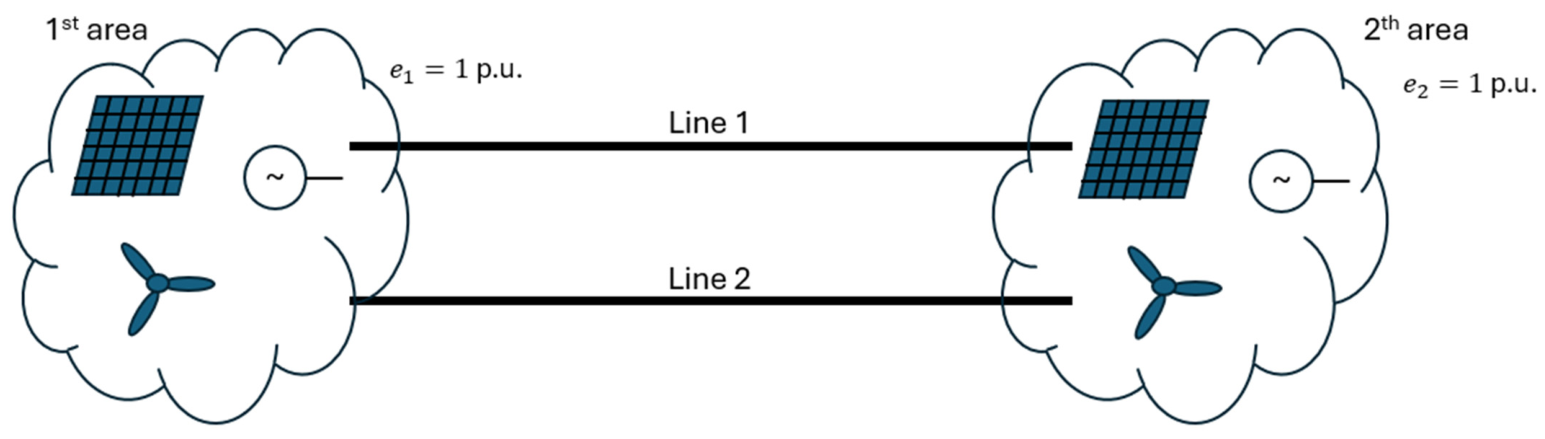
For this investigation the power system has been modelled considering two equivalent generators each delivering power through an equivalent transformer with its reactance $x_{tran1}$ and $x_{tran2}$ interconnected via double three-phase line: Figure 3. The two equivalent generators are assumed to have a constant voltage value ($e_1=e_2=1 \mathrm{p}.\mathrm{u}.$) and their direct transient and inverse sequence reactances $x_{d1}^{\prime }$, $x_{d2}^{\prime }$, $x_{i1}$ and $x_{i2}$ (the inverse transient reactances are assumed equal to subtransient reactances $x_{d1}^{″}$ and $x_{d2}^{″}$). As far as the double-three line is concerned, modeling is the one already examined previously.

Also in this case, the power transmitted between the two areas can be expressed according to a sinusoidal law depending on the rotor position, with a maximum amplitude dependent on a suitable equivalent reactance for the different phases of the transient.

For reasons of brevity of exposition, the expressions of the equivalent reactances are not reported, as they can be quickly obtained by borrowing what has already been done for the case of a single machine.

From an electromechanical point of view, the two-area system can be reduced to that of a single machine [18]. Considering the lossless system, the electromechanical dynamics are summarized by the system of two second-order differential equations:

$$\left\{\begin{array}{c}{\displaystyle \frac{d^2{\delta }_1}{dt}}={\displaystyle \frac{{\omega }_0}{T_{a1}}}\left(p_{m1}-{\displaystyle \frac{e_{t1}^{\prime }{e}_{t2}^{\prime }}{x_{eq}}}sen({\delta }_1-{\delta }_2)\right)\\ {\displaystyle \frac{d^2{\delta }_2}{dt}}={\displaystyle \frac{{\omega }_0}{T_{a2}}}\left(p_{m2}-{\displaystyle \frac{e_{t1}^{\prime }{e}_{t2}^{\prime }}{x_{eq}}}sen({\delta }_2-{\delta }_1)\right)\end{array}\right.$$

(18)

The electromechanical stability of the system depends on the difference in angular positions of the two rotors, so it is enough to subtract the second from the first of (18), obtaining:

$${\displaystyle \frac{d^2{(\delta }_1-{\delta }_2)}{dt}}={\displaystyle \frac{d^2{\delta }_{12}}{dt}}={\displaystyle \frac{{\omega }_0}{T_{a1}}}\left(p_{m1}-{\displaystyle \frac{e_{t1}^{\prime }{e}_{t2}^{\prime }}{x_{eq}}}sen({\delta }_1-{\delta }_2)\right)-{\displaystyle \frac{{\omega }_0}{T_{a2}}}\left(p_{m2}-{\displaystyle \frac{e_{t1}^{\prime }{e}_{t2}^{\prime }}{x_{eq}}}sen({\delta }_2-{\delta }_1)\right)$$

(19)

In the pre-fault conditions the following condition is assumed to be satisfied:

$$p_{m1}+p_{m2}=0$$

(20)

As a result, it can be written as

$${\displaystyle \frac{d^2{\delta }_{12}}{dt}}={\omega }_0\left({\displaystyle \frac{1}{T_{a1}}}+{\displaystyle \frac{1}{T_{a2}}}\right)\left(p_{m1}-{\displaystyle \frac{e_{t1}^{\prime }{e}_{t2}^{\prime }}{x_{eq}}}sen{\delta }_{12}\right)$$

(21)

One can then define the equivalent mechanical starting time which, borrowing the logic of electrical circuits, can be regarded as the parallel of the mechanical starting times of the individual areas:

$${\displaystyle \frac{d^2{\delta }_{12}}{dt}}={\displaystyle \frac{{\omega }_0}{T_{aeq}}}\left(p_{m1}-{\displaystyle \frac{e_{t1}^{\prime }{e}_{t2}^{\prime }}{x_{eq}}}sen{\delta }_{12}\right)$$

(22)

with $T_{a_{eq}}$:

$$T_{a_{eq}}={\displaystyle \frac{{T_a}_1{T_a}_2}{{T_a}_1{{+ T}_a}_2}}={\displaystyle \frac{1}{\frac{1}{{T_a}_1}+\frac{1}{{T_a}_2}}}$$

(23)

The primary aim of the paper is to critically evaluate the stability margin depending on the variability of the inertias of the two areas. Although, strictly speaking, the variability of the inertias should properly be addressed in terms of a stochastic process, in this context the issue will be tackled in terms of a static approach, specifically focusing attention on the correlation of the inertia of the two areas.

3. Probabilistic Characterization of Transient Stability as a Function of Areas Inertia

3.1. General Aspects of the Methodology

The interconnected electrical system is a dynamic system intrinsically characterized by randomness. Therefore, all quantities can be regarded, strictly speaking, as stochastic processes. It is more essential than ever to have tools that allow us to consider the impact of random factors, even by resorting to simplifying hypotheses.

First and foremost, according to what was discussed in the Section 2.1 of the present paper, it can be assumed that the quantities of interests are observed in each very “short time” interval due to rapid dynamic proprieties of fault event. This event interacts with the slower dynamic-related power system parameters such as random inertia value that, for this reason, may be assumed to be constant in time.

The fundamental characteristics of the probabilistic approach to the assessment of transient stability margins are first presented. This approach is necessary due to the stochasticity of the inertia of interconnected areas. However, inertia is not the only random variable; there can potentially be numerous. For example, it is enough to consider the fault type and location, the fault clearing phenomenon. In this paper, for sake of clarity and simplicity in addition to the inertias, the type of fault is considered a significant random variable, with any additional random variables being treated in the same way through the theorem of total probability.

Let $P\left(p_0\right)$ denote the cumulative probability function of the transient stability margin dependent on the randomness of inertia. For simplicity, let {E1, E2, E3, E4} be the set of fault types which constitute a set of credible and mutually exclusive contingencies.

The transient stability margin can then be calculated in the following way:

$$P\left(p_0\right)={\displaystyle \sum _{i=1}^4}P\left(p_0|E_i\right)P(E_i)$$

(24)

where

• $P\left(E_i\right)$ is the probability of occurrence of the fault $E_i$ over the time interval under consideration;
• $P\left(p_0|E_i\right)$ is the probability of the transient stability margin, once the fault $E_i$ occurs.

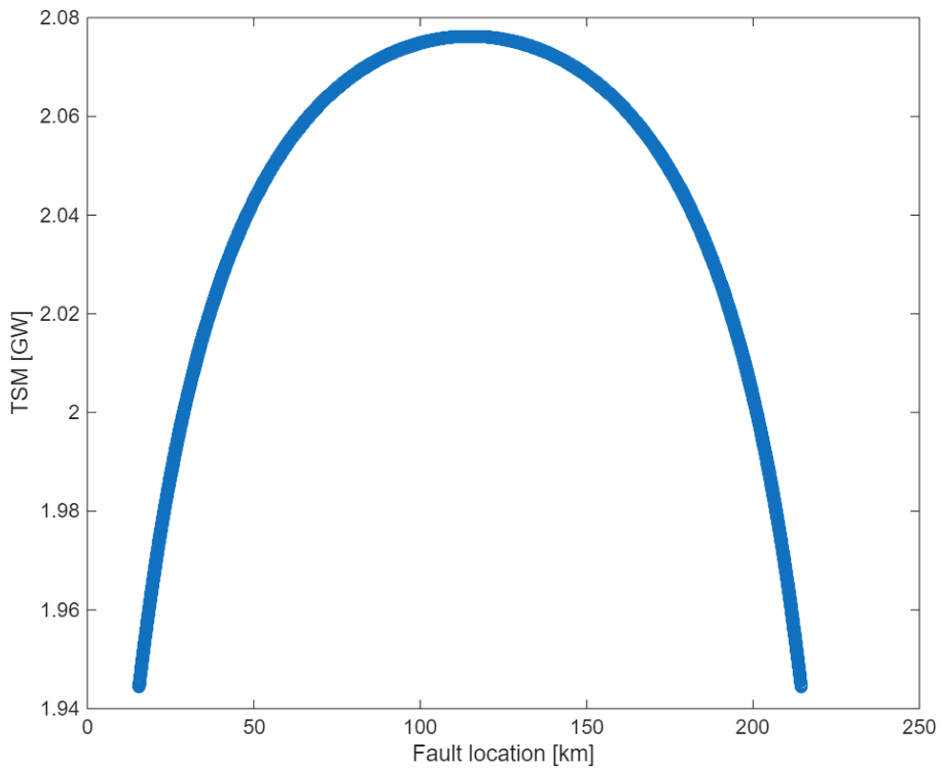
The fault statistics can be estimated based on past data relative to the power system under investigation and, therefore, $P\left(E_i\right)$ can be considered quantities that are very reasonably well known. In the same way as the type of fault, the randomness of the fault location could be treated obtaining results as those shown in Figure 4 for single-phase line-to-ground fault. For example, in this analysis, it was assumed that the occurrence of a fault in any of the small portions into which the central section of the double three-phase line connecting two areas of an electrical network was divided is equiprobable. In this case, the results show that faults occurring near one of two areas are those that most significantly limit TSM.

So, what constitutes the core of the issue addressed by the paper is the evaluation of $P\left(p_0|E_i\right)$. In the literature, there exists a plurality of probabilistic methodologies. The paper focuses attention on the classic linearized probabilistic method and on the Monte Carlo method. The aim of the paper, in fact, is not to find the best method but rather to provide useful tools both in the planning phase and in the operation of the electrical system, intended to support decisions in a flexible and rational way.

Based on a preliminary sensitivity analysis reported in Section 3.2, it will be shown that the linearized probabilistic approach appears as a legitimate candidate to be used. However, it could turn out to be not very accurate in the tails of the distribution and, therefore, it could be inadequate for some aspects related to free market logic. In such a case, the robust Monte Carlo method seems to be the simplest and most appropriate method for the rapid determination of the distributional properties of the transient stability margin.

3.2. Sensitivity Analysis of Stability Margins

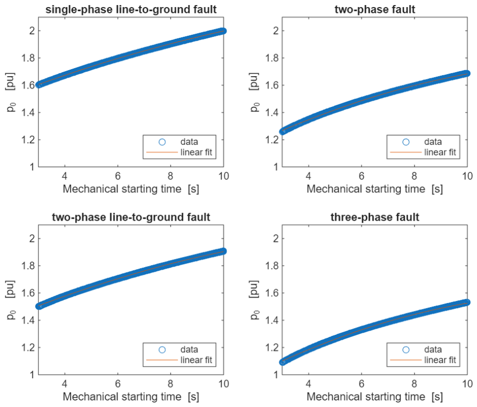
From numerous simulations carried out on a two-area system, it was observed that the stability margin is an increasing function of the equivalent inertia, following an almost linear law. In Figure 5, the stability margin curves are shown for the four types of faults considered, namely three-phase fault, line-to-ground double-phase fault, two-phase fault, and single-phase line-to-ground fault for the two-area system whose data are reported in the numerical application.

The equivalent inertia is assumed to vary in the range 3 to 10 s considering 701 samples. As can be seen, for all types of faults, it can be stated that the linear variation law can be considered satisfied with a truly satisfactory approximation, above all for single-phase line-to-ground fault. Indeed, the linearization error relative to the TSM values obtained from the previously described methodology has a very low mean value, equal to approximately $7.7\times {10}^{-4}$ p.u. Although at the tails (around inertia values of 3 s and 10 s) the approximation is less accurate (this will be discussed later), the 95th percentile of error is about of $1.6\times {10}^{-4}$ p.u. For the other types of faults, the accuracy is slightly lower, but still sufficient for the physical evaluation of the obtained values (see

Table 2. TSM as a function of inertia linearization error for the various fault typologies.

Earth Fault Type	Error Mean Value [p.u.]	95th Percentile of Error [p.u.]
Single-phase	$7.7\times {10}^{-4}$	$1.6\times {10}^{-3}$
Two-phase	$2.2\times {10}^{-3}$	$4.7\times {10}^{-3}$
Two-phase ground	$1.3\times {10}^{-3}$	$2.7\times {10}^{-3}$
Three-phase	$2.6\times {10}^{-3}$	$5.5\times {10}^{-3}$

).

Consequently, since transient stability margin $p_0$ for each type of fault depends linearly on the equivalent mechanical starting time $T_{a_{eq}}$, it can be optimally approximated by a linear law of the type

$$p_0=a+b{T}_{a_{eq}}$$

(25)

in which parameters $a$ and $b$ are obtained from linearization.

In Section 4 the approximation is justified by proof theoretical and numerical analysis.

3.3. Transient Stability and Areas Inertia Correlation

In a static approach of probability, which is certainly appropriate for us from a planning perspective and for forecasting stability properties, the randomness of the inertia of the various areas can be described in terms of multivariate distribution. In particular, the primary objective of this paper is to evaluate the stability margins as function of the correlation of these random variables. To achieve this objective, it is first necessary to assess the impact of the correlation between random variables of inertia of the two areas ${T_a}_1$ and ${T_a}_2$ on the $T_{a_{eq}}$.

Now, to demonstrate the generality of the methodology, two multivariate distributions are employed. The first relates to the characterization of inertia as a lognormal random variable: the lognormal model is one of the most popular in applied probability and this characterization is also in line with what some of the authors have already proposed in previous scientific papers [11]. The second multivariate distribution is related to the gamma distribution, which was chosen for its flexibility, in a certain way, to approximate distributions related to available real data. In this paper, based on what was presented in [20], a suitable optimization problem is formulated for generating samples distributed according to the multivariate gamma distribution.

3.3.1. Multivariate Lognormal Random Inertia

As described above, the randomness of inertia of various areas of a power system can be modelled with a multivariate lognormal probability density of the inertia variables $\mathit{y}={\mathrm{e}}^{\mathit{x}}$, with $\mathit{x}=\left[\begin{array}{c}\begin{array}{c}{X}_1\\ X_2\end{array}\\ \begin{array}{c}\cdots \\ X_n\end{array}\end{array}\right]$ vector of $n$ normal distribution variables with the probability density function

$$f_{\mathit{x}}\left(\mathit{x}\right)={\displaystyle \frac{1}{\sqrt{{\left(2\pi \right)}^n\left|\mathsf{\Sigma }\right|}}}{\mathrm{e}}^{-{\displaystyle \frac{1}{2}}{\left(\mathit{x}-\mathit{\mu }\right)}^{\prime }{\mathsf{\Sigma }}^{-1}\left(\mathit{x}-\mathit{\mu }\right)}$$

(26)

where $\mathit{\mu }$ and $\mathsf{\Sigma }$ are the vector of means and the $n\times n$ variance matrix.

For the investigation of this work in which the TSM is evaluated in a power system characterized by two areas interconnected with a double three-phase line, weakly interacting, the inertias PDF of two areas can be assumed as two variables $\mathit{y}=\left[\begin{array}{c}{y}_1\\ y_2\end{array}\right]=\left[\begin{array}{c}{\mathrm{e}}^{{\mathit{X}}_{\mathbf{1}}}\\ {\mathrm{e}}^{{\mathit{X}}_{\mathbf{2}}}\end{array}\right]$ with a variable correlation coefficient ${\rho }_{1,2}$. Starting from mean $\mathbb{E}\left[\mathit{y}\right]=\left[\begin{array}{c}\mathbb{E}\left[y_1\right]\\ \mathbb{E}\left[y_2\right]\end{array}\right]$, variances matrix

$${\mathsf{\Sigma }}_{\mathit{y}}=\left[\begin{array}{cc}{{\sigma }_{y_1}}^2\hfill & \hfill {\rho }_{1,2}{\sigma }_{y_1}{\sigma }_{y_2}\\ {\rho }_{1,2}{\sigma }_{y_1}{\sigma }_{y_2}\hfill & \hfill {{\sigma }_{y_2}}^2\end{array}\right],$$

(27)

with standard deviations ${\sigma }_{y_1}$ and ${\sigma }_{y_2}$ of two variables $\left[\begin{array}{c}{y}_1\\ y_2\end{array}\right]$, the mean $\mathit{\mu }$ and variance matrix $\mathsf{\Sigma }$ of the multivariate lognormal probability density is obtained from following relationships:

$$\mathbb{E}\left[\mathit{y}\right]={\mathrm{e}}^{\mathit{\mu }+\mathsf{\Sigma }/\mathbf{2}}\Rightarrow \mathit{\mu }=\mathrm{d}\mathrm{i}\mathrm{a}\mathrm{g}\left(\mathrm{l}\mathrm{n}\left(\mathrm{d}\mathrm{i}\mathrm{a}\mathrm{g}\left(\mathbb{E}\left[\mathit{y}\right]\right)\right)\right)-\mathrm{d}\mathrm{i}\mathrm{a}\mathrm{g}\left(\mathsf{\Sigma }/\mathbf{2}\right)$$

(28)

$${\mathsf{\Sigma }}_{\mathit{y}}=\mathrm{d}\mathrm{i}\mathrm{a}\mathrm{g}\left(\mathbb{E}\left[\mathit{y}\right]\right)\left({\mathrm{e}}^{\mathsf{\Sigma }}-1_{n\times n}\right)\mathrm{d}\mathrm{i}\mathrm{a}\mathrm{g}\left(\mathbb{E}\left[\mathit{y}\right]\right)\Rightarrow \mathsf{\Sigma }=\mathrm{l}\mathrm{n}\left(1_{n\times n}+{\mathrm{d}\mathrm{i}\mathrm{a}\mathrm{g}\left(\mathbb{E}\left[\mathit{y}\right]\right)}^{-1}{\mathsf{\Sigma }}_{\mathit{y}}{\mathrm{d}\mathrm{i}\mathrm{a}\mathrm{g}\left(\mathbb{E}\left[\mathit{y}\right]\right)}^{-1}\right)$$

(29)

In this manner it is possible to obtain the probability density in (28) useful for TSM evaluation for the two-area power system with correlated inertia.

3.3.2. Multivariate Gamma Distribution

While the multivariate lognormal distribution was obtained with a closed-form solution, the multivariate gamma distribution is obtained from the statistical parameters of the individual variables by an optimization procedure. Considering a multivariate gamma as the joint distribution of linear combination,

$$Z_i={\displaystyle \frac{{\beta }_i}{{\beta }_0}}{V}_o\left({\alpha }_0,{\beta }_0,{\gamma }_0\right)+V_i\left({\alpha }_i,{\beta }_i,{\gamma }_i\right),$$

(30)

of independent gamma variables $V_i$ (as in [20]), each with a density

$$f_{v_i}\left(v_i;{\alpha }_i, {\beta }_i,{\gamma }_i\right)={\displaystyle \frac{{\left(v_i-{\gamma }_i\right)}^{{\alpha }_i-1}}{{{\mathsf{\beta }}_i}^{{\alpha }_i}\Gamma \left({\alpha }_i\right)}}{\mathrm{e}}^{-\left(v_i-{\gamma }_i\right)/{\beta }_i},$$

(31)

in which $v_i>{\gamma }_i$, ${\alpha }_i>0$, ${\beta }_i>0$ and $i\le n$, where $n$ is the gamma variables number; this procedure is based on a minimization of the module of the $x=\left[\alpha \left(1:n\right) \beta \left(1:n\right) \gamma \left(1:n\right) {\alpha }_0 {\beta }_0 {\gamma }_0\right]$ vector of gamma distribution parameters (shape, scale and location parameters for each variable, respectively), assuming $\alpha \left(1:n\right)$, $\beta \left(1:n\right)$, ${\alpha }_0$ and ${\beta }_0$ strictly positive, and applying the following constraints:

$$\mathbb{E}\left[Z_i\right]=\left({\alpha }_0+{\alpha }_i\right){\beta }_i+\left({\gamma }_0/{\beta }_0\right){\beta }_i+{\gamma }_i,$$

(32)

$${{\sigma }_{Z_i}}^2=\left({\alpha }_0+{\alpha }_i\right){{\beta }_i}^2 \mathrm{and}$$

(33)

$$Cov\left[Z_i,Z_j\right]={\alpha }_0{\beta }_i{\beta }_j, \mathrm{for} i\ne j$$

(34)

for obtaining $x$ vector and then evaluating gamma variables $V_o$ and $Z_i$.

3.3.3. Sensitivity Analysis of Equivalent Inertia

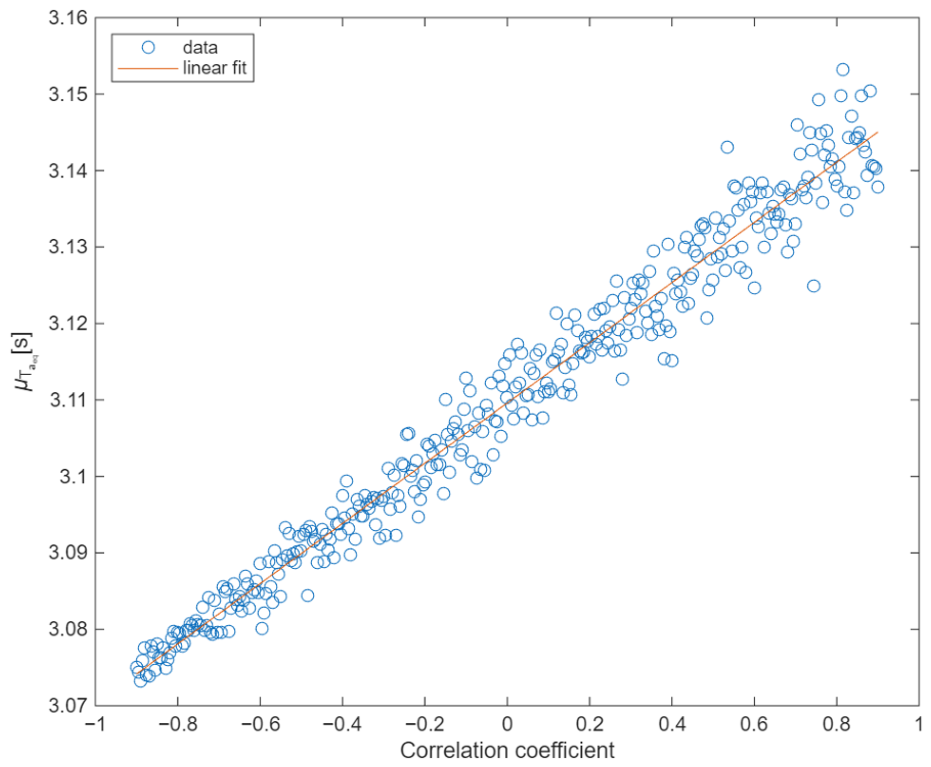
Considering a power system consisting of two areas whose inertias ${T_a}_1$ and ${{ T}_a}_2$ are correlated, we examine the influence of this correlation on the mean value of equivalent inertia ${\mu }_{T_{a_{eq}}}=\mathbb{E}\left[T_{a_{eq}}\right]$ of the entire power system, evaluated according to Equation (23), assuming, for brevity, only the case in which the inertias of the two areas are described by multivariate lognormal random variables. The same considerations can also be made for other possible probability densities, such as the multivariate gamma distribution analyzed in this paper.

Figure 6 shows the relationship between the mean value of the equivalent inertia and the correlation of the inertias of the two areas of the power system. As can be seen, a linearization can be applied, obtaining an error with a low mean value equal to approximately $6\times {10}^{-7} \mathrm{s}$ and the 95th percentile of error about 0.0055 s.

Then, $\mathbb{E}\left[T_{a_{eq}}\right]$ has been found to numerically depend linearly on the correlation coefficient $\rho$ of the inertias of the two areas:

$$\mathbb{E}\left[{T_a}_{eq}\right]=c+d\rho$$

(35)

where the parameters $c$ and $d$ were obtained from linearization. From Equations (25) and (35), it is possible to characterize the stability margin mean value $\mathbb{E}\left[p_0\right]$ as a function of the correlation of area moments of inertia, thereby deriving the linearized method:

$$\mathbb{E}\left[p_0\right]=a+b\left(c+d\rho \right)=\left(a+bc\right)+bd\rho$$

(36)

For a single-phase fault the linearization error mean value corresponds to 0.02 GW on an expected TSM value of about 1.61 GW and the 95th percentile value is 0.0246 GW: considering this latter value, the error amounts to about 1.5% of the expected values.

4. Impact of Inertia on Stability Margins

In pre-fault stationary conditions, the phase angle $\delta$ of equivalent synchronous machines of OMIB of the power system area is constant, while, in presence of a fault, the stationary condition of operational status of power system area is loss and $\delta$ parameter is affected by an accelerating or decelerating force according with the swing equation in Equation (11). Since the typical fault clearance times $∆t_{cl}$ and the circuit breaker reclosing times $∆t_r$ are very quick, around values of 0.1 s and 0.3 s, respectively, the accelerated/decelerated angular motion obtained can be assumed uniformly accelerated/decelerated for each different time slot. In the first approximation, the TSM can be assumed with a linear dependence on the angular phase value of the equivalent synchronous generator.

During fault clearance time the phase angle motion $\delta \left(t\right)$, starting from a stationary condition ($\omega ={\omega }_0$) with $\delta =const$ and phase angle speed $v_{\delta }\left(0\right)={\left.{\displaystyle \frac{d\delta }{dt}}\right|}_{t=0}=0$, becomes

$$\delta \left(t\right)={\delta }_0+{\displaystyle \frac{1}{2}}{a}_f{t}^2$$

(37)

with

$$a_f={\displaystyle \frac{d^2\delta }{{dt}^2}}\cong {\left.{\displaystyle \frac{d^2\delta }{{dt}^2}}\right|}_{t=∆t_f}={\displaystyle \frac{{\omega }_0}{T_a}}\left(p_m-{p_e}_f\left({{\delta }_f}^{-}\right)\right)=const$$

(38)

obtaining

$${\delta }_f\cong {\delta }_0+{\displaystyle \frac{1}{2}}{\displaystyle \frac{{\omega }_0}{T_a}}\left(p_m-{p_e}_f\left({{\delta }_f}^{-}\right)\right){∆t_f}^2$$

(39)

where ${p_e}_f\left({{\delta }_f}^{-}\right)$ is active electric power at the end of fault clearance time interval ($\delta \left(∆t_{cl}\right)={\delta }_f$ as indicated in Figure 2).

In Equation (38) the values ${\delta }_f$ depend on ${\displaystyle \frac{1}{T_a}}$. For the typical values around 6 s and variability range of $T_a$ of ±3 s (in two following equations $T_a$ defined value is labelled as $\widetilde{T_a}$) the expression can be expanded on base of Taylor series obtaining a linear dependence of phase angles value ${\delta }_f$:

$${\displaystyle \frac{1}{T_a}}\cong {\displaystyle \frac{1}{\widetilde{T_a}}}-{\displaystyle \frac{1}{{\widetilde{T_a}}^2}}\left(T_a-\widetilde{T_a}\right)$$

(40)

and

$${\delta }_f\cong {\delta }_0+{\displaystyle \frac{1}{2}}{\omega }_0\left(p_m-{p_e}_f\left({{\delta }_f}^{-}\right)\right){∆t_f}^2\left[{\displaystyle \frac{1}{\widetilde{T_a}}}-{\displaystyle \frac{1}{{\widetilde{T_a}}^2}}\left(T_a-\widetilde{T_a}\right)\right]$$

(41)

The same analysis can also be extended to other time intervals in the sequence of different configurations of the electrical system that occur following a fault. Therefore, the theoretical evaluation of the variability of the phase angle ${\delta }_f$ as a function of the equivalent inertia of the electrical system reported in Equation (40) can be extended to the other phase angles ${\delta }_0$ and ${\delta }_r=\delta \left(∆t_{cl}+{ ∆t}_r\right)$ and can be supported by the Monte Carlo methodology.

In fact, starting from a possible probability distribution of the random variable of the inertia of the electrical system defined on the basis of typical values that this parameter can assume in an actual network, with the Monte Carlo methodology it is possible to validate the observations on the linearity of the various parameters during the various phases of a fault by analyzing the variability of their distribution through the coefficients of variation ${CV}_k$ in Equation (41) and the Pearson coefficient in Equation (42) evaluated in correlation with the inertia variable (with the index $k$ indicating one of various fault process parameters):

$${CV}_k={\displaystyle \frac{{\sigma }_k}{\mathbb{E}\left[k\right]}},$$

(42)

$$r_{k,T_a}={\displaystyle \frac{Cov\left[T_a,k\right]}{{\sigma }_{T_a}{\sigma }_k}}$$

(43)

where $\mathbb{E}\left[·\right]$ ${\sigma }_{·}$ are the mean and standard deviation operators.

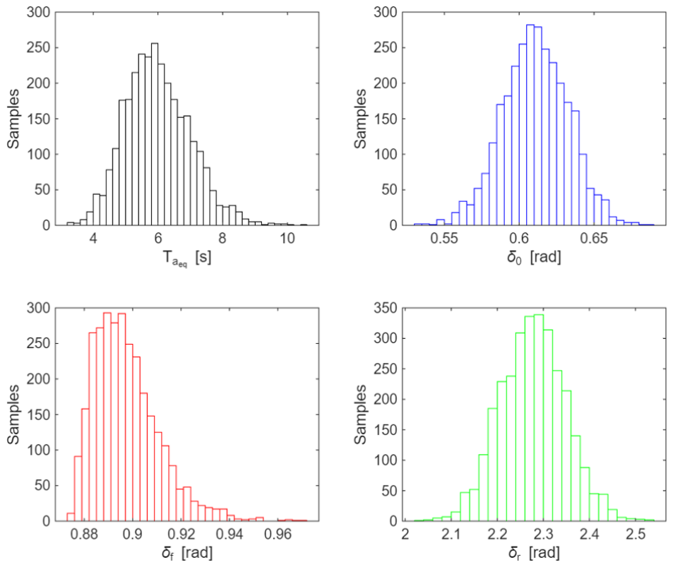
The results obtained for fault types reported in Table 1, assuming a realistic lognormal probability distribution of the power system with an equivalent inertia $T_{a_{eq}}$ (power system consisting of two areas, see Section 2.2) between 3 s and 10 s (distribution shown at the top left in Figure 7) are reported in

Table 3. Lognormal probability variables parameters for different fault types.

Earth Fault Type	$\mathit{k}$	$\mathbb{E}\left[\mathit{k}\right]$	${\mathit{\sigma }}_{\mathit{k}}$	${\mathit{C}\mathit{V}}_{\mathit{k}}$ [%]	${\mathit{r}}_{\mathit{k},{\mathit{T}}_{\mathit{a}}}$
	${\mathit{T}}_{\mathit{a}}$	6 s	1 s	16.7	1
Three-phase	${\delta }_0$	0.61 rad	0.022 rad	3.6	0.9937
	${\delta }_f$	0.90 rad	0.013 rad	1.5	−0.9405
	${\delta }_r$	2.28 rad	0.070 rad	3.1	−0.9939
	$A_f$	0.38 GW rad	0.028 GW rad	7.5	−0.9867
	$A_r$	−0.32 GW rad	0.049 GW rad	15.3	0.9957
	$A_m$	−0.06 GW rad	0.021 GW rad	35.5	−0.9998
	TSM	1.33 GW	0.062 GW	4.6	0.9959
Single-phase	${\delta }_0$	0.77 rad	0.015 rad	2.0	0.9979
	${\delta }_f$	0.92 rad	0.005 rad	0.6	−0.7737
	${\delta }_r$	2.00 rad	0.053 rad	2.7	−0.9954
	$A_f$	0.10 GW rad	0.008 GW rad	7.9	−0.9843
	$A_r$	0.01 GW rad	0.028 GW rad	227.1	0.9954
	$A_m$	−0.11 GW rad	0.020 GW rad	19.0	−0.9978
	TSM	1.83 GW	0.056 GW	3.1	0.9991
	${\delta }_0$	0.66 rad	0.020 rad	2.9	0.9943
	${\delta }_f$	0.91 rad	0.011 rad	1.2	−0.9196
Two-phase	${\delta }_r$	2.19 rad	0.064 rad	2.9	−0.9938
	$A_f$	0.27 GW rad	0.021 GW rad	7.7	−0.9844
	$A_r$	−0.20 GW rad	0.042 GW rad	−20.8	0.9949
	$A_m$	−0.07 GW rad	0.021 GW rad	−29.3	−0.9995
	TSM	1.48 GW	0.060 GW	4.0	0.9965
Two-phase ground faults	${\delta }_0$	0.73 rad	0.017 rad	2.3	0.9964
	${\delta }_f$	0.92 rad	0.008 rad	0.9	−0.8677
	${\delta }_r$	2.08 rad	0.057 rad	2.7	−0.9945
	$A_f$	0.15 GW rad	0.012 GW rad	7.9	−0.9832
	$A_r$	−0.06 GW rad	0.033 GW rad	−56.0	0.9948
	$A_m$	−0.09 GW rad	0.021 GW rad	−22.4	−0.9984
	TSM	1.70 GW	0.06 GW	3.4	0.9981

.

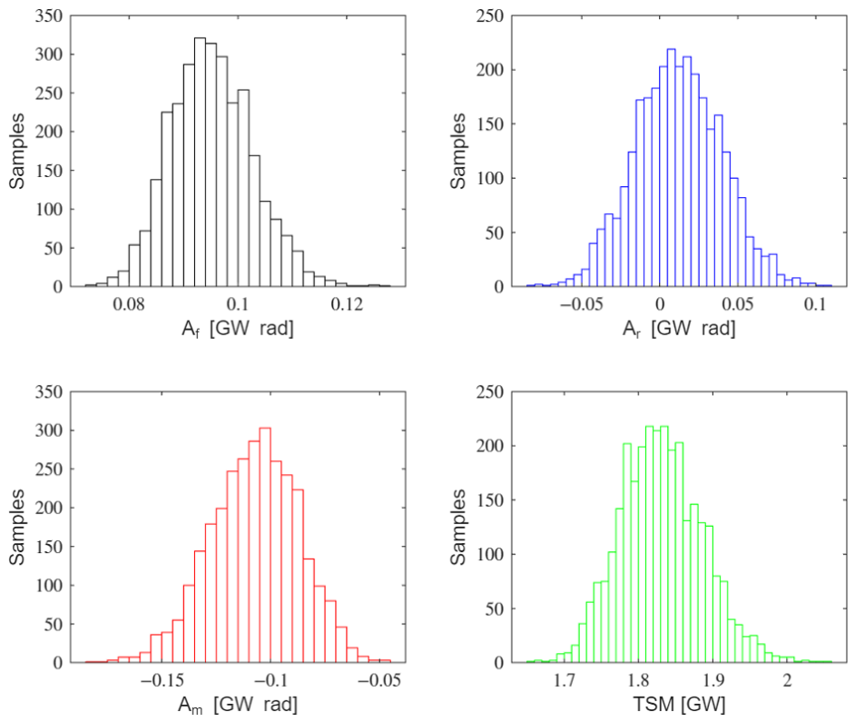
Some cases for three-phase and single-phase faults are described in detail as examples. For the three-phase fault, the distributions of the random variables of the phase angles (${\delta }_0$, ${\delta }_f$, ${\delta }_r$) of the equivalent synchronous machine are shown in Figure 7 at the top right and in the two graphs at the bottom left and right, respectively. As can be seen in Figure 7 and Table 3, the coefficients of variation (${CV}_{{\delta }_0}$, ${CV}_{{\delta }_f}$, ${CV}_{{\delta }_r}$) of angular phases (${\delta }_0$, ${\delta }_f$, ${\delta }_r$) are very low, especially for ${\delta }_f$, demonstrating the very slight variation in angular phases as a function of the different inertia values.

For this reason, the approximation in Equation (40) can be confirmed without losing its validity. This is even more valid for the case of single-phase-to-ground fault, as reported in Table 3.

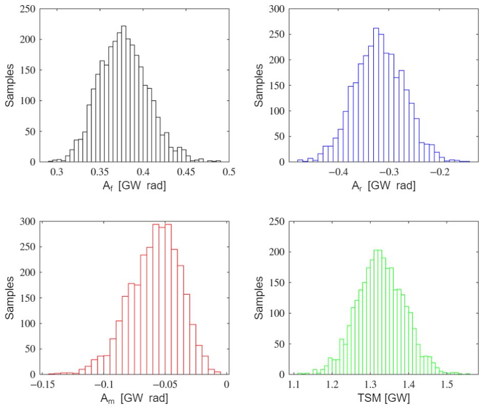
The linear dependence can also be associated with the areas defined in Figure 2 and shown in Figure 8 and Figure 9 for three-phase and single-phase ground faults, respectively. These areas represent the increase (positive values) or decrease (negative values) in the kinetic energy of the equivalent rotating synchronous machine for the different power supply system configurations during the fault process.

The two graphs at the top left and right, and at the bottom left of Figure 8 show the distributions of the different areas $A_f$, $A_r$ and $A_m$ defined in Figure 2, delimited by the phase angles ${\delta }_0$ and ${\delta }_f$, ${\delta }_f$ and ${\delta }_r$, and ${\delta }_r$ and $\pi -{\delta }_0,$ respectively. During the reclosing and post-reclosing times, the negative values of the areas represent a deceleration of the equivalent synchronous machine that compensates for the positive acceleration area during the fault elimination time.

The same considerations could be made considering the acceleration and deceleration areas in Figure 9 relating to the single-phase fault (the numerical characteristics are shown in Table 3).

In this case, the reclosing area can take on negative or positive values as the equivalent inertia of the power system varies, while $A_f$ and $A_m$ maintain their acceleration (positive values) and deceleration (negative values) characteristics as in the case of the three-phase ground fault. For this reason, ${CV}_{A_r}$ assumes an anomalous (very high) value, unrelated to an actual high variation in the occurrences of the $A_r$ distribution.

Moreover, the Pearson correlation coefficients $r_{k,T_a}$ reported in Table 3 highlight the linear dependence of all parameters on the equivalent inertia of the power system.

The linear dependence on the equivalent inertia of the power system is confirmed above all for the random variable TSM obtained with the methodology adopted in this article for both three-phase and single-phase ground faults. The probability distributions of these variables are shown respectively at the bottom right in Figure 8 and Figure 9 and described numerically in Table 3. The Pearson correlation coefficients $r_{k,T_a}$ reported in Table 3 highlight the linear dependence of all parameters on the equivalent inertia of the power system. The investigation conducted gives information also on impact of inertia different values on the TSM random variables.

In particular, the TSM random variable associated with the double three-phase line of the power system under consideration assumes a mean value of 1.33 GW in the case of a three-phase ground fault, while it reaches a mean value of 1.83 GW in the case of a single-phase ground fault. Considering the 2% and 98% percentiles of the random variables examined, it is possible to identify the impact of the variation in inertia on the TSM:

-

An inertia interval between 4.23 and 8.49 s corresponds to a TSM variability between 1.72 and 1.97 GW for a three-phase fault (dependence with a linear coefficient of approximately 58.7 MW/s);

-

An inertia interval between 4.23 and 8.3 s corresponds to a TSM variability between 1.21 and 1.46 GW for a single-phase ground fault (dependence with a linear coefficient of approximately 61.4 MW/s).

These data show a greater impact of the variability of the system inertia on the TSM for the three-phase ground fault (and two-phase ground faults, see Table 3) than in the case of the single-phase fault (and two-phase faults, see Table 3), for which, on the other hand, a greater capacity for the line was assessed in terms of TSM.

5. Numerical Results

In the presence of a power grid assumable as constituted of two areas, weakly connected through a double three-phase line of 230 km, the transient stability margin, obtained considering a single-phase ground fault, can be evaluated modeling the inertia contribution of each area as provided from an equivalent synchronous machine. Each of these two equivalent synchronous machines will be characterized by an inertia value corresponding to total contribution of each different actual generator in the area. These generators could be traditional generators (synchronous machines with their high inertia values) and renewable generators with their typically low and non-programmable inertia values. The interaction between these generator types in each area makes the probabilistic modelling of inertia necessary to a comprehensive analysis of transient stability of the transmission network. For this reason, the probability density function of inertia of each area (${T_a}_1$ and ${T_a}_2$) has been assumed to be that of lognormal variables or gamma variables. Here, to illustrate different cases which can occur in practice, three cases are considered, and in each one of them it is assumed that ${T_a}_1$ and ${T_a}_2$ follow a LN PDF or gamma PDF:

• Case A—Independent inertias, with equal means;
• Case B—Independent inertias, with different means;
• Case C—Not independent inertias (not null correlation between ${T_a}_1$ and ${T_a}_2$ PDFs).

As described previously, TSM is evaluated through a Monte Carlo technique. For this investigation in each simulation 10,000 samples have been considered and convergence occurs generally after about 100 s (value in according with that obtained in the simulation reported in Section 3.2 in which, considering 701 samples, a simulation time of about of 7 s is obtained) when at least one of two convergence criteria (44), with ${\in }_{step}={10}^{-10}$, and first-order optimality of Karush–Kuhn–Tucker (KKT) condition [21] with a tolerance of ${10}^{-19}$ is satisfied:

$$\left|p_0\left(j\right)-p_0\left(j-1\right)\right|\le {\in }_{step}\ast \left(1+\left|p_0\left(j\right)\right|\right)$$

(44)

where $j$ index represents the order number of iteration for which the convergence criterion has been checked. For each sample a simulation time of about 0.01 s occurs. These simulation times obtained with a commercial notebook are acceptable for planning and operation studies of power systems. For online/real-time investigation, an improvement in the simulation architecture is needed.

The results presented in this section demonstrate undeniable usefulness both in the planning phase and in the operation of electrical systems. In the framework of progressive penetration of renewable sources into the generation portfolio, ensuring the transmission system is adequate to allow increases in power transfer between areas while respecting safe operating limits and determining stability margins in the face of credible contingencies become necessary elements for supporting the decisions of the network operator. The calculation of these margins can be decisive in establishing production access priorities within the logic of the free market. An improper assessment could be subject to disputes, even with significant economic consequences.

5.1. Case A—Independent Inertias, with Equal Means

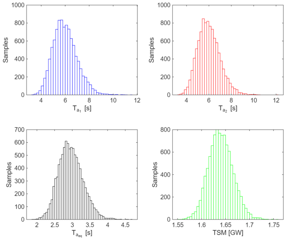
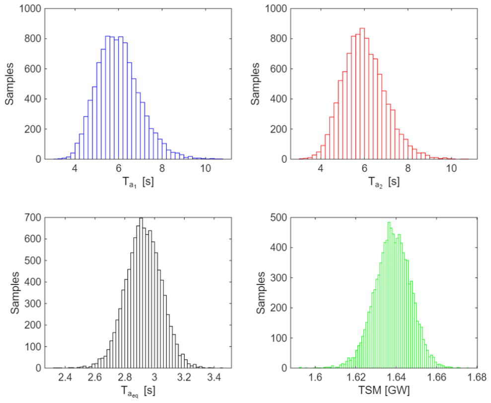
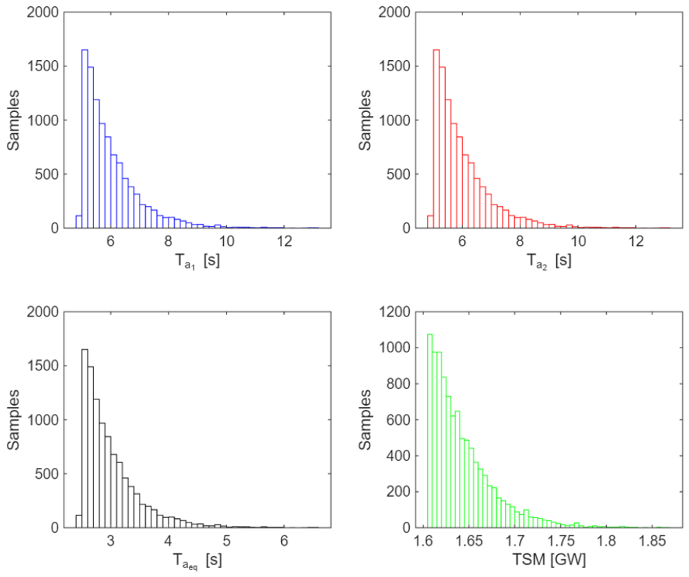
For this case, we assume for each area an equivalent probabilistic inertia lognormal variable with a typical mean value $\mathbb{E}\left[{T_a}_1\right]= \mathbb{E}\left[{T_a}_2\right]=6$ s and a standard deviation ${\sigma }_{{T_a}_1}={\sigma }_{{T_a}_2}=1$ s corresponding to a 16.7% with respect to its mean values. Figure 10 shows the equivalent inertia PDFs of each of two areas (at the top), the PDF resulting from the interaction between two areas (at the bottom in the left side) and the TSM PDF for the line connecting the two areas (at the bottom in the right side).

The total equivalent inertia PDF is characterized by a mean value of about $\mathbb{E}\left[T_{a_{eq}}\right]=2.96 \mathrm{s}$ and a ${\sigma }_{T_{a_{eq}}}\cong 0.34 \mathrm{s}$. Indeed, the total inertia $T_{a_{eq}}$ has a mean value which can be roughly approximated as follows:

$$\mathbb{E}\left[{T_a}_{eq}\right]=\mathbb{E}\left[{T_a}_1{T_a}_2/\left({T_a}_1+{T_a}_2\right)\right]\approx \mathbb{E}\left[{T_a}_1\right]E\left[{T_a}_2\right]/\mathbb{E}\left[{T_a}_1+{T_a}_2\right]=3 \mathrm{s}.$$

(45)

Such approximation is rather satisfactory, but it is shown here only to get an idea on the order of magnitude of $T_{a_{eq}}$. On the other hand, the evaluated TSM PDF (Figure 10 at bottom in right side) can be fit with a lognormal variable and assumes the mean value of 1.64 GW and a standard deviation of about 25.2 MW. The TSM developed, starting from the lognormal inertia variable, keeps the lognormal distribution for TSM. This is due to its almost linear dependence from inertia on the typical parameter values of real electrical systems as discussed in Section 3.

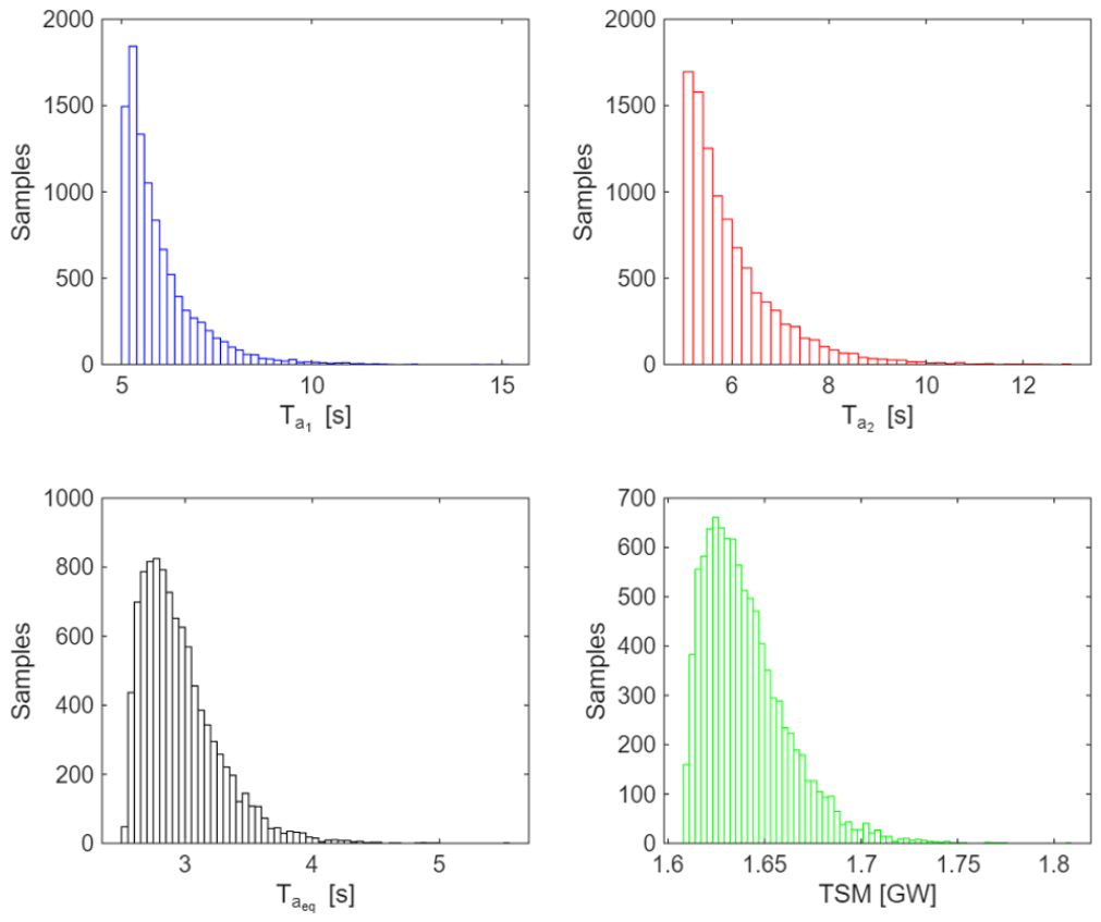
Analogous results can be obtained by assuming a gamma PDF for the variables ${T_a}_1$ and ${T_a}_2$ as visible in Figure 11.

Indeed, also in this case a mean value of about $\mathbb{E}\left[T_{a_{eq}}\right]\cong 2.96 \mathrm{s}$ and a standard deviation ${\sigma }_{{T_a}_{eq}}\cong 0.31 \mathrm{s}$ occurs. In each case the PDF of total inertia of a power system consisting in the areas weakly connected and uncorrelated is meanly reduced with respect to the inertia of each single area. Applying the methodology investigated for TSM evaluation, the margin values obtained are characterized by a PDF with mean value of 1.64 GW and a standard deviation of 22 MW.

5.2. Case B—Independent Inertias, with Different Means

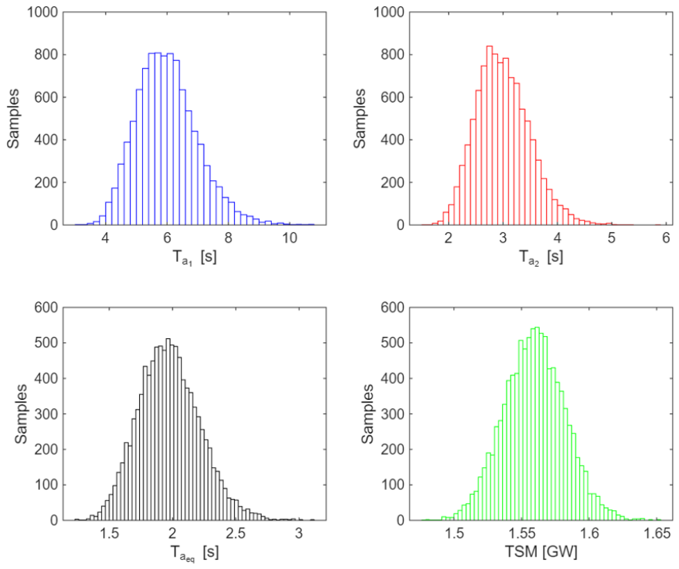
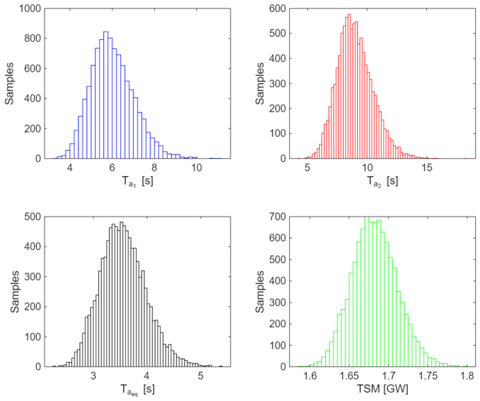
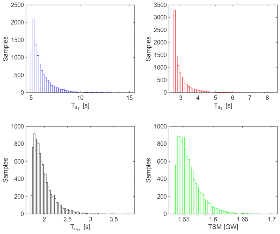
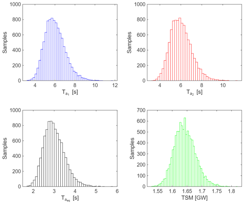
In this case the influence of different mean values of inertia for two areas on TSM is investigated. Given a fixed inertia PDF mean value for the first area ($\mathbb{E}\left[{T_a}_1\right]=6 \mathrm{s}$), the inertia PDF mean value for the second area ranges between 3 s and 9 s (typical range of variation in inertia) assuming a standard deviation of 16.7% of related mean value. For the inertia PDF mean value of the second area equal to $\mathbb{E}\left[{T_a}_2\right]=3 \mathrm{s}$ and interacting with inertia of the first areas, the total equivalent inertia PDF is characterized by $\mathbb{E}\left[T_{a_{eq}}\right]=1.98 \mathrm{s}$ and a ${\sigma }_{{T_a}_{eq}}\cong 0.24 \mathrm{s}$. The TSM obtained is characterized by a PDF with mean value of 1.56 GW and a standard deviation of 22.7 MW (Figure 12).

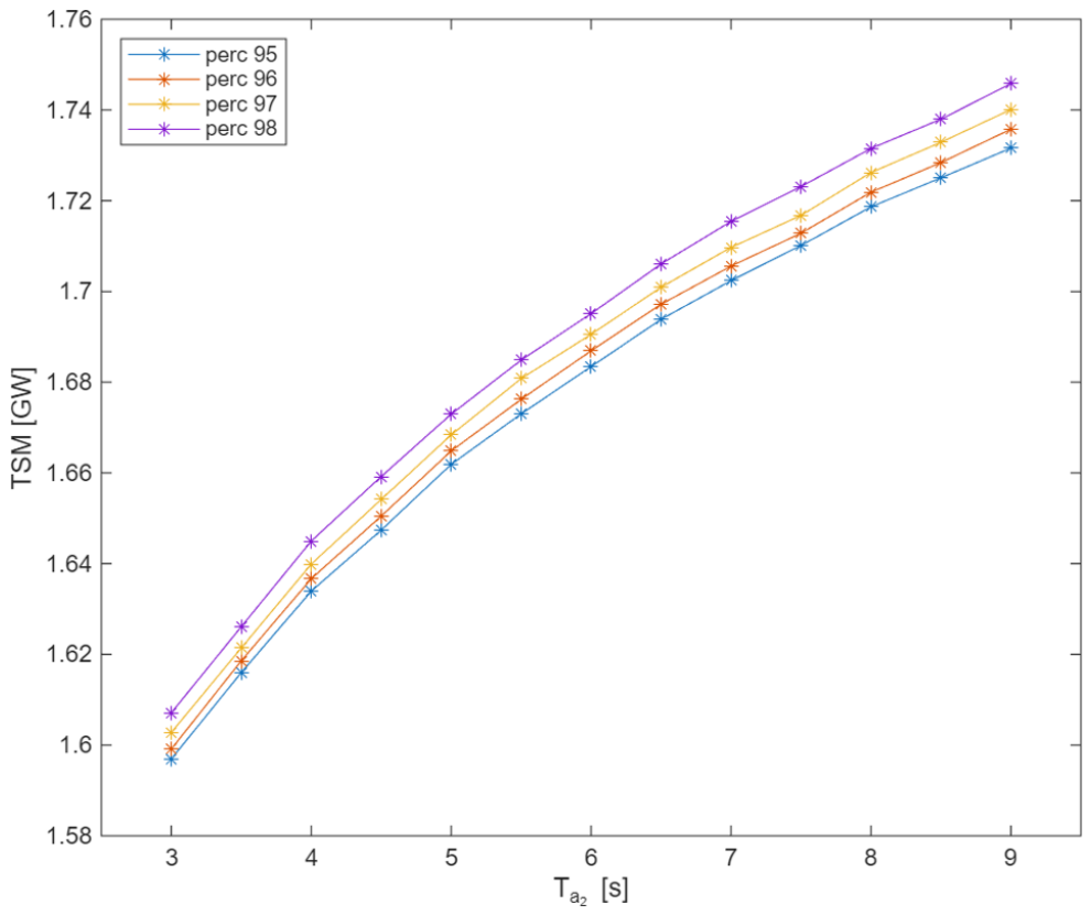
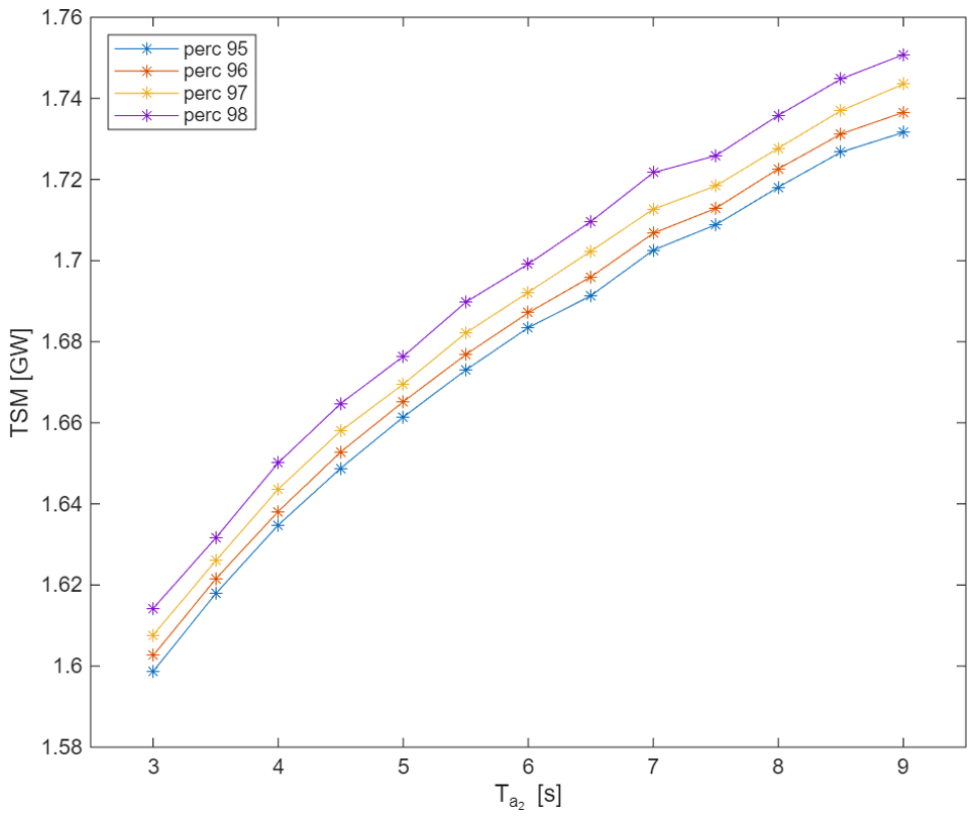
On the other hand, assuming a higher inertia PDF mean value for the second area as $\mathbb{E}\left[{T_a}_2\right]=9 \mathrm{s}$ (Figure 13), the mean value of TSM increases to 1.68 GW with a standard deviation of 29.1 MW. This is due to the total PDF inertia value, that, with the higher contribution of second area, reaches $\mathbb{E}\left[T_{a_{eq}}\right]=3.56 \mathrm{s}$ and ${\sigma }_{{T_a}_{eq}}\cong 0.43 \mathrm{s}$ with respect to that of the previous cases. The dependence of TSM with different values of PDF of inertia of the second area is considerable from Figure 14 in which the variation in different percentile values of TSM are shown as a function of mean values of inertia of the second area.

For the typical inertia range 3–9 s, the 95% percentile of TSM obtained ranges from 1.60 to 1.73 GW. The same consideration can be given in cases in which the inertia PDF variables are assumed as a gamma multivariate distribution. Figure 15 shows this result for case with $\mathbb{E}\left[{T_a}_1\right]=6 \mathrm{s}$ and $\mathbb{E}\left[{T_a}_2\right]=3 \mathrm{s}$, assuming a ${CV}_{{T_a}_2}\cong 0.167$.

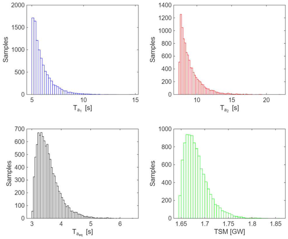
In this case a total inertia PDF variable with $\mathbb{E}\left[T_{a_{eq}}\right]= 1.98 \mathrm{s}$ and ${\sigma }_{{T_a}_{eq}}\cong 0.22 \mathrm{s}$ and a TSM PDF variable with $\mathbb{E}\left[TSM\right]= 1.56 \mathrm{G}\mathrm{W}$ and ${\sigma }_{TSM}\cong 20 \mathrm{M}\mathrm{W}$ are obtained. In the same condition with a $\mathbb{E}\left[{T_a}_2\right]=9 \mathrm{s}$ a total inertia PDF variable with $\mathbb{E}\left[T_{a_{eq}}\right]=3.56 \mathrm{s}$ and ${\sigma }_{{T_a}_{eq}}\cong 0.38 \mathrm{s}$ occurs and a TSM PDF variable with $\mathbb{E}\left[TSM\right]=1.68 \mathrm{G}\mathrm{W}$ and ${\sigma }_{TSM}\cong 25 \mathrm{M}\mathrm{W}$ is obtained (Figure 16).

In Figure 17 the variation in TSM percentiles as a function of inertia mean values of second areas is shown. The increase in inertia of second area leads to an increase in TSM that for a percentile of 95% ranges from the value of 1.60 GW to 1.73 GW.

5.3. Case C—Not Independent Inertias

Finally, case C is illustrated in this section, where for sake of brevity only the case of equal means will be considered.

It is recalled that the correlation coefficient (CC) may assume values from −1 to +1, and a negative CC for the two areas RESS’s could mean that while the RSS in one area tends to increase, the other tends to decrease, a situation which may occur depending on different adopted strategies or even weather conditions.

Assuming a lognormal PDF for the inertia variable of each on two areas of the power system with the same characteristics reported in case A, this investigation introduces a correlation between two inertia variables with a correlation coefficient ${\rho }_{1,2}$ variable in the range between $-0.9$ and $0.9$.

Figure 18 shows results for ${\rho }_{1,2}=-0.9$. In this case a total inertia PDF variable with $\mathbb{E}\left[T_{a_{eq}}\right]=2.93 \mathrm{s}$ and ${\sigma }_{{T_a}_{eq}}\cong 0.12 \mathrm{s}$ occurs and a TSM PDF variable with mean value of 1.638 GW and a standard deviation of 8.9 MW is obtained.

Instead, for a ${\rho }_{1,2}=0.9$ the mean value $\mathbb{E}\left[T_{a_{eq}}\right]=3.00 \mathrm{s}$ and the standard deviation ${\sigma }_{{T_a}_{eq}}\cong 0.49 \mathrm{s}$ occurs and a TSM PDF variable with mean value of about 1. 643 GW and a standard deviation of about 35.7 MW is obtained (Figure 19).

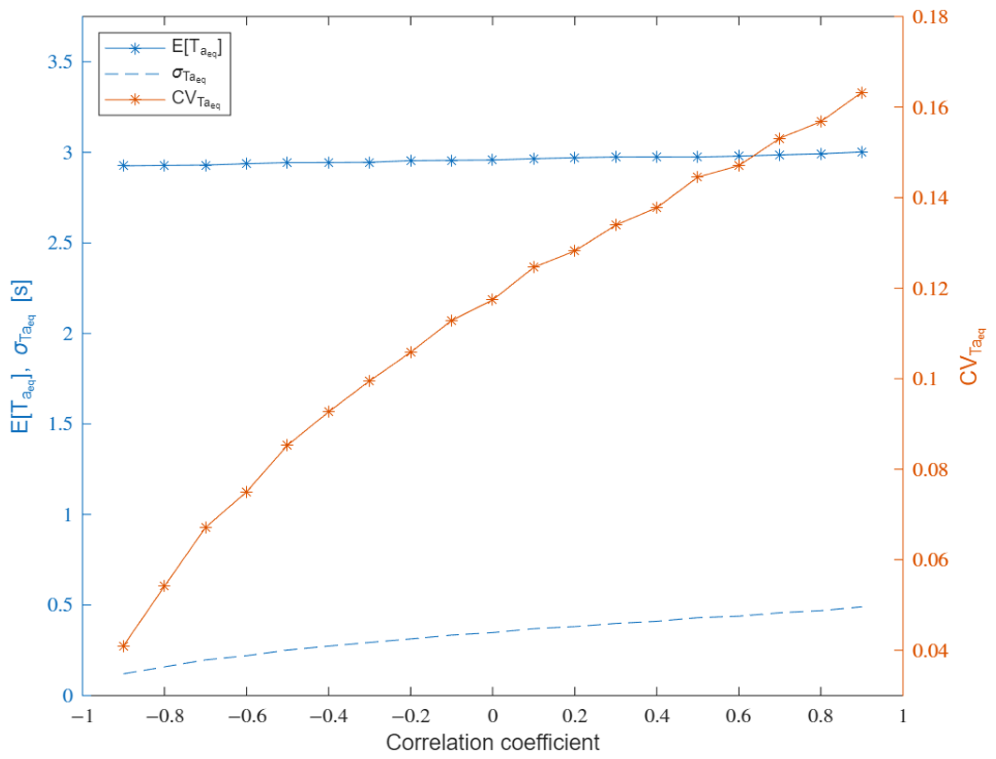
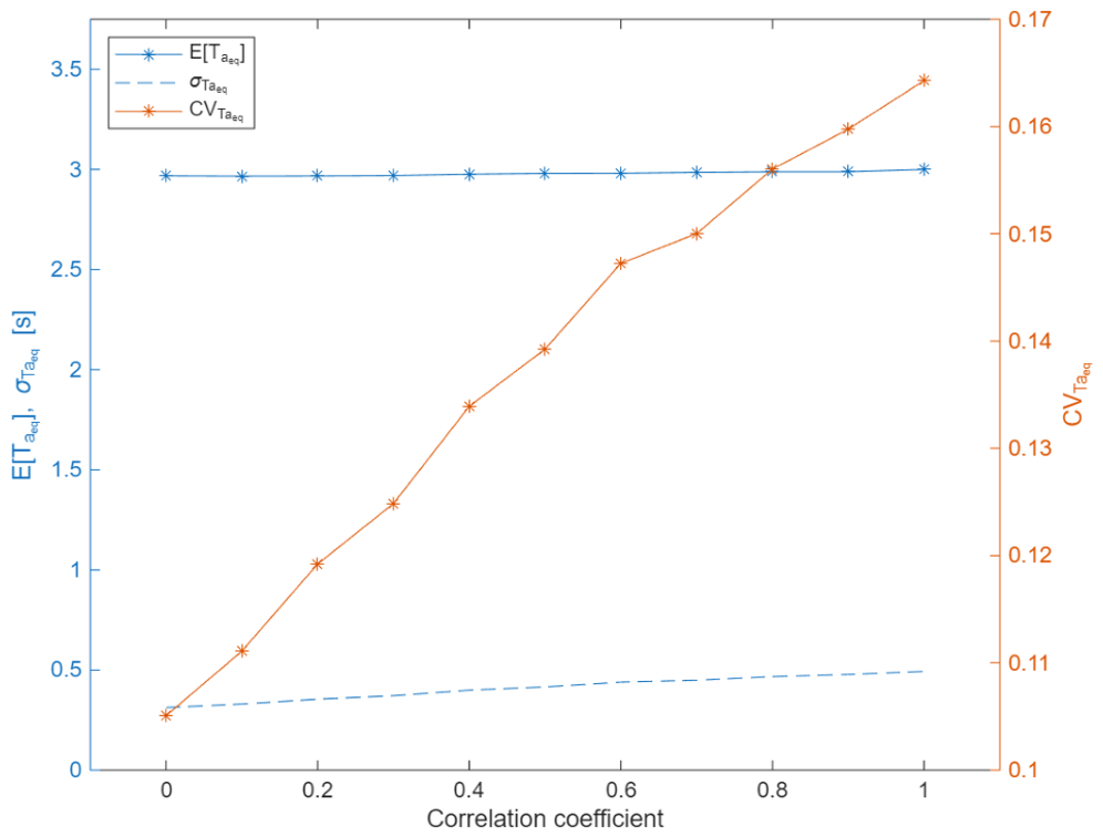
The impact of the correlation between random variables of inertia of the two areas ${T_a}_1$ and ${T_a}_2$ on the ${T_a}_{eq}$ is more important on random variable dispersion than on its mean value. In Figure 20, assuming a lognormal multivariate distribution for ${T_a}_1$ and ${T_a}_2$, the parameters $\mathbb{E}\left[T_{a_{eq}}\right]$, ${\sigma }_{{T_a}_{eq}}$ and ${CV}_{{T_a}_{eq}}$ that characterize the random variable $T_{a_{eq}}$ are shown.

The standard deviation ${\sigma }_{{T_a}_{eq}}$ changes from a value of 0.12 s to a value of 0.35 s as a function of correlation coefficient between the inertias of the two areas, ranging from −0.9 to 0, and from 0.35 s to a value of 0.49 s for correlation coefficient ranging from 0 to 0.9, with a monotone trend.

There is the same relationship between $\mathbb{E}\left[T_{a_{eq}}\right]$ and the correlation coefficient, but with a less steep slope (from 2.93 s to 2.96 s and to 3 s for −0.9–0 and 0–0.9 ranges of correlation coefficient, respectively). The parameter ${CV}_{{T_a}_{eq}}$ increases from 0.04 to 0.12 and to 0.16 with the rise in correlation coefficient from −0.9 to 0 and from 0 to 0.9, respectively. The same result is obtained for a gamma multivariate distribution of random variables of inertia of the two areas ${T_a}_1$ and ${T_a}_2$ as visible in Figure 21.

In this second case the standard deviation ${\sigma }_{{T_a}_{eq}}$ ranges from 0.31 s to 0.49 s in relation to coefficient correlation variation from 0 to 1, while $\mathbb{E}\left[T_{a_{eq}}\right]$ ranges from 2.97 s to 3 s. Also, in this case the ${\sigma }_{{T_a}_{eq}}$ is characterized by a steeper slope than $\mathbb{E}\left[T_{a_{eq}}\right]$ as verified from ${CV}_{{T_a}_{eq}}$ that increases from 0.11 to 0.16 for correlation coefficient variation from 0 to 1. Therefore, the correlation coefficient variation has a low effect on mean value, but a greater effect on standard deviation: the increase in correlation between two areas’ inertias leads to a greater increase the random variable dispersion than its mean value.

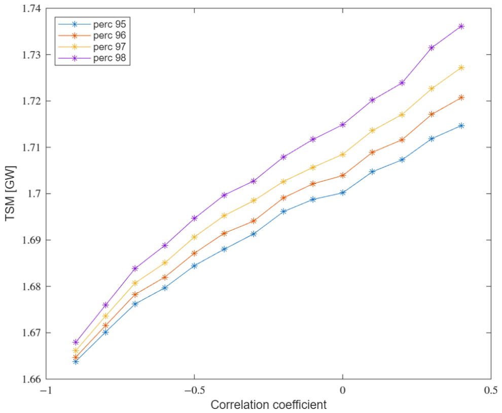
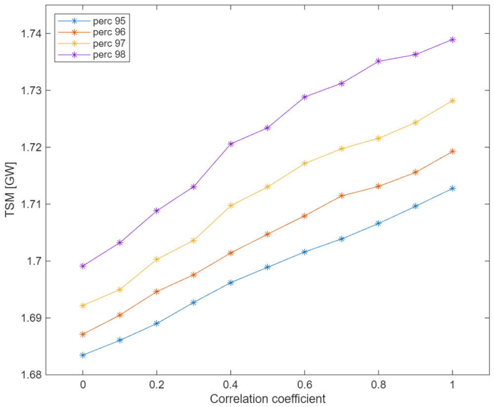
Figure 22 shows the variation in different percentile values of TSM probability densities obtained with ${\rho }_{1,2}$ variation: the negative correlation between inertia values of two areas is an index of opposite behaviors in transient phases leading to a reduction in TSM with respect to the positive correlation. The 95% percentile is characterized by a variation in its value for correlation coefficient range −0.9–0 of about 31 MW and in the range 0–0.9 of about 21 MW. Although the impact of the correlation coefficient on the TSM, as derived from the results shown in Figure 7, Figure 18, Figure 19 and Figure 20, is very low (all values reported are very close to 1.64 GW), it mainly affects the standard deviation of the TSM, which varies from 8.9 MW (correlation coefficient equal to −0.9) to 35.7 MW (correlation coefficient of 0.9). Assuming a gamma multivariate inertia variables distribution with a correlation coefficient of 0.5, $\mathbb{E}\left[T_{a_{eq}}\right]=2.98 \mathrm{s}$ and ${\sigma }_{{T_a}_{eq}}\cong 0.42 \mathrm{s}$ occur and a TSM PDF variable with mean value of 1.64 GW and a standard deviation of 29 MW is obtained (Figure 23).

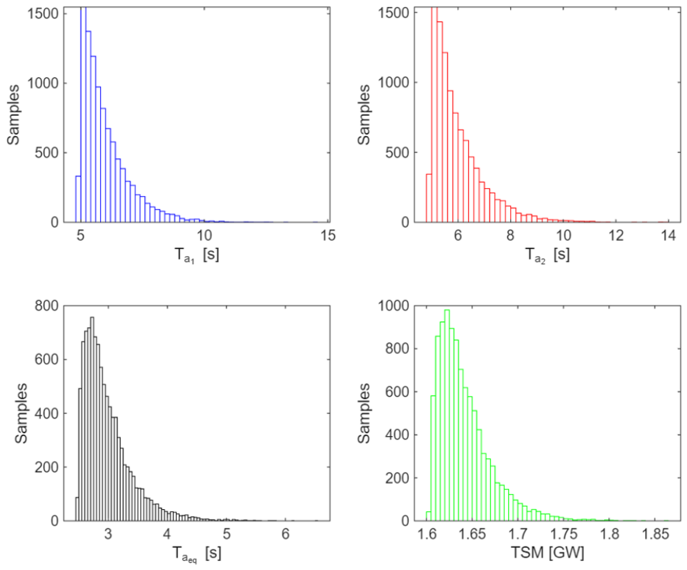
Figure 24 shows the results for the case in which the correlation coefficient between the PDFs of the inertia variables of the two areas is assumed to reach the maximum value of 1. In this condition, the two PDFs of the inertia variables for the two areas, at up in left and right sides of Figure 24, are almost identical; consequently, a PDF of the total inertia (at bottom in left side of Figure 24) is obtained that almost coincides with them. Its mean value $\mathbb{E}\left[T_{a_{eq}}\right]=3 \mathrm{s}$ and its standard deviation ${\sigma }_{{T_a}_{eq}}\cong 0.42 \mathrm{s}$. The TSM obtained has $\mathbb{E}\left[TSM\right]=1.64 \mathrm{G}\mathrm{W}$ and ${\sigma }_{TSM}\cong 34 \mathrm{M}\mathrm{W}$. Figure 25 shows the different percentile values of TSM probability densities obtained with ${\rho }_{1,2}$ variation in the range of 0–1.

Similarly with lognormal multivariate distribution, also in this case a greater correlation coefficient led to increase in TSM. The 95% percentile is characterized by a variation in its value for correlation coefficient range 0–1 is of about 29 MW according to results for lognormal multivariate distribution.

6. Conclusions

The paper provides a rigorous probabilistic framework for assessing transient stability in low-inertia and renewable-rich grids. Indeed, the variability of rotational inertia in interconnected power systems affects their transient stability margins. As modern grids increasingly integrate converter-based renewable generation, system inertia becomes both lower and more uncertain, introducing faster electromechanical dynamics and raising concerns for operational security. In this paper the transient stability is modeled as a boundary value problem, applying the equal area criterion to determine the maximum transferable power that preserves synchronism after a disturbance. The paper derives the TSM as a nonlinear function of system reactances and inertia and shows how the entire post-fault trajectory can be expressed through explicit Euler integration. The probabilistic characterization of TSM is used when inertia is treated as a random variable. Monte Carlo simulations demonstrate that, for realistic parameter ranges, TSM depends almost linearly on inertia, a result supported by analytical approximations of the swing equation. The methodology is applied to a two-area system, where each area has its own stochastic inertia. The equivalent system inertia is computed through a harmonic-mean relationship, and its distribution is analyzed under both correlated lognormal and gamma models. Results show that inertia correlation has limited influence on the expected value of the TSM but significantly affects its dispersion: higher correlation increases the variance of both equivalent inertia and TSM. Numerical case studies confirm that the randomness of inertia can alter stability margins.

The paper offers insights relevant to planning, risk assessment, and future multiarea extensions.

References

1. ENTSO-E. The Inertia Challenge in Europe—Present and Long-Term Perspective Insight Report. Ten-Year Network Development Plan (TYNDP 2020), August, 2021. Available online: https://eepublicdownloads.blob.core.windows.net/public-cdn-container/tyndp-documents/TYNDP2020/FINAL/entso-e_TYNDP2020_Insight_Report_Inertia_2108.pdf (accessed on 1 February 2026).
2. ENTSO-E. Project Inertia-Phase II: Updated Frequency Stability Analysis in Long Term Scenarios, Relevant Solutions and Mitigation Measures from: ENTSO-E Updated Frequency Stability Analysis in Long Term Scenarios, Relevant Solutions and Mitigation Measures. November 2023, pp. 1–33. Available online: www.entsoe.eu (accessed on 1 February 2026).
3. Ratnam, K.S.; Palanisamy, K.; Yang, G. Future low-inertia power systems: Requirements, issues, and solutions—A review. Renew. Sustain. Energy Rev. 2020, 124, 109773. [Google Scholar] [CrossRef] [Scilit]
4. Zhang, W.; Wen, Y.; Chung, C.Y. Inertia Security Evaluation and Application in Low-Inertia Power Systems. IEEE Trans. Power Syst. 2024, 40, 1725–1737. [Google Scholar] [CrossRef] [Scilit]
5. Zhang, G.; Ren, J.; Zeng, Y.; Liu, F.; Wang, S.; Jia, H. Security assessment method for inertia and frequency stability of high proportional renewable energy system. Int. J. Electr. Power Energy Syst. 2023, 153, 109309. [Google Scholar] [CrossRef] [Scilit]
6. Milano, F.; Dorfler, F.; Hug, G.; Hill, D.J.; Verbič, G. Foundations and challenges of low-inertia systems (Invited Paper). In Proceedings of the 20th Power Systems Computation Conference, PSCC 2018, Dublin, Ireland, 11–15 June 2018; pp. 1–25. [Google Scholar] [CrossRef] [Scilit]
7. Tielens, P.; Van Hertem, D. The relevance of inertia in power systems. Renew. Sustain. Energy Rev. 2016, 55, 999–1009. [Google Scholar] [CrossRef] [Scilit]
8. Song, J.; Zhou, X.; Zhou, Z.; Wang, Y.; Wang, Y.; Wang, X. Review of Low Inertia in Power Systems Caused by High Proportion of Renewable Energy Grid Integration. Energies 2023, 16, 6042. [Google Scholar] [CrossRef] [Scilit]
9. Bruno, S.; Giannoccaro, G.; Iurlaro, C.; La Scala, M.; Rodio, C. A Low-cost Controller to Enable Synthetic Inertia Response of Distributed Energy Resources. In Proceedings of the 2020 IEEE International Conference on Environment and Electrical Engineering and 2020 IEEE Industrial and Commercial Power Systems Europe (EEEIC/I&CPS Europe), Madrid, Spain, 9–12 June 2020. [Google Scholar] [CrossRef] [Scilit]
10. Istrate, R.A.; Toma, L.; Dobrin, B.P. Impact of Mechanical Inertia on the Power System Stability. In Proceedings of the 2022 12th International Conference and Exposition on Electrical and Power Engineering (EPE 2022), Iasi, Romania, 20–22 October 2022; pp. 639–643. [Google Scholar] [CrossRef] [Scilit]
11. Chiodo, E.; Lauria, D.; Mottola, F. On-Line Bayes Estimation of Rotational Inertia for Power Systems with High Penetration of Renewables. Part I: Theoretical Methodology. In Proceedings of the 2018 International Symposium on Power Electronics, Electrical Drives, Automation and Motion (SPEEDAM 2018), Amalfi, Italy, 20–22 June 2018; pp. 835–840. [Google Scholar] [CrossRef] [Scilit]
12. Wu, Q.H.; Lin, Y.; Hong, C.; Su, Y.; Wen, T.; Liu, Y. Transient Stability Analysis of Large-scale Power Systems: A Survey. CSEE J. Power Energy Syst. 2023, 9, 1284–1300. [Google Scholar] [CrossRef] [Scilit]
13. Tian, M.; Ren, Z.; Xing, D.; Jiang, Y. Influence of system inertia time constant on transient stability level of AC power grid. Electron. Lett. 2023, 59, e12978. [Google Scholar] [CrossRef] [Scilit]
14. Mishan, R.; Fu, X.; Hingu, C.; Ben-Idris, M. Impacts of Inertia and Photovoltaic Integration on Existing and Proposed Power System Transient Stability Parameters. Energies 2025, 18, 2915. [Google Scholar] [CrossRef] [Scilit]
15. Chiodo, E.; Lauria, D.; Pisani, C.; Villacci, D. Transient stability margins evaluation based upon probabilistic approach. Int. Rev. Electr. Eng. 2013, 8, 752–761. Available online: https://www.praiseworthyprize.org/jsm/index.php?journal=iree&page=article&op=view&path%5B%5D=10310 (accessed on 1 February 2026).
16. Fang, L.; Ji-lai, Y. Transient stability analysis with equal area criterion directly used to a non-equivalent generator pair. In Proceedings of the 2009 2nd International Conference on Power Engineering, Energy and Electrical Drives (POWERENG 2009), Lisbon, Portugal, 18–20 March 2009; pp. 386–389. [Google Scholar] [CrossRef] [Scilit]
17. Shi, Q.; Xu, Y.; Sun, Y.; Feng, W.; Li, F.; Sun, K. Analytical Approach to Estimating the Probability of Transient Stability under Stochastic Disturbances. In Proceedings of the 2018 IEEE Power & Energy Society General Meeting (PESGM 2018), Portland, OR, USA, 5–10 August 2018; pp. 1–5. [Google Scholar] [CrossRef] [Scilit]
18. Chiodo, E.; Lauria, D. Transient stability evaluation of multimachine power systems: A probabilistic approach based upon the extended equal area criterion. IEE Proc. Gener. Transm. Distrib. 1994, 141, 545–553. [Google Scholar] [CrossRef] [Scilit]
19. Hua, K.; Mishra, Y.; Ledwich, G. Fast Unscented Transformation-Based Transient Stability Margin Estimation Incorporating Uncertainty of Wind Generation. IEEE Trans. Sustain. Energy 2015, 6, 1254–1262. [Google Scholar] [CrossRef] [Scilit]
20. Mathai, A.M.; Moschopoulos, P.G. On a Multivariate Gamma. J. Multivar. Anal. 1991, 39, 135–153. [Google Scholar] [CrossRef] [Scilit]
21. Nocedal, J.; Wright, S.J. Numerical Optimization, 2nd ed.; Springer Series in Operations Research and Financial Engineering; Springer: New York, NY, USA, 2006. [Google Scholar]
Figure 1. Electrical system connected via passive double three-phase line to a node assumed to have infinite short-circuit power (infinite power bus).
Energies 19 02737 g001
Figure 2. Equal area criterion for a synchronous generator connected to an infinite bus; in the figure δ f = δ ( Δ t c l ) and δ r = δ Δ t c l +   Δ t r .
Energies 19 02737 g002
Figure 3. Two electrical system areas connected via passive double three-phase line.
Energies 19 02737 g003
Figure 4. Stability margin curves as a function of fault location.
Energies 19 02737 g004
Figure 5. Stability margin curves for the four types of faults considered: single-phase line-to-ground fault (at the top on the left), two-phase fault (at the top on the right), line-to-ground double-phase fault (at the bottom on the left) and three-phase fault (at the bottom on the right) for the two-area system.
Energies 19 02737 g005
Figure 6. Equivalent inertia mean value μ T a e q curve as a function of correlation coefficient between multivariate lognormal random inertias of two power system areas.
Energies 19 02737 g006
Figure 7. Distributions of the random variables of power system inertia (at the top left) and of the phase angles ( δ 0 , δ f , δ r ) of the equivalent synchronous machine (at the top right and at the bottom left and right, respectively) for three-phase faults.
Energies 19 02737 g007
Figure 8. Distributions of the random area variables ( A f , A r and A m ) evaluated for equal area criterion for the equivalent synchronous machine (at the top left and right and at the bottom left, respectively) and the TSM related to this case at the right bottom for three-phase faults.
Energies 19 02737 g008
Figure 9. Distributions of the random area variables ( A f , A r and A m ) evaluated for equal area criterion for the equivalent synchronous machine (at the top left and right and at the bottom left, respectively) and the TSM related to this case at the right bottom for single-phase faults.
Energies 19 02737 g009
Figure 10. Distributions of the lognormal random inertia variables with the same means of the two areas and total power system (at the top left and right and at the bottom left, respectively) and of the TSM related to this case at the bottom right.
Energies 19 02737 g010
Figure 11. Distributions of the gamma random inertia variables with the same means of the two areas and total power system (at the top left and right and at the bottom left, respectively) and of the TSM related to this case at the bottom right.
Energies 19 02737 g011
Figure 12. Distributions of the lognormal random inertia variables with different means ( E T a 2 = 3   s ) of the two areas and total power system (at the top left and right and at the bottom left, respectively) and of the TSM related to this case at the right bottom.
Energies 19 02737 g012
Figure 13. Distributions of the lognormal random inertia variables with E T a 1 = 6   s and ( E T a 2 = 9   s ) and total power system (at the top left and right and at the bottom left, respectively). The TSM related to this case is shown at the right bottom.
Energies 19 02737 g013
Figure 14. The 95%, 96%, 97% and 98% percentile values of TSM Distributions as a function of the lognormal random inertia variable values of the second area.
Energies 19 02737 g014
Figure 15. Distributions of multivariate gamma random inertia variables with E T a 1 = 6   s and E T a 2 = 3   s and of total power system (at the top left and right and at the bottom left, respectively); the TSM related to this case is shown at the right bottom.
Energies 19 02737 g015
Figure 16. Distributions of the gamma random inertia variables of two areas ( E T a 1 = 6   s and E T a 2 = 9   s ) and of the total power system (at the top left and right and at the bottom left, respectively) and of the TSM related to this case at the right bottom.
Energies 19 02737 g016
Figure 17. The 95%, 96%, 97% and 98% percentile values of TSM Distributions as a function of the gamma random inertia variable values of the second area.
Energies 19 02737 g017
Figure 18. Distributions of the lognormal multivariate random inertia variables of the two areas and of total power system (at the top left and right and at the bottom left, respectively) assuming ρ 1 , 2 = 0.9 between inertia of the two areas; the related TSM is visible at the right bottom.
Energies 19 02737 g018
Figure 19. Distributions of the lognormal random inertia variables of the two areas and total power system (at the top left and right and at the bottom left, respectively) assuming a correlation coefficient ρ 1 , 2 = 0.9 between inertia of the two areas, and of the TSM related to this case at the right bottom.
Energies 19 02737 g019
Figure 20. Probability parameters of the equivalent inertia random variable ( T a e q ) as a function of correlation coefficient between the multivariate inertia random variables of two areas of investigated power system with a lognormal distribution.
Energies 19 02737 g020
Figure 21. Probability parameters of the equivalent inertia random variable ( T a e q ) as a function of correlation coefficient between the multivariate inertia random variables of two areas of investigated power system with a gamma distribution.
Energies 19 02737 g021
Figure 22. The 95%, 96%, 97% and 98% percentile values of TSM Distributions as a function of the correlation coefficient between the lognormal random inertia variables of the two areas.
Energies 19 02737 g022
Figure 23. Distributions of the gamma random inertia variables of the two areas and total power system (at the top left and right and at the bottom left, respectively) assuming a correlation coefficient ρ 1 , 2 = 0.5 between inertia of the two areas, and of the TSM related at the right bottom.
Energies 19 02737 g023
Figure 24. Distributions of the multivariate gamma random inertia variables of the two areas and of the total power system (at the top left and right and at the bottom left, respectively) assuming ρ 1 , 2 = 1 , and the related distribution of the TSM at the right bottom.
Energies 19 02737 g024
Figure 25. The 95%, 96%, 97% and 98% percentile values of TSM Distributions as a function of the correlation coefficient between the gamma random inertia variable values of the two areas.
Energies 19 02737 g025