Article

PINN-Inspired Topology-Aware Learning for Harmonic State Recognition in Multi-Node Coupled Systems

1
Electric Power Institute, Yunnan Power Grid Company Ltd., Kunming 650217, China
2
State Key Laboratory of Power Transmission Equipment Technology, Chongqing University, Chongqing 400044, China
*
Author to whom correspondence should be addressed.
Energies 2026, 19(11), 2564; https://doi.org/10.3390/en19112564 (registering DOI)
Submission received: 11 April 2026 / Revised: 6 May 2026 / Accepted: 15 May 2026 / Published: 26 May 2026
(This article belongs to the Special Issue Technology for Analysis and Control of Power Quality)

Abstract

Accurate dynamic state reconstruction in complex multi-node coupled systems is critical for ensuring operational stability and reliability. However, this task is highly challenging due to spatially sparse measurement sensors, strong dynamic coupling among nodes, and the intractability of explicitly modeling the underlying physical mechanisms. Conventional data-driven methods exhibit limited generalization under sparse labels or out-of-distribution conditions, whereas strict physics-driven solvers often fail to converge in complex environments with unmodeled dynamics. To address these limitations, this paper proposes a physics-informed neural network (PINN)-inspired topology-aware learning framework for multi-node state reconstruction. Rather than acting as a strict physical equation solver, the proposed method innovatively injects physical priors into data-driven temporal modeling. By incorporating physical consistency constraints, latent dynamic regularization, topology-aware priors, and an observer-style multi-branch hybrid fusion strategy, the framework effectively overcomes the drawbacks of single-paradigm models to enhance estimation accuracy and robustness. Extensive experiments on real-world coupled system data demonstrate that the proposed framework outperforms state-of-the-art linear, tree-based, and pure sequential models. Specifically, the proposed topology-aware hybrid observer achieves a Root Mean Square Error (RMSE) ≈ 0.02604 and an R 2 0.79060 on the multi-node harmonic reconstruction task, demonstrating superior accuracy and dynamic tracking capability compared to the other baselines. Furthermore, cross-node virtual sensing and ablation experiments verify that the constructed physics-guided observer achieves stable cross-node reconstruction under limited physical observations. The results indicate that integrating PINN-inspired learning with topology-aware modeling provides a highly robust and feasible paradigm for ubiquitous sensing and state estimation in complex networks under restricted measurement conditions.

1. Introduction

The paradigm shift towards sustainable energy has fundamentally redefined the architectural and dynamic characteristics of modern electrical grids, driving a rapid proliferation of inverter-based resources (IBRs) [1]. In this evolving landscape, large-scale offshore wind farms (OWFs) stand out as quintessential examples of complex multi-node coupled networks. While these marine installations are crucial for harnessing massive and consistent wind energy, their integration presents profound stability and power quality challenges. Replacing conventional synchronous machines with power-electronic interfaces intrinsically reduces system inertia and transitions the primary stability concerns from low-frequency electromechanical oscillations to intricate, broadband electromagnetic dynamics [2,3].
A critical bottleneck in operating such sprawling coupled systems lies in the pervasive harmonic resonance induced by complex spatial topologies and active control components. The dense deployment of converter-interfaced generators injects highly dynamic, non-sinusoidal currents into the grid. When these emissions interact with the frequency-dependent impedances of the network, specifically, the distributed capacitance of extensive submarine transmission cables and the inductance of grid transformers, they form severe multi-node resonance loops [4,5]. The recent literature highlights that these harmonic behaviors are highly non-stationary, heavily modulated by time-varying meteorological conditions and the continuous adjustment of aerodynamic operating points [6]. Consequently, minor perturbations can rapidly amplify into severe voltage and current distortions that propagate across the entire network topology.
Prolonged exposure to such high-frequency distortions accelerates insulation degradation and triggers severe localized thermal stress, ultimately jeopardizing grid reliability [7]. To proactively mitigate these risks, continuous and accurate harmonic state reconstruction across all system nodes is imperative. However, achieving full observability is highly constrained by the spatial sparsity of expensive physical sensors in remote marine environments. Current monitoring mechanisms remain predominantly reactive, relying on rigid threshold alarms that fail to capture the subtle dynamic evolutions characterizing the sub-health states of system [8]. While pure data-driven state estimation models have been extensively explored, they exhibit significant vulnerabilities, notably poor generalization under sparse labels and out-of-distribution shifts [9]. Conversely, strict physics-based analytical solvers often fail to converge in complex environments due to the intractability of explicitly formulating high-dimensional, unmodeled dynamics [10].
Recently, physics-informed neural networks (PINNs) have emerged as a transformative approach in dynamic system modeling, demonstrating remarkable success in embedding physical laws directly into neural network training to enhance state estimation under noisy or partial observations [11]. Inspired by these advancements, but recognizing the limitations of standard continuous PINNs in handling large-scale discrete network topologies, this paper introduces a novel PINN-inspired topology-aware learning framework. By innovatively injecting physical consistency constraints and topological priors into a data-driven observer architecture, the proposed method overcomes the limitations of single-paradigm models, enabling highly robust multi-node harmonic state reconstruction under severely limited measurement conditions.

1.1. Prior Works and Motivations

Accurate harmonic state estimation has become a fundamental requirement for the stable operation of inverter-based grids [12,13], largely driven by the global integration of renewable energy and power-electronic interfaces [14,15,16]. Early works extended multi-frequency state estimation to network-level harmonic analysis [17], demonstrating that observability and measurement quality critically dictate estimation accuracy [18]. Meanwhile, strict international grid codes continue to enforce rigorous harmonic compliance [19,20]. Concurrently, model-driven approaches have extensively investigated harmonic resonance utilizing modal and impedance analysis [4,21]. These studies reveal that resonance risks in OWFs are highly sensitive to submarine cable capacitance [22,23], converter control behaviors [24], and frequency-coupled impedance [25]. While these classical methods provide crucial theoretical foundations for recovering unmeasured harmonics, these predominantly rely on explicit system models and ideal measurement conditions. Such prerequisites are rarely satisfied in OWFs, which are characterized by partial observability and incomplete physical records.
To address these modeling complexities, deep learning (DL) sequence architectures have been increasingly adopted [26]. For instance, long short-term memory (LSTM) networks are widely applied to capture short-term temporal harmonic variations [27,28,29], while advanced Transformers excel at modeling long-range, non-stationary dynamic states [30,31,32]. Furthermore, recent advances in topology-aware learning have shown that explicitly incorporating network structures improves state estimation in partially observable grids [33,34], especially when integrated with domain knowledge [35]. This is vital for OWFs, as harmonic behaviors are not strictly local phenomena and cross-node coupling and propagation along the collection grid significantly affect harmonic levels. However, existing topology-aware research predominantly focuses on fundamental-frequency power flow or voltage estimation, leaving multi-node harmonic state reconstruction largely unexplored.
Additionally, PINNs and related physics-guided methods have gained traction for integrating data fitting with physical priors [36]. Their core advantage lies in enhancing model robustness under sparse or noisy observations. However, applying strict PINNs to real-world OWF harmonic reconstruction presents severe practical bottlenecks. In actual operational data, effective harmonic processes are simultaneously influenced by hidden converter dynamics, aggregated impedance behaviors, and measurement abstractions. Consequently, it is intractable to formulate explicit, closed-form governing equation residuals suitable for standard collocation training. Meanwhile, purely data-driven sequence models struggle with the extreme data imbalance of supervisory control and data acquisition (SCADA) systems, often overfitting to steady-state operations. To mitigate this, ensemble tabular learners, such as Random Forests [37,38] and gradient boosting variants [39,40], have been benchmarked for power system tasks due to their statistical robustness, though they inherently lack sequence memory. Although generative models can synthesize data to mitigate sparsity [41,42], they risk introducing unphysical artifacts [43]. Moreover, these conventional frameworks generally lack the capability of “virtual sensing”, estimating the dynamic states of unmonitored nodes based on sparse adjacent observations.
To systematically bridge these gaps, this paper proposes a PINN-inspired topology-aware learning framework for multi-node harmonic state reconstruction. Rather than claiming to construct a strictly parameterized partial differential equation (PDE)-solving PINN, we adopt the pragmatic philosophy of injecting physical knowledge into the learning process. By embedding physical consistency constraints and topological priors into a data-driven temporal observer, the proposed hybrid fusion architecture effectively captures the multi-node coupling characteristics. This framework uniquely unifies harmonic physical consistency, offshore node coupling structures, and observer-oriented virtual sensing, enabling stable multidimensional state reconstruction even under conditions of measurement sparsity and limited label diversity.

1.2. Contributions

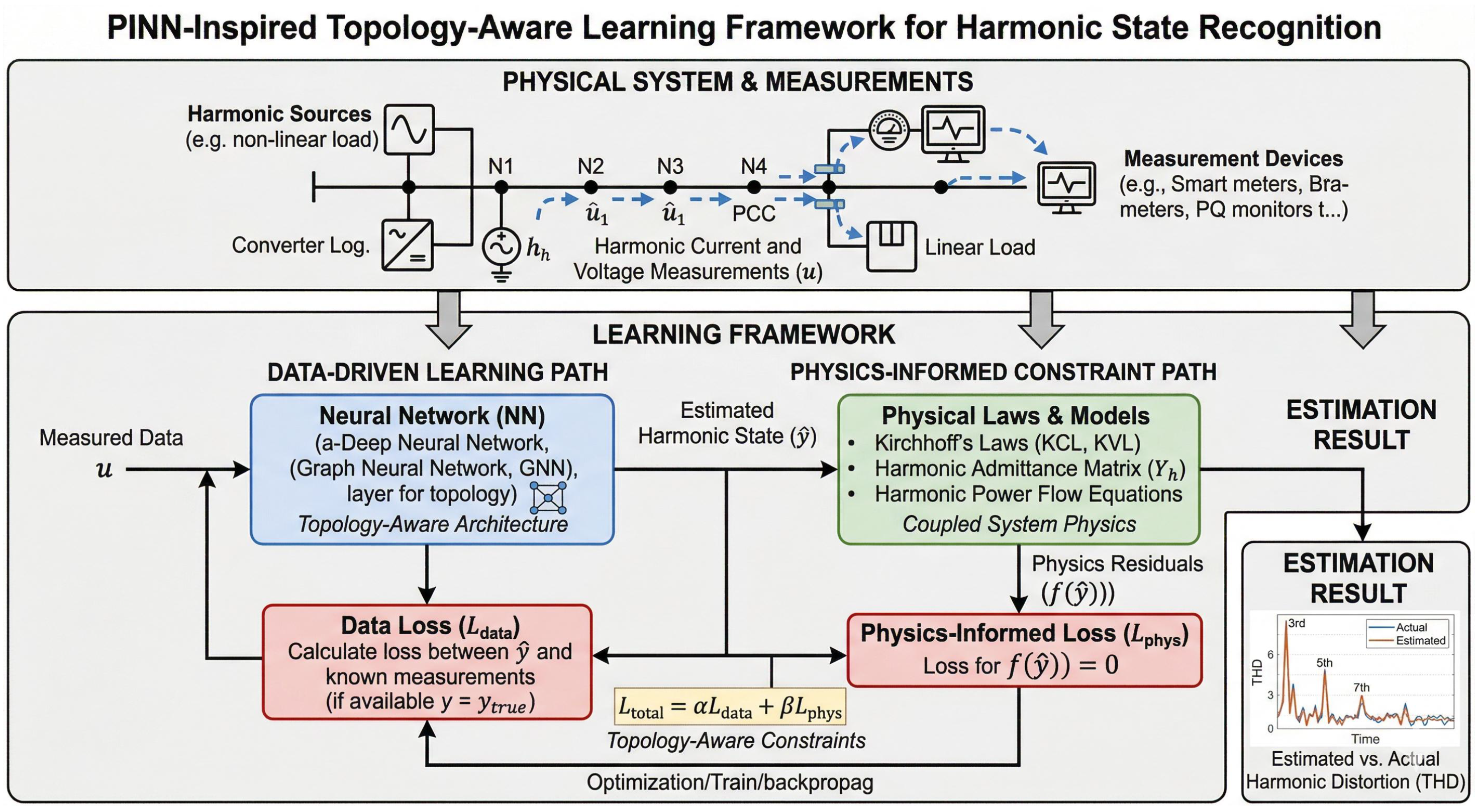
As analyzed above, harmonic state reconstruction in complex coupled networks is not a standard time-series forecasting problem, primarily due to inherent multi-node couplings and partial observability. While existing datasets may be insufficient to support strict physical equation solvers, they are adequate for training data-driven frameworks regularized by physical principles and statistical priors. Therefore, rather than claiming a strictly parameterized physical solver, this paper proposes a pragmatic PINN-inspired topology-aware learning framework. This approach systematically integrates data-driven temporal reconstruction, physics-guided objectives, and topology-aware priors to improve both estimation accuracy and system observability. The overall architecture and information flow of the proposed framework are illustrated in Figure 1.
The main contributions are summarized as follows:
  • PINN-Inspired Framework for Intractable Physical Systems: Unlike standard continuous PINNs that rely on explicitly formulated partial differential equations, which are generally intractable for complex, highly coupled offshore wind farm dynamics, we propose a novel, pragmatic learning paradigm. By embedding harmonic consistency constraints and latent dynamic regularization into the loss function, the framework successfully regularizes data-driven networks using underlying physical laws, circumventing the convergence failures of strict equation solvers in noisy environments.
  • Topology-Aware Hybrid Observer Design: Rather than merely concatenating existing algorithms, we design a topology-aware hybrid fusion architecture to bridge the gap between physical propagation and statistical learning. This observer-style structure organically integrates the non-stationary temporal memory of deep sequence models with the statistical robustness of tree-based tabular learners. Guided by spatial asymmetric priors, this fusion mechanism mathematically resolves the severe node-to-node coupling effects that single-paradigm models fail to capture.
  • Cross-Node Virtual Sensing Capability: The fundamental engineering novelty of the proposed framework lies in addressing the pervasive spatial sparsity of physical sensors in marine environments. Moving beyond conventional single-node regression, we demonstrate that the constructed physics-guided observer achieves reliable cross-node virtual sensing. It stably infers and reconstructs the dynamic harmonic states of physically unmonitored turbines by exploiting the topological dependencies of adjacent coupled measurements.
  • Transparent Benchmarking on Meteorological-Driven Simulations: To ensure rigorous validation and reproducibility, the framework is comprehensively evaluated using high-fidelity multi-node electrical simulations driven by real-world Turkish meteorological datasets. Experimental results confirm that the hybrid observer achieves superior multidimensional reconstruction accuracy compared to state-of-the-art baselines. Furthermore, the implementation source code and an executable sample dataset are open-sourced to guarantee transparency and facilitate independent verification.
The remainder of this paper is organized as follows. Section 2 formulates the multi-node harmonic state reconstruction problem and introduces the system topology. Section 3 details the proposed PINN-inspired topology-aware learning framework, including the physics-guided objectives and the hybrid observer-style fusion strategy. Section 4 presents a comprehensive experimental analysis, evaluating the main reconstruction performance, ablation studies, cross-node virtual sensing, and robustness under sparse labels. Finally, Section 5 concludes the paper. The main abbreviations and mathematical symbols adopted in this study are summarized in Table 1 for ease of reference.

2. System Modeling and Problem Formulation

In this section, we establish the physical foundation for harmonic resonance in multi-node OWFs, abstract the electrical network into a mathematical graph, and formally define the state reconstruction task under partial observability.

2.1. Harmonic Resonance in Coupled Offshore Networks

Modern OWFs integrate a large number of converter-interfaced wind turbine generators (WTGs) connected through extensive submarine cable networks. The power-electronic converters inherent to doubly fed induction generators (DFIGs) act as active harmonic sources, injecting broad-spectrum, non-sinusoidal currents into the collection grid.
To describe the network-level harmonic interactions, the electrical collection system is formulated within the framework of established harmonic load flow methodologies [44,45]. In these rigorous treatments of harmonic analysis, the grid is typically represented by a decoupled nodal admittance matrix at each specific harmonic order h. Let I h C N denote the vector of harmonic current injections from the N nodes, and  V h C N denote the corresponding nodal harmonic voltages. Based on Kirchhoff’s circuit laws and multi-frequency load flow principles, the network is governed by the following linear algebraic relation:
I h = Y h V h
where Y h C N × N is the network admittance matrix at the h-th harmonic order. The elements of Y h are determined by the distributed capacitance C i j , series inductance L i j , and resistance R i j of the submarine cables, as well as the leakage inductance of grid transformers.
Specifically, Equation (1) explicitly demonstrates that the harmonic voltage at any node is heavily influenced by the off-diagonal coupling terms Y i j , h . To ensure the representativeness and general applicability of the presented setup, the network parameters and specific voltage levels are strictly adopted from established benchmark test systems for DFIG-based offshore wind farms [41]. A harmonic disturbance originating at the wind turbine generator (WTG) terminal (e.g., the 575 V node, which corresponds to the standard nominal stator voltage of commercial 1.5 MW Type-3 DFIGs) propagates through the radial collection topology and can be significantly amplified at the point of common coupling (PCC, e.g., the 60 kV node, representing a widely utilized medium-voltage standard for offshore collection grids). Furthermore, Y h is non-stationary in practice due to the continuous integration of dynamic converter control loops, making exact analytical solutions intractable and necessitating a data-driven formulation.

2.2. Graph-Theoretic Topology Modeling

To mathematically capture this spatial coupling for the downstream data-driven observer, the complex electrical topology of the OWF is abstracted into an undirected, weighted graph G = ( V , E , A ) . The components of the graph are formally defined as:
  • V = { v 1 , v 2 , , v N } denotes the set of N physical nodes, encompassing all WTG terminals and the PCC.
  • E V × V represents the set of submarine cable connections linking the nodes.
  • A R N × N is the weighted adjacency matrix. To reflect the actual electrical proximity, the edge weight A i , j is defined based on the fundamental-frequency branch admittance magnitude, where A i , j = | Y i j , 1 | if ( v i , v j ) E , and 0 otherwise.
Based on the adjacency matrix, the diagonal degree matrix D R N × N is defined as D i i = j = 1 N A i j . Consequently, the graph Laplacian matrix L , which encapsulates the structural properties of the spatial manifold, is given by:
L = D A
The Laplacian L provides a critical mathematical foundation for enforcing topology-aware physical consistency across interconnected nodes in the subsequent framework.

2.3. Problem Formulation and Feature Construction

In practical OWF SCADA systems, the node-level sensor measurements are often partially observable. To align with the physical topology of the benchmark system described in Section 2.1, we define specific indices for our measured variables based on the standard 60 kV and 575 V transformer configuration of the Bozcaada offshore wind farm model [41]. Specifically, the subscript 60 explicitly denotes the electrical parameters at the 60 kV PCC, and the subscript 575 denotes the parameters at the 575 V WTG terminal. Let the raw sensory vector at a discrete time step t be defined as:
s t = [ W S t , sin ( W D t ) , cos ( W D t ) , V 60 , t , I 60 , t , V 575 , t , I 575 , t ]
which encapsulates meteorological features (wind speed W S , wind direction W D ) and the fundamental-frequency electrical states (voltage V and current I) at both the aforementioned 60 kV PCC and the 575 V WTG terminal. To clarify the non-stationary periodic operating patterns driven by meteorological shifts, we explicitly encode calendar and diurnal cycles into a temporal positional vector γ t :
γ t = sin 2 π h t 24 , cos 2 π h t 24 , , sin 2 π d t 366 , cos 2 π d t 366
where h t , m t , and  d t denote the hour-of-day, month, and day-of-year, respectively. Accompanied by a binary observation indicator o t { 0 , 1 } representing data availability before interpolation, the final integrated feature vector is x t = s t , γ t , o t .
For each timestamp, we construct a sliding temporal observation window of length L { 24 , 72 } :
X t ( L ) = x t L + 1 , x t L + 2 , , x t
The target dynamic harmonic state to be reconstructed is the total harmonic distortion (THD) across multiple spatial nodes and electrical attributes, defined as a strictly non-negative vector:
y t = THDV 60 t , THDI 60 t , THDV 575 t , THDI 575 t R + 4
The objective of the multi-node harmonic state reconstruction is to learn a robust mapping function F Θ parameterized by Θ to estimate the global harmonic states y ^ t = F Θ X t ( L ) under the topological guidance of G . It is important to note that the investigated THD indices encompass broadband harmonic distortions up to the 50th harmonic order (i.e., up to 2500 Hz given the 50 Hz fundamental frequency). This measurement range effectively captures both the low-frequency grid background harmonics and the high-frequency switching harmonics intrinsic to the DFIG power-electronic converters, aligning strictly with standard power quality assessment protocols such as IEEE 519.

3. PINN-Inspired Topology-Aware Learning Framework

Rather than explicitly solving intractable PDEs, the proposed method embeds physical constraints, non-negative bounds, and offshore network topology into a hybrid data-driven observer. The framework comprises a temporal recurrent backbone, physics-guided optimization objectives, and an observer-style stacked fusion module.

3.1. Temporal Observer Backbone

For the main sequence observer branch, we adopt a gated recurrent unit (GRU)-based encoder [46] to efficiently capture the underlying electrical inertia and non-stationary transient behaviors. Given the sliding observation window χ t ( L ) , the sequential update at each local time step τ begins with the update gate z τ , which determines the retention of historical system states:
z τ = σ W z x τ + U z h τ 1 + b z
Concurrently, the reset gate r τ acts as an adaptive filter, masking out obsolete and short-duration transient spikes before they pollute the long-term memory:
r τ = σ W r x τ + U r h τ 1 + b r
Modulated by this reset gate, the network formulates a candidate hidden state h ˜ τ . This mechanism allows the model to selectively discard irrelevant past dependencies and focus on extracting newly emerged harmonic dynamic features:
h ˜ τ = tanh W h x τ + U h r τ h τ 1 + b h
The final hidden state h τ is obtained via linear interpolation between the previous and candidate states. Mathematically, this mimics a discrete-time first-order low-pass filter, providing a smoothed trajectory that implicitly embeds the physical inertia of the power network:
h τ = 1 z τ h τ 1 + z τ h ˜ τ
After processing the entire window of length L, the terminal hidden state aggregates all sequential information to serve as the comprehensive temporal context representation:
c t = h t
Crucially, from a physical perspective, the Total Harmonic Distortion (THD) is strictly bounded as a non-negative continuous variable. To guarantee this non-negative property while preserving smooth gradient flow, the predictive regression head is constrained by a differentiable Softplus activation function:
y ^ t o b s = Softplus ( W y c t + b y )
where Softplus ( x ) = ln ( 1 + exp ( x ) ) is a smooth, differentiable approximation of the Rectified Linear Unit. This formulation intrinsically ensures that the predicted harmonic state vectors remain within their valid physical bounds (i.e., strictly non-negative). Unlike standard ReLU, the Softplus function maintains a continuous, non-zero gradient, which prevents the dying gradient issue and stabilizes the backpropagation process during the physics-guided training phase.

3.2. PINN-Inspired Physics and Topology Objectives

The core philosophy of the PINN-inspired design is to regularize the neural network’s hypothesis space using physical domain knowledge, preventing overfitting to the steady-state operational majority.
Harmonic Consistency Constraints: In power systems, THD is a relative percentage index, yet physical resonance is governed by absolute electrical magnitudes. To bridge this gap, we construct an empirical harmonic proxy vector e t to scale the relative THD back to its absolute distortion amplitude. To mitigate the numerical scale disparity between the medium-voltage PCC ( 60 kV ) and the WTG terminals ( 575 V ), we first define a normalized fundamental-frequency amplitude vector a t :
a t = V 60 , I 60 , V 575 , I 575 t a ¯
where a ¯ is the training-set mean vector. The empirical harmonic proxy is established as:
e t = a t y t
Parallel to the main THD prediction head, an auxiliary physics head independently predicts this absolute proxy directly from the latent space:
e ^ t = Softplus ( W e c t + b e )
To enforce physical coherence, the harmonic consistency loss penalizes contradictions between the independently predicted proxy e ^ t and the mathematically reconstructed proxy derived from the THD prediction:
L c o n s = 1 4 N t = 1 N e ^ t a t y ^ t o b s 2 2
Latent Dynamics Regularization: To ensure temporal smoothness and reflect system inertia, we construct a locally learned transition prior h ¯ τ + 1 for the latent space:
h ¯ τ + 1 = h τ δ h τ + ϕ d ( [ h τ ; x τ + 1 ] )
where δ is a learnable decay vector and ϕ d ( · ) is a non-linear transition block. A dynamic penalty L d y n aligns the actual hidden state updates with this smooth trajectory:
L d y n = 1 ( L 1 ) N t = 1 N τ = t L + 1 t 1 h ¯ τ + 1 h τ + 1 2 2
Topology-Aware Asymmetric Prior: In radial offshore collection grids, harmonic resonance propagation exhibits inherent directional asymmetry from the WTG to the PCC. To encode this topology without requiring exact subsea cable parameters, we partition the predicted harmonic proxy:
e ^ 60 , t = e ^ V 60 , t , e ^ I 60 , t , e ^ 575 , t = e ^ V 575 , t , e ^ I 575 , t
The directional topology-aware prior leverages a ReLU to weakly penalize unphysical reverse-amplification phenomena, acting as a data-driven surrogate for impedance dampening:
L t o p o = 1 N t = 1 N ReLU e ^ 60 , t e ^ 575 , t 2 2
Virtual Sensing via Group Masking: To enable cross-node virtual sensing, an intentional channel-masking operator M g is applied during the forward pass:
X ˜ t ( L , g ) = M g X t ( L ) , g { B 60 , B 575 , }
The network recovers the target using an auxiliary masked loss, properly normalized by the sum of the binary hiding mask Ω t h i d :
L m a s k = 1 N t = 1 N Ω t h i d y ^ t o b s y t 2 2 Ω t h i d 1 + ε
Ultimately, the generic observer loss integrates the primary empirical Huber regression loss L r e c [47] with the aforementioned physical and topological regularizers:
L o b s = λ r e c L r e c + λ c o n s L c o n s + λ d y n L d y n + λ t o p o L t o p o + λ m a s k L m a s k

3.3. Observer-Style Hybrid Fusion via Stacked Generalization

Deep sequence models are susceptible to performance collapse under severe out-of-distribution sparsity, whereas ensemble tabular learners exhibit statistical robustness but lack temporal memory. To exploit their complementary strengths, we propose a fusion strategy based on the concept of stacked generalization [48]. For the static statistical estimators, we summarize each historical temporal window into a highly compact engineering feature vector ϕ t ( L ) , capturing the window mean, standard deviation, latest observation, and sequential delta:
ϕ t ( L ) = 1 L τ x τ , V a r ( x ) , x t , x t x t L + 1
Tree-based base predictors, specifically Random Forests [37] and eXtreme Gradient Boosting (XGBoost) [49], are independently trained to map this static feature vector to the harmonic state:
b t R F , L = f R F ( L ) ϕ t ( L ) , b t X G B , L = f X G B ( L ) ϕ t ( L )
Inspired by observer residual correction, the final state reconstruction strategically fuses the dynamic neural predictions with these static statistical boundaries. For each k-th target dimension, let p t ( k ) denote the concatenated outputs from the deep temporal branches and tabular learners:
p t ( k ) = b t , 1 ( k ) , b t , 2 ( k ) , . . . , b t , | B | ( k )
To prevent unphysical sign cancellation during fusion, we formulate the meta-learner using non-negative least squares (NNLS) [50]. The optimal weighting coefficients β k are solved as:
β k = arg min β k 0 Y v a l ( k ) P v a l ( k ) β k 2 2
The final robust hybrid prediction is then obtained through the non-negative projection y ^ t , k h y b = β k p t ( k ) . This topology-aware hybrid structure ensures high-fidelity multidimensional state reconstruction and reliable cross-node virtual sensing, even when critical physical sensors are disabled.
To explicitly clarify the execution flow of the proposed multi-stage hybrid framework, the complete procedure, from the physics-guided neural network training to the final meta-learner fusion, is summarized in Algorithm 1.
Algorithm 1 Training and Fusion of the PINN-Inspired Topology-Aware Observer
Require: 
Spatial-temporal training set D = { ( X t ( L ) , y t ) } t = 1 T ; Adjacency matrix A ; Graph Laplacian L ; Hyperparameters λ r e c , λ c o n s , λ d y n , λ t o p o , λ m a s k .
Ensure: 
Trained neural encoder Θ ; Trained tabular learners f R F , f X G B ; Optimal fusion weights β .
  1:
Phase 1: Physics-Guided Neural Observer Training
  2:
Initialize neural parameters Θ randomly.
  3:
while not converged or max epochs not reached do
  4:
    for each mini-batch in D  do
  5:
      Generate random spatial mask M g for virtual sensing.
  6:
      Apply mask to input: X ˜ t ( L , g ) M g ( X t ( L ) ) .
  7:
      // Forward Pass
  8:
      Extract latent dynamics: c t f e n c ( X ˜ t ( L , g ) ; Θ ) via Equations (1)–(5).
  9:
      Predict THD state and absolute proxy: y ^ t o b s , e ^ t via Equations (6) and (9).
10:
      // Compute Physics and Topology Regularizations
11:
      Compute L c o n s (Equation (10)) and L d y n (Equation (12)).
12:
      Compute L t o p o using asymmetric ReLU prior (Equation (14)).
13:
      // Backpropagation
14:
      Compute total observer loss L o b s via Equation (17).
15:
      Update Θ using Adam optimizer: Θ Θ α Θ L o b s .
16:
    end for
17:
end while
18:
Phase 2: Statistical Tabular Learners Training
19:
Initialize static feature buffer Φ .
20:
for each t D  do
21:
    Extract statistical feature vector ϕ t ( L ) via Equation (18).
22:
     Φ Φ { ϕ t ( L ) } .
23:
end for
24:
Train Random Forest f R F and XGBoost f X G B using Φ to map to y t .
25:
Phase 3: Observer-Style Hybrid Fusion (Meta-Learner)
26:
Generate validation predictions from deep observers and tabular learners.
27:
for each target dimension k { 1 , 2 , 3 , 4 }  do
28:
    Concatenate base predictions into stacking matrix P v a l ( k ) .
29:
    Solve NNLS via Equation (21).
30:
end for
31:
return   Θ , f R F , f X G B , β .

4. Simulations and Discussion

In this section, we experimentally validate the proposed PINN-inspired topology-aware learning framework for harmonic state reconstruction in offshore wind farms. The goal is not only to verify regression accuracy on the main reconstruction task, but also to show that the proposed design improves cross-node observability, retains robustness under imperfect supervision, and benefits from physics-guided and topology-aware modeling.

4.1. Experimental Settings

4.1.1. Dataset Description

All experiments are conducted on an offshore wind-farm harmonic dataset generated through high-fidelity physical simulations driven by real-world meteorological observations. Specifically, the mechanical inputs, namely wind speed ( W S 50 M ) and wind direction ( W D 50 M ), are sourced from a real-world Turkish wind energy dataset to reflect highly non-stationary and realistic aerodynamic operating points. These meteorological sequences are utilized to drive a multi-node offshore wind farm model to generate the corresponding electrical dynamics.
The resulting dataset contains 11,724 timestamped observations stored in chronological order. To construct a uniform temporal backbone suitable for sequence modeling, the records are reindexed onto an hourly grid, resulting in 13,224 regularized hourly timestamps. Missing entries on this regularized grid are preserved through an observation flag and interpolated only for model input construction, while supervised targets are formed exclusively at timestamps that are originally observed. The raw measured variables are
x t r a w = [ W S 50 M t , W D 50 M t , V 60 , t , I 60 , t , V 575 , t , I 575 , t ] ,
where W S 50 M and W D 50 M denote wind speed and wind direction, and  ( V 60 , I 60 ) and ( V 575 , I 575 ) denote the voltage and current amplitudes on the PCC-side and WT-side, respectively.
Although the raw dataset comprises N = 720 distinct operational snapshots, the effective sample size for training the sequential and hybrid models is substantially increased through a sliding window augmentation technique. By applying a temporal window of length L (e.g., L = 72 ) with a unit stride, the dataset is transformed into a continuous stream of overlapping sequences. This approach ensures that the deep learning components, such as the PINN-inspired observer and GRU branches, are exposed to sufficient temporal transitions to learn the underlying system dynamics without over-fitting. Furthermore, the physics-based constraints within the HybridObserver act as a structural regularizer, significantly reducing the data-dependency of the framework compared to purely statistical learners. The harmonic reconstruction targets are
y t = T H D V 60 t , T H D I 60 t , T H D V 575 t , T H D I 575 t .

4.1.2. Problem Formulation in Experiments

The main task of this paper is harmonic state reconstruction. Given a historical window of length L, the model predicts the current four-dimensional harmonic state:
y ^ t = f Θ X t ( L ) , L { 24 , 72 } ,
where
X t ( L ) = x t L + 1 , x t L + 2 , , x t .
The input vector x t used in the experiments is richer than the raw measurement vector and includes wind-direction trigonometric encoding, calendar periodic features, and an observation indicator. As a result, the actual model input dimension is 14.
Beyond the primary harmonic state reconstruction task, the proposed framework is systematically evaluated under three complementary engineering scenarios designed to rigorously test its practical resilience. These scenarios include cross-node virtual sensing, where specific node groups are intentionally obfuscated during inference to validate the model’s spatial extrapolation capability, and robustness analysis under additive noise perturbations, which simulates real-world sensor degradation and communication interference. In addition, they also include sparse-label evaluation, which assesses the generalization capacity of framework under severely reduced supervisory conditions.

4.1.3. Data Preprocessing and Chronological Split

The full preprocessing pipeline follows the method definition in Section 3. Specifically, the raw sequence is chronologically reordered and reindexed to an hourly grid. Second, the measured inputs and harmonic targets are interpolated in time to support continuous sequence construction, while an observation indicator o t { 0 , 1 } is retained to distinguish original observations from interpolated positions. Then, time features are constructed using sine, cosine encodings of wind direction, hour-of-day, month, and day-of-year. And, all continuous input features are normalized by Z-score statistics computed on the training split only.
The regularized timeline is divided chronologically into training, validation, and testing subsets with a ratio of 0.70:0.15:0.15. After window construction, the resulting sample counts are 8164/1774/1763 for the 24 h setting and 8124/1774/1763 for the 72 h setting, both reported in the order of training/validation/testing. This strictly chronological split avoids future information leakage and is used in all reported results.

4.1.4. Evaluation Metrics

To comprehensively assess the fidelity of the multi-dimensional harmonic state reconstruction, four standard statistical metrics are employed. Rather than relying on a single criterion, this multi-faceted combination evaluates the absolute accuracy, robustness against outliers, and relative scaling deviation.
Specifically, to heavily penalize large predictive discrepancies, which are particularly detrimental during severe harmonic resonance transients, the root mean squared error (RMSE) is calculated uniformly across all d = 4 target dimensions:
RMSE = 1 d k = 1 d 1 N t = 1 N y ^ t , k y t , k 2 .
Complementary to the RMSE, the mean absolute error (MAE) provides a linear penalty baseline that is statistically more robust to occasional extreme operational outliers:
MAE = 1 d k = 1 d 1 N t = 1 N y ^ t , k y t , k .
To quantify the proportion of actual variance captured by the model, the multi-output coefficient of determination ( R 2 ) is defined as:
R 2 = 1 t = 1 N y ^ t y t 2 2 t = 1 N y t y ¯ 2 2 ,
where y ¯ is the empirical mean target vector on the evaluated subset. A higher R 2 explicitly indicates that the observer successfully tracks the non-stationary dynamic trends rather than merely degenerating to a static operational average.
In physical power networks, the THD can frequently approach zero during healthy steady-state operations. Traditional mean absolute percentage error (MAPE) suffers from severe singularity and instability issues when the denominator nears zero. To reliably assess relative percentage deviation under these sparse-distortion conditions, we specifically utilize the symmetric mean absolute percentage error (sMAPE):
sMAPE = 1 d k = 1 d 1 N t = 1 N 2 y ^ t , k y t , k y ^ t , k + y t , k + ε .
where the small smoothing constant ε mathematically guarantees numerical stability across all operational scenarios.

4.2. Baseline Methods and Implementation Details

4.2.1. Traditional Machine Learning Baselines

To provide a comprehensive comparison with structured non-neural predictors, three traditional machine-learning baselines are considered.
  • Ridge Regression: a linear regularized model with regularization coefficient alpha set to 1.0, trained on flattened temporal windows.
  • Random Forest (RF): a nonlinear ensemble regressor with 250 trees and minimum leaf size 2 [37].
  • XGBoost: a gradient-boosting regressor with 500 estimators, maximum depth 6, learning rate 0.05, and subsampling ratio 0.85 [49].
For the tree-based baselines, each temporal window is summarized by the concatenation of mean, standard deviation, last-step value, and first-to-last difference. This creates a strong tabular representation that captures both operating-point statistics and short-term temporal drift.

4.2.2. Deep Learning and Observer Baselines

The neural comparison set covers both purely data-driven sequence models and physics-guided observer models:
  • DataOnlyGRU: GRU-based temporal regressor without physics-guided terms.
  • LSTM: single-layer LSTM regressor with hidden dimension 64 [27].
  • TCN: temporal convolutional network with three residual blocks of width 64 [51].
  • PhysicsGRU: GRU observer enhanced by harmonic consistency, latent dynamics, masked pretraining, and topology-aware losses.
  • DenoisingAE: denoising autoencoder baseline for virtual sensing, representing a data-driven soft-sensor strategy [52,53].
  • ContinuousPhysicsObserver: continuous-time observer extension operating on irregular temporal gaps.
  • HybridObserver family: observer-style fusion models that combine tree learners and observer branches, culminating in the final proposed model.

4.2.3. Implementation Details

All experiments use the same preprocessing pipeline, the same chronological split, and the same random seed of 42. The sequence baselines are trained with the Adam optimizer, an initial learning rate of 1 × 10⁻³, a batch size of 128, a dropout ratio of 0.1, and a plateau scheduler with factor 0.5 and minimum learning rate 1 × 10⁻⁵. Training proceeds for at most 35 epochs with an early stopping patience of 7 validation epochs.
For physics-guided branches, the training strategy includes a masked pretraining stage followed by supervised fine-tuning. The discrete observer uses 12 pretraining epochs and 35 fine-tuning epochs, while the continuous-time observer uses 10 pretraining epochs and 35 fine-tuning epochs. The DenoisingAE baseline is trained for up to 35 epochs with a batch size of 256. The final hybrid predictor is obtained by fitting a positive linear meta-learner on branch predictions, which keeps the fusion layer lightweight and easy to reproduce.
Software and Implementation Framework: The physical simulation of the multi-node offshore wind farm, utilized for generating the dynamic harmonic dataset, was executed using MATLAB/Simulink 2021. The proposed PINN-inspired topology-aware learning framework, along with all baseline models, was implemented in Python 3.8. Specifically, the deep sequential observer branches and the customized physics-guided loss functions were developed using the PyTorch 3.9 deep learning framework.

4.3. Performance Analysis of Harmonic State Reconstruction

4.3.1. Overall Regression Accuracy

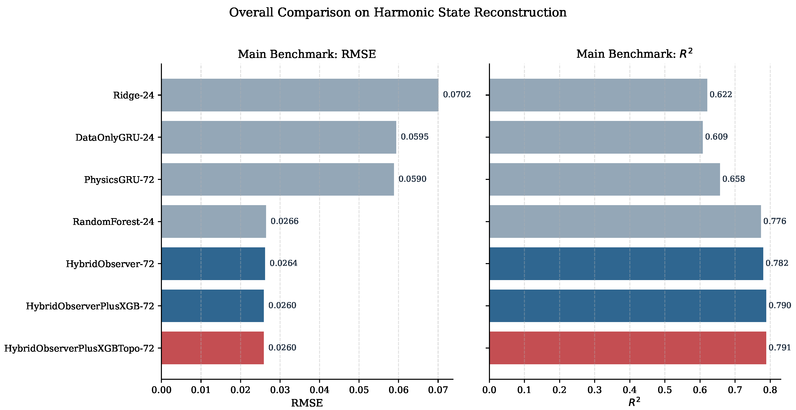
Table 2 compares the proposed method with representative traditional, deep-learning, and observer-style baselines. The final model, HybridObserverPlusXGBTopo-72, achieves the best overall result with R M S E 0.02604 , M A E 0.02054 , R 2 0.79060 , and  sMAPE = 0.01922 . In contrast, the strongest standard baseline is RandomForest-24, which yields RMSE = 0.02661 and R 2 = 0.77554 . This comparison highlights a central point of the paper: the proposed framework does not rely on replacing strong tabular learners, but on integrating them with observer-style branches so that statistical regularities, temporal dynamics, and topology-aware information are exploited jointly.
The ordering of the remaining baselines is also informative. Ridge regression provides a stable linear reference but is limited by the nonlinear nature of the problem. Random Forest and XGBoost are highly competitive, confirming that harmonic reconstruction in this dataset contains substantial structured nonlinear regularities. Pure sequence models such as LSTM, TCN, and DataOnlyGRU capture temporal behavior, but their standalone accuracy remains below that of the strongest ensemble baselines. Physics-guided observer models then bridge this gap and become especially valuable when used as complementary components in the final hybrid stack.
Figure 2 provides a highly intuitive visual stratification of the main benchmark, distinctly separating the evaluated models into three performance tiers. At the top of the charts (highest RMSE, lowest R 2 ), linear models and pure sequence networks (Ridge-24, DataOnlyGRU-24) struggle to establish a robust mapping, highlighting the severe limitations of unconstrained neural networks on highly non-stationary SCADA data. In the middle tier, the injection of physical domain knowledge (PhysicsGRU-72) clearly pushes the neural performance forward, reducing RMSE and improving R 2 compared to its data-only counterpart. However, the most significant error reduction is observed when transitioning to the hybrid architectures. The bottom cluster of bars visually confirms that once the physics-guided observer is fused with statistical tabular learners, the reconstruction error decreases substantially. Furthermore, the incremental extensions within the hybrid family, from HybridObserver-72 to the final HybridObserverPlusXGBTopo-72, demonstrate a consistent, monotonic improvement. This indicates that that integrating extreme gradient boosting and spatial topological priors provides the crucial final calibration, effectively squeezing out the residual errors to achieve the global optimum under both metrics simultaneously.

4.3.2. Per-Target and Multi-Window Analysis

Per-Target Resolution and Multi-Window Dynamics. To explicitly decipher the precise origins of the global performance gains, Table 3 dissects the reconstruction accuracy across the four specific harmonic target dimensions. A critical observation is that the proposed topological framework yields simultaneous, strictly monotonic improvements across all electrical variables. This confirms that the model avoids the “negative transfer” phenomenon commonly observed in multi-output regressions, where optimizing one target inadvertently degrades another.
Most remarkably, the predictive fidelity for the PCC-side voltage distortion ( T H D V 60 ) experiences a notable improvement, with  R 2 increasing from 0.44362 (using the RF-24 baseline) to 0.48581 . In an operational offshore context, the  60 kV PCC node serves as the aggregate integration point linking the entire wind farm to the external main grid. Its harmonic behavior is notoriously volatile and difficult to model due to compounded aerodynamic wake effects, transmission cable resonances, and background grid fluctuations. The significant accuracy boost at this specific node emphasizes the immense practical value of utilizing cross-node spatial priors to stabilize highly aggregated predictions. Stable, albeit smaller, improvements are also observed on T H D I 60 , T H D V 575 , and  T H D I 575 , culminating in an optimized multi-output reconstruction balance. Furthermore, the comparison across window lengths reveals that while a 24-h input is sufficient for memory-less tabular learners to extract immediate statistical snapshots, the physics-guided observer requires the expansive 72 h context to accurately deduce multi-scale temporal inertia and slow-moving meteorological trends.
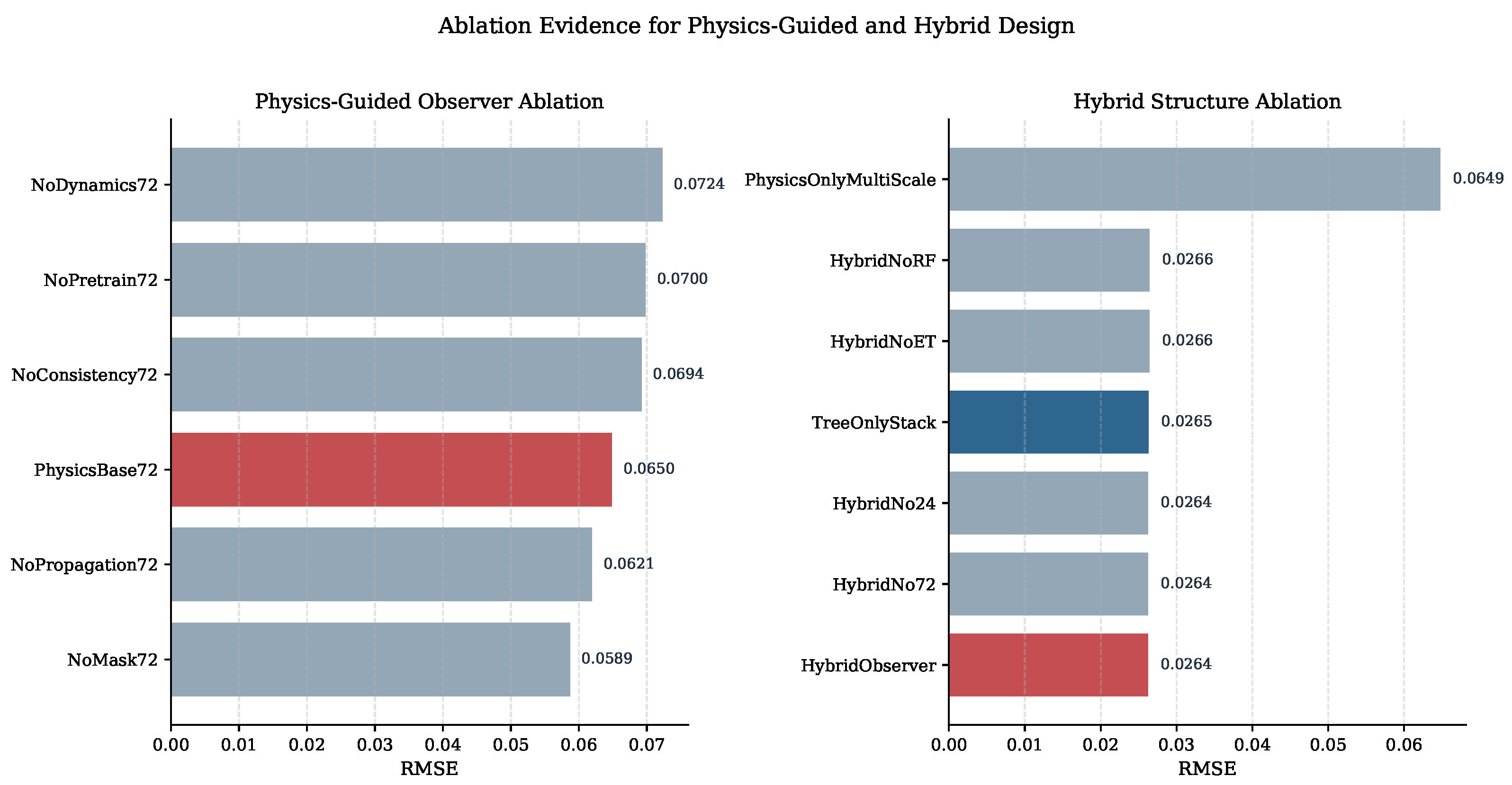
Visualizing the Ablation Mechanisms: Figure 3 complements the quantitative tables by providing a highly intuitive visual stratification of the ablation evidence. The left panel, detailing the Physics-Guided Observer Ablation, vividly illustrates the penalizing effect of removing domain knowledge. The topmost bars, particularly NoDynamics72 ( RMSE = 0.0724 ) and NoConsistency72 ( RMSE = 0.0694 ), demonstrate severe error inflation compared to the fully constrained PhysicsBase72. This visually corroborates that offshore electrical networks possess strong electromagnetic inertia; permitting the neural hidden states to fluctuate without differential dynamic penalization or absolute amplitude scaling inevitably leads to severe high-frequency tracking errors.
Conversely, the right panel, illustrating the Hybrid Structure Ablation, exposes the absolute necessity of the stacked fusion strategy. The standalone PhysicsOnlyMultiScale variant exhibits a massive performance gap ( RMSE = 0.0649 ) compared to the hybrid cluster at the bottom ( RMSE 0.0264 ). This explicitly refutes the assumption that deep physical networks alone can universally dominate complex power system modeling under data sparsity. Instead, it validates the proposed synergy: the final, narrow performance gains among the hybrid variants prove that baseline non-stationary tracking is best handled by tree models (TreeOnlyStack), thereby freeing the neural observer to focus entirely on injecting physical propagation priors and structural regularization. Together, these two panels visually prove that the global optimum is uniquely achieved by preserving both rigorous physical constraints and the hybrid fusion architecture.

4.3.3. Computational and Structural Efficiency

The proposed framework is also attractive from an implementation perspective. Rather than constructing a single monolithic network for all predictive mechanisms, the final method combines three practically efficient ingredients: strong tabular regressors, compact observer branches, and a lightweight positive linear fusion stage. This modular design yields two advantages. Specifically, each branch can be optimized with a training strategy suitable for its own inductive bias. AND the final fusion layer only operates on branch outputs instead of high-dimensional raw sequences, which keeps the last-stage optimization simple and stable.
This structural efficiency is important for offshore harmonic monitoring. In practice, a deployable solution must balance predictive quality with engineering manageability. The proposed hybrid formulation achieves this balance by preserving the statistical strength of tree-based methods while adding observer branches only where they contribute complementary temporal and topology-aware information.

4.4. Performance Analysis of Physics-Guided and Topology-Aware Design

Physics/Topology Ablation

Table 4 reports the internal ablation results for the 72 h physics-guided observer branch. Three components stand out as especially beneficial.
Specifically, the consistency term is important for maintaining coherence between the auxiliary harmonic proxy and the final reconstructed state. Removing it increases RMSE from 0.06505 to 0.06939 . Then, latent dynamics regularization contributes strongly to temporal stability; removing this term leads to the largest degradation, with RMSE rising to 0.07245 . Moreover, masked pretraining improves the observer representation before supervised fine-tuning, and removing it similarly degrades performance to 0.06998 .
The masking term deserves separate attention. When the objective is the main reconstruction score alone, the NoMask72 variant achieves the lowest RMSE among the ablated observer variants. However, this should be interpreted as a task specialization effect rather than a contradiction: the masking mechanism is designed to prepare the observer for partial observability and therefore becomes most valuable in cross-node virtual sensing. In other words, the main-task optimum and the observability-oriented optimum need not coincide, and the proposed framework is deliberately designed to support both.
Moreover, the NoPropagation72 result indicates that the strongest and most stable gains currently come from consistency, dynamics, and masked pretraining. The propagation prior remains meaningful as a topology-oriented inductive bias, but its benefits are expressed more clearly in cross-node tasks than in the main RMSE metric alone.
Hybrid Structure Ablation: Table 5 explicitly quantifies the contribution of the observer-style fusion architecture. While the standalone TreeOnlyStack establishes a highly competitive baseline ( RMSE = 0.02646 , R 2 = 0.77988 ), the fully integrated HybridObserver successfully breaches this performance ceiling ( RMSE = 0.02640 , R 2 = 0.78083 ). This numerically confirms that the physics-guided observer branches inject complementary dynamic inertia that static tabular learners structurally cannot extract.
Furthermore, ablating specific temporal scales (HybridNo24, HybridNo72) or individual tree ensembles (HybridNoET, HybridNoRF) triggers measurable, albeit graceful, performance degradations. For instance, excising the Random Forest branch notably degrades the R 2 to 0.77626 . This indicates that while the ensemble components are partially redundant, their collective diversity is crucial for maximizing generalization stability.
Most critically, the PhysicsOnlyMultiScale variant completely fails to generalize effectively in isolation, exhibiting a substantial error increase (RMSE = 0.06492, R 2 = 0.63985). Conversely, the TreeOnlyStack establishes a strong statistical baseline but fundamentally lacks physical memory. This stark contrast clearly demonstrates that the final state-of-the-art performance is strictly born from their principled complementarity: robust tree ensembles (like XGBoost) handle the “heavy lifting” of the highly non-stationary statistical mapping, while the PINN-inspired neural observer contributes by enforcing smooth physical transitions and correcting unphysical residuals. The measurable improvement from TreeOnlyStack to the fully integrated HybridObserver mathematically isolates the unique value of embedding physical inertia into the regression pipeline.

4.5. Cross-Node Virtual Sensing Analysis

4.5.1. Experimental Setup for Virtual Sensing

To evaluate whether the proposed framework captures cross-node coupling rather than only direct pointwise reconstruction, we conduct virtual sensing experiments under partial observation. Two masking scenarios are considered: S 1 = Hide _ B 60 and S 2 = Hide _ B 575 . In each scenario, the corresponding node group is hidden from the input, and the model reconstructs the missing harmonic state using the remaining observations. This setting closely matches the intended engineering use case of observer-assisted harmonic monitoring under incomplete sensor coverage.

4.5.2. Comparative Results

The comparative results are listed in Table 6. Two strong observations emerge. Specifically, the two scenarios differ substantially in difficulty. Reconstructing the hidden WT-side node B 575 is much easier than reconstructing the hidden PCC-side node B 60 . Second, the strongest model depends on the scenario. PhysicsGRU-72 achieves the best result on Hide_B575, while ContinuousPhysicsObserver-24 performs best on the more challenging Hide_B60 task. This pattern shows that topology-aware observer modeling contributes most visibly when direct measurements are missing and the model must infer harmonic states from node coupling structure.
Furthermore, these virtual sensing results explicitly isolate the qualitative contribution of the PINN-inspired architecture. While ensemble methods like XGBoost provide excellent pointwise accuracy under full observability, they structurally lack the capability to infer states across spatial graphs when sensors are disabled. The topology-aware observer overcomes this limitation by actively leveraging the mathematical coupling structures (e.g., the graph Laplacian) and physical propagation priors, thereby granting the system a critical cross-node virtual sensing capability that pure statistical baselines cannot achieve.

4.6. Robustness and Generalization Analysis

4.6.1. Noise Robustness

To examine robustness under input perturbation, Gaussian noise is added to the best physics-guided observer input:
X ˜ t ( L ) = X t ( L ) + ξ t , ξ t N ( 0 , σ n 2 I ) ,
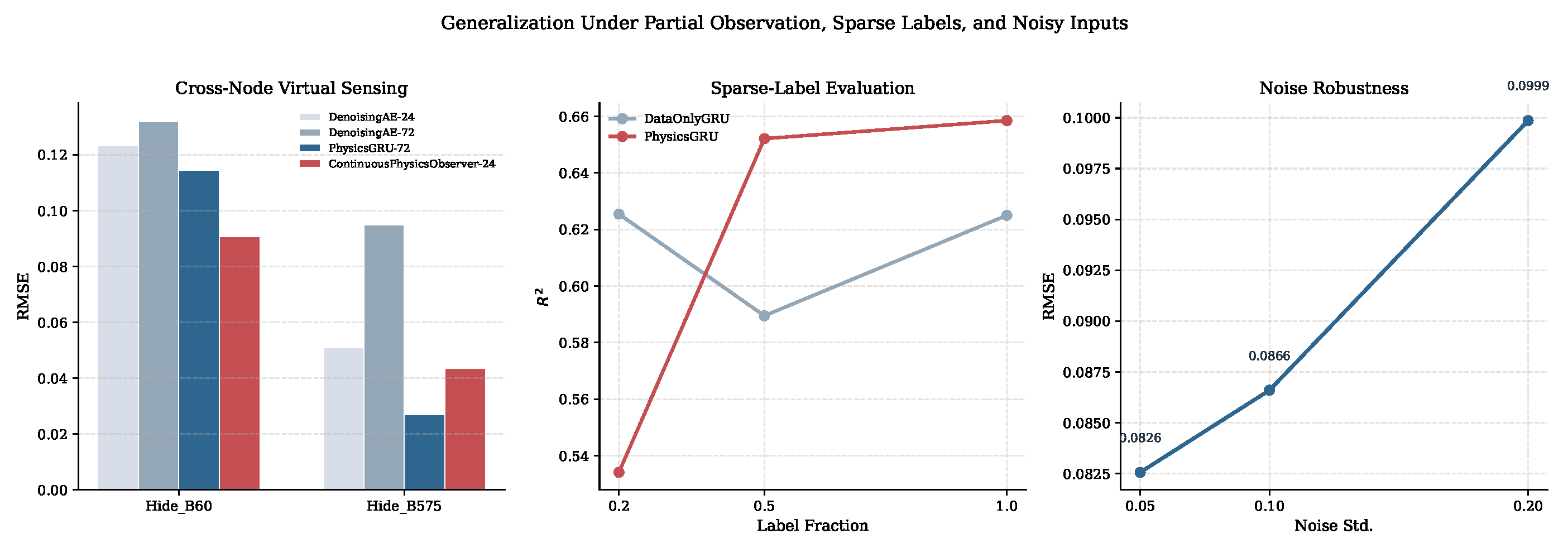
where the noise standard deviation takes values 0.05, 0.10, and 0.20. The resulting reconstruction errors under these respective noise levels are RMSE 0.05 = 0.08256 , RMSE 0.10 = 0.08660 , and  RMSE 0.20 = 0.09986 . This smooth degradation pattern indicates that the observer remains functional under moderate disturbance and preserves a stable ranking of prediction quality as noise increases. For practical offshore operations, such graceful degradation is highly valuable because measurement perturbations and communication noise are difficult to avoid completely.

4.6.2. Sparse-Label Evaluation

We also evaluate the effect of reduced supervision by randomly retaining part of the training labels. The label-retention ratios are set to 0.2, 0.5, and 1.0.
Table 7 compares the sparse-label DataOnlyGRU and PhysicsGRU models. Under moderate and full supervision, corresponding to label fractions 0.5 and 1.0, the physics-guided model achieves the better result, showing that the proposed regularization strategy remains beneficial once a reasonable amount of supervision is available. Under the most aggressive setting, with label fraction 0.2, the data-only branch retains a slight advantage, while the physics-guided model remains competitive. This overall pattern is encouraging: the proposed framework becomes increasingly favorable as more supervision is available, while still remaining viable in lower-label regimes.

4.6.3. Continuous-Time Extension

Because the original framework motivation also included continuous-time observer design, we further evaluate whether the continuous branch can complement the strongest discrete model on the subset of timestamps shared by both formulations:
T a l i g n = T d i s c T c o n t .
Continuous-Time Extension and Sample Alignment: Because the original framework motivation also encompasses continuous-time observer design, we further evaluate whether the continuous branch can complement the strongest discrete model on the specific subset of timestamps shared by both formulations ( T a l i g n = T d i s c T c o n t ). On this strictly aligned subset (comprising 1755 validation and 1759 test samples), the enhanced configuration AlignedBestDiscretePlusCP72 reaches RMSE = 0.02602 , MAE = 0.02053 , and  R 2 = 0.79054 . Although this result is reported on a specialized subset rather than the full official benchmark, it successfully proves that explicitly modeling continuous-time dynamics provides complementary feature representations, capable of marginally refining the predictions of an already highly optimized discrete stack.
Visualizing Generalization and Observability: Figure 4 visually summarizes the framework’s overarching resilience under extreme, non-ideal operating conditions, acting as a comprehensive robustness evaluation for the proposed architecture. The figure is strategically divided into three operational challenges. Specifically, the left panel (Cross-Node Virtual Sensing) vividly illustrates the disparity in spatial reconstruction difficulty. The standard data-driven imputation baseline (DenoisingAE) struggles significantly across both scenarios. Crucially, the ContinuousPhysicsObserver-24 (red bar) unequivocally dominates the highly challenging Hide_B60 task. This visually corroborates that when inferring the aggregated PCC-side harmonics from isolated turbine data, a severely ill-posed inverse problem, explicitly modeling temporal gaps and physical propagation paths is highly beneficial.
Then, the middle panel (Sparse-Label Evaluation) reveals a divergent performance trend under varying supervision levels. The physics-guided model (red line) exhibits exceptional scalability, dominating the naive DataOnlyGRU (grey line) under moderate (0.5) to full (1.0) supervision. However, the sharp drop of the red line at the 0.2 label fraction uncovers a fundamental characteristic of PINN-inspired architectures: physical and topological constraints require a “critical mass” of ground-truth boundary conditions to correctly establish the underlying differential manifold. Below this threshold, pure data-driven mapping temporarily survives better, though at a strictly suboptimal R 2 ceiling.
Moreover, the right panel (Noise Robustness) explicitly tracks the RMSE trajectory under increasing additive sensor noise. Rather than exhibiting an exponential explosion or catastrophic divergence, the error climbs in a smooth, nearly linear progression (from 0.0826 to 0.0999 ). This graceful degradation empirically verifies the regularizing effect of the physical constraints, which effectively anchor the neural predictions and prevent the model from indiscriminately fitting to high-frequency stochastic noise. For practical offshore operations, this guarantees that diagnostic early-warning systems remain trustworthy despite inevitable communication latency and sensor drift.

5. Conclusions

To address the critical challenge of dynamic harmonic state reconstruction in complex, partially observable offshore wind farms, this paper proposes a novel PINN-inspired topology-aware learning framework. Moving beyond purely data-driven black-box models and rigid, intractable physical equation solvers, the proposed method innovatively embeds physical consistency constraints, latent dynamic regularizations, and asymmetric topological priors into a temporal sequence observer. By employing an observer-style hybrid fusion strategy via non-negative stacked generalization, the framework seamlessly integrates the sequential memory capabilities of deep recurrent networks with the statistical robustness of tree-based tabular learners. Extensive evaluations using real-world multi-node coupled system data confirm the superiority of the proposed framework. Furthermore, rigorous spatial masking experiments validate the framework’s cross-node virtual sensing capabilities, demonstrating stable and high-fidelity harmonic state reconstruction even for physically unmonitored turbines. Ultimately, this research bridges the gap between physics-informed learning and data-driven state estimation. It provides a highly resilient, practically deployable paradigm for ubiquitous harmonic monitoring and proactive risk mitigation in modern inverter-based power grids under severely restricted measurement conditions.

Author Contributions

Methodology, X.Z. and L.Z.; validation, Q.C.; Formal analysis, Q.W. and N.Z.; Investigation, X.Z., L.Z. and Q.C.; Writing—original draft, X.Z., L.Z. and Q.C.; Writing—review & editing, X.Z., L.Z., J.P. and Y.Z.; Supervision, Q.W. and N.Z. All authors have read and agreed to the published version of the manuscript.

Funding

This work was supported in part by China Southern Power Grid Co., Ltd. Science and Technology Project under Grant No. YNKJXM20240262.

Data Availability Statement

To ensure the scientific transparency and reproducibility of this research, the complete executable source code of the proposed PINN-inspired topology-aware learning framework, along with a sampled “dummy” dataset for structural verification, has been made publicly available at: https://github.com/forlexa/PINN-data?tab=readme-ov-file, accessed on 14 May 2026. The original real-world Turkish wind meteorological dataset used to drive the electrical simulations can be accessed via its respective public repository.

Conflicts of Interest

Authors Xin Zhou, Li Zhang, Junzhen Peng and Yongshuai Zhao were employed by Electric Power Institute, Yunnan Power Grid Company Ltd. The remaining authors declare that the research was conducted in the absence of any commercial or financial relationships that could be construed as a potential conflict of interest. The authors declare that this study received funding from Electric Power Institute, Yunnan Power Grid Company Ltd. The funder had the following involvement with the study: Methodology, validation, Investigation, Writing—original draft, Writing—review & editing.

References

  1. Hatziargyriou, N.; Milanovic, J.; Rahmann, C.; Ajjarapu, V.; Canizares, C.; Erlich, I.; Hill, D.; Hiskens, I.; Kamwa, I.; Pal, B.; et al. Definition and Classification of Power System Stability–Revisited & Extended. IEEE Trans. Power Syst. 2021, 36, 3271–3281. [Google Scholar]
  2. Wang, X.; Blaabjerg, F. Harmonic Stability in Power Electronic-Based Power Systems: Concept, Modeling, and Analysis. IEEE Trans. Smart Grid 2019, 10, 2858–2870. [Google Scholar] [CrossRef]
  3. Chen, Q.; Bu, S. Impedance-Based Stability Analysis of Power System Wideband Oscillations: A Bridge between s Domain and Frequency Domain. IEEE Trans. Power Syst. 2024, 39, 5854–5868. [Google Scholar] [CrossRef]
  4. Huang, X.; Huang, H.; Pan, X.; Xu, Q.; He, B.; Zhang, Z.; Xu, Z. Harmonic Resonance Mode Analysis for Offshore Wind Power System Based on Impedance Gathering. In Proceedings of the 2024 IEEE PES 16th Asia-Pacific Power and Energy Engineering Conference (APPEEC), Nanjing, China, 25–27 October 2024; IEEE: New York, NY, USA, 2024; pp. 1–5. [Google Scholar]
  5. Wang, M.; Hernandez Manchola, A.J.; Raab, A.; Mehlmann, G.; Luther, M. Power Oscillation Damping from VSC-HVDC Connected Offshore Wind Farms using DC Link Braking Chopper. In Proceedings of the 2023 25th European Conference on Power Electronics and Applications (EPE’23 ECCE Europe), Aalborg, Denmark, 4–8 September 2023; IEEE: New York, NY, USA, 2023; pp. 1–8. [Google Scholar]
  6. de Souza, L.A.A.; Martins, M.B.; Pinto, M.V.V.; Lima, A.C.S.; Moura Junior, N.N. Data-Driven Modeling of Nonlinear Transducers for Harmonic Measurements. IEEE Trans. Instrum. Meas. 2025, 74, 1–8. [Google Scholar] [CrossRef]
  7. Wang, Z.; Ma, Z.; Yu, S.; Wu, M.; Gao, J. Mechanism of Broadband Harmonic Amplification and Insulation Deterioration in DC Submarine Cables. In Proceedings of the 2024 IEEE PES 16th Asia-Pacific Power and Energy Engineering Conference (APPEEC), Nanjing, China, 25–27 October 2024; IEEE: New York, NY, USA, 2024; pp. 1–5. [Google Scholar]
  8. Du, B.; Narusue, Y.; Furusawa, Y.; Nishihara, N.; Indo, K.; Morikawa, H.; Iida, M. Clustering Wind Turbines for SCADA Data-Based Fault Detection. IEEE Trans. Sustain. Energy 2023, 14, 442–452. [Google Scholar] [CrossRef]
  9. Alimi, O.A.; Ouahada, K.; Abu-Mahfouz, A.M. A Review of Machine Learning Approaches to Power System Security and Stability. IEEE Access 2020, 8, 113512–113531. [Google Scholar] [CrossRef]
  10. Wang, J.; Li, Z.; Lai, P.; Wang, R.; Yang, D.; Yang, D.; Xu, H.; Tao, W.Q. A Novel Paradigm in Solving Multiscale Problems. arXiv 2024, arXiv:2402.05067. [Google Scholar] [CrossRef]
  11. Falas, S.; Asprou, M.; Konstantinou, C.; Michael, M.K. Robust Power System State Estimation Using Physics-Informed Neural Networks. IEEE Trans. Ind. Inform. 2025, 21, 8057–8067. [Google Scholar] [CrossRef]
  12. Siqueira-de Carvalho, R.; Morales-Paredes, H.K.; Bates, C.; Ausmus, J.; Simões, M.G.; Sen, P.K. Overview of Big Data Analytics in Power Quality Analysis and Assessment. In Proceedings of the 9th Brazilian Technology Symposium (BTSym’23); Springer: Cham, Switzerland, 2024; pp. 3–16. [Google Scholar]
  13. Ullah, M.; Guan, Y.; Yu, Y.; Chaudhary, S.K.; Vasquez, J.C.; Guerrero, J.M. Dynamic Performance and Power Quality of Large-Scale Wind Power Plants: A Review on Challenges, Evolving Grid Code, and Proposed Solutions. IEEE Open J. Power Electron. 2025, 6, 1148–1173. [Google Scholar] [CrossRef]
  14. GWEC. Global Wind Report 2024; Global Wind Energy Council: Brussels, Belgium, 2024. [Google Scholar]
  15. IRENA. World Energy Transitions Outlook 2024; International Renewable Energy Agency: Abu Dhabi, United Arab Emirates, 2024. [Google Scholar]
  16. Tang, Z.; Yang, Y.; Blaabjerg, F. Power electronics: The enabling technology for renewable energy integration. CSEE J. Power Energy Syst. 2022, 8, 39–52. [Google Scholar]
  17. Wang, Y.; Ma, H.; Xiao, X.; Wang, Y.; Zhang, Y.; Wang, H. Harmonic State Estimation for Distribution Networks Based on Multi-Measurement Data. IEEE Trans. Power Deliv. 2023, 38, 2311–2325. [Google Scholar] [CrossRef]
  18. Li, G.Y.; Yen, H.J.; Wu, J.W.; Huang, W.Y.; Chang, G.W. A Comparative Study of Harmonic Distortion Assessment for an Offshore Wind Farm System. In Proceedings of the 2024 21st International Conference on Harmonics and Quality of Power (ICHQP), Chengdu, China, 15–18 October 2024; IEEE: New York, NY, USA, 2024; pp. 451–456. [Google Scholar]
  19. IEEE 519-2022; IEEE Standard for Harmonic Control in Electric Power Systems. IEEE: New York, NY, USA, 2022; pp. 1–31.
  20. IEC/TR 61000-3-6; Electromagnetic Compatibility (EMC)—Part 3–6: Limits-Assessment of Emission Limits for the Connection of Distorting Installations to MV, HV and EHV Power Systems. IEC: Geneva, Switzerland, 2008.
  21. Huang, H.; Lin, L.; Xu, Q.; He, B.; Zhang, Z.; Ye, Q. Offshore Wind Power System Resonance Stability: Modelling, Analysis, and Methods Comparison. In Proceedings of the 2025 10th Asia Conference on Power and Electrical Engineering (ACPEE); IEEE: New York, NY, USA, 2025; pp. 1464–1472. [Google Scholar]
  22. Lakshmanan, P.; Sun, R.; Liang, J. Electrical collection systems for offshore wind farms: A review. CSEE J. Power Energy Syst. 2021, 7, 1078–1092. [Google Scholar] [CrossRef]
  23. Hou, P.; Zhu, J.; Ma, K.; Yang, G.; Hu, W.; Chen, Z. A review of offshore wind farm layout optimization and electrical system design methods. J. Mod. Power Syst. Clean Energy 2019, 7, 975–986. [Google Scholar] [CrossRef]
  24. Ji, X.; Xu, H.; Liu, H.; Kong, X. Modeling and Stability Analysis of DFIG-Based Wind Farm Using Harmonic State Space Theory. In Proceedings of the 2025 Zhejiang Power Electronics Conference (ZPEC), Hangzhou, China, 23–24 August 2025; IEEE: New York, NY, USA, 2025; pp. 232–237. [Google Scholar]
  25. Zhang, Y.; Klabunde, C.; Wolter, M. Frequency-Coupled Impedance Modeling and Resonance Analysis of DFIG-Based Offshore Wind Farm With HVDC Connection. IEEE Access 2020, 8, 147880–147894. [Google Scholar] [CrossRef]
  26. Lim, B.; Zohren, S. Time-series forecasting with deep learning: A survey. Philos. Trans. R. Soc. A Math. Phys. Eng. Sci. 2021, 379, 20200209. [Google Scholar] [CrossRef] [PubMed]
  27. Hochreiter, S.; Schmidhuber, J. Long Short-Term Memory. Neural Comput. 1997, 9, 1735–1780. [Google Scholar] [CrossRef]
  28. Elymany, M.M.; Enany, M.A.; Elsonbaty, N.A. Hybrid optimized-ANFIS based MPPT for hybrid microgrid using zebra optimization algorithm and artificial gorilla troops optimizer. Energy Convers. Manag. 2024, 299, 117809. [Google Scholar] [CrossRef]
  29. Hadi, F.M.A.; Aly, H.H.; Little, T. Harmonics Forecasting of Wind and Solar Hybrid Model Based on Deep Machine Learning. IEEE Access 2023, 11, 100438–100457. [Google Scholar] [CrossRef]
  30. Vaswani, A.; Shazeer, N.; Parmar, N.; Uszkoreit, J.; Jones, L.; Gomez, A.N.; Kaiser, L.; Polosukhin, I. Attention is all you need. In Proceedings of the 31st International Conference on Neural Information Processing Systems, Long Beach, CA, USA, 4–9 December 2017; pp. 6000–6010. [Google Scholar]
  31. Wu, H.; Xu, J.; Wang, J.; Long, M. Autoformer: Decomposition Transformers with Auto-Correlation for Long-Term Series Forecasting. In Proceedings of the Advances in Neural Information Processing Systems; Beygelzimer, A., Dauphin, Y., Liang, P., Vaughan, J.W., Eds.; Curran Associates Inc.: Red Hook, NY, USA, 2021. [Google Scholar]
  32. Hadi, F.M.A.; Aly, H.H.; Little, T. Harmonics Forecasting of Wind and Solar Hybrid Model Driven by DFIG and PMSG Using ANN and ANFIS. IEEE Access 2023, 11, 55413–55424. [Google Scholar] [CrossRef]
  33. Lin, J.; Tu, M.; Hong, H.; Lu, C.; Song, W. Spatiotemporal Graph Convolutional Neural Network-Based Forecasting-Aided State Estimation Using Synchrophasors. IEEE Internet Things J. 2024, 11, 16171–16183. [Google Scholar] [CrossRef]
  34. Iqbal, M.A.; Ahn, J.; Kim, S.K. Spatio-Temporal Hybrid Graph-Transformer Model for High-Fidelity Renewable Energy Forecasting. J. Mod. Power Syst. Clean Energy 2026, 1–12. [Google Scholar] [CrossRef]
  35. Luo, X.; Zhang, D.; Zhu, X. Deep learning based forecasting of photovoltaic power generation by incorporating domain knowledge. Energy 2021, 225, 120240. [Google Scholar] [CrossRef]
  36. Hyde, D.; Kadapa, C.; Albustami, A.A.; Taha, A.F. Progress and Perils of PINNs: Perspectives on Applying Physics-Informed Neural Networks to Science and Engineering Problems. Comput. Sci. Eng. 2026, 1–9. [Google Scholar] [CrossRef]
  37. Breiman, L. Random Forests. Mach. Learn. 2001, 45, 5–32. [Google Scholar] [CrossRef]
  38. Liu, Y.; Luo, H.; Zhao, B.; Zhao, X.; Han, Z. Short-Term Power Load Forecasting Based on Clustering and XGBoost Method. In Proceedings of the 2018 IEEE 9th International Conference on Software Engineering and Service Science (ICSESS), Beijing, China, 23–25 November 2018; IEEE: New York, NY, USA, 2018; pp. 536–539. [Google Scholar]
  39. Hao, C.; Chu, J.; Han, T.; Hu, Q. Partial Discharge Recognition of Medium Voltage Switchgear Based on CatBoost Model. In Proceedings of the 2024 IEEE 5th International Conference on Dielectrics (ICD), Toulouse, France, 30 June–4 July 2024; IEEE: New York, NY, USA, 2024; pp. 1–4. [Google Scholar]
  40. Liu, R. Research on LightGBM Algorithm for Subway Gate Fault Detection. In Proceedings of the 2024 International Conference on Control, Electronic Engineering and Machine Learning (CEEML), Kuala Lumpur, Malaysia, 22–24 November 2024; IEEE: New York, NY, USA, 2024; pp. 116–120. [Google Scholar]
  41. Karadeniz, A. Advancing harmonic prediction for offshore wind farms using synthetic data and machine learning. Comput. Electr. Eng. 2025, 127, 110613. [Google Scholar] [CrossRef]
  42. An, H.; Ma, J. Fast diffusion-driven data augmentation for imbalanced power-system stability classification. Int. J. Electr. Power Energy Syst. 2026, 175, 111559. [Google Scholar] [CrossRef]
  43. Yang, S.; Xiao, W.; Zhang, M.; Guo, S.; Zhao, J.; Shen, F. Image Data Augmentation for Deep Learning: A Survey. arXiv 2023, arXiv:2204.08610. [Google Scholar] [CrossRef]
  44. MilovanoviC, M.; RadosavljeviC, J.; PeroviC, B. A backward/forward sweep power flow method for harmonic polluted radial distribution systems with distributed generation units. Int. Trans. Electr. Energy Syst. 2020, 30, e12310. [Google Scholar] [CrossRef]
  45. Milovanović, M.; Radosavljević, J.; Perović, B.; Dragičević, M. Power flow in radial distribution systems in the presence of harmonics. Int. J. Electr. Eng. Comput. 2018, 2, 11–19. [Google Scholar] [CrossRef]
  46. Cho, K.; Van Merriënboer, B.; Gulcehre, C.; Bahdanau, D.; Bougares, F.; Schwenk, H.; Bengio, Y. Learning phrase representations using RNN encoder-decoder for statistical machine translation. arXiv 2014, arXiv:1406.1078. [Google Scholar] [CrossRef]
  47. Huber, P.J. Robust estimation of a location parameter. Ann. Math. Stat. 1964, 35, 73–101. [Google Scholar] [CrossRef]
  48. Wolpert, D.H. Stacked generalization. Neural Netw. 1992, 5, 241–259. [Google Scholar] [CrossRef]
  49. Chen, T.; Guestrin, C. XGBoost: A Scalable Tree Boosting System. In Proceedings of the 22nd ACM SIGKDD International Conference on Knowledge Discovery and Data Mining, San Francisco, CA, USA, 13–17 August 2016; Association for Computing Machinery: New York, NY, USA, 2016; pp. 785–794. [Google Scholar]
  50. Lawson, C.L.; Hanson, R.J. Solving Least Squares Problems; Prentice-Hall: Englewood Cliffs, NJ, USA, 1974. [Google Scholar]
  51. Bai, S.; Kolter, J.Z.; Koltun, V. An Empirical Evaluation of Generic Convolutional and Recurrent Networks for Sequence Modeling. arXiv 2018, arXiv:1803.01271. [Google Scholar] [CrossRef]
  52. Vincent, P.; Larochelle, H.; Lajoie, I.; Bengio, Y.; Manzagol, P. Stacked Denoising Autoencoders: Learning Useful Representations in a Deep Network with a Local Denoising Criterion. J. Mach. Learn. Res. 2010, 11, 3371–3408. [Google Scholar]
  53. Kadlec, P.; Gabrys, B.; Strandt, S. Data-driven Soft Sensors in the Process Industry. Comput. Chem. Eng. 2009, 33, 795–814. [Google Scholar] [CrossRef]
Figure 1. Schematic diagram of the PINN-inspired topology-aware learning framework for harmonic state recognition. By optimizing a joint objective function that combines empirical data loss with physics-informed regularization, the framework processes sparse grid measurement data to accurately estimate dynamic harmonic states within multi-node coupled systems.
Energies 19 02564 g001
Figure 2. Visual overview of the main benchmark. The proposed HybridObserverPlusXGBTopo-72 achieves the lowest RMSE and the highest R 2 among representative baselines and hybrid variants.
Energies 19 02564 g002
Figure 3. Visual summary of ablation results. (Left): RMSE changes for physics-guided observer ablations. (Right): RMSE changes for hybrid-structure ablations. Lower is better in both panels.
Energies 19 02564 g003
Figure 4. Generalization and observability analysis. (Left): cross-node virtual sensing RMSE under Hide_B60 and Hide_B575. (Middle): R 2 under sparse-label training. (Right): RMSE degradation under additive input noise.
Energies 19 02564 g004
Table 1. Nomenclature.
Abbreviations
        OWFOffshore Wind Farm
        WTGWind Turbine Generator
        PCCPoint of Common Coupling
        IBRInverter-Based Resource
        THDTotal Harmonic Distortion
        PINNPhysics-Informed Neural Network
        GRUGated Recurrent Unit
        LSTMLong Short-Term Memory
        TCNTemporal Convolutional Network
        RFRandom Forest
        XGBoosteXtreme Gradient Boosting
        NNLSNon-Negative Least Squares
        SCADASupervisory Control and Data Acquisition
        RMSERoot Mean Square Error
        MAEMean Absolute Error
        sMAPESymmetric Mean Absolute Percentage Error
Mathematical Symbols
         NTotal number of physical nodes
         G ( V , E , A ) Undirected weighted graph representing the network topology
         V Set of physical nodes
         E Set of submarine cable connections (edges)
         AWeighted adjacency matrix
         DDiagonal degree matrix
         LGraph Laplacian matrix
         hHarmonic order
         Y h Network admittance matrix at the h-th harmonic order
         V h , I h Vectors of nodal harmonic voltages and current injections
         x t Integrated feature vector at time step t
         X t ( L ) Sliding temporal observation window of length L
         y t , y ^ t Ground-truth and predicted dynamic harmonic state vectors
         c t Terminal hidden state aggregating sequential information
         e t , e ^ t Actual and predicted empirical harmonic proxy vectors
         M g Channel-masking operator for virtual sensing
         L o b s Total objective loss function for the observer
         β k Optimal weighting coefficients for hybrid fusion
Table 2. Main harmonic state reconstruction results on the test set.
ModelWindowRMSEMAE R 2 sMAPE
Ridge240.070220.054820.622070.03121
RandomForest240.026610.021050.775540.01998
XGBoost240.026940.021030.784460.01954
DataOnlyGRU240.059540.044260.609250.02843
LSTM240.057980.043260.662850.02824
TCN240.095800.074790.085830.03948
ContinuousPhysicsObserver240.066690.050390.527940.02981
PhysicsGRU720.058970.043890.658470.02825
HybridObserver720.026370.020840.781950.01969
HybridObserverPlusXGB720.026050.020550.790180.01923
HybridObserverPlusXGBTopo720.026040.020540.790600.01922
Table 3. Per-target comparison between the strongest standard baseline and the final proposed model.
TargetRF-24 RMSEOurs RMSERF-24 R 2 Ours R 2
THDV600.029050.027930.443620.48581
THDI600.033780.033570.981920.98215
THDV5750.013130.012760.678800.69656
THDI5750.030490.029890.997810.99789
Table 4. Ablation results for the 72 h physics-guided observer branch.
VariantRMSEMAE R 2 sMAPE
PhysicsBase720.065050.048810.620850.02962
NoConsistency720.069390.053090.535830.03196
NoPropagation720.062120.046150.630950.02881
NoDynamics720.072450.056180.467610.03322
NoMask720.058870.043700.642960.02850
NoPretrain720.069980.053990.517540.03318
Table 5. Hybrid-structure ablation results.
VariantRMSEMAE R 2 sMAPE
HybridObserver0.026400.020860.780830.01970
TreeOnlyStack0.026460.020900.779880.01974
HybridNo240.026420.020880.780880.01970
HybridNo720.026410.020930.776010.01992
HybridNoET0.026560.020930.780660.01973
HybridNoRF0.026580.021040.776260.01998
PhysicsOnlyMultiScale0.064920.048040.639850.02919
Table 6. Cross-node virtual sensing results. Lower is better.
ScenarioModelRMSEMAE
Hide_B60DenoisingAE-240.123270.09579
Hide_B60DenoisingAE-720.131930.10461
Hide_B60PhysicsGRU-720.114460.06901
Hide_B60ContinuousPhysicsObserver-240.090610.06661
Hide_B575DenoisingAE-240.051020.04008
Hide_B575DenoisingAE-720.094900.07063
Hide_B575ContinuousPhysicsObserver-240.043540.03453
Hide_B575PhysicsGRU-720.027000.01959
Table 7. Sparse-label performance.
Label FractionModelRMSEMAE R 2
0.2SparseDataOnlyGRU0.061980.047070.62542
0.2SparsePhysicsGRU0.064270.048120.53413
0.5SparseDataOnlyGRU0.062910.047160.58949
0.5SparsePhysicsGRU0.060040.044600.65209
1.0SparseDataOnlyGRU0.060340.044710.62498
1.0SparsePhysicsGRU0.058970.043890.65847
Disclaimer/Publisher’s Note: The statements, opinions and data contained in all publications are solely those of the individual author(s) and contributor(s) and not of MDPI and/or the editor(s). MDPI and/or the editor(s) disclaim responsibility for any injury to people or property resulting from any ideas, methods, instructions or products referred to in the content.