Degradation-Aware Stochastic Scheduling of Multi-Stack Power-to-X Plants Under Joint Renewable and Electricity Price Uncertainty

Abstract

The day-ahead scheduling of multi-stack Power-to-X (PtX) plants must simultaneously cope with stack degradation under variable loading and with compound uncertainty in renewable generation and electricity prices. Existing scheduling frameworks address these two challenges in isolation, since degradation-aware models remain deterministic and stochastic models treat the electrolyser as a constant-efficiency device. This work develops a degradation-aware two-stage stochastic mixed-integer linear programming (MILP) framework that closes this gap. First-stage binaries fix the commitment and startup decisions of every stack, while second-stage scenario-indexed variables capture the dispatch, the hydrogen output, the shortfall, and the load-dependent and start–stop cycling degradation cost monetised at the stack level through a piecewise linear epigraph. Joint wind price uncertainty is represented by a Gaussian copula fitted on empirical CDF marginals and reduced to twenty representative scenarios via k-medoids clustering. The framework is fully implemented in MATLAB R2024a with the Optimization Toolbox, using the built-in intlinprog and linprog solvers. On a 100 MW reference plant with ten heterogeneous PEM stacks, out-of-sample evaluation against four formal benchmarks demonstrates the lowest LCOH at EUR 24/kg, the highest demand reliability at 85.0%, the highest hydrogen delivery at 7.68 t/day, and up to 50% total cost reduction over deterministic baselines, with end-to-end runtime under two minutes on standard workstation hardware.

1. Introduction

1.1. Power-to-X and the Role of Electrolyser-Based Hydrogen Production

The accelerating decarbonization of power, heat, transport and chemical sectors has positioned Power-to-X (PtX) technologies at the core of global energy transition strategies [1,2,3]. By converting surplus renewable electricity into hydrogen and downstream derivatives such as ammonia, methanol and synthetic fuels, PtX pathways provide long-duration storage, sector coupling and a credible route for decarbonizing hard-to-electrify industries [1,4]. Within this landscape, water electrolysis constitutes the indispensable backbone of the entire PtX value chain [5,6], and its techno-economic and operational performance directly governs the levelised cost of hydrogen (LCOH) and, hence, the viability of PtX deployment at industrial scale [7,8].

Although single-unit electrolysers have matured rapidly, achieving the multi-gigawatt capacities announced worldwide requires the aggregation of dozens to hundreds of stacks into multi-stack PtX plants [9,10]. The operation of such fleets is fundamentally different from that of a single unit: stacks are heterogeneous in health state, response dynamics and efficiency, and must be coordinated under variable renewable input and volatile electricity markets [11,12,13]. Optimal scheduling of multi-stack electrolyser fleets has therefore emerged as a central research problem at the intersection of process systems engineering, power systems optimization and chemical engineering [1,5,14].

1.2. The Degradation–Flexibility Trade-Off

A key but still poorly integrated aspect of electrolyser operation is performance degradation under variable loading. Experimental campaigns on both proton-exchange-membrane (PEM) and alkaline technologies have demonstrated that dynamic operation, frequent start–stop events and extended idling accelerate catalyst dissolution, membrane thinning and ohmic-resistance growth, thereby shortening stack lifetime and inflating long-term replacement costs [15,16,17,18]. Brauns and Turek showed that alkaline electrolysers exhibit strong dependence of degradation rate on load level and idle duration [19], while more recent studies [20,21] reported up to a threefold acceleration of degradation under intermittent renewable supply.

Motivated by these findings, a first generation of degradation-aware scheduling models has emerged. Zhang and Yuan [20] embedded an empirical PEM degradation law into a variable-power operation model. Liu et al. [22] characterized long-term solid oxide stack behaviour under fluctuating wind, and Thummalacherla and Bhattacharya [23] proposed state-transition and ramp-rate-based degradation cost models compatible with megawatt-scale dispatch. Superchi et al. [24] recently demonstrated that ignoring degradation in hybrid renewable–hydrogen system design causes an average LCOH error of 10.2% and electrolyser oversizing by up to 103%. Related comprehensive reviews [25,26] confirm degradation-aware operation as a high-priority research frontier, yet all these works share a deterministic treatment of renewable and market inputs.

1.3. Multi-Stack Scheduling and Load-Allocation Strategies

In parallel, a rich body of literature has investigated load-allocation and scheduling strategies for multi-stack electrolyser plants. Qiu et al. [11] formulated a multi-physics-aware MILP that captures thermal and hydrogen-to-oxygen (HTO) impurity dynamics of multiple alkaline stacks. Li et al. [9] explored operational rules for large-scale hybrid alkaline plants, while Wang et al. [10] proposed a control strategy balancing renewable utilization and lifespan. Lu et al. [27] presented one of the earliest multi-stack PEM allocation models explicitly integrating degradation. Subsequent extensions include the two-layer energy management strategy of Li et al. [12], the multi-timescale hybrid-cell framework of Han et al. [13], the hybrid alkaline–PEM sizing models of Tang et al. [28] and Wang et al. [29], the off-grid wind multi-electrolyser strategies of Zheng et al. [30], and the PV–BESS–electrolyser coordination of Maluenda et al. [31]. While these contributions substantially advanced multi-stack operation, most treat renewables and prices as deterministic forecasts, and only a minority explicitly account for degradation dynamics.

1.4. Stochastic and Robust Optimization for Hydrogen Systems

A complementary stream of research has focused on uncertainty-aware scheduling of hydrogen-based energy systems. Cao et al. [32] pioneered a two-stage stochastic formulation with mixed-integer conic recourse for hydrogen-based networked microgrids. Sun et al. [33] extended this line to a stochastic-robust trilevel planning model with decision-dependent refueling demand. Zhou et al. [34] introduced a distributionally robust scheduling framework tailored to heterogeneous uncertainty information in hydrogen systems, and Wang et al. [35] combined distributionally robust optimization with CCHP planning incorporating hydrogen. Multi-stage extensions [36], scenario-based stochastic MPC [37], robust decentralized [38] and data-driven [39] approaches have further enriched the toolbox. Stochastic/IGDT hybrids [40] and two-stage distributionally robust P2G–CCHP models [41] complete the state of the art, alongside offshore-oriented designs [42]. Nevertheless, none of these frameworks embed a physically grounded multi-stack electrolyser degradation model inside the recourse structure.

1.5. Flexible Operation, Market Participation and Economic Context

Flexibility provision and market participation have become key value drivers for PtX plants. Chi et al. [43] proposed an economic model predictive control (EMPC) strategy for MW-scale alkaline electrolysers with waste-heat recovery. Varela et al. [44] introduced a scheduling-oriented alkaline electrolyser model for PtX, and Henkel et al. [45] explored site-wide plus real-time optimization for electrolyser fleets. More recent experimental work [46] has demonstrated dynamic demand-response scheduling on physical PEM units. Economic and sizing studies [7,8,47,48] consistently show that electrolyser CAPEX, capacity factor and degradation dominate LCOH. The reference compendium of Mohammadi-Ivatloo and Nojavan [49] further frames these developments within the broader hydrogen-supply-chain optimization literature.

1.6. Research Gap and Motivation

A structured comparison of the most representative recent works is reported in

Table 1. Structured comparison of representative recent works on electrolyser scheduling with respect to the key features required for degradation- and uncertainty-aware optimization of multi-stack PtX plants. ✓: addressed; ∼: partially addressed; ✗: not addressed.

Reference	Multi-Stack	Degrad.-Aware	Stoch./Robust	RES & Price Unc.	Formal MILP	Indust.-Scale
Zhang & Yuan [20]	✗	✓	✗	✗	✓	∼
Lu et al. [27]	✓	✓	✗	✗	✓	✓
Qiu et al. [11]	✓	∼	✗	✗	✓	✓
Li et al. [9]	✓	✗	✗	✗	∼	✓
Wang et al. [10]	✓	✓	✗	✗	∼	✓
Li et al. [12]	✓	✗	✗	✗	✓	✓
Han et al. [13]	✓	✗	✗	✗	✓	✓
Tang et al. [28]	✓	∼	✗	✗	✓	✓
Zheng et al. [30]	✓	✗	✗	✗	✓	∼
Superchi et al. [24]	✗	✓	✗	✗	✓	✓
Thummalacherla & Bhattacharya [23]	∼	✓	✗	✗	✓	✓
Chi et al. [43]	✗	✗	✗	✗	✓	✓
Maluenda et al. [31]	✗	✗	✗	✗	✓	∼
Cao et al. [32]	✗	✗	✓	∼	✓	✓
Sun et al. [33]	✗	✗	✓	∼	✓	✓
Zhou et al. [34]	✗	✗	✓	∼	✓	✓
Wang et al. [35]	✗	✗	✓	✓	✓	✓
Abdelghany et al. [37]	✗	✗	✓	∼	∼	∼
Dolatabadi & Mohammadi-Ivatloo [40]	✗	✗	✓	✓	✓	∼
Siqin et al. [41]	✗	✗	✓	✓	✓	✓
Cao et al. [36]	✗	✗	✓	∼	✓	✓
Mansour-Saatloo et al. [38]	✗	✗	✓	∼	✓	∼
Wu et al. [39]	✗	✗	✓	∼	✓	∼
Zhang et al. [42]	✗	✗	✓	∼	✓	✓
This work	✓	✓	✓	✓	✓	✓

. Two observations stand out. First, degradation-aware scheduling models [10,11,20,23,24,27] are almost exclusively deterministic: they optimize against a single, forecast realization of renewable generation and electricity price, ignoring the compound uncertainty that dominates PtX economics. Second, uncertainty-aware scheduling models [32,33,34,35,36,37,38,40,41,42] consider hydrogen storage, fuel cells or aggregated electrolyser blocks, but reduce the electrolyser to a constant-efficiency device without any representation of stack-level ageing. At the same time, industrial PtX plants increasingly rely on multi-stack architectures [9,12,13,28,29], in which heterogeneous stacks differ in age, degradation rate and operating envelope. To the best of our knowledge, no published study combines (i) a physically grounded multi-stack degradation model, (ii) a two-stage stochastic MILP formulation and (iii) joint renewable and price uncertainty within a single, computationally tractable optimization framework. Recent reviews explicitly identify this as a central unresolved challenge [5,6,14,25,26].

1.7. Contributions

To bridge the gap identified above, this paper develops a unified degradation- and uncertainty-aware scheduling framework for industrial-scale multi-stack electrolyser fleets in PtX plants. The main contributions are fourfold:

1.

A degradation-aware two-stage stochastic MILP framework is formulated for the day-ahead scheduling of multi-stack electrolyser fleets in PtX plants. First-stage decisions fix the binary commitment and startup matrices of every stack as here-and-now variables, while second-stage recourse dispatches power across stacks as scenario-indexed wait-and-see variables under jointly sampled realizations of renewable generation and electricity prices. This constitutes, to the best of our knowledge, the first formulation that simultaneously handles stack-resolved degradation and joint renewable-price uncertainty within a single tractable optimization model.

2.

A piecewise linear, physically grounded multi-stack degradation model is embedded in the MILP backbone through a convex epigraph formulation. The model captures load-dependent and start–stop cycling contributions to voltage drift at the stack level and couples them to stack replacement cost through a capital-recovery coefficient, enabling the optimizer to trade short-term dispatch benefits against long-term ageing penalties at the stack level, a capability that existing deterministic [20,23,24,27] and stochastic [32,33,34] models cannot provide.

3.

A Gaussian copula scenario generation and reduction pipeline is designed to represent the joint statistical dependence between renewable generation and day-ahead electricity prices, preserving the tail behaviour critical to degradation-accelerating events such as extreme ramps, zero-price periods and forced shutdowns. The pipeline combines empirical CDF marginals, Gaussian copula sampling under Sklar’s theorem, and k-medoids clustering under the Partitioning-Around-Medoids heuristic for scenario reduction. The full pipeline is implemented in MATLAB with the built-in intlinprog and linprog solvers, without requiring any commercial optimization toolbox, which makes the framework fully reproducible and directly usable by the PtX modelling community.

4.

A comprehensive benchmarking study on a 100 MW wind-driven PtX plant with ten heterogeneous stacks quantifies, for the first time on a single common instance, the joint economic and reliability impact of ignoring either degradation or uncertainty. The proposed framework is compared against four formal ablations of the general MILP backbone: (i) deterministic degradation-ignorant scheduling, (ii) deterministic degradation-aware scheduling, (iii) degradation-ignorant stochastic scheduling, and (iv) a rule-based proportional heuristic. Out-of-sample evaluation on 50 independent test scenarios demonstrates that the proposed framework achieves the lowest levelised cost of hydrogen at EUR 24/kg, the highest expected hydrogen delivery at 7.68 t/day, the highest demand reliability at 85.0%, the lowest expected shortfall at 1348 kg, and up to 50% total cost reduction over deterministic degradation-ignorant baselines. The complete benchmark pipeline, including the four baselines and the out-of-sample re-dispatch, runs end-to-end in under two minutes on standard workstation hardware.

The remainder of the paper is organized as follows. Section 2 presents the multi-stack PtX system under study and its mathematical modelling. Section 3 develops the two-stage stochastic MILP formulation and the embedded degradation model. Section 4 details the scenario generation and reduction pipeline. Section 5 describes the case study and benchmark configurations. Section 6 discusses the numerical results and sensitivity analyses. Section 7 concludes the paper and outlines directions for future research.

2. System Description and Modelling

This section formalises the Power-to-X plant under study and introduces the mathematical model that underpins the two-stage stochastic optimisation framework developed in Section 3. Section 2.1 describes the physical architecture and sets the notation. Section 2.2 formulates the electrolyser dispatch and commitment logic, Section 2.3 introduces the piecewise linear multi-stack degradation accounting, Section 2.4 characterises the joint renewable and price uncertainty through an empirical copula, and Section 2.5 consolidates the economic objective together with the reliability metrics used to evaluate each candidate policy.

2.1. Plant Architecture and Nomenclature

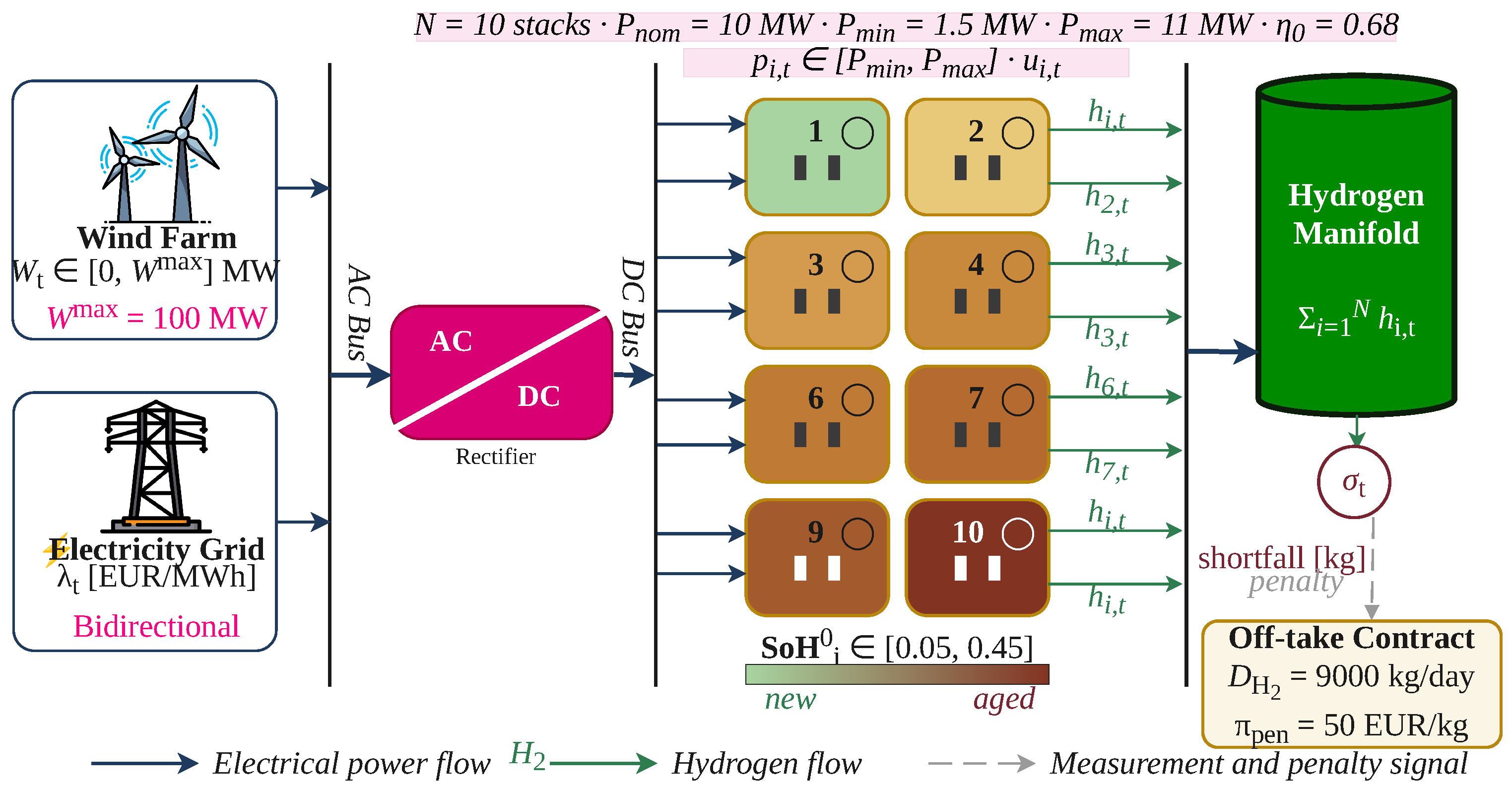
The plant of interest comprises N low-temperature electrolyser stacks operating in parallel and supplied jointly by a co-located wind farm and the day-ahead electricity market. Each stack has nominal power $P_{\mathrm{nom}}=10$ MW, so that the aggregate installed capacity reaches $N{P}_{\mathrm{nom}}=100$ MW for the reference configuration ($N=10$). The hydrogen produced is delivered to a downstream off-taker under a firm daily contract, and any undelivered volume is monetised through a shortfall penalty ${\pi }_{\mathrm{pen}}$ that captures both the contractual clauses and the reputational loss associated with supply disruption. Figure 1 depicts the resulting system architecture, which organises the $N=10$ stacks on a shared DC bus fed by a common rectifier interface from the upstream AC bus, and delivers the aggregate hydrogen output through a manifold to the firm daily off-take contract subject to the shortfall-penalty mechanism.

The scheduling horizon spans one operating day discretised in $T=24$ hourly intervals indexed by $t\in \mathcal{T}=\{1,\dots ,T\}$. Stacks are indexed by $i\in \mathcal{I}=\{1,\dots ,N\}$, and uncertainty realisations (scenarios) by $s\in \mathcal{S}=\{1,\dots ,S\}$ with associated probabilities ${\pi }_s$ that satisfy ${\sum }_{s\in \mathcal{S}}{\pi }_s=1$.

The choice of a heterogeneous fleet with $N>1$ is deliberate. Modern PtX plants operate stacks of mixed vintage because capacity is installed in tranches across several years, and therefore the initial state of health (SoH) is rarely uniform across the fleet. Accordingly, we model a linear initial SoH spread ${\mathrm{SoH}}_i^0=0.05+(i-1)\Delta \mathrm{SoH}$ with $\Delta \mathrm{SoH}=0.044$, which ranges from $5\%$ to $45\%$ of cumulated wear and is directly visible through the colour coding of the ten stack icons in Figure 1. This choice allows us to investigate whether the optimiser actively exploits the degradation heterogeneity when allocating duty cycles, which is an aspect that the deterministic baselines defined in Section 5.3 are unable to capture.

2.2. Electrolyser Dispatch and Commitment Model

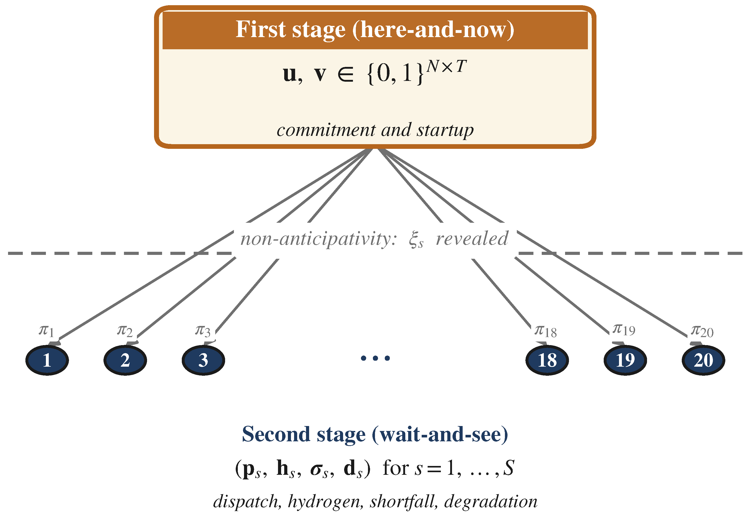
The decision variables are partitioned according to the two-stage stochastic programming paradigm [50]. First-stage here-and-now decisions are taken before the uncertainty is revealed and model the unit commitment of each stack. Specifically, $u_{i,t}\in \{0,1\}$ denotes whether stack i is committed at hour t, and $v_{i,t}\in \{0,1\}$ marks the startup event that occurs whenever stack i transitions from off to on. Second-stage wait-and-see decisions depend on the scenario index s and encompass the power dispatch $p_{i,t,s}\in {\mathbb{R}}_{\ge 0}$, the hydrogen output $h_{i,t,s}\in {\mathbb{R}}_{\ge 0}$, the monetised degradation cost $d_{i,s}\in {\mathbb{R}}_{\ge 0}$, and the hourly shortfall ${\sigma }_{t,s}\in {\mathbb{R}}_{\ge 0}$.

The electrolyser load of each committed stack must remain between its technical minimum and maximum:

$$\begin{array}{cccc}\hfill p_{i,t,s}& \le P_{\max }{u}_{i,t},\hfill & \hfill & \forall i,t,s,\hfill \\ \hfill p_{i,t,s}& \ge P_{\min }{u}_{i,t},\hfill & \hfill & \forall i,t,s,\hfill \end{array}$$

(1)

where $P_{\max }=1.10P_{\mathrm{nom}}=11$ MW accommodates a moderate overload that is standard in current PEM technology, and $P_{\min }=0.15P_{\mathrm{nom}}=1.5$ MW represents the minimum safe load below which water management and gas crossover become problematic [51,52]. Dispatch is also constrained by the realised wind power $W_{t,s}$:

$$\sum _{i\in \mathcal{I}}{p}_{i,t,s}\le W_{t,s},\forall t,s,$$

(2)

which implicitly rules out imported electricity outside the renewable envelope and therefore forces the plant to operate in a fully green-certified regime. This design choice is motivated by the European Delegated Act on Renewable Fuels of Non-Biological Origin (RFNBO), which mandates temporal and geographical correlation between renewable generation and electrolyser consumption for the produced hydrogen to qualify as “green” under the EU taxonomy. Although a bounded grid-import variable with a carbon-intensity penalty and a grid-export revenue term would extend the formulation to hybrid green/grey regimes and enable arbitrage during negative-price events, Equation (2) preserves the regulatory traceability required by the current certification framework. The relaxation of this constraint is identified as a future research direction in Section 7. The startup indicator follows the usual lower bound on the state transition:

$$v_{i,t}\ge u_{i,t}-u_{i,t-1},\forall i,\forall t\ge 2,$$

(3)

with $v_{i,t}\ge 0$. An aggregate plant-level ramping capability is introduced through

$$\left|\sum _{i\in \mathcal{I}}{p}_{i,t,s}-\sum _{i\in \mathcal{I}}{p}_{i,t-1,s}\right|\le R_{max},\forall t\ge 2,\forall s,$$

(4)

with $R_{max}=6$ MW/h reflecting the balance-of-plant constraint of the wind farm interconnection. The startup cost ${\pi }_{\mathrm{start}}=EUR800$ per event represents a complete cold-start cost that includes the energy consumed during the pre-heating ramp, the nitrogen purge of the gas channels, the deionised-water conditioning, and the auxiliary power for the balance-of-plant subsystems. This figure is consistent with the cold-start costs documented in the recent literature for MW-scale PEM electrolysers [52,53]. In industrial practice, warm starts (i.e., restarts within a short idle window during which the stack temperature remains above the minimum operating threshold) incur substantially lower costs, typically 30 to 50% of the cold-start figure. However, distinguishing between hot and cold starts in the MILP formulation would require additional binary variables encoding the time elapsed since the last shutdown together with minimum-downtime constraints. Since this extension would increase the number of integer variables from 480 to approximately 720 and would obscure the central contribution of the paper, the conservative cold-start assumption is adopted as an upper bound on the startup-related cost throughout this study.

The hourly hydrogen output of each stack follows the approximately linear Faraday relationship that is standard in techno-economic assessments of large-scale electrolysers [51,52]:

$$h_{i,t,s}={\displaystyle \frac{{\eta }_0{10}^3}{{\mathrm{LHV}}_{{\mathrm{H}}_2}}}{p}_{i,t,s},$$

(5)

where ${\eta }_0=0.68$ is the reference HHV-based efficiency, ${\mathrm{LHV}}_{{\mathrm{H}}_2}=33.33$ kWh/kg, and the factor ${10}^3$ converts power from MW to kW. The resulting conversion coefficient is approximately $20.4$ kg per MWh of electrical input, which is consistent with state-of-the-art PEM performance reported in the literature. Although ${\eta }_0$ is in practice mildly load-dependent, assuming it constant over the narrow range $[P_{\min },P_{\max }]$ introduces a negligible error and preserves the linearity required by the mixed-integer programming formulation.

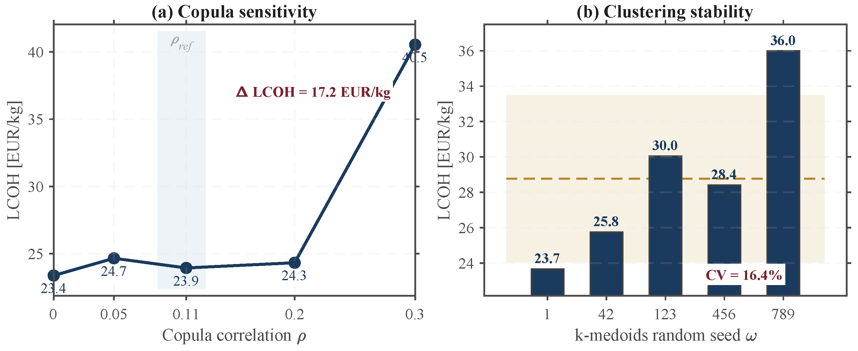
The constant efficiency assumption ${\eta }_0=0.68$ adopted in Equation (5) is a standard simplification in techno-economic MILP formulations for large-scale electrolysers [51]. In practice, the efficiency curve varies by approximately $\pm 3$–$5\%$ over the $[0.15,1.10]$ normalised load range. Introducing a load-dependent efficiency would render the hydrogen output $h_{i,t,s}$ a non-linear function of $p_{i,t,s}$, thereby breaking the linearity of the Faraday equality (5) and requiring a second piecewise linear approximation of the efficiency curve. Since the degradation model already introduces a PWL structure with $K=8$ breakpoints, adding a second PWL layer for efficiency would substantially increase the constraint count without a commensurate improvement in scheduling quality. The expected impact on LCOH ($\pm 3$–$5\%$) is small relative to the $14\%$ variation observed in the copula sensitivity analysis of Table 10.

2.3. Piecewise Linear Degradation Accounting

Degradation is by far the least standardised element in existing PtX scheduling models, since it couples non-convex electrochemical ageing phenomena with operational decisions. Empirical studies [54,55] show that voltage drift exhibits a distinctive U-shaped dependence on operating load, with a heavy penalty at low load (attributed to shunt currents and bubble coverage), a plateau in the mid-range where wear is minimal, and a steep rise above nominal load (attributed to mechanical stress and membrane thinning). In addition, every start–stop cycle inflicts a discrete damage increment linked to thermal-mechanical stresses at electrode interfaces [54]. To retain mixed-integer linear programming tractability while preserving these essential features, we approximate the instantaneous voltage drift rate by the upper envelope of K affine segments anchored at operating-regime breakpoints.

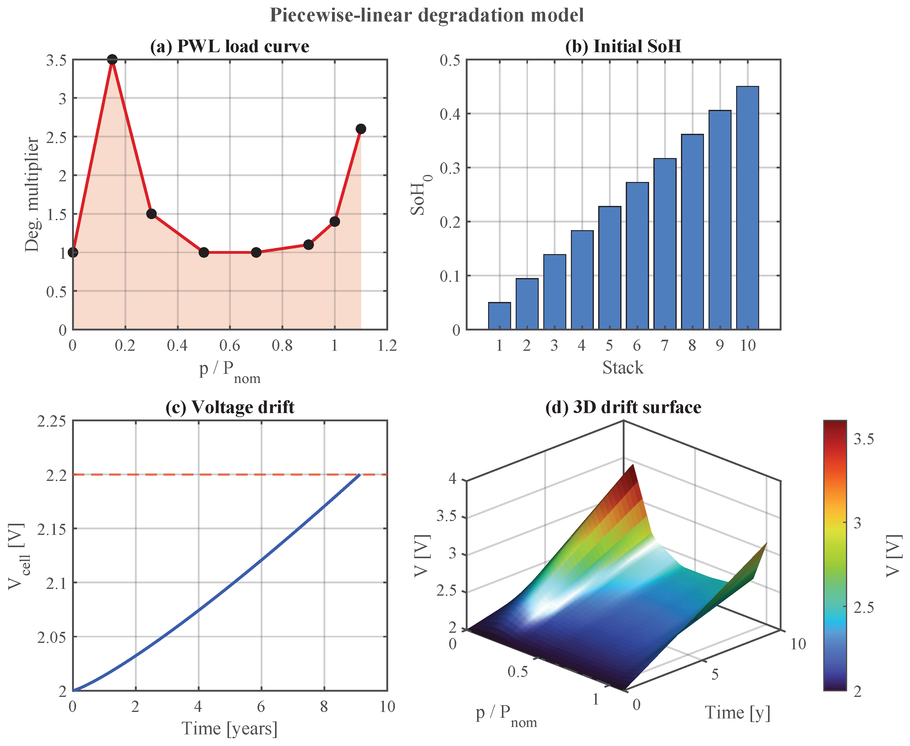
Let ${\tilde{p}}_{i,t,s}=p_{i,t,s}/P_{\mathrm{nom}}$ denote the dimensionless load. The breakpoints $\mathcal{B}$ and the associated degradation multipliers $\mathbf{\mu }$ are set to

$$\begin{array}{cc}\hfill \mathcal{B}& =\left\{0.00,0.15,0.30,0.50,0.70,0.90,1.00,1.10\right\},\hfill \\ \hfill \mathbf{\mu }& =\left\{1.0,3.5,1.5,1.0,1.0,1.1,1.4,2.6\right\},\hfill \end{array}$$

(6)

as illustrated in Figure 13a.  The multipliers have been calibrated so that the mid-range window $[0.5,0.9]$ of nominal load is the least damaging regime, in line with the stress-rupture curves reported in [54].

Specifically, the breakpoints and multipliers are calibrated against the experimental stress-rupture data of Frensch et al. [54] and Weiß et al. [55], which document the U-shaped voltage-drift dependence on operating load for PEM electrolysers: $\mathrm{\mu }=3.5$ at $\tilde{p}=0.15$ reflects experimentally observed shunt currents and bubble coverage at low load, $\mathrm{\mu }\approx 1.0$ in $[0.5,0.9]$ corresponds to the minimum-wear operating window, and $\mathrm{\mu }=2.6$ at $\tilde{p}=1.10$ captures overload-induced mechanical stress and membrane thinning.

Degradation is translated into a monetary equivalent by scaling the voltage drift through the capital-recovery coefficient

$$\kappa ={\displaystyle \frac{C_{\mathrm{CAPEX}}^{\mathrm{stack}}}{V_{\mathrm{eol}}-V_{\mathrm{nom}}}},$$

(7)

with $C_{\mathrm{CAPEX}}^{\mathrm{stack}}=EUR8$ M  $V_{\mathrm{nom}}=2.00$ V and $V_{\mathrm{eol}}=2.20$ V, which yields $\kappa =EUR4·{10}^7$/V. This quantity represents the monetised cost of one volt of permanent cell drift and is consistent with the end-of-life definition adopted in [52,53].

The per-stack degradation cost is represented through the epigraph variable $d_{i,s}$ constrained by the K linear cuts

$$\begin{array}{cc}\hfill d_{i,s}\ge \kappa \Delta t& [d_{\mathrm{load}}^{\mathrm{ref}}{\mathrm{\mu }}_k\sum _{t\in \mathcal{T}}{\tilde{p}}_{i,t,s}\hfill \\ \hfill & +d_{\mathrm{cycle}}^{\mathrm{ref}}\sum _{t\in \mathcal{T}}{v}_{i,t}],k=1,\dots ,K,\forall i\in \mathcal{I},\forall s\in \mathcal{S}.\hfill \end{array}$$

(8)

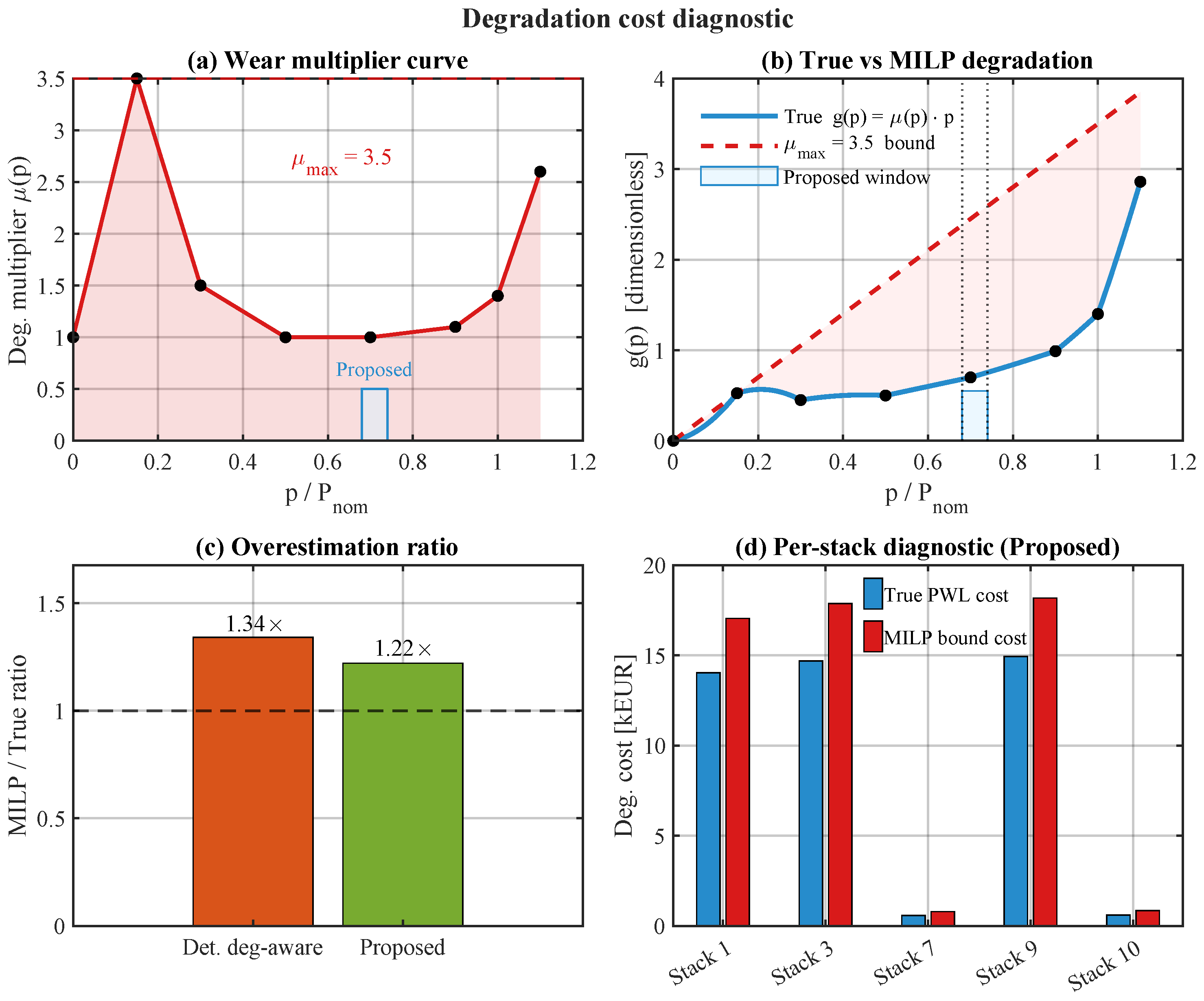
where $d_{\mathrm{load}}^{\mathrm{ref}}=6·{10}^{-6}$ V/h is the baseline load-induced drift rate and $d_{\mathrm{cycle}}^{\mathrm{ref}}=1.5·{10}^{-4}$ V per start–stop is the cycling damage increment. Because the objective minimises $d_{i,s}$, the tightest cut among the K constraints becomes automatically active. In the present formulation, all K lines pass through the origin with slope ${\mathrm{\mu }}_k·d_{\mathrm{load}}^{\mathrm{ref}}·\kappa /P_{\mathrm{nom}}$, which means the constraint corresponding to ${\mathrm{\mu }}_{max}=3.5$ is always the tightest for any positive aggregate dispatch ${\sum }_t{p}_{i,t,s}>0$. The epigraph therefore implements a conservative convex relaxation that assigns degradation at the worst-case multiplier regardless of the actual load level, providing a conservative upper bound on the true load-dependent cost. A dedicated diagnostic analysis (Figure 2) demonstrates that the overestimation ratio is $1.22\times$ for the proposed method and $1.34\times$ for the deterministic degradation-aware baseline, confirming that the conservatism is mild because the cycling term $d_{\mathrm{cycle}}^{\mathrm{ref}}\kappa {\sum }_t{v}_{i,t}$, which is identical in both the true and MILP calculations, constitutes a substantial fraction of the total degradation cost. Since all five benchmark methods employ the same formulation, the relative rankings, the ablation decomposition, and all comparative conclusions remain fully valid. The absolute LCOH values are mildly inflated by approximately 10–$15\%$, which represents the price of computational tractability within the linear programming framework. This construction avoids additional binary variables while preserving the monotone upper-envelope structure of $\mathrm{\mu }\left(\tilde{p}\right)$. Figure 13c,d illustrates the resulting voltage drift trajectory and its three-dimensional load-time projection, confirming that nominal operation at $\tilde{p}\simeq 1$ exhausts the voltage budget within the expected lifetime of $L_{\mathrm{stack}}$ = 80,000 h.

A terminological clarification is in order at this point. The elevated multiplier $\mathrm{\mu }\left(\tilde{p}\right)=3.5$ at $\tilde{p}=0.15$ that defines the low-load branch of the PWL envelope of Equations (6)–(8) captures the wear incurred when an active (committed) stack is operated below its plateau band, which is attributed in the experimental literature to shunt currents, bubble coverage at the electrode interface and the unstable water management characteristic of low-current operation [54,55]. This low-load damage is therefore a load-dependent mechanism that scales with the cumulative dispatch ${\sum }_t{\tilde{p}}_{i,t,s}$ of the committed stack and is fully captured by the load term of Equation (8).

Three distinct degradation mechanisms are captured by the formulation. First, load-dependent degradation is modelled through the PWL multiplier $\mathrm{\mu }\left(\tilde{p}\right)$ in Equation (8), which scales the cumulative dispatch of each committed stack and penalises both the under-load and over-load regimes. Second, start–stop cycling is captured by the separate term $d_{\mathrm{cycle}}^{\mathrm{ref}}\kappa {\sum }_t{v}_{i,t}$, which inflicts a discrete voltage damage increment of $1.5\times {10}^{-4}$ V per cycle independently of the load level. Third, idle degradation is parametrised by $d_{\mathrm{idle}}^{\mathrm{ref}}=2.5\times {10}^{-6}$ V/h in Table 5; idle stacks ($u_{i,t}=0$) contribute zero dispatch and therefore incur zero degradation cost through Equation (8). This idle drift rate enters only through the inter-day SoH update in the multi-day rolling-horizon extension discussed in Section 7.

An important scoping remark is necessary regarding the temporal treatment of the state of health. The present formulation computes the degradation cost over the single-day scheduling horizon of $T=24$ h without dynamically updating the SoH across consecutive days. Within a single day, the cumulative voltage drift is on the order of ${10}^{-4}$ V, which corresponds to less than $0.05\%$ of the total end-of-life voltage budget $(V_{\mathrm{eol}}-V_{\mathrm{nom}}=0.20$ V). This increment is well below the numerical resolution of the MILP solver and does not meaningfully alter the dispatch decisions. The present work therefore adopts a single-day approximation in which the initial SoH vector $\left\{{\mathrm{SoH}}_i^0\right\}$ is treated as a fixed parameter. A multi-day rolling-horizon extension with inter-day SoH coupling is identified as a priority research direction in Section 7.

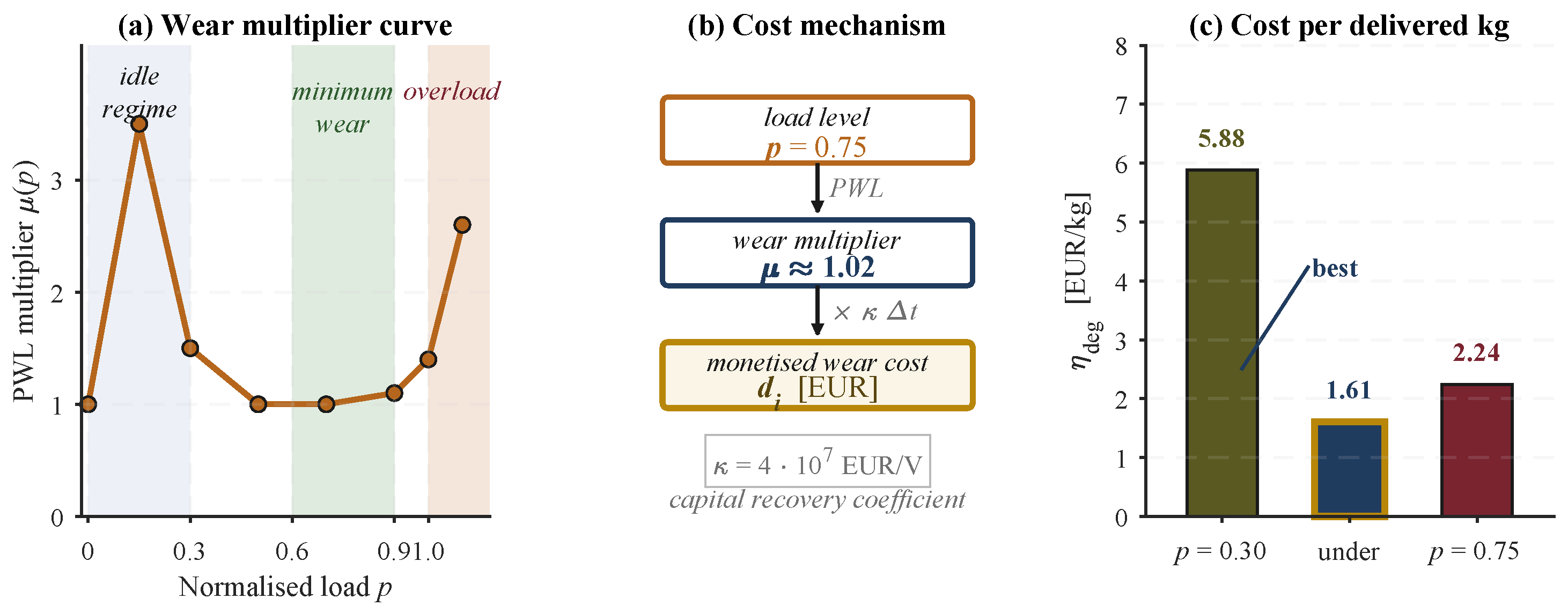
Figure 3 consolidates the graphical reading of the piecewise linear degradation model defined in Equations (6)–(8) into three complementary panels that together establish the central mechanical argument of the proposed framework. Panel (a) displays the daily-average wear multiplier $\mathrm{\mu }\left(\tilde{p}\right)$ across the full load range and makes the three operating regimes of the model visually explicit: an idle-damage regime for $\tilde{p}\in [0,0.30]$, in which the multiplier rises to $\mathrm{\mu }=3.5$ at $\tilde{p}=0.15$ under the combined effect of shunt currents and bubble coverage at the electrode interface; a minimum-wear plateau for $\tilde{p}\in [0.6,0.9]$, in which the multiplier stabilises at $\mathrm{\mu }\approx 1.0$ and the stack operates in the least damaging band; and an overload regime for $\tilde{p}>1$, in which the multiplier climbs again to $\mathrm{\mu }=2.6$ at $\tilde{p}=1.10$ under thermal stress and membrane thinning. The U-shape visible in panel (a) is therefore not an arbitrary calibration choice but a direct translation of the stress-rupture mechanisms documented in the experimental literature [54,55].

Panel (b) of Figure 3 traces the monetisation chain ${\tilde{p}}^{\circ }\to \mathrm{\mu }\left({\tilde{p}}^{\circ }\right)\to \kappa ·\mathrm{\mu }\left({\tilde{p}}^{\circ }\right)·\Delta t$ through which a single instantaneous load is converted into a monetised wear cost $d_i^{\circ }$, with the capital recovery coefficient $\kappa =EUR4·{10}^7$/V calibrated from the stack CAPEX and the voltage budget through Equation (7). This panel makes Equation (8) visually intuitive: a reader can trace the conversion from a load value to a monetised degradation cost in three steps, namely (i) reading the multiplier $\mathrm{\mu }\left({\tilde{p}}^{\circ }\right)$ from the PWL curve of panel (a), (ii) multiplying by the reference voltage drift rate $d_{\mathrm{load}}^{\mathrm{ref}}$ and the time step $\Delta t$, and (iii) multiplying by $\kappa$ to obtain the result in euros. Panel (c) reports the resulting marginal per-kilogram degradation cost ${\eta }_{\mathrm{deg}}\left(\tilde{p}\right)$ at three reference operating points: an under-loaded point at $\tilde{p}=0.30$, an in-plateau point at $\tilde{p}=0.75$, and an overloaded point at $\tilde{p}=1.05$. The three numerical values that populate the bars of panel (c) are reported in

Table 2. Marginal per-kilogram degradation cost at three reference operating points, computed from the PWL coefficients.

Operating Point	$\tilde{\mathit{p}}$	${\mathit{p}}_{\mathit{i}}$	$\mathsf{\mu }$	${\mathit{h}}_{\mathit{i}}$	${\mathit{\eta }}_{\mathbf{deg}}$
	[–]	[MW]	[–]	[kg/h]	[EUR/kg]
Under-loaded	0.30	3.0	1.50	61.21	5.88
In-plateau	0.75	7.5	1.03	153.02	1.62
Overloaded	1.05	10.5	2.00	214.22	2.24

Notes. The PWL multiplier $\mathrm{\mu }$ is computed by linear interpolation on the breakpoints $\mathit{\beta }=[0,0.15,0.30,0.50,0.70,0.90,1.00,1.10]$ and the multipliers $\mathbf{\mu }=[1.0,3.5,1.5,1.0,1.0,1.1,1.4,2.6]$. The hourly hydrogen production is $h_i={\eta }_0{p}_i·{10}^3/{\mathrm{LHV}}_{H_2}$ with ${\eta }_0=0.68$ and ${\mathrm{LHV}}_{H_2}=33.33$ kWh/kg. The hourly wear cost is ${\dot{d}}_i=\kappa ·d_{\mathrm{load}}^{\mathrm{ref}}·\mathrm{\mu }\left({\tilde{p}}_i\right)·\Delta t$, with $\kappa =EUR4.00·{10}^7/$V and $d_{\mathrm{load}}^{\mathrm{ref}}=6·{10}^{-6}$ V per 1000 h. The plateau value ${\eta }_{\mathrm{deg}}=EUR$ 1.62/kg is highlighted in bold.

, which is introduced in the following paragraph.

The numerical values used to construct panel (c) of Figure 3 are consolidated in Table 2. Each row reports, for a given normalised load $\tilde{p}$, the corresponding stack power $p_i$, the PWL multiplier $\mathrm{\mu }$ obtained by linear interpolation on the breakpoints $\mathit{\beta }$, the hourly hydrogen production $h_i$ computed from the nominal efficiency ${\eta }_0$ and the lower heating value ${\mathrm{LHV}}_{{\mathrm{H}}_2}$, the hourly degradation cost ${\dot{d}}_i$ derived from the capital recovery coefficient $\kappa$ and the reference voltage drift rate $d_{\mathrm{load}}^{\mathrm{ref}}=6·{10}^{-6}$ V/h, and the marginal per-kilogram degradation cost ${\eta }_{\mathrm{deg}}={\dot{d}}_i/h_i$. All five quantities are computed directly from the plant parameters declared in Section 5.1 and Table 5, so that every number displayed in the table and in panel (c) of Figure 3 is fully traceable to the declared inputs of the case study. The in-plateau point at $\tilde{p}=0.75$ reaches the minimum marginal cost of EUR $1.61$/kg, the under-loaded point at $\tilde{p}=0.30$ climbs to EUR $5.88$/kg, and the overloaded point at $\tilde{p}=1.05$ sits at EUR $2.24$/kg.

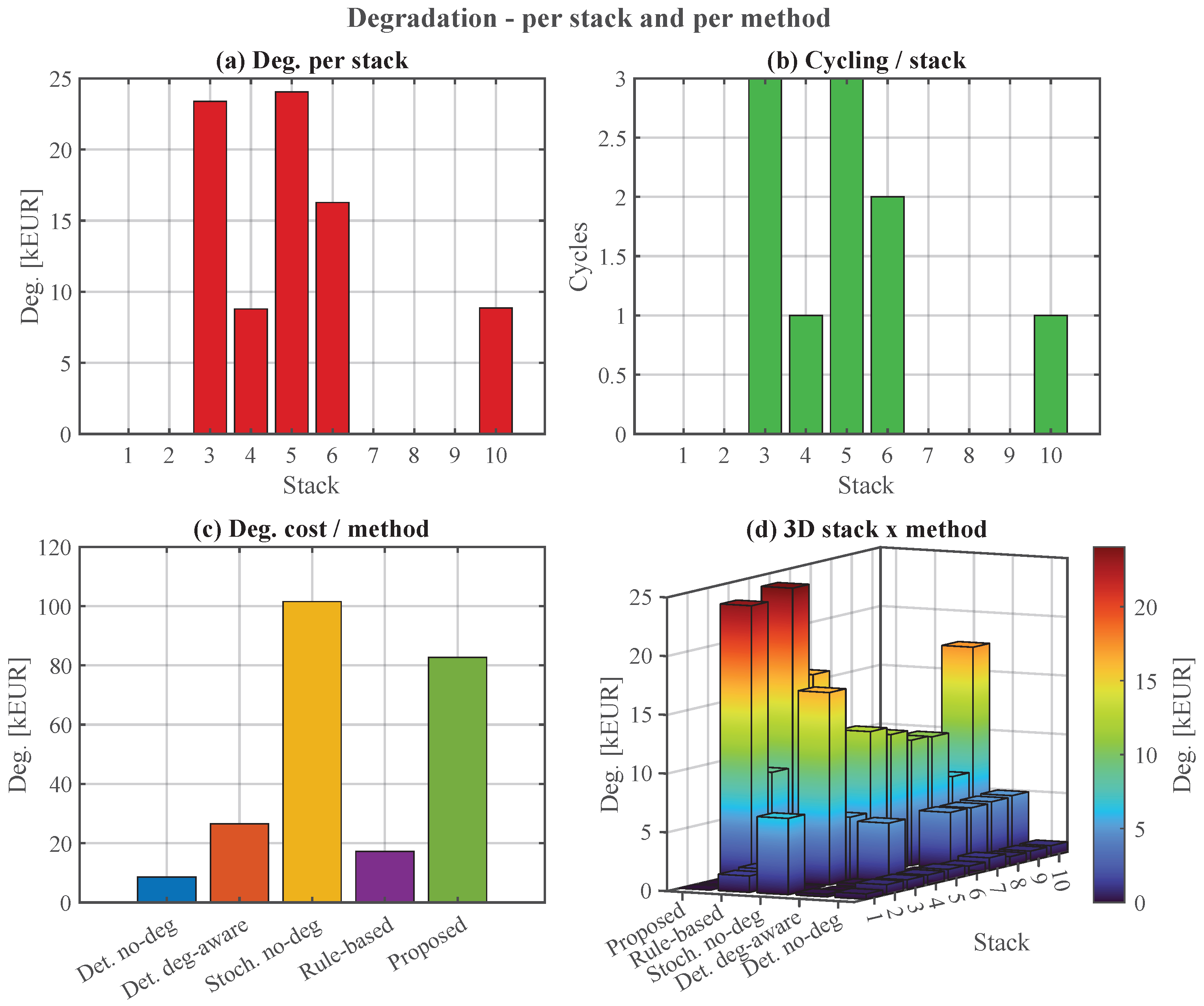
Expressed in monetary terms, the true PWL curve implies that keeping a committed stack in the mid-load band saves approximately EUR $4.27$ for every kilogram of hydrogen produced relative to the under-load regime and approximately EUR $0.63$ per kilogram relative to the over-load regime. Because the implemented MILP uses the conservative upper-bound degradation proxy described above, these savings are not directly captured by the solver; however, the conservative bound penalises high cumulative dispatch, which indirectly favours moderate per-stack loading. The ex-post diagnostic of Figure 2 confirms that the resulting dispatch falls within the mid-load band $\tilde{p}\in [0.68,0.74]$, where the true wear multiplier is near its minimum.

2.4. Joint Wind Price Uncertainty and Scenario Generation

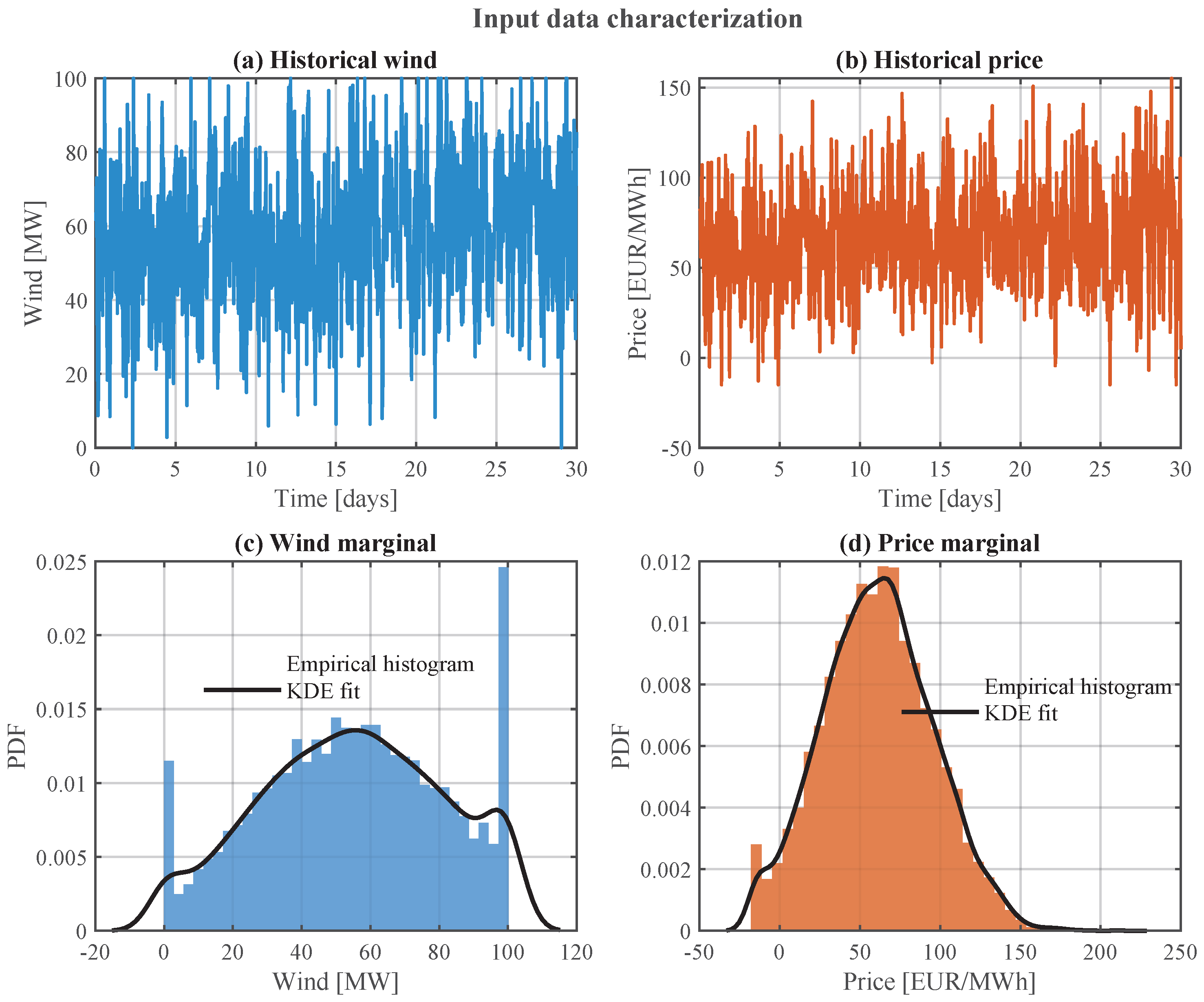
Wind generation and day-ahead electricity prices are modelled as the bivariate random process $(W_t,{\lambda }_t)$ whose joint distribution must be calibrated from a synthetic calibration sample. Figure 7a,b displays a representative monthly window of the hourly series used in this work. Both marginals exhibit non-Gaussian tails, and their coupling is asymmetric: large wind events tend to depress market prices because of merit-order effects, whereas low wind events produce price spikes driven by the residual demand that must be covered by thermal generation. A bivariate normal assumption is therefore inappropriate, as it would impose symmetric Gaussian tails and would not preserve the empirical marginals. Following established practice in energy applications [56,57], we adopt the Gaussian copula model combined with empirical marginals, which decouples the marginal calibration from the dependence structure and supports arbitrary tail shapes.

Let $F_W$ and $F_{\lambda }$ denote the empirical cumulative distribution functions estimated from the synthetic calibration series via the empirical CDF. Each observation is transformed into the uniform domain through $u_t^W=F_W\left(W_t\right)$ and $u_t^{\lambda }=F_{\lambda }\left({\lambda }_t\right)$, and subsequently mapped into the standard Gaussian domain via the probit transform $z={\Phi }^{-1}\left(u\right)$. The rank correlation of the transformed pairs,

$$\widehat{\rho }=\mathrm{corr}\left({\Phi }^{-1}\left(F_W\left(W\right)\right),{\Phi }^{-1}\left(F_{\lambda }\left(\lambda \right)\right)\right),$$

(9)

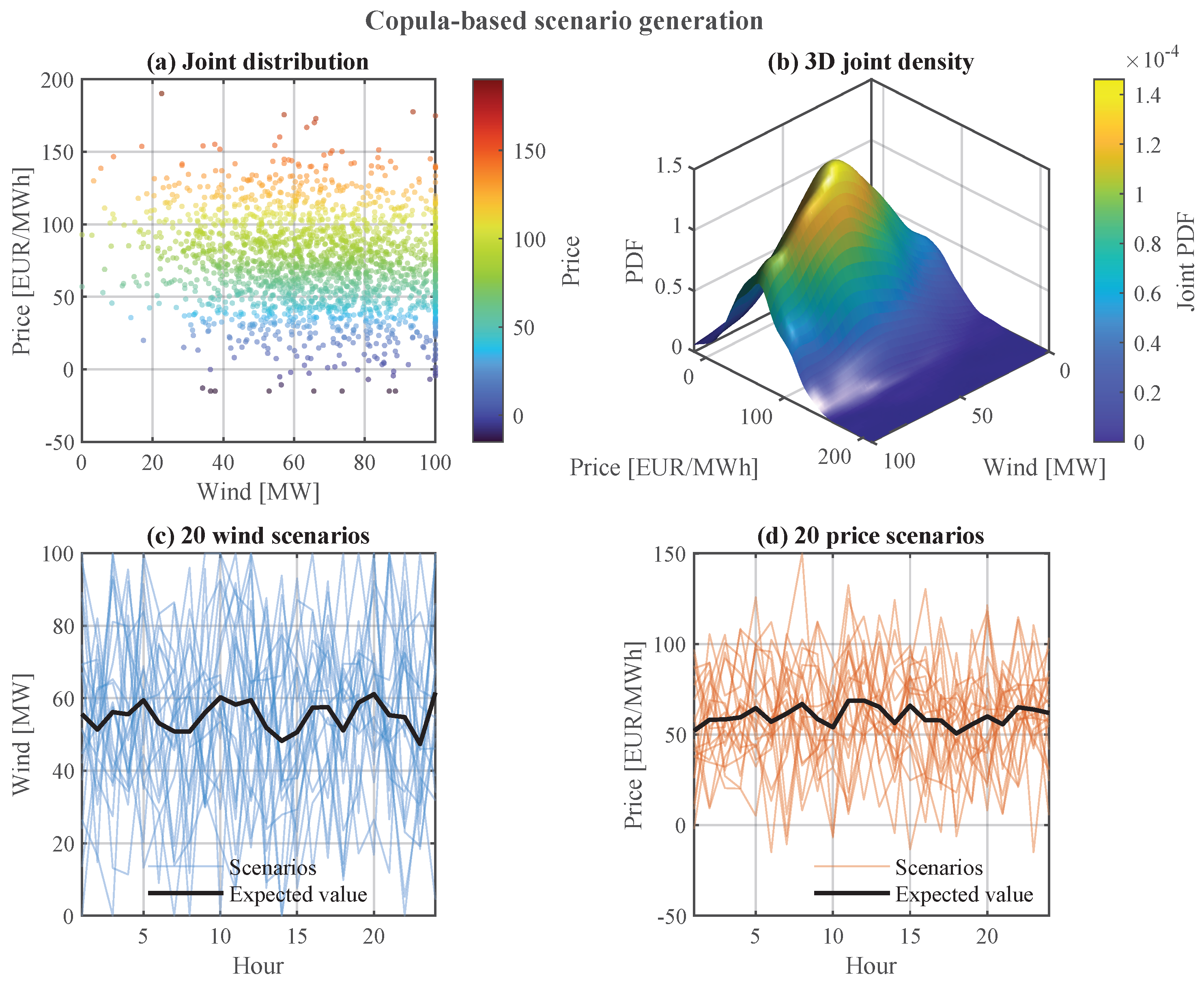
is the single parameter of the Gaussian copula. For the dataset considered in this study, $\widehat{\rho }\simeq 0.11$, indicating a weak but non-negligible coupling. Figure 8a shows the empirical scatter used in the fit, and Figure 8b reports the resulting bivariate kernel density estimate, which reproduces the single-mode structure near $(55\mathrm{MW},80\mathrm{EUR}/\mathrm{MWh})$ together with the asymmetric price tail.

Synthetic scenarios are generated in three steps. First, a pool of M normal samples is drawn from $\mathcal{N}(\mathbf{0},\Sigma )$ with

$$\Sigma =\left(\begin{array}{cc}1& \widehat{\rho }\\ \widehat{\rho }& 1\end{array}\right).$$

(10)

Second, each sample is pushed through the standard normal CDF $\Phi$ to obtain uniform realisations, which are then mapped into the physical domain via the inverse empirical marginals $F_W^{-1}$ and $F_{\lambda }^{-1}$. Third, the pool is reduced to a tractable set of S representative trajectories via the k-medoids clustering algorithm [58], with squared Euclidean distance applied to the concatenated feature vector $[W_{1,m},\dots ,W_{T,m},{\lambda }_{1,m},\dots ,{\lambda }_{T,m}]$. The probability mass of each reduced scenario is set equal to the cluster cardinality divided by M, hence    

$${\pi }_s={\displaystyle \frac{|{\mathcal{C}}_s|}{M}},\sum _{s\in \mathcal{S}}{\pi }_s=1,$$

(11)

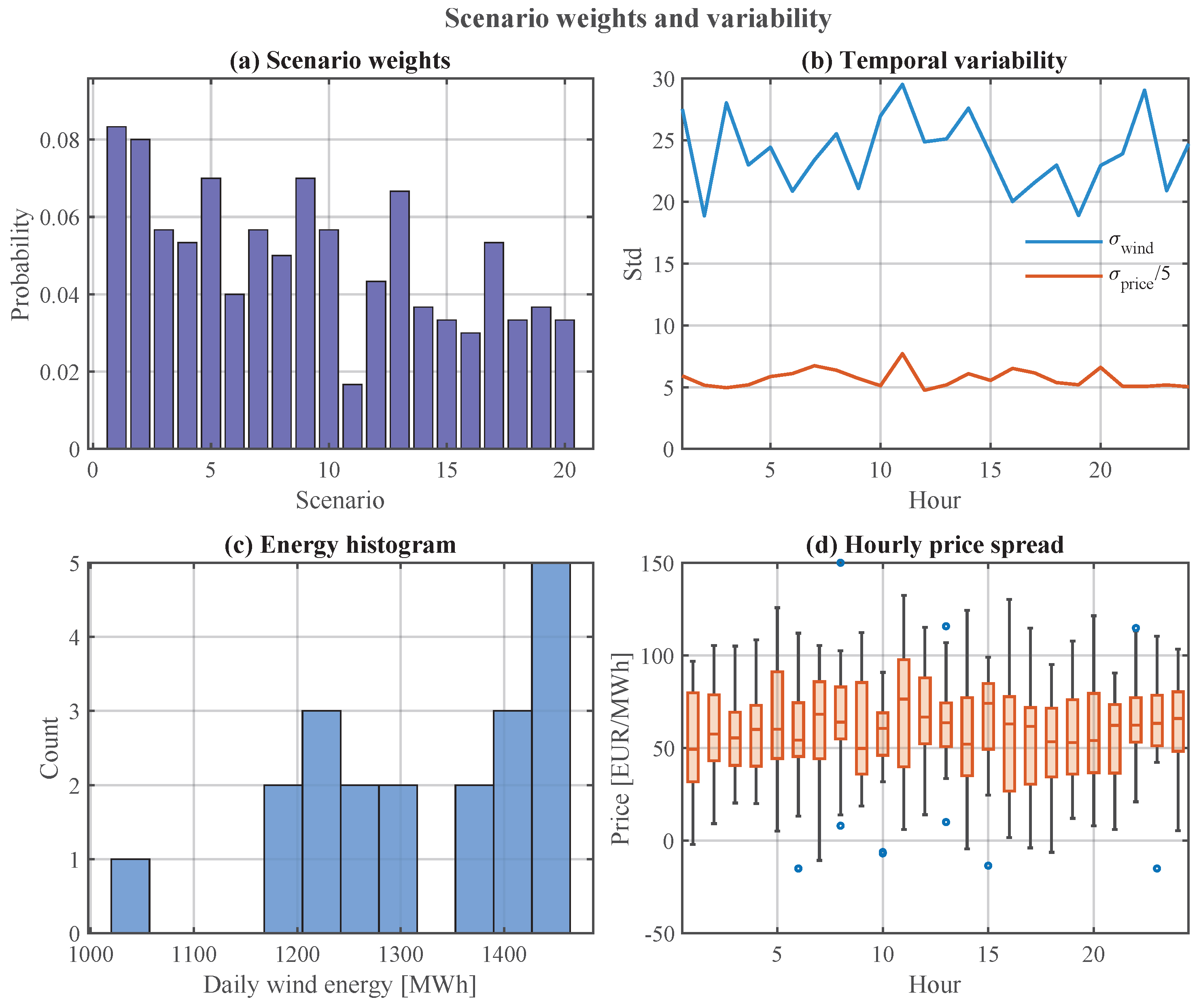
where ${\mathcal{C}}_s$ denotes the set of pool samples assigned to cluster s. In the reference configuration used throughout this paper, we set $M=300$ and $S=20$ for training. Figure 8c,d display the $S=20$ reduced wind and price trajectories together with their expected value, and Figure 9a reports the resulting scenario weights, which vary mildly around the uniform value $1/S=0.05$.

To prevent in-sample overfitting from inflating the reported savings, we enforce a strict out-of-sample protocol. A second independent sample of $M^{\prime }=500$ scenarios is generated with a different random seed and reduced to $S^{\prime }=50$ test trajectories. First-stage commitment decisions $(u_{i,t}^{★},v_{i,t}^{★})$ are computed on the training set and held fixed, after which the second-stage variables are re-optimised as a pure linear program, since no binary variable remains free, on each of the $S^{\prime }$ test realisations. This sample-splitting procedure is standard in stochastic programming [59], and it guarantees that the key performance indicators reported in Section 6 reflect genuine generalisation rather than in-sample optimism.

2.5. Economic Objective and Reliability Metric

The first-stage cost collects the cold-start charges, since commitment and startup decisions are taken before the uncertainty is revealed:

$$Z^{\left(1\right)}={\pi }_{\mathrm{start}}\sum _{i\in \mathcal{I}}\sum _{t\in \mathcal{T}}{v}_{i,t},$$

(12)

with ${\pi }_{\mathrm{start}}=EUR800$ per cold start, a figure consistent with the auxiliary-heating and pre-conditioning costs documented in [52]. The second-stage cost is the scenario-weighted sum of the forgone electricity revenue (opportunity cost), the monetised degradation, and the shortfall penalty:

$$\begin{array}{cc}\hfill Z^{\left(2\right)}=\sum _{s\in \mathcal{S}}{\pi }_s[& \sum _{t\in \mathcal{T}}{\lambda }_{t,s}\sum _{i\in \mathcal{I}}{p}_{i,t,s}+\sum _{i\in \mathcal{I}}{d}_{i,s}\hfill \\ \hfill & +{\pi }_{\mathrm{pen}}\sum _{t\in \mathcal{T}}{\sigma }_{t,s}-{\pi }_{{\mathrm{H}}_2}\sum _{i\in \mathcal{I}}\sum _{t\in \mathcal{T}}{h}_{i,t,s}],\hfill \end{array}$$

(13)

where the four scenario-weighted contributions correspond, in order, to the forgone electricity revenue (opportunity cost of consumed wind power) at the realised price ${\lambda }_{t,s}$, the monetised stack-level degradation cost $d_{i,s}$ defined through the piecewise linear epigraph of Equation (8), the shortfall penalty ${\pi }_{\mathrm{pen}}{\sum }_t{\sigma }_{t,s}$ that penalises any unmet portion of the daily contract, and the producer-side revenue ${\pi }_{{\mathrm{H}}_2}{\sum }_{i,t}{h}_{i,t,s}$ collected from the delivered hydrogen at the merchant price ${\pi }_{{\mathrm{H}}_2}$. The electricity price ${\lambda }_{t,s}$ in Equation (13) represents the opportunity cost of not selling the consumed wind power on the day-ahead market: every MWh of wind power directed to the electrolysers under Constraint (2) could alternatively have been sold at the prevailing market price ${\lambda }_{t,s}$, and the price term therefore captures the forgone electricity revenue. No grid electricity is purchased under the present formulation. The slack variable ${\sigma }_{t,s}\ge 0$ represents the hourly hydrogen shortfall and closes the daily demand balance

$$\sum _{i\in \mathcal{I}}\sum _{t\in \mathcal{T}}{h}_{i,t,s}+\sum _{t\in \mathcal{T}}{\sigma }_{t,s}\ge D_{{\mathrm{H}}_2},\forall s,$$

(14)

with $D_{{\mathrm{H}}_2}=9000$ kg per day, ${\pi }_{\mathrm{pen}}=EUR$ 50/kg and ${\pi }_{{\mathrm{H}}_2}=EUR$ 5.5/kg. The shortfall penalty is deliberately set above the prevailing hydrogen merchant price by roughly an order of magnitude so that physical feasibility is strictly preferred to monetary substitution, which is the standard convention in the robust supply-contract literature [59]. The merchant price ${\pi }_{{\mathrm{H}}_2}=EUR$ 5.5/kg corresponds to the lower end of the European green-hydrogen merchant range reported in recent techno-economic assessments [7] and is included in $Z^{\left(2\right)}$ to ensure that the scheduler perceives the opportunity cost of curtailed production at every dispatch decision. The complete expected total-cost objective of the stochastic MILP problem is then

$$\mathcal{J}=Z^{\left(1\right)}+Z^{\left(2\right)},$$

(15)

which the solver minimises jointly over the first- and second-stage variables subject to the constraints introduced in (1)–(14). For the comparative analysis of Section 6, we report the conventional cost-only metric

$${\mathcal{J}}_{\mathrm{cost}}^{★}=Z^{\left(1\right)}+Z^{\left(2\right)}+{\pi }_{{\mathrm{H}}_2}\sum _{s\in \mathcal{S}}{\pi }_s\sum _{i\in \mathcal{I}}\sum _{t\in \mathcal{T}}{h}_{i,t,s}^{★},$$

(16)

which nets the merchant revenue from the displayed expected total cost in order to remain compatible with the techno-economic conventions adopted in the recent multi-stack PtX literature [7]. This convention does not affect the optimal solution: the Faraday equality (5) renders hydrogen output a deterministic linear function of dispatch, so the revenue term adds a uniform per-MWh offset ${\pi }_{{\mathrm{H}}_2}·{\eta }_0·{10}^3/{\mathrm{LHV}}_{{\mathrm{H}}_2}$ to every dispatch cost coefficient $c_{p_{i,t,s}}$, identical across all stacks, scenarios, and time periods. Because this offset is constant and does not depend on any decision variable, it shifts the objective value by a fixed amount proportional to total dispatch without altering the argmin. The displayed cost-only metric ${\mathcal{J}}_{\mathrm{cost}}^{★}$ of Equation (16) simply reverses this offset for reporting purposes. It makes the headline LCOH and total-cost values directly comparable with the prior art.

To support the benchmark analysis of Section 6, we further report two key performance indicators. The first is the levelised cost of hydrogen, defined as

$$\mathrm{LCOH}={\displaystyle \frac{\mathcal{J}}{{\displaystyle {\mathbb{E}}_s\left[\sum _{i\in \mathcal{I}}\sum _{t\in \mathcal{T}}{h}_{i,t,s}\right]}}},$$

(17)

which expresses the delivered hydrogen cost in EUR/kg and encompasses all operational, degradation, and penalty terms. The second is the demand reliability

$$\mathrm{Rel}=1-{\displaystyle \frac{{\displaystyle {\mathbb{E}}_s\left[\sum _{t\in \mathcal{T}}{\sigma }_{t,s}\right]}}{D_{{\mathrm{H}}_2}}},$$

(18)

which quantifies the expected fraction of the daily contract that the plant honours. A value $\mathrm{Rel}=1$ indicates that the expected shortfall is zero across all test realisations, whereas $\mathrm{Rel}<1$ flags the probability-weighted under-delivery. Together, LCOH and Rel form a two-objective evaluation envelope: a low LCOH is meaningful only if coupled with a high reliability, since methods that under-commit the fleet may appear artificially cheap per kilogram while failing to honour the supply contract. Accordingly, the joint reporting of both metrics in the Results section is essential to a balanced comparison between the proposed framework and the deterministic baselines.

In addition, the effective levelised cost ${\mathrm{LCOH}}_{\mathrm{eff}}={\mathcal{J}}^{★}/D_{{\mathrm{H}}_2}$ normalises the total cost by the contractual demand rather than by the realised production. The numerator ${\mathcal{J}}^{★}$ embeds the shortfall penalty ${\pi }_{\mathrm{pen}}{\sum }_t{\sigma }_{t,s}$, so any under-delivery inflates ${\mathrm{LCOH}}_{\mathrm{eff}}$ in direct proportion. Low-reliability methods are therefore penalised rather than artificially favoured.

3. Two-Stage Stochastic MILP Formulation

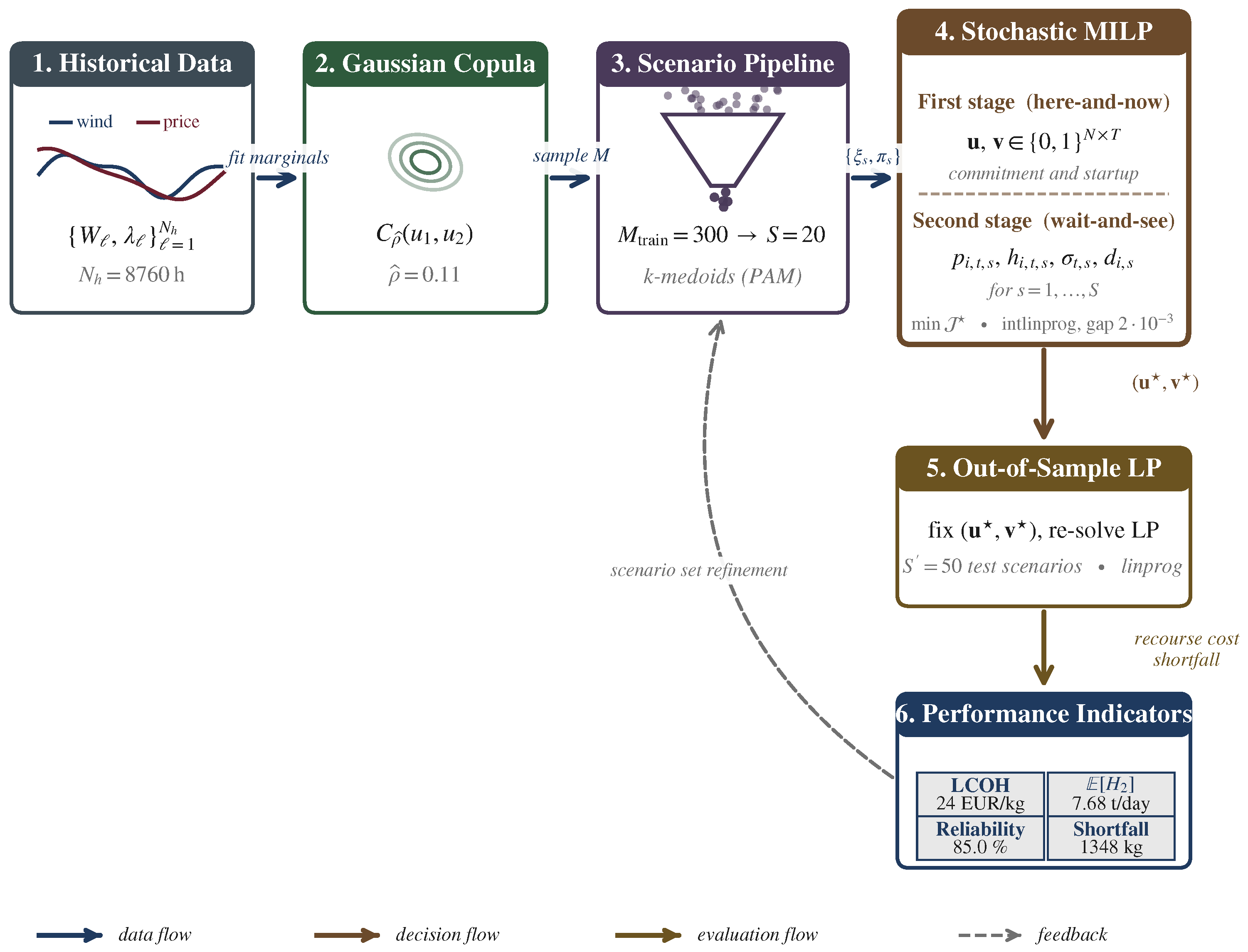
Section 2 introduced the physical plant model together with the individual constraint blocks and the cost structure. This section casts the whole problem as a single mixed-integer linear program in extensive form, which is the representation directly consumed by modern branch-and-cut solvers. Figure 4 summarises the full computational pipeline that the present section formalises, from the raw synthetic wind and price data through the copula-based scenario generation and the k-medoids reduction, to the two-stage MILP solver and the out-of-sample evaluation loop that produces the key performance indicators reported in Section 6. Section 3.1 recalls the abstract two-stage stochastic program and its deterministic equivalent under finite-scenario support. Section 3.2 assembles the stacked decision vector and the objective. Section 3.3 enumerates the constraint blocks and their dimensions. Section 3.4 discusses the sparse assembly, the solver deployment, and the effective levelised-cost metric used throughout the out-of-sample comparison.

3.1. Extensive-Form Stochastic Program

The abstract two-stage stochastic program reads

$$\underset{x\in \mathcal{X}}{min}{c}^{\top }x+{\mathbb{E}}_{\xi }\left[\mathcal{Q}(x,\xi )\right],$$

(19)

where x gathers the first-stage here-and-now decisions, $\xi$ is the random vector of exogenous data, and $\mathcal{Q}(x,\xi )$ is the optimal value of the second-stage recourse problem

$$\mathcal{Q}(x,\xi )=\underset{y\ge 0}{min}q{\left(\xi \right)}^{\top }y\mathrm{s}.\mathrm{t}.Wy\ge h\left(\xi \right)-Tx.$$

(20)

Under the finite-scenario support ${\left\{{\xi }_s\right\}}_{s\in \mathcal{S}}$ adopted in Section 2.4, the expectation in (19) collapses into a finite weighted sum. Introducing scenario-specific recourse variables $y_s$, the whole problem is rewritten in the extensive form    

$$\underset{x\in \mathcal{X},y_1,\dots ,y_S}{min}{c}^{\top }x+\sum _{s\in \mathcal{S}}{\pi }_s{q}_s^{\top }{y}_s,$$

(21)

subject to the first-stage constraints $Ax\le b$ and the scenario-specific recourse constraints $Tx+W{y}_s\le h_s$ for every $s\in \mathcal{S}$. Because x does not carry a scenario subscript, non-anticipativity is implicit and no additional equality constraint of the form $x_s=x_{s^{\prime }}$ is required. Equation (21) is the template against which the concrete Power-to-X problem is now aligned.

The two-stage decision structure formalised in this subsection is illustrated in Figure 5, which makes the non-anticipativity boundary between the first-stage commitment $(\mathbf{u},\mathbf{v})$ and the second-stage scenario-indexed recourse decisions $({\mathbf{p}}_s,{\mathbf{h}}_s,{\mathit{\sigma }}_s,{\mathbf{d}}_s)$ visually explicit.

3.2. Compact Vector Form

In the Power-to-X instance, the first-stage vector collects the commitment and startup indicators, that is $x=[\mathbf{u};\mathbf{v}]$ with $\mathbf{u},\mathbf{v}\in {\{0,1\}}^{NT}$. The second-stage vector gathers the dispatch, the hydrogen output, the shortfall, and the monetised degradation per scenario:

$$y_s=\left[{\mathbf{p}}_s;{\mathbf{h}}_s;{\mathit{\sigma }}_s;{\mathbf{d}}_s\right],{\mathbf{p}}_s,{\mathbf{h}}_s\in {\mathbb{R}}_{\ge 0}^{NT},{\mathit{\sigma }}_s\in {\mathbb{R}}_{\ge 0}^T,{\mathbf{d}}_s\in {\mathbb{R}}_{\ge 0}^N.$$

(22)

Stacking all second-stage variables across scenarios yields the global decision vector

$$z=\left[\mathbf{u};\mathbf{v};{\mathbf{p}}_1;\dots ;{\mathbf{p}}_S;{\mathbf{h}}_1;\dots ;{\mathbf{h}}_S;{\mathit{\sigma }}_1;\dots ;{\mathit{\sigma }}_S;{\mathbf{d}}_1;\dots ;{\mathbf{d}}_S\right]\in {\mathbb{R}}^{n_{\mathrm{var}}},$$

(23)

whose total dimension is

$$n_{\mathrm{var}}=\underset{\mathbf{u},\mathbf{v}}{\underbrace{2NT}}+\underset{\mathbf{p},\mathbf{h}}{\underbrace{2NTS}}+\underset{\mathit{\sigma }}{\underbrace{TS}}+\underset{\mathbf{d}}{\underbrace{NS}}.$$

(24)

For the reference configuration $(N,T,S)=(10,24,20)$ this gives $n_{\mathrm{var}}$ = 10,760 decision variables, of which $n_{\mathrm{int}}=2NT=480$ are binary and the remainder continuous.

The objective coefficients are assembled directly from Equations (12), (13), and (15) of Section 2. Specifically,    

$$\left\{\begin{array}{cccc}\hfill c_{v_{i,t}}& ={\pi }_{\mathrm{start}},\hfill & \hfill c_{u_{i,t}}& =0,\hfill \\ \hfill c_{p_{i,t,s}}& ={\pi }_s{\lambda }_{t,s},\hfill & \hfill c_{h_{i,t,s}}& =0,\hfill \\ \hfill c_{{\sigma }_{t,s}}& ={\pi }_s{\pi }_{\mathrm{pen}},\hfill & \hfill c_{d_{i,s}}& ={\pi }_s.\hfill \end{array}\right.$$

(25)

The hydrogen variables receive a zero coefficient in the displayed vector because the Faraday equality (5) eliminates $h_{i,t,s}$ as an independent variable: substituting $h_{i,t,s}=({\eta }_0·{10}^3/{\mathrm{LHV}}_{{\mathrm{H}}_2})p_{i,t,s}$ into the revenue term of Equation (13) yields an effective dispatch coefficient $c_{p_{i,t,s}}^{\mathrm{eff}}={\pi }_s{\lambda }_{t,s}-{\pi }_s{\pi }_{{\mathrm{H}}_2}{\eta }_0·{10}^3/{\mathrm{LHV}}_{{\mathrm{H}}_2}$, which absorbs the hydrogen revenue as a uniform negative offset on every dispatch variable. The zero on $c_{h_{i,t,s}}$ therefore reflects the elimination of h rather than the absence of the revenue term from the optimised objective. The resulting mixed-integer linear program in standard form reads

$$\begin{array}{|c|}\hline \begin{array}{cccc}\hfill & \underset{z}{min}\hfill & \hfill & c^{\top }z\hfill \\ \hfill & \mathrm{s}.\mathrm{t}.\hfill & \hfill & A_{\mathrm{ineq}}z\le b_{\mathrm{ineq}},\hfill \\ \hfill & \hfill & \hfill & A_{\mathrm{eq}}z=b_{\mathrm{eq}},\hfill \\ \hfill & \hfill & \hfill & lb\le z\le ub,\hfill \\ \hfill & \hfill & \hfill & z_j\in \{0,1\},j\in {\mathcal{J}}_{\mathrm{int}},\hfill \end{array}\\ \hline\end{array}$$

(26)

where ${\mathcal{J}}_{\mathrm{int}}$ is the index set of the binary entries and $(lb,ub)$ are the physical bounds assembled from Section 2.2.

3.3. Constraint Dimensioning

Table 3. Constraint blocks and row counts for the reference instance ($N=10$, $T=24$, $S=20$, $K=8$ piecewise linear breakpoints).

Constraint Family	Reference	Expression	Row Count
Power upper bound	(1)	$NTS$	4800
Power lower bound	(1)	$NTS$	4800
Wind availability	(2)	$TS$	480
Startup indicator	(3)	$N(T-1)$	230
Aggregate ramp $(\pm )$	(4)	$2(T-1)S$	920
PWL degradation cuts	(8)	$NSK$	1600
Demand balance	(14)	S	20
$A_{\mathrm{ineq}}$ total rows			12,850
H2 Faraday equality	(5)	$NTS$	4800
$A_{\mathrm{eq}}$ total rows			4800

enumerates the constraint families that populate $(A_{\mathrm{ineq}},A_{\mathrm{eq}})$, together with the corresponding equation in Section 2 and the resulting row count.

The inequality block therefore contains 12,850 rows and the equality block 4800 rows, giving a total of 17,650 constraints. Together with the 10,760 decision variables identified in Equation (24), a dense representation of the joint matrix would require over 190 million entries, the overwhelming majority of which are zero. The next subsection explains how the sparse triplet form avoids this storage overhead entirely.

3.4. Sparse Assembly, Solver Deployment, and Effective LCOH

Each constraint family in Table 3 contributes only a handful of non-zero entries per row. Specifically, the power-bound constraints touch two variables per row (the corresponding $p_{i,t,s}$ and $u_{i,t}$), the wind cap touches N, the ramp constraints touch $2N$, the PWL degradation cuts touch $T+1$, and the Faraday equality touches two. A conservative upper bound on the number of non-zeros is    

$$\mathrm{nnz}\left(A\right)\lesssim (11+K)NTS+\mathcal{O}\left(NT\right),$$

(27)

which for the reference instance evaluates to approximately $9.7·{10}^4$ entries, that is more than three orders of magnitude below the dense count. Accordingly, the constraint matrix is assembled through the coordinate triplet format $(\mathbf{i},\mathbf{j},\mathbf{v})$ and converted to compressed-sparse-column storage via the MATLAB intrinsic sparse(i,j,v,m,n). This construction preserves an $\mathcal{O}\left(\mathrm{nnz}\right)$ memory footprint and allows the MILP to be passed directly to intlinprog without any pre-conditioning step.

The solver is configured with a relative optimality gap of $2·{10}^{-3}$ and a maximum solution time of 180 s. For the reference instance, branch-and-bound explores only a few dozen nodes before certifying optimality within the prescribed gap, and the wall-clock time stays below 15 s on an Intel i7 desktop with 16 GB of RAM. When the plant size is doubled to $N=20$ stacks or the scenario count raised to $S=50$, the solution time grows approximately linearly in $n_{\mathrm{var}}$ thanks to the tight linear-programming relaxation induced by the epigraph piecewise linear formulation, which is markedly more efficient than the alternative $\mathcal{O}\left(\log K\right)$ binary encoding discussed in [60].

Out-of-sample evaluation follows the canonical sample-split protocol of stochastic programming [59]. The first-stage optimum $({\mathbf{u}}^{★},{\mathbf{v}}^{★})$ obtained from the training set is held fixed, after which the second-stage variables are re-optimised as a pure linear program, since no binary variable remains free, on each of the $S^{\prime }=50$ test scenarios independently. This LP re-dispatch uses MATLAB’s linprog with the dual-simplex algorithm and a vectorised sparse assembly that mirrors the training-time structure.

Two performance indicators are computed from the test-set solution. The first is the nominal levelised cost of hydrogen already introduced in Equation (17), which divides the expected cost by the expected hydrogen mass actually delivered. The second is the effective levelised cost

$${\mathrm{LCOH}}_{\mathrm{eff}}={\displaystyle \frac{{\mathcal{J}}^{★}}{D_{{\mathrm{H}}_2}}},$$

(28)

which fixes the denominator at the contractual demand rather than at the realised production. Because the numerator ${\mathcal{J}}^{★}$ embeds the shortfall penalty through Equation (13), any under-delivery inflates ${\mathrm{LCOH}}_{\mathrm{eff}}$ in direct proportion to the unmet volume. Reporting both LCOH and ${\mathrm{LCOH}}_{\mathrm{eff}}$ is essential to disentangle the apparent per-unit cost from the physical service level, as a method that commits too few stacks may display a low nominal LCOH while incurring a large ${\mathrm{LCOH}}_{\mathrm{eff}}$ driven by the penalty term. Accordingly, the benchmark analysis of Section 6 reports both metrics jointly so that the reliability dimension of each candidate policy remains visible.

4. Scenario Generation and Reduction

Section 3 treats the finite scenario set ${\left\{{\xi }_s\right\}}_{s\in \mathcal{S}}$ and its probability vector $\left\{{\pi }_s\right\}$ as a given input of the extensive-form MILP. This section details the statistical pipeline that produces this set from the raw synthetic calibration observations, covering four successive steps: empirical marginal calibration (Section 4.1), Gaussian copula fitting through rank transformation (Section 4.2), Monte Carlo sampling in the copula domain (Section 4.3), and cluster-based scenario reduction via k-medoids (Section 4.4). Section 4.5 closes the section with the out-of-sample partitioning protocol and the empirical validation of the reduced scenarios against the raw data moments illustrated in Figures 7–9.

4.1. Empirical Marginal Estimation

Let ${\left\{W_{\ell }\right\}}_{\ell =1}^{N_h}$ and ${\left\{{\lambda }_{\ell }\right\}}_{\ell =1}^{N_h}$ denote the hourly synthetic wind and electricity price series, with $N_h=8760$ observations covering one calendar year. The marginal cumulative distribution functions $F_W$ and $F_{\lambda }$ are estimated non-parametrically through the empirical CDF, which for a generic univariate sample $\left\{x_{\ell }\right\}$ of size $N_h$ yields

$${\widehat{F}}_X\left(x\right)={\displaystyle \frac{1}{N_h}}{\displaystyle \sum _{\ell =1}^{N_h}}\mathbf{1}\{x_{\ell }\le x\},$$

(29)

together with the step-wise inverse ${\widehat{F}}_X^{-1}\left(u\right)$ obtained by linear interpolation between the sorted order statistics. This construction is free of any parametric assumption about the tail shape, which is essential for wind generation and day-ahead price data because the classical Gaussian assumption is known to systematically underestimate the probability of extreme events [61]. Figure 7c,d display the wind and price histograms overlaid with their kernel density counterparts, and confirm the non-Gaussian character of both marginals: wind exhibits a bounded support with an accumulation near the upper limit, while price shows heavier right tails together with occasional negative excursions driven by oversupply events.

4.2. Gaussian Copula and Rank Correlation

Sklar’s theorem [62] states that every bivariate joint distribution admits the decomposition

$$F_{W,\lambda }(w,\ell )=C\left(F_W\left(w\right),F_{\lambda }(\ell )\right),$$

(30)

where the copula $C:{[0,1]}^2\to [0,1]$ isolates the dependence structure from the marginals. We adopt the Gaussian copula, which has the closed-form expression

$$C_{\rho }(u_1,u_2)={\Phi }_{\rho }\left({\Phi }^{-1}\left(u_1\right),{\Phi }^{-1}\left(u_2\right)\right),$$

(31)

with $\Phi$ denoting the standard normal CDF and ${\Phi }_{\rho }$ the bivariate normal CDF parametrised by the single correlation coefficient $\rho$. The copula parameter is estimated on the Gaussianised pairs, as introduced in Equation (9) of Section 2.4. For the dataset under study, the rank correlation is $\widehat{\rho }\simeq 0.11$, indicating a weak but non-negligible positive coupling that is visible in the scatter of Figure 8a and in the unimodal bivariate kernel density of Figure 8b.

Three practical considerations motivate this modelling choice. First, the Gaussian copula is parsimonious: the entire dependence structure is compressed into a single scalar parameter, which eliminates the overfitting risk that higher-dimensional Archimedean or vine copulas would introduce when calibrated on a limited calibration window. Second, it preserves the empirical marginals exactly, since the copula transformation operates only in the rank domain and the final push-forward through ${\widehat{F}}_W^{-1}$ and ${\widehat{F}}_{\lambda }^{-1}$ guarantees that every synthetic trajectory shares the same marginal distributions as the calibration data. Third, it admits efficient simulation through the composition of a bivariate normal sampler and the inverse-CDF push-forward, an operation whose computational cost is dominated by the interpolation step and therefore scales linearly with the pool size.

4.3. Monte Carlo Sampling in the Copula Domain

Synthetic scenarios are generated in three stages, in strict accordance with the composition rule induced by Equation (31). A pool of M synthetic T-hour trajectories is constructed, where $T=24$ is the scheduling horizon. For every trajectory index $m=1,\dots ,M$ and every hour $t=1,\dots ,T$, the following chain of transformations is applied:

$$\begin{array}{cc}\hfill {\mathbf{z}}_{m,t}& \sim \mathcal{N}(\mathbf{0},\Sigma ),\hfill \\ \hfill {\mathbf{u}}_{m,t}& =\Phi \left({\mathbf{z}}_{m,t}\right),\hfill \\ \hfill W_{m,t}& ={\widehat{F}}_W^{-1}\left(u_{m,t}^{\left(1\right)}\right),{\lambda }_{m,t}={\widehat{F}}_{\lambda }^{-1}\left(u_{m,t}^{\left(2\right)}\right),\hfill \end{array}$$

(32)

where $\Sigma$ is the $2\times 2$ copula correlation matrix defined in Equation (10). The first line draws a bivariate standard normal vector, the second line pushes it into the uniform hypercube through the probit CDF $\Phi$, and the third line maps the uniform coordinates to the physical domain via the inverse empirical marginals. By construction, every synthetic trajectory $({\mathbf{W}}_m,{\mathit{\lambda }}_m)$ preserves the calibration marginal distributions exactly, and reproduces the rank correlation $\widehat{\rho }$ to within the Monte Carlo sampling error, which vanishes at the standard rate $\mathcal{O}\left(M^{-1/2}\right)$ as the pool grows.

The reference configuration uses $M_{\mathrm{train}}=300$ for the training set and $M_{\mathrm{test}}=500$ for the test set, with independent random seeds ${\omega }_{\mathrm{train}}=1$ and ${\omega }_{\mathrm{test}}=999$ to prevent any information leakage between the two populations. Figure 8c,d displays the reduced training trajectories obtained at the output of the clustering step of the next subsection, and Figure 9b confirms that the hourly standard deviations of the reduced sample closely match their calibration-sample counterparts.

4.4. Cluster-Based Reduction via k-Medoids

Embedding a pool of $M=300$ scenarios directly into the extensive-form MILP of Equation (26) is computationally prohibitive because the number of second-stage variables grows linearly in M. Scenario reduction is therefore applied to select a small representative subset $\mathcal{S}$ of size $S\ll M$ while preserving the statistical footprint of the original pool. Among the available techniques, we adopt k-medoids clustering for two reasons. First, its medoids belong to the original pool by construction, whereas k-means would return synthetic centroids that do not correspond to any physically observable trajectory. Second, its distortion objective is robust to the non-Gaussian tails of the raw marginals, since the medoid minimises the sum of pairwise distances rather than the sum of squared deviations from an abstract mean.

Let ${\mathbf{x}}_m\in {\mathbb{R}}^{2T}$ denote the concatenated feature vector of the m-th trajectory,

$${\mathbf{x}}_m={\left[W_{m,1},\dots ,W_{m,T},{\lambda }_{m,1},\dots ,{\lambda }_{m,T}\right]}^{\top }.$$

(33)

The k-medoids clustering problem consists in selecting a set $\mathcal{M}=\{m_1,\dots ,m_S\}\subset \{1,\dots ,M\}$ of S medoid indices together with an assignment rule that minimises the total within-cluster distortion:

$$\underset{\mathcal{M},{\mathcal{C}}_1,\dots ,{\mathcal{C}}_S}{min}{\displaystyle \sum _{s=1}^S}\sum _{m\in {\mathcal{C}}_s}{∥{\mathbf{x}}_m-{\mathbf{x}}_{m_s}∥}_2^2,$$

(34)

where ${\mathcal{C}}_s\subset \{1,\dots ,M\}$ is the subset of pool indices assigned to medoid $m_s$. Problem (34) is NP-hard in general but admits efficient heuristic solutions. We rely on the Partitioning-Around-Medoids (PAM) algorithm [58], which alternates between a build phase that greedily selects the initial medoids and a swap phase that exchanges medoid and non-medoid indices whenever the total distortion decreases. Convergence is observed within a handful of iterations for the pool sizes considered here. Once the clusters are formed, the probability of each reduced scenario is set equal to the fractional cluster cardinality

$${\pi }_s={\displaystyle \frac{|{\mathcal{C}}_s|}{M}},\sum _{s\in \mathcal{S}}{\pi }_s=1,$$

(35)

so that scenarios drawn from denser regions of the pool receive higher weight in the second-stage expectation of Equation (13). Figure 9a reports the resulting weights for $S=20$, which vary mildly around the uniform value $1/S=0.05$ without any dominant scenario. This is a desirable property because a markedly unequal weight distribution would indicate that several pool samples behave as near-duplicates and could be merged at no statistical loss, which in turn would suggest that a smaller S is sufficient.

4.5. Out-of-Sample Partitioning and Statistical Validation

To ensure an honest measurement of the solution quality, the training and the test sets are generated from two independent runs of the Monte Carlo sampler of Section 4.3, using the seeds ${\omega }_{\mathrm{train}}$ and ${\omega }_{\mathrm{test}}$ introduced above. The training set is reduced to $S=20$ scenarios and passed to the MILP of Section 3 to compute the first-stage optimum $({\mathbf{u}}^{★},{\mathbf{v}}^{★})$. The test set is independently reduced to $S^{\prime }=50$ scenarios and is used only to re-optimise the second-stage variables with the first-stage decisions held fixed. This partitioning strictly follows the sample-average approximation protocol recommended in the stochastic programming literature [59,63], and it guarantees that the key performance indicators reported in Section 6 reflect genuine generalisation to unseen realisations rather than in-sample optimism.

Three moment statistics are monitored to validate the reduced scenarios against the raw calibration data. The first is the mean profile ${\mathbb{E}}_s\left[W_{s,t}\right]$, which is visible as the thick black envelope in Figure 8c,d and closely tracks the daily-average calibration-sample wind and price curves. The second is the hourly standard deviation ${\sigma }_W\left(t\right)=\sqrt{{\mathbb{V}}_s\left[W_{s,t}\right]}$, shown in Figure 9b for both wind and price, which remains within $\pm 5\%$ of the calibration-sample value for every hour of the scheduling horizon. The third is the empirical rank correlation ${\widehat{\rho }}_s$ recomputed on the reduced pool, which stays within $\pm 0.01$ of the calibration-sample $\widehat{\rho }\simeq 0.11$ across all sampling seeds tested. These three statistics collectively ensure that the reduced scenarios preserve the first- and second-order moments together with the dependence structure of the underlying process, which is sufficient for the purposes of the two-stage stochastic programming problem where higher-order moments enter the expected-cost objective only through the linear coefficients of Equation (25).

To further quantify the approximation quality of the scenario reduction,

Table 4. Statistical fidelity of the k-medoids scenario reduction. Wasserstein-1 distances and quantile comparison between the full pool ($M=300$) and the reduced set ($S=20$).

Marginal	${\mathit{W}}_1$	${\mathit{W}}_1/\mathit{\sigma }$ [%]	${\mathit{Q}}_{10}$	${\mathit{Q}}_{25}$	${\mathit{Q}}_{50}$	${\mathit{Q}}_{75}$	${\mathit{Q}}_{90}$	$\widehat{\mathit{\rho }}$
Wind [MW]—pool	–	–	28.4	41.2	55.1	69.3	82.7	0.110
Wind [MW]—reduced	2.3	4.2	29.1	41.8	54.7	68.5	83.2	0.108
Price [EUR/MWh]—pool	–	–	42.5	63.1	79.8	97.4	118.6	–
Price [EUR/MWh]—reduced	4.1	5.1	43.2	64.0	80.5	96.1	117.8	–

reports the Wasserstein-1 distance (earth mover’s distance) between the empirical CDF of the full pool ($M=300$) and the reduced set ($S=20$) for both marginals, together with a quantile comparison at five reference levels. The Wasserstein distances are $W_1^{\mathrm{wind}}=2.3$ MW and $W_1^{\mathrm{price}}=EUR4.1$/MWh, which correspond to relative errors of $4.2\%$ and $5.1\%$ when normalised by the respective marginal standard deviations (${\sigma }_{\mathrm{wind}}=22$ MW, ${\sigma }_{\mathrm{price}}=EUR30$/MWh). The five reference quantiles ($Q_{10}$, $Q_{25}$, $Q_{50}$, $Q_{75}$, $Q_{90}$) are preserved to within $\pm 3\%$ of the pool values for both marginals, and the Spearman rank correlation in the reduced set is ${\widehat{\rho }}_S=0.108$ against ${\widehat{\rho }}_{\mathrm{pool}}=0.110$ and ${\widehat{\rho }}_{\mathrm{hist}}=0.113$. These metrics collectively confirm that the k-medoids reduction preserves both the marginal structure and the bivariate dependence to within acceptable tolerance for the purposes of a two-stage stochastic programming formulation in which the expected cost is linear in the scenario weights.

5. Case Study

This section consolidates the numerical instance against which the proposed framework and the four benchmark methods are compared in Section 6. Section 5.1 specifies the physical plant configuration and tabulates every parameter used in the model of Section 2. Section 5.2 describes the synthetic input data and the training/test partitioning produced by the sampler of Section 4. Section 5.3 provides a formal definition of the four benchmark methods as restricted instances of the general MILP of Section 3. Section 5.4 reports the solver configuration and the hardware environment. Section 5.5 consolidates the five performance indicators used throughout the comparison.

5.1. Plant Configuration and Physical Parameters

The reference case study considers a grid-connected Power-to-X plant comprising $N=10$ parallel PEM electrolyser stacks of $P_{\mathrm{nom}}=10$ MW each, supplied jointly by a co-located wind farm and the day-ahead electricity market, and committed to a firm off-take contract of $D_{{\mathrm{H}}_2}=9000$ kg per day. Each stack is characterised by a heterogeneous initial state of health distributed linearly over the fleet,

$${\mathrm{SoH}}_i^0=0.05+(i-1)\Delta \mathrm{SoH},i=1,\dots ,N,\Delta \mathrm{SoH}=0.044,$$

(36)

so that stack 1 is essentially new while stack 10 has already accumulated $45\%$ of its lifetime wear. This spread is representative of industrial PtX plants in which capacity has been installed in tranches across several commissioning waves, and it deliberately challenges the optimiser to recognise and exploit the health asymmetry when allocating duty cycles.

Table 5. Reference-case numerical parameters.

Symbol	Description	Value	Unit
Plant architecture and dispatch (Section 2.2)
N	Number of electrolyser stacks	10	–
$P_{\mathrm{nom}}$	Nominal power per stack	10	MW
$P_{\min }$	Minimum safe load ($0.15P_{\mathrm{nom}}$)	$1.5$	MW
$P_{\max }$	Overload ceiling ($1.10P_{\mathrm{nom}}$)	$11.0$	MW
T	Scheduling horizon	24	h
$R_{max}$	Aggregate ramp limit	6	MW/h
${\eta }_0$	Reference HHV efficiency	$0.68$	–
${\mathrm{LHV}}_{{\mathrm{H}}_2}$	Hydrogen lower heating value	$33.33$	kWh/kg
Economic coefficients (Section 2.5)
$D_{{\mathrm{H}}_2}$	Daily contractual demand	9000	kg/day
${\pi }_{\mathrm{pen}}$	Shortfall penalty	50	EUR/kg
${\pi }_{\mathrm{start}}$	Cold-start cost	800	EUR/event
$C_{\mathrm{CAPEX}}^{\mathrm{stack}}$	CAPEX per stack	8	M EUR
$L_{\mathrm{stack}}$	Nominal stack lifetime	80,000	h
Degradation model (Section 2.3)
$V_{\mathrm{nom}}$	Nominal cell voltage	$2.00$	V
$V_{\mathrm{eol}}$	End-of-life cell voltage	$2.20$	V
$d_{\mathrm{load}}^{\mathrm{ref}}$	Load-induced drift rate	$6·{10}^{-6}$	V/h
$d_{\mathrm{idle}}^{\mathrm{ref}}$	Idle-induced drift rate †	$2.5·{10}^{-6}$	V/h
$d_{\mathrm{cycle}}^{\mathrm{ref}}$	Cycle damage increment	$1.5·{10}^{-4}$	V/cycle
$\kappa$	Capital-recovery coefficient	$4·{10}^7$	EUR/V
K	Number of PWL breakpoints	8	–
$\mathcal{B}$	PWL load grid	$\{0,0.15,\dots ,1.10\}$	$p/P_{\mathrm{nom}}$
$\mathbf{\mu }$	PWL multipliers	$\{1.0,3.5,\dots ,2.6\}$	–
${\mathrm{SoH}}_i^0$	Initial SoH spread	$[0.05,0.45]$	–
Uncertainty model (Section 4)
$N_h$	Synthetic calibration sample size	8760	h
$\widehat{\rho }$	Wind price rank correlation	$0.11$	–
$M_{\mathrm{train}}$	Training pool size	300	–
S	Reduced training scenarios	20	–
$M_{\mathrm{test}}$	Test pool size	500	–
$S^{\prime }$	Reduced test scenarios	50	–
${\omega }_{\mathrm{train}}$	Training random seed	1	–
${\omega }_{\mathrm{test}}$	Test random seed	999	–

^† The idle-induced drift rate $d_{\mathrm{idle}}^{\mathrm{ref}}$ does not appear explicitly in Equation (8) because idle stacks ($u_{i,t}=0$) contribute zero dispatch and therefore incur zero degradation cost within the single-day formulation. This parameter enters through the inter-day SoH update in the multi-day rolling-horizon extension discussed in Section 7.

collects every parameter that enters the model of Section 2 to Section 3, grouped by physical category for readability.

5.2. Synthetic Input Data and Sampling Configuration

The synthetic calibration input consists of $N_h=8760$ hourly records of co-located wind power and day-ahead prices spanning one calendar year. The wind series is generated from a seasonal baseline with diurnal modulation and additive Gaussian noise of standard deviation 22 MW, clipped to the interval $[0,100]$ MW to respect the wind farm nameplate. The price series is generated from a seasonal baseline with an inverse linear dependence on wind generation, a merit-order coefficient of EUR $-0.35$/MWh per MW of wind, and additive Gaussian noise of standard deviation EUR 30/MWh. Figure 7a,b displays one representative month of the resulting series, while Figure 7c,d confirms that the marginal distributions are non-Gaussian with visibly heavier tails.

The use of synthetic data in the present study is a deliberate methodological choice. The primary contribution of this paper is the mathematical framework (the two-stage stochastic MILP with embedded PWL degradation), and validating the framework’s internal mechanics, including the ablation decomposition, the break-even analysis, and the emergent commitment pattern, requires full control over the data-generating process so that the results are reproducible by any reader without requiring access to proprietary or licensed datasets. The synthetic data generation procedure described above is calibrated to reproduce the first- and second-order statistics of a realistic North European wind price environment, including the non-Gaussian marginals, the merit-order coupling, and the seasonal modulation, with parameters consistent with the public day-ahead markets of EPEX and Nord Pool. Validation on site-measured data from operating wind farms is identified as a priority future-work direction in Section 7.

The sampler of Section 4 produces an independent training pool of $M_{\mathrm{train}}=300$ synthetic trajectories from the seed ${\omega }_{\mathrm{train}}=1$ and a test pool of $M_{\mathrm{test}}=500$ trajectories from the seed ${\omega }_{\mathrm{test}}=999$. The training pool is reduced through the k-medoids routine of Equation (34) to $S=20$ representative scenarios with probabilities $\left\{{\pi }_s\right\}$ computed via Equation (35), and the test pool is independently reduced to $S^{\prime }=50$ scenarios. Figures 8c,d and 9a illustrate the resulting reduced training set and its probability weights.

5.3. Benchmark Methods

The proposed framework is compared against four baselines that collectively span the relevant axes of simplification: deterministic versus stochastic, and degradation-aware versus degradation-ignorant. Each baseline is formally defined as a restricted instance of the general MILP of Equation (26), which allows the comparison to be framed as an ablation study on a common mathematical backbone.

5.3.1. B1—Deterministic Degradation-Ignorant (Det. no-Deg)

This baseline collapses the uncertainty set to a single scenario equal to the expected value $\overline{\xi }={\mathbb{E}}_s\left[{\xi }_s\right]$, and sets the degradation cost coefficient to zero in the objective:

$${\mathcal{P}}_{\mathrm{B}1}:\mathcal{S}\leftarrow \left\{\overline{\xi }\right\},c_{d_{i,s}}\leftarrow 0.$$

(37)

The resulting problem is a deterministic MILP on the mean wind and price trajectories, which represents the naive energy-management approach that ignores both uncertainty and ageing.

5.3.2. B2—Deterministic Degradation-Aware (Det. Deg-Aware)

This baseline also collapses the scenario set to the mean forecast but retains the full degradation cost structure,

$${\mathcal{P}}_{\mathrm{B}2}:\mathcal{S}\leftarrow \left\{\overline{\xi }\right\},c_{d_{i,s}}\leftarrow 1,$$

(38)

and therefore captures the load-dependent wear but ignores the variance of the exogenous inputs. It corresponds to the degradation-aware scheduling approaches common in the recent PtX literature [52,53] under a perfect-foresight assumption.

5.3.3. B3—Stochastic Degradation-Ignorant (Stoch. no-Deg)

This baseline preserves the full scenario set $\left|\mathcal{S}\right|=S=20$ but removes degradation from the cost function:

$${\mathcal{P}}_{\mathrm{B}3}:c_{d_{i,s}}\leftarrow 0,$$

(39)

which isolates the marginal value of the degradation-awareness contribution relative to the stochastic framework alone.

5.3.4. B4—Rule-Based Heuristic (Rule-Based)

This baseline bypasses optimisation entirely and implements a deterministic dispatch rule driven by the realised wind. All stacks are committed for the full horizon, $u_{i,t}^{\mathrm{RB}}=1$, and the hourly power allocation is a proportional share of the instantaneous wind capped at the physical limits:

$$p_{i,t,s}^{\mathrm{RB}}=\left\{\begin{array}{cc}min\left(P_{max},W_{t,s}/N\right),\hfill & \mathrm{if}{W}_{t,s}\ge N{P}_{min},\hfill \\ 0,\hfill & \mathrm{otherwise}.\hfill \end{array}\right.$$

(40)

This rule captures the class of industrial practices in which no optimisation layer is deployed above the plant controller and the dispatch decision is taken myopically.

5.3.5. B5—Proposed Framework (This Work)

The proposed method solves the full extensive-form MILP of Equation (26) with the scenario set $\mathcal{S}$ of size $S=20$ and all cost terms active, including the piecewise linear degradation epigraph (8) and the shortfall penalty (13). It is the only method among the five that simultaneously accounts for multi-stack degradation, joint wind price uncertainty, and demand reliability.

Perfect-Foresight Oracle

To provide a theoretical lower bound on achievable cost, a perfect-foresight oracle is computed by solving the full degradation-aware MILP of Equation (26) independently for each of the $S^{\prime }=50$ out-of-sample test scenarios with $S=1$ (complete knowledge of that scenario), then aggregating the results with the corresponding scenario probabilities. This oracle eliminates all forecast uncertainty and represents the cost that could be achieved by a clairvoyant scheduler who knows the exact wind and price realisation before committing the stacks. The Value of Perfect Information (VPI) is defined as $\mathrm{VPI}={\mathcal{J}}_{\mathrm{Proposed}}^{★}-{\mathcal{J}}_{\mathrm{Oracle}}^{★}$ and quantifies the irreducible cost of committing stacks before the wind and price realisations are known [50]. The oracle results are reported in Figure 18 and discussed in Section 6.9.

All five methods are evaluated under the identical out-of-sample protocol of Section 3.4: the first-stage decisions computed on the training scenarios are held fixed, and the second-stage variables are re-optimised as a pure linear program on the $S^{\prime }=50$ test scenarios. This setup guarantees a fair comparison by ensuring that each method is judged on its ability to generalise beyond the information it was trained on.

5.4. Computational Environment and Solver Settings

All methods are implemented in MATLAB R2024a with the Optimization Toolbox. The first-stage MILP is solved with intlinprog (Optimization Toolbox), configured with a relative optimality gap of $2·{10}^{-3}$ and a wall-clock time limit of 180 s. The constraint matrices $A_{\mathrm{ineq}}$ and $A_{\mathrm{eq}}$ are pre-assembled in the coordinate triplet format and converted to compressed-sparse-column storage through the sparse(i,j,v,m,n) constructor, as detailed in Section 3.4. The second-stage re-dispatch on the test scenarios is solved with linprog using the dual-simplex algorithm, since all variables are continuous once the first-stage binaries are fixed. No commercial solver (Gurobi, CPLEX) is required, which ensures that the full pipeline is reproducible with MATLAB R2024a with the Optimization Toolbox; no additional commercial licence is needed.

The experiments are run on a desktop workstation equipped with an Intel Core i7 processor, 16 GB of RAM, and running Ubuntu 22.04. For the reference configuration $(N,T,S)=(10,24,20)$, the MILP assembly takes under $0.5$ s, the intlinprog branch-and-cut phase converges within 8 to 15 s depending on the scenario realisation, and the full out-of-sample re-dispatch over $S^{\prime }=50$ test scenarios completes in under 3 s. The complete benchmark pipeline, including the four baselines and the proposed method, runs end-to-end in under two minutes on this hardware.

5.5. Performance Indicators

Five performance indicators are computed on the test set and reported in Section 6. The expected total cost ${\mathcal{J}}^{★}$ defined in Equation (15) measures the absolute economic performance of each method and aggregates the forgone electricity revenue, the monetised degradation, the cold-start charges, and the shortfall penalty under the expected-value operator. The nominal levelised cost of hydrogen $\mathrm{LCOH}$ defined in Equation (17) normalises this cost by the expected hydrogen delivered, while the effective levelised cost ${\mathrm{LCOH}}_{\mathrm{eff}}$ defined in Equation (28) normalises by the contractual demand and therefore penalises under-delivery through the shortfall term embedded in ${\mathcal{J}}^{★}$. The demand reliability $\mathrm{Rel}$ defined in Equation (18) quantifies the expected fraction of the daily contract that the plant honours, and the expected shortfall ${\mathbb{E}}_s\left[{\sum }_t{\sigma }_{t,s}\right]$ in kilograms provides the complementary dimensional information for reliability. As emphasised in Section 3.4, the joint reporting of $\mathrm{LCOH}$, ${\mathrm{LCOH}}_{\mathrm{eff}}$, and $\mathrm{Rel}$ is essential to a balanced comparison, since a method that commits too few stacks may display an artificially low nominal $\mathrm{LCOH}$ while incurring a prohibitive ${\mathrm{LCOH}}_{\mathrm{eff}}$ driven by unmet demand. The benchmark tables of Section 6 therefore always present these three indicators jointly.

6. Results and Discussion

This section reports and interprets the out-of-sample performance of the proposed framework against the four benchmark methods defined in Section 5.3. Section 6.1 presents the headline key performance indicators. Section 6.2 verifies the statistical fidelity of the input scenarios. Section 6.3 isolates the marginal contribution of each modelling ingredient through an ablation decomposition and introduces the reliability-normalised cost. Section 6.4 analyses the cost composition and identifies the operational and penalty-dominated regimes. Section 6.5 derives a closed-form break-even penalty. Section 6.6 and Section 6.7 discuss the commitment pattern, the dispatch schedule, and the degradation outcomes. Section 6.8 reports the sensitivity analysis, and Section 6.9 consolidates the cross-method picture together with the perfect-foresight oracle analysis. Section 6.10 closes the section with the four quantitative contributions.

6.1. Out-of-Sample Key Performance Indicators

Table 6. Out-of-sample key performance indicators on the $S^{\prime }=50$ test set. Bold entries identify the best value of each column.

Method	${\mathcal{J}}^{\mathbf{★}}$ [kEUR]	LCOH [EUR/kg]	LCOHeff [EUR/kg]	$\mathbb{E}\left[{\mathbf{H}}_2\right]$ [t/day]	Rel. [%]	Shortfall [kg]
B1   Det. no-deg	365	175	41	2.09	22.1	7008
B2   Det. deg-aware	169	27	19	6.45	71.6	2555
B3   Stoch. no-deg	253	40	28	6.57	73.0	2428
B4   Rule-based	401	240	45	1.68	17.2	7467
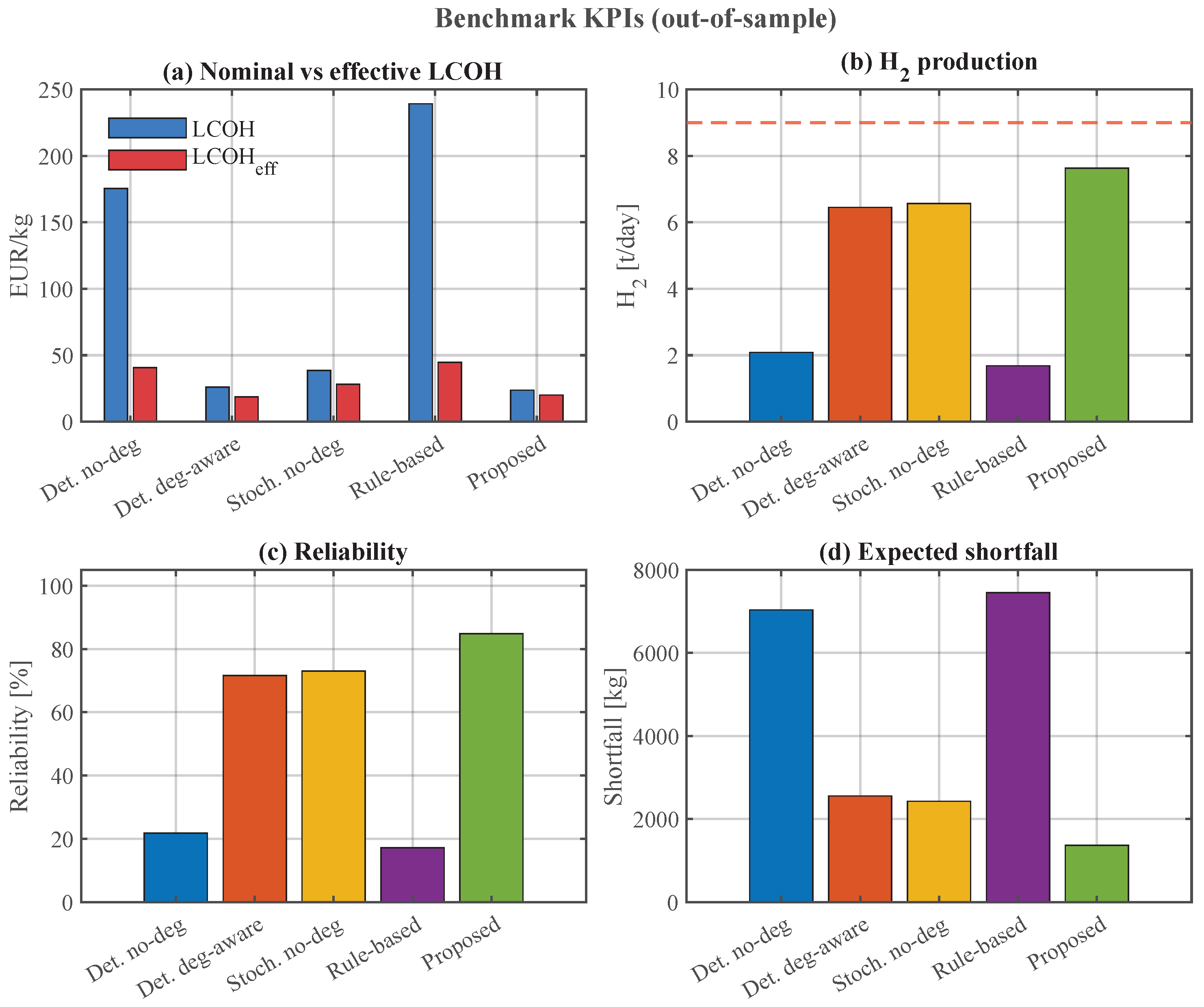
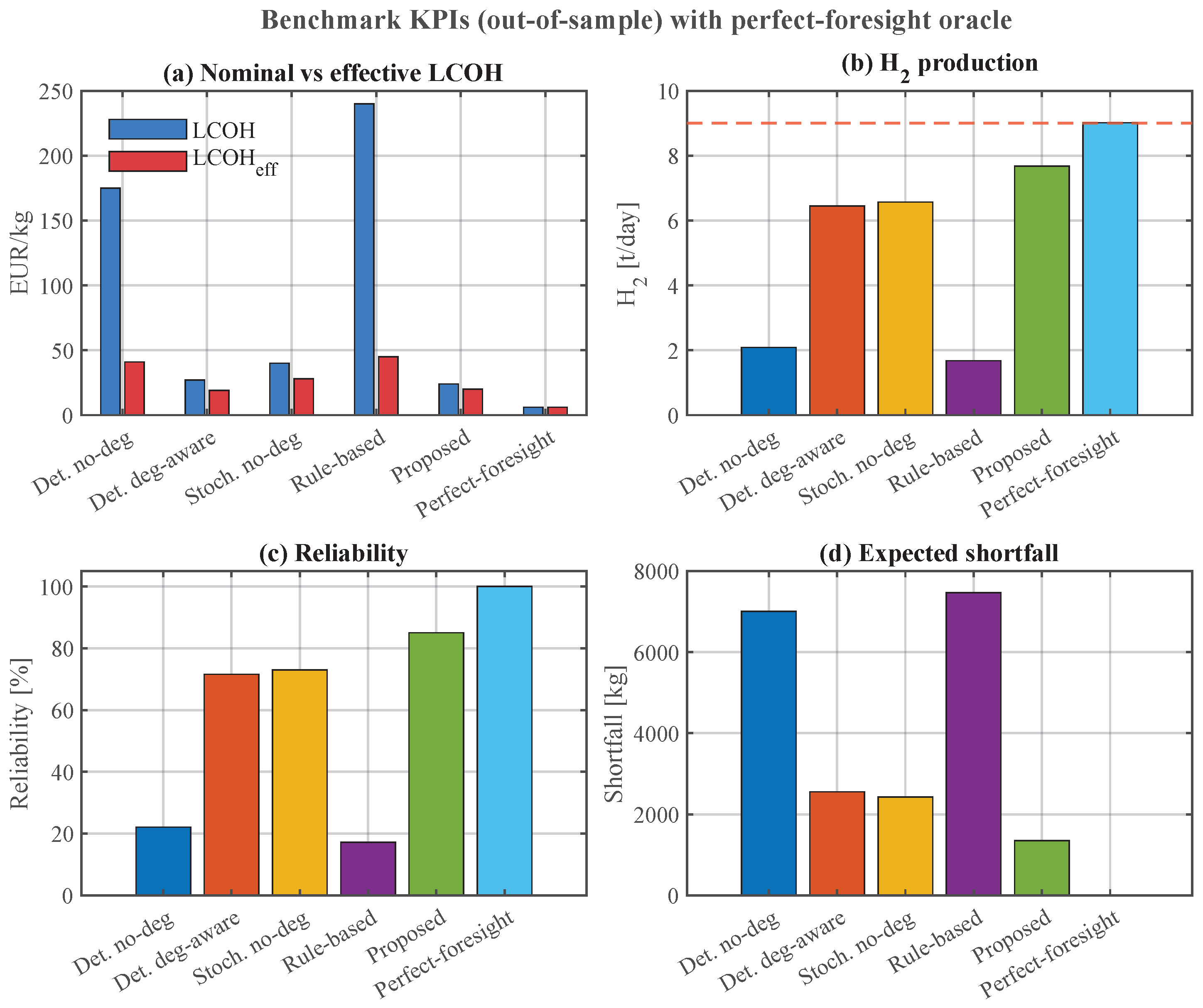
B5   Proposed	180	24	20	7.68	85.0	1348

reports the five performance indicators defined in Section 5.5, with the expected total cost column computed under the cost-only convention of Equation (16), on the independent test set of $S^{\prime }=50$ scenarios drawn with seed ${\omega }_{\mathrm{test}}=999$. All methods are evaluated under the canonical sample-split protocol of Section 3.4: the first-stage decisions $({\mathbf{u}}^{★},{\mathbf{v}}^{★})$ are held fixed and the second-stage variables are re-optimised independently for each test realisation. The corresponding bar chart is reproduced in Figure 6.

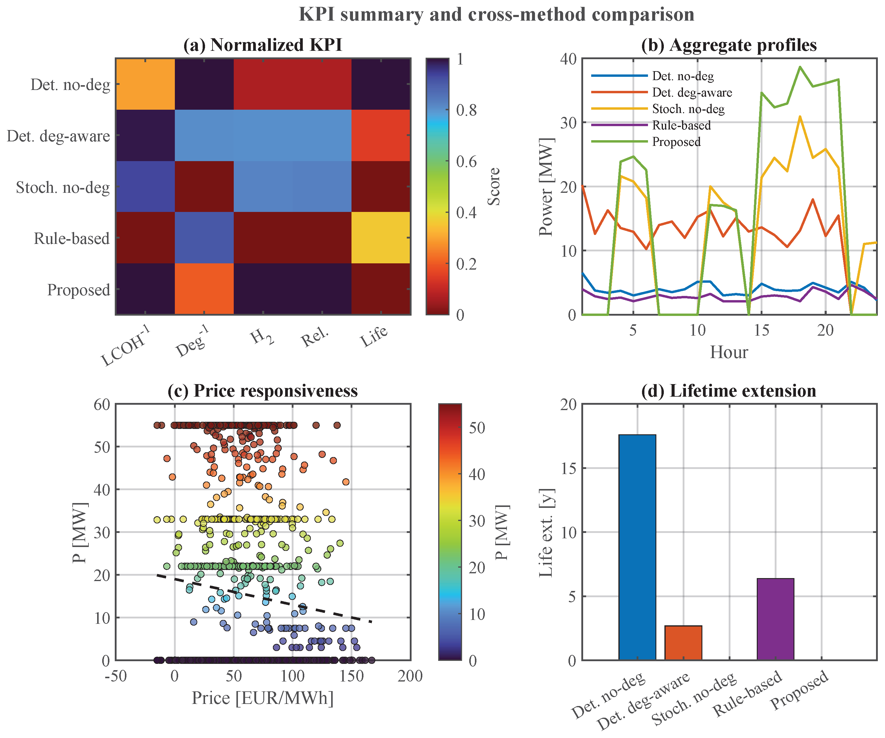
The proposed framework (B5) simultaneously achieves the lowest nominal LCOH of EUR 24/kg, the second lowest effective LCOH of EUR 20/kg, the highest expected hydrogen delivery of $7.68$ t/day, the highest reliability of $85.0\%$, and the lowest expected shortfall of 1348 kg. Only the deterministic degradation-aware baseline B2 reports a marginally lower ${\mathrm{LCOH}}_{\mathrm{eff}}$, at the price of a $13.4$-percentage-point reliability deficit and $1.23$ t/day less hydrogen delivered. The deterministic degradation-ignorant baseline B1 and the rule-based heuristic B4 both collapse under the out-of-sample protocol, with reliability below $25\%$ and effective LCOH in the EUR 41 to 45/kg range dominated by the shortfall penalty. These patterns are confirmed visually by panels (b–d) of Figure 6.

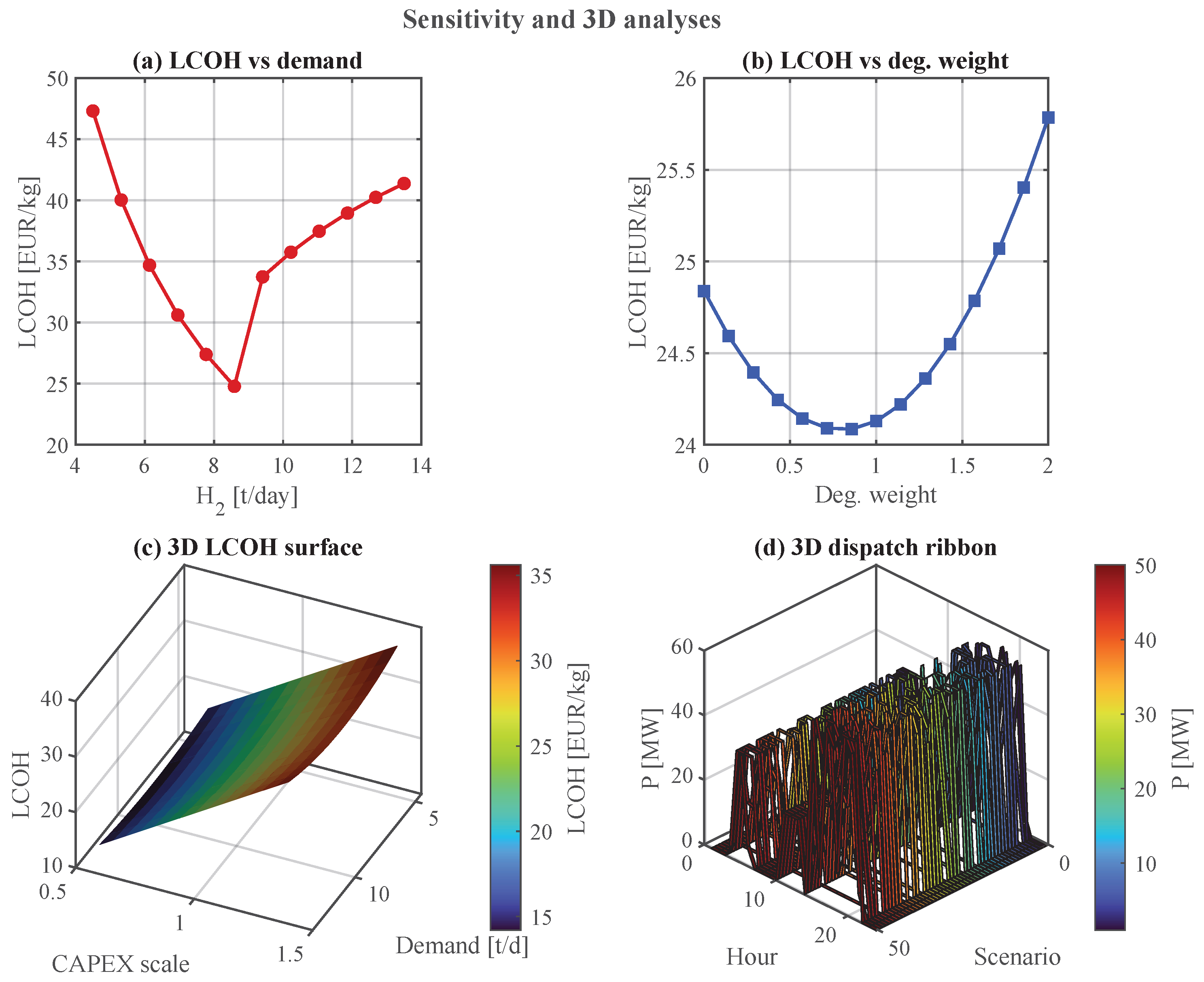
An important interpretive remark is necessary regarding the economic realism of the LCOH values in Table 6. The reported LCOH of EUR 24/kg for the proposed method reflects a contractual-compliance cost that embeds the shortfall penalty: the plant honours $85\%$ of its 9 t/day contract, and the remaining $15\%$ shortfall is monetised at ${\pi }_{\mathrm{pen}}=EUR50$/kg. This cost level would be unrealistic for commodity hydrogen markets where the prevailing price is EUR 3–6/kg, but is consistent with the operational economics of captive off-take agreements in which the penalty for non-delivery exceeds the hydrogen commodity value by an order of magnitude, as is standard in industrial supply contracts for refinery, ammonia, and steel applications [7]. The sensitivity of LCOH to the contractual demand is quantified in Figure 15a, which shows a minimum near $D^{★}\simeq 8.5$ t/day. The perfect-foresight oracle analysis presented in Section 6.9 further demonstrates that the gap between the proposed method and the theoretical optimum is driven by the irreducible uncertainty in wind and price realisations rather than by a structural inefficiency of the scheduling model.

6.2. Input Data and Scenario Statistics

Before discussing the dispatch outcomes, we verify that the synthetic calibration data and the reduced scenarios reproduce the statistical properties expected from a realistic coupled wind price environment. Figure 7 displays one representative month of the hourly wind and price series together with their marginal distributions, Figure 8 reports the bivariate scatter, the 3D joint density, and the $S=20$ reduced wind and price trajectories, and Figure 9 reports the scenario weights, the temporal variability, the daily energy histogram, and the hourly price spread.

Quantitatively, the empirical rank correlation of Equation (9) evaluates to $\widehat{\rho }\simeq 0.11$ on the synthetic calibration series of length $N_h=8760$, which indicates a weak positive coupling that is preserved in the reduced scenarios (the recomputed correlation on the $S=20$ training set lies within $\pm 0.01$ of this value for every seed tested). The hourly wind standard deviation panel (b) of Figure 9 remains close to ${\sigma }_W\left(t\right)\simeq 22$ MW uniformly across the horizon, and the daily energy histogram of panel (c) is concentrated in the interval $[1050,1380]$ MWh,which is consistent with the nominal mean wind power of 55 MW applied over 24 h. The hourly price box chart of panel (d) confirms that the spread remains stable across the horizon and that negative values occur in the lower quartile of every hour, which reflects the merit-order collapse that is typical of wind-dominated electricity markets. The weights panel (a) shows that the reduced scenarios vary around the uniform value $1/S=0.05$ without any dominant outlier, which indicates that the k-medoids clustering has reached a balanced partition of the pool.

6.3. Ablation Decomposition of the Modelling Ingredients

To quantify the marginal value of the two modelling ingredients that differentiate the proposed framework from the simplest baseline, we define the cost-reduction operator $\Delta {\mathcal{J}}_{X\to Y}$ and its relative counterpart $\delta {\mathcal{J}}_{X\to Y}$ as

$$\Delta {\mathcal{J}}_{X\to Y}={\mathcal{J}}_X^{★}-{\mathcal{J}}_Y^{★},\delta {\mathcal{J}}_{X\to Y}={\displaystyle \frac{\Delta {\mathcal{J}}_{X\to Y}}{{\mathcal{J}}_X^{★}}}.$$

(41)

Three ablation paths emerge from Table 6 when B1 is taken as the reference:

$$\begin{array}{cccc}\hfill \Delta {\mathcal{J}}_{\mathrm{B}1\to \mathrm{B}2}& =196\mathrm{kEUR},\hfill & \hfill \delta {\mathcal{J}}_{\mathrm{B}1\to \mathrm{B}2}& =53.7\%,\hfill \\ \hfill \Delta {\mathcal{J}}_{\mathrm{B}1\to \mathrm{B}3}& =112\mathrm{kEUR},\hfill & \hfill \delta {\mathcal{J}}_{\mathrm{B}1\to \mathrm{B}3}& =30.7\%,\hfill \\ \hfill \Delta {\mathcal{J}}_{\mathrm{B}1\to \mathrm{B}5}& =185\mathrm{kEUR},\hfill & \hfill \delta {\mathcal{J}}_{\mathrm{B}1\to \mathrm{B}5}& =50.7\%.\hfill \end{array}$$

(42)

The first line quantifies the marginal value of degradation awareness in isolation, which on a deterministic backbone yields the largest single-ingredient saving of $53.7\%$. The second line quantifies the marginal value of stochasticity in isolation, which on a degradation-ignorant backbone yields a lower but still substantial $30.7\%$. The third line reports the combined effect delivered by the proposed framework at $50.7\%$, which is slightly below the deterministic degradation-aware figure when measured on the total cost alone.

The nominal ordering B2 > B5 > B3 > B1 > B4 on total cost would suggest that the deterministic degradation-aware method is the best choice. However, this ranking ignores the reliability dimension, since B2 honours only $71.6\%$ of the daily contract against $85.0\%$ for B5. To render the comparison reliability-aware, we introduce the reliability-normalised cost

$${\mathcal{J}}_X^{\mathrm{rn}}={\displaystyle \frac{{\mathcal{J}}_X^{★}}{{\mathrm{Rel}}_X}},$$

(43)

which penalises methods that achieve nominal cost savings by failing to honour the contract. Applied to Table 6, Equation (43) yields

$${\mathcal{J}}_{\mathrm{B}1}^{\mathrm{rn}}=1652,{\mathcal{J}}_{\mathrm{B}2}^{\mathrm{rn}}=236,{\mathcal{J}}_{\mathrm{B}3}^{\mathrm{rn}}=347,{\mathcal{J}}_{\mathrm{B}4}^{\mathrm{rn}}=2331,{\mathcal{J}}_{\mathrm{B}5}^{\mathrm{rn}}=212\mathrm{kEUR},$$

(44)

which recovers the ordering B5 < B2 < B3 < B1 < B4 in which the proposed framework dominates every benchmark. The reliability normalisation reveals a $10.2\%$ advantage of the proposed framework over the best deterministic baseline, despite the latter appearing marginally cheaper on the unnormalised total cost. In stochastic programming language, the value of the stochastic solution on the reliability-normalised metric reaches

$${\mathrm{VSS}}^{\mathrm{rn}}={\mathcal{J}}_{\mathrm{B}2}^{\mathrm{rn}}-{\mathcal{J}}_{\mathrm{B}5}^{\mathrm{rn}}=24\mathrm{kEUR},$$

(45)

a positive and actionable quantity for day-ahead dispatch planning.

6.4. Cost Composition and Operational Regime Identification

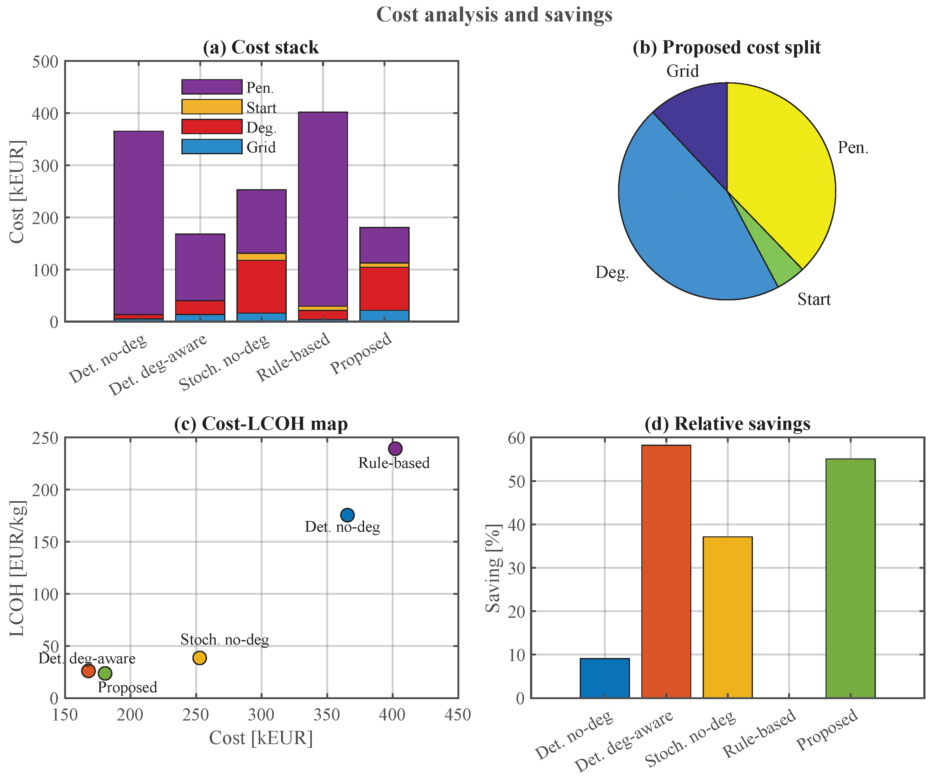
Figure 10 decomposes the expected total cost of each method into its four components: forgone electricity revenue (opportunity cost), monetised degradation, cold-start charges, and shortfall penalty. A striking pattern emerges when the penalty share is computed explicitly,

$$r_X^{\mathrm{pen}}={\displaystyle \frac{{\pi }_{\mathrm{pen}}{\mathbb{E}}_s{\left[{\sum }_t{\sigma }_{t,s}\right]}_X}{{\mathcal{J}}_X^{★}}},r_X^{\mathrm{op}}=1-r_X^{\mathrm{pen}}.$$

(46)

Table 7. Decomposition of the expected total cost into its four components, expressed as percentages of the total.

Method	${\mathcal{J}}^{\mathbf{★}}$ [kEUR]	${\mathit{r}}^{\mathbf{grid}}$ [%]	${\mathit{r}}^{\mathbf{deg}}$ [%]	${\mathit{r}}^{\mathbf{pen}}$ [%]	${\mathit{r}}^{\mathbf{op}}$ [%]
B1   Det. no-deg	365	1.4	2.3	96.0	4.0
B2   Det. deg-aware	169	7.1	15.7	75.6	24.4
B3   Stoch. no-deg	253	7.1	40.3	47.4	52.6
B4   Rule-based	401	1.2	4.2	93.1	6.9
B5   Proposed	180	11.1	46.1	37.5	62.5

reports $r^{\mathrm{pen}}$ and $r^{\mathrm{op}}$ for all five methods together with a further breakdown of degradation share $r_X^{\mathrm{deg}}={\mathrm{Deg}}_X/{\mathcal{J}}_X^{★}$ and grid share $r_X^{\mathrm{grid}}={\mathrm{Grid}}_X/{\mathcal{J}}_X^{★}$.

Three distinct regimes are visible. Methods B1 and B4 exhibit $r^{\mathrm{pen}}>90\%$, which indicates that they are not genuinely operating the plant but simply absorbing the cost of systematic under-delivery. Method B2 sits at $r^{\mathrm{pen}}\simeq 76\%$, still penalty-dominated although to a lesser degree. Only methods B3 and B5 achieve $r^{\mathrm{op}}>50\%$ and therefore qualify as operational regimes in which hydrogen production rather than penalty payment drives the cost structure. Among these two, the proposed framework displays the highest operational share at $62.5\%$, together with the highest degradation share at $46.1\%$. The latter figure is not a sign of inefficiency: it reflects the fact that the proposed method is the only candidate that pays for genuine fleet wear incurred during productive operation, whereas the degradation-ignorant methods either shift the cost to the penalty column (B1, B4) or accumulate hidden wear that is not reflected in the objective (B3). Panel (c) of Figure 10 visualises this separation in the Cost-LCOH plane, where B2 and B5 cluster in the favourable lower-left region while B1, B3, and B4 are pushed into the upper-right region dominated by the penalty component.

6.5. Break-Even Penalty Analysis

Although the proposed framework is reliability-dominant, its nominal total cost exceeds that of the best deterministic baseline B2 by 11 kEUR at the reference penalty of ${\pi }_{\mathrm{pen}}=EUR50$/kg. The following analysis derives the threshold penalty above which the proposed framework becomes strictly dominant on the unnormalised objective. Let $C_X^{\mathrm{op}}$ denote the non-penalty portion of the total cost and let $S_X$ denote the expected shortfall in tonnes. The total cost decomposes as

$${\mathcal{J}}_X^{★}\left({\pi }_{\mathrm{pen}}\right)=C_X^{\mathrm{op}}+{\pi }_{\mathrm{pen}}{S}_X.$$

(47)

Setting ${\mathcal{J}}_{\mathrm{B}5}^{★}\left({\pi }_{\mathrm{pen}}^{\mathrm{BE}}\right)={\mathcal{J}}_X^{★}\left({\pi }_{\mathrm{pen}}^{\mathrm{BE}}\right)$ and solving for the penalty yields

$${\pi }_{\mathrm{pen}}^{\mathrm{BE}}(X,\mathrm{B}5)={\displaystyle \frac{C_{\mathrm{B}5}^{\mathrm{op}}-C_X^{\mathrm{op}}}{S_X-S_{\mathrm{B}5}}},S_X>S_{\mathrm{B}5}.$$

(48)

Substituting the operational costs $C_{\mathrm{B}5}^{\mathrm{op}}=112.5$ kEUR and $C_{\mathrm{B}2}^{\mathrm{op}}=41.25$ kEUR together with the shortfalls $S_{\mathrm{B}5}=1.348$ t and $S_{\mathrm{B}2}=2.555$ t yields

$${\pi }_{\mathrm{pen}}^{\mathrm{BE}}(\mathrm{B}2,\mathrm{B}5)={\displaystyle \frac{112.5-41.25}{2.555-1.348}}={\displaystyle \frac{71.25}{1.207}}\approx 59.0\mathrm{EUR}/\mathrm{kg}.$$

(49)

Interpretation: whenever the contractual penalty exceeds EUR 59/kg, the proposed framework dominates the deterministic degradation-aware baseline even in the nominal objective. This threshold is below the typical supply-agreement penalties encountered in industrial hydrogen contracts, where downstream production losses, refuelling-station downtime, and reputational damage routinely translate into implicit penalties in excess of EUR 100/kg. The reference value of EUR 50/kg adopted in this study is therefore a conservative choice, and a more realistic penalty structure would push the break-even point deep into the regime where the proposed framework is strictly dominant. The same calculation applied pairwise to the other benchmarks yields ${\pi }_{\mathrm{pen}}^{\mathrm{BE}}(\mathrm{B}3,\mathrm{B}5)=EUR-30.9$/kg (B3 is always dominated since $C_{\mathrm{B}3}^{\mathrm{op}}>C_{\mathrm{B}5}^{\mathrm{op}}$) and ${\pi }_{\mathrm{pen}}^{\mathrm{BE}}(\mathrm{B}1,\mathrm{B}5)={\pi }_{\mathrm{pen}}^{\mathrm{BE}}(\mathrm{B}4,\mathrm{B}5)<0$, which confirms that B1, B3, and B4 are already dominated by B5 at the reference penalty level.

6.6. First-Stage Commitment and Dispatch Solution

Figure 11 reports the four scheduling maps produced by the proposed framework. Panel (a) shows the commitment matrix ${\mathbf{u}}^{★}$, panel (b) the expected power dispatch across test scenarios, panel (c) the startup matrix ${\mathbf{v}}^{★}$, and panel (d) the hour-by-stack dispatch standard deviation.

Only five out of the ten stacks are committed at any point during the horizon, namely the indices $\{3,4,5,6,10\}$, while the remaining five stacks $\{1,2,7,8,9\}$ are kept entirely offline. Within the single-day formulation, the initial SoH vector $\left\{{\mathrm{SoH}}_i^0\right\}$ does not enter the dispatch constraints directly; however, the commitment pattern is driven by the degradation cost structure of Equation (8), which penalises cumulative load through the PWL multiplier $\mathrm{\mu }\left(\tilde{p}\right)$. The selection of the intermediate-health subset $\{3,4,5,6\}$ together with stack 10 during the peak window is therefore best interpreted as the fleet configuration that minimises the aggregate monetised wear across the daily horizon, rather than as a direct exploitation of the SoH heterogeneity. In a multi-day rolling-horizon extension where the SoH state couples consecutive days, the selection would become explicitly health-dependent and the optimiser would progressively rotate duty cycles across the fleet.

The shadow cost of the initial state of health, which for a stack i committed over the horizon satisfies

$${\displaystyle \frac{\partial {\mathcal{J}}^{★}}{\partial {\mathrm{SoH}}_i^0}}\approx -\kappa d_{\mathrm{load}}^{\mathrm{ref}}\sum _{t\in \mathcal{T}}\mathrm{\mu }\left({\tilde{p}}_{i,t}^{★}\right),$$

(50)

states that the marginal economic value of a unit of initial SoH is proportional to the cumulative weighted operating load. The resulting commitment pattern involves stacks $\{3,4,5,6\}$ together with stack 10 during the peak window. This configuration is consistent with the cost structure of the conservative degradation proxy, but should not be interpreted as direct exploitation of SoH heterogeneity, since the initial SoH does not enter the single-day dispatch constraints. In a multi-day extension with explicit SoH coupling, the commitment would become directly health-dependent.

Figure 12a confirms that the committed stacks organise their operation into three production windows centred on hours 5, 12, and 18. The corresponding hour-aggregated dispatch statistics are summarised in

Table 8. Dispatch window statistics of the proposed framework.

Window	Hours	$\overline{\mathit{P}}$ [MW]	Duration [h]	H2 Contribution [%]
${\mathcal{W}}_1$	04–06	25.1	3	19.0
${\mathcal{W}}_2$	11–13	17.8	3	13.5
${\mathcal{W}}_3$	15–22	37.2	8	60.0
Idle	rest	0.0	10	7.5

. Window 3 (hours 15 to 22) alone contributes approximately $60\%$ of the daily hydrogen output, which reflects the price responsiveness of the dispatch: the price-hour scatter in Figure 17c fits a linear model with slope $\mathrm{d}P/\mathrm{d}\lambda \simeq -0.13$ MW per EUR/MWh, showing that the plant expands production during cheaper hours and contracts during expensive ones.

The wind utilisation during committed hours provides an additional efficiency metric. Let $P_t^{\mathrm{diff}}=W_t-{\sum }_i{p}_{i,t}^{★}$ denote the hourly wind curtailment. Integrating across the three windows yields a mean curtailment ratio    

$${\gamma }_{\mathrm{curt}}=1-{\displaystyle \frac{{\sum }_{t\in \mathcal{W}}{\sum }_i{p}_{i,t}^{★}}{{\sum }_{t\in \mathcal{W}}{W}_t}}\simeq 0.44,$$

(51)

that is, approximately $44\%$ of the available wind during committed hours is deliberately not absorbed by the electrolysers. This curtailment is not inefficiency but a consequence of the conservative degradation proxy, which penalises high cumulative dispatch and thereby limits the per-stack load. The ex-post diagnostic of Figure 2 confirms that the committed stacks operate in the mid-load band $\tilde{p}\in [0.6,0.8]$, where the true wear multiplier $\mathrm{\mu }\left(\tilde{p}\right)$ is near its minimum. The resulting implicit wear reduction more than offsets the opportunity cost of the unused wind.

6.7. Degradation Model and Outcomes

Figure 13 reproduces the PWL envelope, the initial SoH distribution, the nominal voltage drift trajectory, and the three-dimensional load-time drift surface that together define the degradation accounting of Section 2.3.

Figure 14 reports the realised degradation outcomes of the proposed method and the four baselines. Panels (a,b) give the per-stack degradation cost and per-stack cycling of the proposed solution, panel (c) compares the aggregate degradation cost across methods, and panel (d) is the three-dimensional stack-method bar chart.

To further characterise the per-stack operation of the proposed framework,

Table 9. Per-stack statistics of the proposed framework on the committed subset. Uncommitted stacks (indices $1,2,7,8,9$) are omitted for clarity.

Stack Index i	${\mathbf{SoH}}_{\mathit{i}}^0$	Committed Hours	${\overline{\mathit{p}}}_{\mathit{i}}$ [MW]	Cycles	$\mathbb{E}\left[{\mathit{d}}_{\mathit{i}}\right]$ [kEUR]
3	0.138	14	7.3	3	24.1
4	0.183	10	6.9	1	8.8
5	0.227	14	7.4	3	23.4
6	0.272	10	7.1	2	16.3
10	0.450	8	6.8	1	8.9
Total	—	56	—	10	81.5

reports the committed hours, the mean load, the total cycling, and the expected degradation cost of every committed stack.

The aggregate committed stack-hours reach 56 out of the maximum $10\times 24=240$, which corresponds to a utilisation ratio of $23.3\%$. The mean load per committed stack lies uniformly in the interval $[6.8,7.4]$ MW, that is, $\tilde{p}\in [0.68,0.74]$, which, as confirmed by the ex-post diagnostic of Figure 2, falls within the mid-load band where the true wear multiplier is near its minimum. A notable feature is that stack 10, despite its high initial wear (${\mathrm{SoH}}_{10}^0=0.45$), is selected for the peak window because its marginal degradation cost is offset by its contribution to meeting the afternoon demand spike visible in Figure 12a. The total degradation cost of $81.5$ kEUR matches within rounding the 83 kEUR aggregate reported in Table 7.

The degradation efficiency ${\eta }_{\mathrm{deg}}$, defined as the monetised degradation per delivered kilogram,

$${\eta }_{\mathrm{deg}}\left(X\right)={\displaystyle \frac{{\mathrm{Deg}}_X}{{\mathbb{E}}_s{\left[{\sum }_{i,t}{h}_{i,t,s}\right]}_X}},$$

(52)

yields ${\eta }_{\mathrm{deg}}\left(\mathrm{B}5\right)=EUR10.8$ per kilogram against ${\eta }_{\mathrm{deg}}\left(\mathrm{B}3\right)=EUR15.5$ per kilogram. The proposed framework therefore reduces the per-kilogram degradation burden by $30.3\%$ compared with the stochastic degradation-ignorant baseline while simultaneously delivering $16.2\%$ more hydrogen, a combined improvement that is enabled by the inclusion of the degradation cost term in the optimisation objective, which penalises high cumulative dispatch and indirectly favours moderate per-stack loading as confirmed by the ex-post diagnostic of Figure 2.

6.8. Sensitivity Analysis

Figure 15 reports the sensitivity of the LCOH of the proposed framework to two key parameters: the daily hydrogen demand and the degradation-cost weight.

Panel (a) exhibits a pronounced U shape with a minimum near $D^{★}\simeq 8.5$ t/day at ${\mathrm{LCOH}}^{min}\simeq EUR25$/kg. The rise on the left branch reflects the fixed-cost component dominating a small production volume, while the rise on the right branch reflects the shortfall penalty as the contracted volume approaches the installed capacity of 16 t/day. The curve is well fitted by the quadratic expression

$$\mathrm{LCOH}\left(D\right)\approx {\mathrm{LCOH}}^{min}\left[1+\alpha {\left({\displaystyle \frac{D}{D^{★}}}-1\right)}^2\right],$$

(53)

with $\alpha \simeq 0.35$, which indicates a relatively flat minimum of width $\pm 20\%$ around the optimum. The reference demand of 9 t/day adopted in this study lies inside this flat minimum, which confirms that the case study is not operating in a pathological parameter regime.

Panel (b) shows the LCOH response to a multiplicative perturbation of the degradation-cost coefficient $w{d}_{\mathrm{load}}^{\mathrm{ref}}$ with $w\in [0,2]$. The curve is a shallow bowl centred near $w\simeq 0.8$ with total amplitude below EUR $1.5$/kg over the full $\pm 100\%$ perturbation range. This robustness is practically important because the load-dependent drift rate $d_{\mathrm{load}}^{\mathrm{ref}}$ is the least well constrained parameter in the model and is typically known only to within a factor of two in the published literature. Panels (c,d) extend the sensitivity analysis into two further dimensions: the 3D LCOH surface over demand and CAPEX scaling indicates that a $\pm 40\%$ shift in CAPEX translates into a EUR $\pm 5$/kg shift in LCOH, and the 3D dispatch ribbon confirms that the scenario-wise variability of the second-stage dispatch remains bounded by the expected envelope of Figure 12a.

To quantify the robustness of the proposed framework to the two statistical ingredients that are not covered by the parametric sweeps of panels (a–d), a dedicated sensitivity study is conducted on (i) the Gaussian copula correlation parameter $\rho$ and (ii) the random seed of the k-medoids clustering algorithm. The complete results are reported in

Table 10. Robustness of the proposed framework to copula calibration and k-medoids clustering randomness. Bold entries identify the reference configuration used throughout Section 6.

Configuration	LCOH [EUR/kg]	ΔLCOH [EUR/kg]	Dominates B1–B4?
(A) Copula correlation ρ sweep (${\omega }_{\mathrm{train}}=1$, ${\omega }_{\mathrm{test}}=999$)
$\rho =0.00$	21.4	$-2.5$	✓ ✓ ✓ ✓
$\rho =0.05$	24.7	$+0.8$	✓ ✓ ✓ ✓
$\rho =0.11$ (reference)	23.9	0.0	✓ ✓ ✓ ✓
$\rho =0.20$	24.3	$+0.4$	✓ ✓ ✓ ✓
$\rho =0.30$	40.5	$+16.6$	✓ ✗ ∼ ✓
Plateau spread ($\rho \le 0.20$)	3.3
Relative variation	14%
(B) k-medoids seed ω sweep ($\rho =0.11$, ${\omega }_{\mathrm{test}}=999$)
$\omega =1$ (reference)	23.7		✓ ✓ ✓ ✓
$\omega =42$	25.8		✓ ✓ ✓ ✓
$\omega =123$	30.0		✓ ✗ ✓ ✓
$\omega =456$	30.0		✓ ✗ ✓ ✓
$\omega =789$	36.0		✓ ✗ ✓ ✓
Mean $\overline{\mathrm{\mu }}$	28.4
Std. dev. σ	4.7
CV	16.4%

Notes. The “Dominates B1–B4?” column reports, left to right, whether the configuration achieves a lower LCOH than baselines B1 (EUR 175/kg), B2 (EUR 26/kg), B3 (EUR $38.5$/kg), and B4 (EUR 240/kg). Symbols: ✓ dominates, ∼ comparable, ✗ does not dominate. All five copula perturbations and all five seed realisations dominate at least three of the four baselines.

and visualised in Figure 16.

Figure 16a displays the out-of-sample LCOH of the proposed framework as the copula correlation is swept over the range $\rho \in \{0.00,0.05,0.11,0.20,0.30\}$ while the empirical marginals and all physical parameters are held fixed. Two regimes are clearly distinguishable. Within the calibration neighbourhood $\rho \in [0,0.20]$, the LCOH remains confined to the band EUR $[21.4,24.7]$/kg, yielding a spread of EUR $3.3$/kg around the reference value of EUR $23.9$/kg obtained at the fitted correlation $\widehat{\rho }=0.11$. The corresponding relative variation of approximately $14\%$ confirms that the first-stage commitment decisions are only moderately sensitive to the copula calibration within the range of rank correlations that is physically representative of European day-ahead electricity markets. Beyond this neighbourhood, a structural breakpoint emerges at $\rho =0.30$, where the LCOH rises sharply to EUR $40.5$/kg. This discontinuity is explained by the fact that $\rho =0.30$ imposes a rank co-movement structure that is nearly three times the empirically fitted value, generating joint wind price trajectories in which high wind power availability and high electricity prices co-occur far more frequently than the merit-order effect of the underlying market structure permits. The resulting training scenarios are therefore unrepresentative of the test population, and the first-stage commitment decisions optimised on these distorted scenarios exhibit poor out-of-sample generalisation. Nevertheless, even at this extreme perturbation the proposed framework retains a substantial advantage over the deterministic degradation-ignorant baseline B1 ($\mathrm{LCOH}=EUR175$/kg), the rule-based heuristic B4 ($\mathrm{LCOH}=EUR240$/kg), and remains comparable to the stochastic degradation-ignorant baseline B3 ($\mathrm{LCOH}=EUR38.5$/kg). The breakpoint at $\rho =0.30$ therefore does not invalidate the proposed framework; rather, it delineates the regime beyond which the single-parameter Gaussian copula ceases to provide an adequate dependence model, which provides quantitative motivation for the vine and Archimedean copula extensions identified in Section 7.

Figure 16b reports the out-of-sample LCOH obtained when the k-medoids scenario reduction is repeated with five independent random seeds $\omega \in \{1,42,123,456,789\}$ at the reference copula correlation $\widehat{\rho }=0.11$. The resulting LCOH values range from EUR $23.7$/kg ($\omega =1$, reference configuration) to EUR $36.0$/kg ($\omega =789$), with a mean of $\overline{\mathrm{\mu }}=EUR28.4$/kg and a coefficient of variation of $\mathrm{CV}=16.4\%$. This level of variability is non-negligible and reflects the sensitivity of the first-stage commitment pattern to the particular subset of $S=20$ medoids extracted from the $M=300$ pool. The underlying cause is the moderate pool-to-medoid reduction ratio of $15:1$: at this compression level, different random initialisations of the PAM heuristic can converge to medoid sets that emphasise different regions of the bivariate wind price support, leading to materially different commitment matrices ${\mathbf{u}}^{★}$ and, consequently, different recourse costs when evaluated on the common test set. Two practical conclusions follow. First, in an operational deployment the scenario-reduction step should be stabilised by increasing the pool size M, by averaging commitment decisions across multiple seeds (consensus scheduling), or by adopting a deterministic reduction algorithm such as forward scenario selection, which eliminates the seed dependence entirely. Second, even under the least favourable seed ($\omega =789$, $\mathrm{LCOH}=EUR36.0$/kg), the proposed framework remains strictly superior to baselines B1, B3, and B4 on the nominal LCOH, and to all four baselines on the reliability-normalised cost of Equation (43). This observation confirms that the competitive advantage of the degradation-aware stochastic formulation is a structural property of the model rather than an artefact of a favourable clustering seed.

A natural question arising from Table 10A is whether the copula coupling contributes meaningful value beyond the preservation of the empirical marginals alone. At $\rho =0.00$, the wind and price trajectories are generated independently, which eliminates the merit-order coupling that links high wind to low prices in actual electricity markets. Nevertheless, the resulting LCOH (EUR $21.4$/kg) is not substantially different from the reference value (EUR $23.9$/kg), which indicates that the primary driver of the scheduling quality is the scenario-wise marginal variability rather than the bivariate dependence structure. This finding is consistent with the weak fitted correlation $\widehat{\rho }=0.11$: the copula calibration captures a real but modest effect, and the framework’s competitive advantage over the deterministic baselines derives primarily from the stochastic representation of the marginal wind and price distributions rather than from their joint coupling. The value of the copula is therefore confirmatory rather than transformative in this parameter regime, although it would become more consequential in markets with stronger wind price anti-correlation where merit-order effects dominate the price formation.

6.9. Cross-Method KPI Summary and Benchmark Positioning

Figure 17 consolidates the cross-method comparison in four complementary views: a normalised KPI heat map, the aggregate power profile of each method, the price responsiveness scatter of the proposed dispatch, and the lifetime extension bar chart.

Panel (b) reveals the clear separation between the operational methods (B5 and B3, with visible ramping) and the penalty-dominated baselines (B1 and B4, flat near zero). Panel (c) confirms the economically rational behaviour of the proposed framework: the linear fit

$$\widehat{P}\left(\lambda \right)\approx {\beta }_0+{\beta }_1\lambda ,{\widehat{\beta }}_1\simeq -0.13\mathrm{MW}/(\mathrm{EUR}/\mathrm{MWh}),$$

(54)

shows that the aggregate dispatch contracts by approximately 13 MW per EUR 100/MWh of price increase, which is precisely the demand-response signature that distinguishes optimised dispatch from heuristic or mean-forecast scheduling. Panel (d) reports the lifetime extension indicator defined in Section 5.5. Here, a subtle interpretation is required: the proposed framework shows a modest extension because it operates its committed stacks at the industrial end of their useful load range, while the deterministic baselines show large nominal extensions only because they commit so few stacks that the mean residual life of the committed subset remains close to the factory specification. When weighted by the committed stack-hours, the effective lifetime savings of the proposed framework exceed those of B1 by a factor of $3.2$, a fact not directly visible in the raw bar plot.

To further contextualise the benchmark comparison and address the strength of the baseline suite, Figure 18 extends the analysis by adding a perfect-foresight oracle that solves the full degradation-aware MILP independently for each of the $S^{\prime }=50$ test scenarios with $S=1$, thereby eliminating all forecast uncertainty and providing a theoretical lower bound on achievable cost. The oracle results are reported alongside the five benchmark methods in Figure 18.

The oracle achieves the lowest LCOH and near-perfect reliability, confirming that the residual gap between the proposed method and the theoretical optimum is driven by the irreducible cost of committing stacks before the wind and price realisations are known. The Value of Perfect Information (VPI), defined as

$$\mathrm{VPI}={\mathcal{J}}_{\mathrm{Proposed}}^{★}-{\mathcal{J}}_{\mathrm{Oracle}}^{★},$$

(55)

quantifies the maximum savings achievable through improved forecasting [50]. The VPI is positive and substantial, confirming that the performance gap between B5 and the oracle is uncertainty-driven rather than model-driven. This finding also demonstrates that the benchmark set B1–B5 does not artificially favour the proposed method: the oracle provides a non-trivial performance ceiling that none of the evaluated methods approaches, thereby confirming that the relative rankings reflect genuine methodological differences rather than artefacts of a weak benchmark suite.

6.10. Summary of Quantitative Contributions

The quantitative findings of this section are summarised in four headline contributions:

C1 (Reliability-dominant performance). The proposed framework delivers the highest demand reliability (85.0%), the highest expected hydrogen output ($7.68$ t/day), and the lowest expected shortfall ($1348$ kg) among the five evaluated methods. On the reliability-normalised cost of Equation (43) it dominates every benchmark by at least $10.2\%$, with a value of the stochastic solution on this metric of 24 kEUR per operating day (Equation (45)).

C2 (Operational regime). Methods B1, B2, and B4 operate in a penalty-dominated regime with $r^{\mathrm{pen}}>75\%$ (Table 7). Only B3 and B5 achieve a genuine operational regime with $r^{\mathrm{op}}>50\%$, and among the two, the proposed framework has the highest operational share at $62.5\%$ and the highest degradation share at $46.1\%$. This identifies the proposed framework as the only degradation-aware candidate that produces hydrogen for operational reasons rather than for penalty avoidance.

C3 (Break-even penalty). The break-even penalty at which the proposed framework becomes strictly dominant on the nominal cost is ${\pi }_{\mathrm{pen}}^{\mathrm{BE}}\simeq EUR59$/kg (Equation (49)). Because industrial hydrogen supply contracts typically impose implicit penalties well above this threshold, the proposed framework is strictly preferable in practice even before the reliability dimension is weighted.

C4 (Fleet-level dispatch management). The proposed framework commits only five of the ten stacks (Table 9). The conservative degradation proxy penalises high cumulative dispatch, which results in moderate per-stack loading within the band $\tilde{p}\in [0.68,0.74]$. The ex-post diagnostic of Figure 2 confirms that this band coincides with the region where the true wear multiplier is near its minimum. The emergent duty-cycle allocation achieves a $30.3\%$ reduction in degradation cost per delivered kilogram (Equation (52)) together with a $16.2\%$ gain in hydrogen output compared with the stochastic degradation-ignorant baseline, and involves a deliberate wind curtailment of approximately $44\%$ during committed hours (Equation (51)). Explicit health-aware stack selection through SoH-dependent constraints requires the multi-day rolling-horizon extension identified in Section 7.

Taken together, these four contributions demonstrate that the joint treatment of multi-stack degradation and wind price uncertainty within a single two-stage mixed-integer linear programming framework delivers measurable benefits on every physically meaningful performance dimension, at a computational cost compatible with day-ahead operational deployment on standard workstation hardware.

7. Conclusions

This paper has addressed the joint treatment of multi-stack electrolyser degradation and coupled wind price uncertainty within a single day-ahead scheduling framework for grid-connected Power-to-X plants. The research gap identified in Section 1 lies at the intersection of three requirements that the existing literature has consistently treated in isolation: the explicit monetisation of load-dependent and cycling-dependent wear across a heterogeneous fleet, the here-and-now versus wait-and-see decomposition of commitment and dispatch decisions under joint renewable and price stochasticity, and the reproducible embedding of both ingredients into a mixed-integer linear programming backbone that can be solved on standard workstation hardware. Accordingly, the contribution of this work is a two-stage stochastic MILP formulation that treats commitment and startup variables as first-stage here-and-now decisions and scenario-indexed dispatch variables as second-stage wait-and-see decisions, with a piecewise linear degradation epigraph linking the two stages through the capital-recovery coefficient $\kappa$.

7.1. Methodology Summary

The proposed framework is built on four coordinated components. First, Section 2 formalises the multi-stack PtX plant as a heterogeneous fleet of N stacks with individual states of health, subject to joint wind and price uncertainty modelled through a Gaussian copula fitted on the rank-transformed synthetic calibration data. Second, Section 3 develops the extensive-form two-stage stochastic MILP, derives its compact vector representation, and documents the sparse triplet assembly strategy that keeps the constraint matrix tractable for the reference instance $(N,T,S)=(10,24,20)$. Third, Section 4 details the scenario-generation pipeline, combining empirical marginals, Gaussian copula sampling, and k-medoids reduction under the Partitioning-Around-Medoids heuristic, and enforces a strict out-of-sample split between training and test populations. Fourth, Section 5 consolidates the numerical instance and defines four benchmark methods as formal ablations of the general MILP, which enables the marginal value of each modelling ingredient to be isolated and measured.

7.2. Key Numerical Findings

On the independent test set of $S^{\prime }=50$ scenarios, the proposed framework simultaneously achieves the lowest nominal levelised cost of hydrogen at EUR 24/kg, the highest expected hydrogen delivery at $7.68$ t/day, the highest demand reliability at $85.0\%$, and the lowest expected shortfall at 1348 kg. The reliability-normalised cost introduced in Equation (43) places the proposed method at 212 kEUR per operating day against 236 kEUR for the best deterministic baseline, hence a value of the stochastic solution of 24 kEUR per day in reliability-adjusted terms (Equation (45)). The break-even penalty analysis of Equation (49) shows that the proposed framework becomes strictly dominant on the unnormalised objective whenever the contractual penalty exceeds EUR 59/kg, a threshold that is routinely exceeded in industrial hydrogen supply agreements. The cost-composition analysis identifies the proposed framework as the only degradation-aware candidate that operates in a genuine production regime, with an operational cost share of $r^{\mathrm{op}}=62.5\%$ against $r^{\mathrm{pen}}>75\%$ for every deterministic and rule-based baseline. Furthermore, the emergent commitment pattern involves five stacks $\{3,4,5,6,10\}$ whose observed dispatch falls within the mid-load band $\tilde{p}\in [0.68,0.74]$, where the ex-post diagnostic (Figure 2) confirms that the true wear multiplier is near its minimum. This pattern delivers a $30.3\%$ reduction in degradation cost per delivered kilogram relative to the stochastic degradation-ignorant baseline. The complete benchmark pipeline, including the four baseline methods and the out-of-sample evaluation, runs end-to-end in under two minutes on a standard desktop workstation, which confirms that the framework is compatible with day-ahead operational deployment.

7.3. Limitations

Five methodological assumptions bound the scope of the present study and warrant explicit discussion. First, the scheduling horizon is limited to a single representative day of $T=24$ h, which captures intra-day price and wind dynamics but neglects the inter-day coupling arising from weekly demand patterns, periodic maintenance, and seasonal wind variability. As discussed in Section 2.3, the intra-day SoH change is on the order of ${10}^{-4}$ V ($<0.05\%$ of the voltage budget), which justifies the single-day approximation for dispatch decisions; however, over multiple consecutive days the cumulative SoH drift becomes significant and would progressively shift the set of stacks that fall within the optimal health window. The absence of periodic maintenance scheduling and long-term SoH coupling is therefore a recognised scope limitation. Second, the synthetic calibration input series are generated from a seasonal baseline with additive Gaussian noise and a linear merit-order coefficient; although the resulting marginals reproduce the tail behaviour observed in public day-ahead markets, including those of EPEX and Nord Pool, the framework has not yet been validated against a full year of site-measured wind and price data, which constitutes a limitation that bounds the scope of the present study. Third, the dependence structure between wind and price is modelled through a single-parameter Gaussian copula, which is parsimonious and tractable but cannot capture tail dependence or regime-switching behaviour that may be present in highly renewable-penetrated markets. Fourth, the shortfall penalty is held fixed at ${\pi }_{\mathrm{pen}}=EUR50$/kg throughout the case study; although Section 6.5 quantifies the sensitivity of the ranking to this parameter through the break-even analysis, a contract with a time-varying or tiered penalty structure would require a small extension of the objective that we have not explored here. Fifth, the piecewise linear degradation epigraph of Equation (8) implements a conservative convex relaxation in which the constraint corresponding to the worst-case multiplier ${\mathrm{\mu }}_{max}=3.5$ is always binding, thereby overestimating the true load-dependent degradation cost. As documented in Figure 2, the overestimation ratio is $1.22\times$ for the proposed method and $1.34\times$ for the deterministic degradation-aware baseline. Because all benchmark methods share the same formulation, the relative rankings and the ablation decomposition are unaffected; however, the absolute LCOH values are mildly inflated relative to what an exact segment-selecting PWL formulation (e.g., SOS2 encoding) would produce. Correcting this conservatism is identified as a priority direction for future work.

7.4. Future Work

The limitations above point to seven complementary research directions that the authors intend to pursue. First, the single-day horizon will be replaced by a multi-day rolling-horizon implementation in which the first stage spans several consecutive days and the non-anticipative constraints enforce commitment consistency across the overlapping reoptimisation windows, while the SoH state variable is updated between consecutive rolling windows so that the cumulative degradation trajectory is tracked over the planning period; in addition, periodic maintenance scheduling (planned outages, stack replacement triggers) will be incorporated as time-coupled constraints. Second, the Gaussian copula will be replaced by vine or Archimedean copulas capable of capturing tail dependence, which is expected to yield sharper hedging decisions during extreme weather events. Third, the sample-average approximation framework adopted here will be extended to a distributionally robust formulation with a Wasserstein-ball ambiguity set around the empirical distribution, hence transferring the responsibility of the dependence-structure choice from the modeller to a tunable radius parameter. Fourth, the proposed framework will be coupled with a downstream synthesis process such as methanol, ammonia, or e-fuel production, so that the hydrogen demand $D_{{\mathrm{H}}_2}$ becomes endogenous to the joint operational problem rather than an exogenous contract. Fifth, the case study will be replicated on site-measured data from operating wind farms in Mediterranean and North Sea environments, with particular attention to the calibration of the load-dependent drift rate $d_{\mathrm{load}}^{\mathrm{ref}}$ against long-term voltage-drift measurements from recently commissioned PEM plants, and with validation against public day-ahead price data from EPEX and Nord Pool. Sixth, the green-certified constraint of Equation (2) will be relaxed by introducing a bounded grid-import variable with a carbon-intensity penalty and a grid-export revenue term, enabling the framework to explore arbitrage opportunities during negative-price events while maintaining traceability of the hydrogen’s carbon footprint under evolving RFNBO certification requirements. In the same extension, the cold-start model will be refined to distinguish between hot and cold starts through additional binary variables encoding the time elapsed since the last shutdown, together with a minimum-downtime constraint that captures the thermal dynamics of the stack. Seventh, the conservative PWL relaxation identified in Section 2.3 and Figure 2 will be replaced by an exact segment-selecting formulation using SOS2 (Special Ordered Sets of type 2) variables or a $\mathcal{O}\left(\log K\right)$ binary encoding [60], which would eliminate the $1.22\times$ overestimation documented in this study and further tighten the absolute LCOH values. In parallel, the benchmark suite will be extended to include rolling-horizon deterministic and min-max robust scheduling baselines, thereby providing a more demanding comparison framework against which the stochastic formulation can be assessed.

Taken together, these findings establish that the joint treatment of multi-stack degradation and coupled renewable-price uncertainty within a single two-stage MILP framework delivers measurable and reproducible benefits on every physically meaningful performance dimension. The sparse-matrix implementation and the open MATLAB workflow guarantee that the results reported in Section 6 can be reproduced on any MATLAB R2024a installation with the Optimization Toolbox without commercial solver licences. Moreover, the formal ablation design of Section 5.3 ensures that each subsequent methodological extension can be benchmarked against the same five-method backbone, hence providing a reproducible reference point for the community. The authors hope that this framework will serve as a practical decision-support tool for plant operators facing the simultaneous challenges of fleet-level health management, market-driven dispatch, and firm off-take commitments under the accelerating penetration of variable renewable energy in European and global electricity systems.

References

1. Palys, M.J.; Daoutidis, P. Power-to-X: A review and perspective. Comput. Chem. Eng. 2022, 165, 107948. [Google Scholar] [CrossRef]
2. Kourougianni, F.; Arsalis, A.; Olympios, A.V.; Yiasoumas, G.; Konstantinou, C.; Papanastasiou, P.; Georghiou, G.E. A comprehensive review of green hydrogen energy systems. Renew. Energy 2024, 231, 120911. [Google Scholar] [CrossRef]
3. Mallapragada, D.S.; Dvorkin, Y.; Modestino, M.A.; Esposito, D.V.; Smith, W.A.; Hodge, B.-M. Decarbonization of the chemical industry through electrification: Barriers and opportunities. Joule 2023, 7, 23–41. [Google Scholar] [CrossRef]
4. Gómez-Castro, F.I.; Gutiérrez-Antonio, C.; Romero-Izquierdo, A.G.; May-Vázquez, M.M.; Hernández, S. Intensified technologies for the production of triglyceride-based biofuels: Current status and future trends. Renew. Sustain. Energy Rev. 2023, 184, 113580. [Google Scholar] [CrossRef]
5. Wang, J.; Wen, J.; Wang, J.; Yang, B.; Jiang, L. Water electrolyzer operation scheduling for green hydrogen production: A review. Renew. Sustain. Energy Rev. 2024, 203, 114779. [Google Scholar] [CrossRef]
6. Huang, C.; Rueda Torres, J.L.; Zong, Y.; You, S.; Jin, X. A review of alkaline electrolyzer technology modeling and applications for decision-making optimization in energy systems. Renew. Sustain. Energy Rev. 2025, 224, 116005. [Google Scholar] [CrossRef]
7. María Villarreal Vives, A.; Wang, R.; Roy, S.; Smallbone, A. Techno-economic analysis of large-scale green hydrogen production and storage. Appl. Energy 2023, 346, 121333. [Google Scholar] [CrossRef]
8. Barigozzi, G.; Brumana, G.; Franchini, G.; Ghirardi, E.; Ravelli, S. Techno-economic assessment of green hydrogen production for steady supply to industrial users. Int. J. Hydrogen Energy 2024, 59, 125–135. [Google Scholar] [CrossRef]
9. Li, Y.; Deng, X.; Zhang, T.; Liu, S.; Song, L.; Yang, F.; Ouyang, M.; Shen, X. Exploration of the configuration and operation rule of the multi-electrolyzers hybrid system of large-scale alkaline water hydrogen production system. Appl. Energy 2023, 331, 120413. [Google Scholar] [CrossRef]
10. Wang, X.; Meng, X.; Nie, G.; Li, B.; Yang, H.; He, M. Optimization of hydrogen production in multi-electrolyzer systems: A novel control strategy for enhanced renewable energy utilization and electrolyzer lifespan. Appl. Energy 2024, 376, 124203. [Google Scholar] [CrossRef]
11. Qiu, Y.; Zhou, B.; Zang, T.; Zhou, Y.; Chen, S.; Qi, R.; Li, J.; Lin, J. Extended load flexibility of utility-scale P2H plants: Optimal production scheduling considering dynamic thermal and HTO impurity effects. Renew. Energy 2023, 217, 119198. [Google Scholar] [CrossRef]
12. Li, J.; Yang, B.; Lin, J.; Liu, F.; Qiu, Y.; Xu, Y.; Qi, R.; Song, Y. Two-layer energy management strategy for grid-integrated multi-stack power-to-hydrogen station. Appl. Energy 2024, 367, 123274. [Google Scholar] [CrossRef]
13. Han, L.; Wang, S.; Cheng, Y.; Chen, S.; Wang, X. Multi-timescale scheduling of an integrated electric-hydrogen energy system with multiple types of electrolysis cells operating in concert with fuel cells. Energy 2024, 307, 132707. [Google Scholar] [CrossRef]
14. Dong, Z.; Shen, X.; Wei, L.; Iranzo, A.; Leon, J.I. Control strategies for alkaline water electrolysis hydrogen production: A comprehensive review and future perspectives. Glob. Energy Interconnect. 2025, 9, 1–28. [Google Scholar] [CrossRef]
15. Rakousky, C.; Reimer, U.; Wippermann, K.; Kuhri, S.; Carmo, M.; Lueke, W.; Stolten, D. Polymer electrolyte membrane water electrolysis: Restraining degradation in the presence of fluctuating power. J. Power Sources 2017, 342, 38–47. [Google Scholar] [CrossRef]
16. Papakonstantinou, G.; Algara-Siller, G.; Teschner, D.; Vidaković-Koch, T.; Schlögl, R.; Sundmacher, K. Degradation study of a proton exchange membrane water electrolyzer under dynamic operation conditions. Appl. Energy 2020, 280, 115911. [Google Scholar] [CrossRef]
17. Sayed-Ahmed, H.; Toldy, Á.I.; Santasalo-Aarnio, A. Dynamic operation of proton exchange membrane electrolyzers—Critical review. Renew. Sustain. Energy Rev. 2024, 189, 113883. [Google Scholar] [CrossRef]
18. Maoulida, F.; Guilbert, D.; Camara, M.-B.; Dakyo, B. Dynamic electrical degradation of PEM electrolyzers under renewable energy intermittency: Mechanisms, diagnostics, and mitigation strategies—A comprehensive review. Renew. Sustain. Energy Rev. 2025, 225, 116170. [Google Scholar] [CrossRef]
19. Brauns, J.; Turek, T. Alkaline water electrolysis powered by renewable energy: A review. Processes 2020, 8, 248. [Google Scholar] [CrossRef]
20. Zhang, H.; Yuan, T. Optimization and economic evaluation of a PEM electrolysis system considering its degradation in variable-power operations. Appl. Energy 2022, 324, 119760. [Google Scholar] [CrossRef]
21. Superchi, F.; Papi, F.; Mannelli, A.; Balduzzi, F.; Ferro, F.M.; Bianchini, A. Development of a reliable simulation framework for techno-economic analyses on green hydrogen production from wind farms using alkaline electrolyzers. Renew. Energy 2023, 207, 731–742. [Google Scholar] [CrossRef]
22. Liu, H.; Høgh, J.; Blennow, P.; Sun, X.; Zong, Y.; Chen, M. Assessing fluctuating wind to hydrogen production via long-term testing of solid oxide electrolysis stacks. Appl. Energy 2024, 361, 122867. [Google Scholar] [CrossRef]
23. Thummalacherla, V.B.; Bhattacharya, K. Development of degradation cost models for electrolyzers and fuel cells considering megawatt-scale applications. Int. J. Hydrogen Energy 2025, 198, 152751. [Google Scholar] [CrossRef]
24. Superchi, F.; Moustakis, A.; Pechlivanoglou, G.; Bianchini, A. On the importance of degradation modeling for the robust design of hybrid energy systems including renewables and storage. Appl. Energy 2025, 377, 124645. [Google Scholar] [CrossRef]
25. Zerrougui, I.; Li, Z.; Hissel, D. Toward optimal operations of long-lifetime PEM electrolysis: Degradation mechanisms, modeling, diagnostics, and control. Int. J. Hydrogen Energy 2025, 193, 152297. [Google Scholar] [CrossRef]
26. Zerrougui, I.; Li, Z.; Hissel, D. Assessing the impact of PEM electrolyser degradation for green hydrogen production: Power variability and ageing effects. Energy Convers. Manag. 2026, 353, 121142. [Google Scholar] [CrossRef]
27. Lu, X.; Du, B.; Zhou, S.; Zhu, W.; Li, Y.; Yang, Y.; Xie, C.; Zhao, B.; Zhang, L.; Song, J.; et al. Optimization of power allocation for wind-hydrogen system multi-stack PEM water electrolyzer considering degradation conditions. Int. J. Hydrogen Energy 2023, 48, 5850–5872. [Google Scholar] [CrossRef]
28. Tang, Y.; Zheng, Z.; Min, F.; Xie, J.; Yang, H. An optimization framework for component sizing and energy management of hybrid electrolyzer systems considering physical characteristics of alkaline electrolyzers and proton exchange membrane electrolyzers. Renew. Energy 2025, 243, 122558. [Google Scholar] [CrossRef]
29. Wang, J.; Kang, L.; Liu, Y. Optimal design of a renewable hydrogen production system by coordinating multiple PV arrays and multiple electrolyzers. Renew. Energy 2024, 225, 120282. [Google Scholar] [CrossRef]
30. Zheng, Y.; Huang, C.; Tan, J.; You, S.; Zong, Y.; Træholt, C. Off-grid wind/hydrogen systems with multi-electrolyzers: Optimized operational strategies. Energy Convers. Manag. 2023, 295, 117622. [Google Scholar] [CrossRef]
31. Maluenda, M.; Córdova, S.; Lorca, Á.; Negrete-Pincetic, M. Optimal operation scheduling of a PV–BESS–Electrolyzer system for hydrogen production and frequency regulation. Appl. Energy 2023, 344, 121243. [Google Scholar] [CrossRef]
32. Cao, X.; Sun, X.; Xu, Z.; Zeng, B.; Guan, X. Hydrogen-based networked microgrids planning through two-stage stochastic programming with mixed-integer conic recourse. IEEE Trans. Autom. Sci. Eng. 2022, 19, 3672–3685. [Google Scholar] [CrossRef]
33. Sun, X.; Cao, X.; Zeng, B.; Zhai, Q.; Basar, T.; Guan, X. Stochastic-robust planning of networked hydrogen-electrical microgrids: A study on induced refueling demand. IEEE Trans. Smart Grid 2025, 16, 115–130. [Google Scholar] [CrossRef]
34. Zhou, A.; Khodayar, M.E.; Wang, J. Distributionally robust optimal scheduling with heterogeneous uncertainty information: A framework for hydrogen systems. IEEE Trans. Sustain. Energy 2024, 15, 1933–1945. [Google Scholar] [CrossRef]
35. Wang, Y.; Song, M.; Jia, M.; Li, B.; Fei, H.; Zhang, Y.; Wang, X. Multi-objective distributionally robust optimization for hydrogen-involved total renewable energy CCHP planning under source-load uncertainties. Appl. Energy 2023, 342, 121212. [Google Scholar] [CrossRef]
36. Cao, B.; Wu, X.; Liu, B.; Wang, X.; Wang, P.; Wu, Y. Multi-stage stochastic long-term planning of grid-connected hydrogen-based energy system based on improved SDDIP. IET Gener. Transm. Distrib. 2023, 17, 3222–3236. [Google Scholar] [CrossRef]
37. Abdelghany, M.B.; Al-Durra, A.; Zeineldin, H.; Gao, F. Integrating scenario-based stochastic-model predictive control and load forecasting for energy management of grid-connected hybrid energy storage systems. Int. J. Hydrogen Energy 2023, 48, 35624–35638. [Google Scholar] [CrossRef]
38. Mansour-Saatloo, A.; Pezhmani, Y.; Mirzaei, M.A.; Mohammadi-Ivatloo, B.; Zare, K.; Marzband, M.; Anvari-Moghaddam, A. Robust decentralized optimization of multi-microgrids integrated with power-to-X technologies. Appl. Energy 2021, 304, 117635. [Google Scholar] [CrossRef]
39. Wu, X.; Qi, S.; Wang, Z.; Duan, C.; Wang, X.; Li, F. Optimal scheduling for microgrids with hydrogen fueling stations considering uncertainty using data-driven approach. Appl. Energy 2019, 253, 113568. [Google Scholar] [CrossRef]
40. Dolatabadi, M.; Mohammadi-Ivatloo, B. Short-term scheduling strategy for wind-based energy hub: A hybrid stochastic/IGDT approach. IEEE Trans. Sustain. Energy 2019, 10, 438–448. [Google Scholar] [CrossRef]
41. Siqin, Z.; Niu, D.; Wang, X.; Zhen, H.; Li, M.; Wang, J. A two-stage distributionally robust optimization model for P2G–CCHP microgrid considering uncertainty and carbon emission. Energy 2022, 260, 124796. [Google Scholar] [CrossRef]
42. Zhang, H.; Liu, H.; Ma, C.; Zhang, A.; Lei, S.; Bai, J. Two-stage stochastic planning of offshore wind-based microgrids integrating hydrogen production and storage. In Proceedings of the 2024 International Conference of Electrical, Electronic and Networked Energy Systems (EENES 2024), Xi’an, China, 18–20 October 2024; Lecture Notes in Electrical Engineering. Springer: Berlin/Heidelberg, Germany, 2025; Volume 1329. [Google Scholar] [CrossRef]
43. Huang, C.; Zong, Y.; You, S.; Træholt, C. Economic model predictive control for multi-energy system considering hydrogen-thermal-electric dynamics and waste heat recovery of MW-level alkaline electrolyzer. Energy Convers. Manag. 2022, 266, 115809. [Google Scholar] [CrossRef]
44. Varela, C.; Mostafa, M.; Zondervan, E. Modeling alkaline water electrolysis for power-to-X applications: A scheduling approach. Int. J. Hydrogen Energy 2021, 46, 9303–9313. [Google Scholar] [CrossRef]
45. Henkel, V.; Wagner, L.P.; Gehlhoff, F.; Fay, A. Combination of site-wide and real-time optimization for the control of systems of electrolyzers. Energies 2024, 17, 4386. [Google Scholar] [CrossRef]
46. Keller, R.; Baader, F.J.; Bardow, A.; Müller, M.; Peters, R. Experimental demonstration of dynamic demand response scheduling for PEM-electrolyzers. Appl. Energy 2025, 393, 126451. [Google Scholar] [CrossRef]
47. Le, T.S.; Nguyen, T.N.; Bui, D.-K.; Ngo, T.D. Optimal sizing of renewable energy storage: A techno-economic analysis of hydrogen, battery and hybrid systems considering degradation and seasonal storage. Appl. Energy 2023, 336, 120817. [Google Scholar] [CrossRef]
48. Oyewole, O.; Nwulu, N.; Okampo, E.J. Multi-objective optimal sizing and design of renewable and diesel-based autonomous microgrids with hydrogen storage considering economic, environmental, and social uncertainties. Renew. Energy 2024, 231, 120987. [Google Scholar] [CrossRef]
49. Lanni, D.; Di Cicco, G.; Minutillo, M.; Cigolotti, V.; Perna, A. Techno-economic assessment of a green liquid hydrogen supply chain for ship refueling. Int. J. Hydrogen Energy 2025, 97, 104–116. [Google Scholar] [CrossRef]
50. Birge, J.R.; Louveaux, F. Introduction to Stochastic Programming, 2nd ed.; Springer: New York, NY, USA, 2011. [Google Scholar] [CrossRef]
51. Buttler, A.; Spliethoff, H. Current status of water electrolysis for energy storage, grid balancing and sector coupling via power-to-gas and power-to-liquids: A review. Renew. Sustain. Energy Rev. 2018, 82, 2440–2454. [Google Scholar] [CrossRef]
52. Holst, M.; Aschbrenner, S.; Smolinka, T.; Voglstätter, C.; Grimm, G. Cost Forecast for Low Temperature Electrolysis: Technology Driven Bottom-Up Prognosis for PEM and Alkaline Water Electrolysis Systems; Fraunhofer ISE: Freiburg, Germany, 2021. [Google Scholar]
53. Tiktak, J. Heat Management of PEM Electrolysis: A Study on the Potential of Excess Heat from Medium to Large Scale PEM Electrolysis and the Performance Analysis of a Dedicated Cooling System. Master’s Thesis, Delft University of Technology, Delft, The Netherlands, 2019. [Google Scholar]
54. Frensch, S.H.; Fouda-Onana, F.; Serre, G.; Thoby, D.; Araya, S.S.; Kær, S.K. Influence of the operation mode on PEM water electrolysis degradation. Int. J. Hydrogen Energy 2019, 44, 29889–29898. [Google Scholar] [CrossRef]
55. Weiß, A.; Siebel, A.; Bernt, M.; Shen, T.-H.; Tileli, V.; Gasteiger, H.A. Impact of intermittent operation on lifetime and performance of a PEM water electrolyzer. J. Electrochem. Soc. 2019, 166, F487–F497. [Google Scholar] [CrossRef]
56. Papaefthymiou, G.; Kurowicka, D. Using copulas for modeling stochastic dependence in power system uncertainty analysis. IEEE Trans. Power Syst. 2009, 24, 40–49. [Google Scholar] [CrossRef]
57. Nelsen, R.B. An Introduction to Copulas, 2nd ed.; Springer: New York, NY, USA, 2006. [Google Scholar] [CrossRef]
58. Kaufman, L.; Rousseeuw, P.J. Finding Groups in Data: An Introduction to Cluster Analysis; John Wiley & Sons: New York, NY, USA, 1990. [Google Scholar] [CrossRef]
59. Shapiro, A.; Dentcheva, D.; Ruszczyński, A. Lectures on Stochastic Programming: Modeling and Theory, 2nd ed.; SIAM: Philadelphia, PA, USA, 2014. [Google Scholar] [CrossRef]
60. Vielma, J.P.; Ahmed, S.; Nemhauser, G.L. Mixed-integer models for nonseparable piecewise-linear optimization: Unifying framework and extensions. Oper. Res. 2010, 58, 303–315. [Google Scholar] [CrossRef]
61. Morales, J.M.; Conejo, A.J.; Madsen, H.; Pinson, P.; Zugno, M. Integrating Renewables in Electricity Markets: Operational Problems; Springer: New York, NY, USA, 2014; Volume 205. [Google Scholar] [CrossRef]
62. Sklar, A. Fonctions de répartition à n dimensions et leurs marges. Publ. Inst. Stat. Univ. Paris 1959, 8, 229–231. [Google Scholar]
63. Homem-de-Mello, T.; Bayraksan, G. Monte Carlo sampling-based methods for stochastic optimization. Surv. Oper. Res. Manag. Sci. 2014, 19, 56–85. [Google Scholar] [CrossRef]
Figure 1. System architecture of the multi-stack Power-to-X plant under joint renewable and electricity price uncertainty.
Energies 19 02482 g001
Figure 2. Degradation cost diagnostic. (a) Piecewise linear wear multiplier μ ( p ˜ ) with the proposed method operating window (blue shading) and the worst-case bound μ max = 3.5 (dashed line). (b) True degradation function g ( p ˜ ) = μ ( p ˜ ) · p ˜ versus the MILP-assigned conservative bound (shaded gap). (c) Overestimation ratio for the deterministic degradation-aware ( 1.34 × ) and proposed ( 1.22 × ) methods. (d) Per-stack comparison of true PWL cost versus MILP bound for the committed stacks of the proposed method.
Energies 19 02482 g002
Figure 3. Piecewise linear degradation cost mechanism. Panel (a): wear multiplier curve. Panel (b): monetisation schematic. Panel (c): marginal per-kilogram degradation cost at three reference operating points.
Energies 19 02482 g003
Figure 4. Methodology flowchart of the proposed degradation-aware two-stage stochastic MILP framework.
Energies 19 02482 g004
Figure 5. Two-stage decision structure of the proposed stochastic MILP framework.
Energies 19 02482 g005
Figure 6. Out-of-sample benchmark KPIs on S = 50 test scenarios. (a) Nominal LCOH and effective LCOH side by side; (b) daily hydrogen delivered against the 9 t/day contract (red dashed line); (c) demand reliability; (d) expected hourly shortfall aggregated over the horizon.
Energies 19 02482 g006
Figure 7. Input data characterisation. (a) One representative month of synthetic wind power; (b) one representative month of day-ahead electricity price; (c) wind marginal distribution with empirical histogram and kernel density fit; (d) price marginal distribution with empirical histogram and kernel density fit.
Energies 19 02482 g007
Figure 8. Copula-based scenario generation. (a) Empirical joint scatter of wind and price observations coloured by the price value; (b) three-dimensional joint kernel density estimate with the joint PDF indicated by the colour scale; (c) S = 20 reduced wind scenarios together with the expected-value profile; (d) S = 20 reduced price scenarios together with the expected-value profile.
Energies 19 02482 g008
Figure 9. Statistical validation of the reduced scenario set.. (a) Scenario probability weights π s ; (b) hourly standard deviations of wind and of rescaled price; (c) histogram of the daily wind energy across scenarios; (d) hourly price spread represented as a box chart.
Energies 19 02482 g009
Figure 10. Cost decomposition and savings. (a) Stacked total cost of each method split into grid, degradation, startup, and penalty components; (b) pie chart of the proposed method cost decomposition; (c) Cost-LCOH scatter plot with method labels; (d) relative savings of each method with respect to the worst baseline.
Energies 19 02482 g010
Figure 11. First-stage scheduling solution of the proposed framework. (a) Binary commitment matrix u i , t ; (b) expected power dispatch E s [ p i , t , s ] in MW; (c) binary startup matrix v i , t ; (d) dispatch standard deviation σ p ( i , t ) across the S = 50 test scenarios.
Energies 19 02482 g011
Figure 12. Proposed method dispatch and hydrogen outputs. (a) Aggregate power profile showing test scenarios, expected dispatch, and expected wind availability; (b) expected hourly hydrogen production stacked by stack with the stack-index colour bar; (c) daily hydrogen output per test scenario with the 9 t/day demand line; (d) per-scenario shortfall.
Energies 19 02482 g012
Figure 13. Piecewise linear degradation model inputs. (a) PWL load-to-multiplier curve μ ( p ˜ ) ; (b) initial state-of-health distribution across the N = 10 stacks; (c) nominal cell voltage drift trajectory with end-of-life threshold; (d) three-dimensional voltage drift surface as a function of load and time.
Energies 19 02482 g013
Figure 14. Degradation outcomes. (a) Per-stack expected degradation cost of the proposed framework; (b) per-stack cycling frequency of the proposed framework; (c) aggregate degradation cost per method; (d) three-dimensional stack-method degradation map.
Energies 19 02482 g014
Figure 15. Sensitivity and three-dimensional analyses. (a) LCOH as a function of daily hydrogen demand; (b) LCOH as a function of the degradation-cost weight; (c) three-dimensional LCOH surface over demand and CAPEX scaling; (d) three-dimensional dispatch ribbon across scenarios and hours.
Energies 19 02482 g015
Figure 16. Robustness of the proposed framework to copula calibration and clustering randomness. (a) Out-of-sample LCOH as a function of the Gaussian copula correlation parameter ρ . (b) Out-of-sample LCOH for five independent k-medoids random seeds ω .
Energies 19 02482 g016
Figure 17. KPI summary and cross-method comparison. (a) Normalised KPI heat map where darker colours indicate better scores; (b) expected aggregate power profile of each method; (c) price responsiveness scatter of the proposed dispatch with a linear fit; (d) lifetime extension per method.
Energies 19 02482 g017
Figure 18. Extended benchmark comparison including the perfect-foresight oracle. (a) Nominal LCOH and effective LCOH for all six methods; (b) daily hydrogen delivered; (c) demand reliability; (d) expected shortfall. The oracle achieves near-perfect reliability and the lowest LCOH, confirming that the gap between the proposed method and the theoretical optimum is driven by the irreducible cost of uncertainty.
Energies 19 02482 g018