Buckley–Leverett Solution for Two-Phase Displacement in a Composite Porous–Cavernous–Porous System

Abstract

Fluid flow in fractured-vuggy carbonate reservoirs is characterized by extreme multiscale heterogeneity, where the coexistence of tight matrix rock and macroscopic cave challenges traditional Darcy-based continuum models. This paper presents a semi-analytical solution for two-phase immiscible displacement in a one-dimensional composite porous–cavernous–porous (PCP) system. The main feature of the model is that the cave region is treated separately from the porous domains: classical Darcy flow is used in the surrounding matrix, whereas an idealized free-flow representation is introduced for open caves based on a simplified one-dimensional treatment of the cave momentum balance. To elucidate the impact of distinct flow regimes on displacement dynamics, three physical models are compared for the cave region: (1) an open-cave model represented by a simplified free-flow formulation; (2) a filled-cave non-Darcy model governed by the Forchheimer equation using the Ergun correlation; and (3) a creeping-flow model governed by Darcy’s law. A piecewise semi-analytical solution procedure is established to enforce flux continuity, characterize interfacial state remapping, and determine the downstream front under global water-balance closure. The results show that both cave geometry and internal cave-flow mechanism critically control water-front advancement. While the open-cave model exhibits piston-like displacement behavior with high local displacement efficiency but stronger preferential flow, the Forchheimer model shows that inertial resistance can modify the saturation profile and delay breakthrough relative to the Darcy prediction. The proposed framework provides an idealized theoretical reference for benchmarking numerical simulators and for interpreting waterflooding behavior in complex vuggy reservoirs under one-dimensional, incompressible, gravity-free, and capillarity-free conditions.

1. Introduction

The displacement of immiscible fluids in porous media is a fundamental phenomenon governing a wide range of subsurface processes, including geological carbon sequestration, groundwater contaminant remediation, and secondary oil recovery [1,2]. In petroleum engineering, waterflooding remains a dominant technology for maintaining reservoir pressure and improving sweep efficiency. However, natural reservoirs, particularly fractured-vuggy carbonate formations, exhibit extreme heterogeneity characterized by the coexistence of tight matrix rock and macroscopic voids such as caves and large vugs [3,4]. Such systems commonly contain multiscale storage and seepage spaces and exhibit highly complex flow behavior, which makes reservoir characterization and predictive flow modeling particularly challenging [5,6,7,8]. Accurate prediction of the saturation distribution and water breakthrough time in such complex systems is critical for optimizing development strategies. Unlike homogeneous media, the flow behavior in these composite systems involves multi-scale physics, posing significant challenges to traditional modeling approaches.

The theoretical foundation for analyzing one-dimensional immiscible displacement was established by Buckley and Leverett [9], who derived the fractional flow equation based on mass conservation and Darcy’s law. Over the decades, this theory has been extensively developed to account for various complex factors. Kaasschieter [10] and Zhang [4] extended the solution to include gravity effects in heterogeneous media, providing rigorous entropy conditions for shock determination. Guérillot et al. [11] and Pasquier [12] further refined the model by incorporating explicit phase-coupling terms into the generalized Darcy’s law. Specifically addressing the issue of heterogeneity, Wu [13] presented an analytical solution for composite porous media consisting of domains with different rock properties. Andreianov and Cancès [14] and Kao [15] provided deep mathematical insights into the uniqueness of entropy solutions and vanishing capillarity limits at the interfaces of such discontinuous media. However, most of these studies rely on the fundamental assumption that the flow in all regions obeys Darcy’s law, which is valid only for creeping flow dominated by viscous forces.

In reservoirs containing large caves or near-wellbore regions, the fluid velocity often exceeds the validity limit of Darcy’s law, leading to significant inertial effects. In these high-velocity zones, the relationship between pressure gradient and velocity becomes non-linear. To address this, the Forchheimer equation, which adds a quadratic velocity term to account for inertial energy losses, has been widely adopted. Abushaikha [16] recently developed a Buckley–Leverett theory for a coupled Forchheimer–Darcy model, demonstrating that inertial effects can significantly alter the fractional flow curve and breakthrough time. At the same time, cave spaces may remain open or may be partially to strongly filled [17], and the filling state can materially affect effective storage space and flow behavior [18,19,20]. Despite this progress, describing transport through large open caves remains challenging. If a cave is not filled with porous material (i.e., an open cave), the flow regime transitions from seepage to free flow. At the continuum level, such motion is associated with free-flow physics rather than Darcy- or Forchheimer-type porous-medium transport; in the present work, however, it is represented by a simplified one-dimensional, cross-sectionally averaged formulation. Existing semi-analytical models rarely account for this type of idealized open-cave free-flow transmission within frontal-advance theory for composite media, leaving a gap in understanding the distinct hydrodynamic behaviors between open and filled voids.

To bridge this gap, this paper presents a semi-analytical model for two-phase immiscible displacement in a one-dimensional composite medium consisting of porous and cave sections. The main idea is to distinguish the transport behavior in the porous matrix from that in the cave region within a unified porous–cavernous–porous framework. In the porous domains, the displacement process is described using the classical Buckley–Leverett theory. In the cave domain, three representative flow models are considered for comparison: an open-cave model represented by a simplified free-flow formulation based on a one-dimensional treatment of the cave momentum balance, a filled-cave model governed by the Forchheimer equation to account for inertial resistance, and a conventional Darcy-type filled-cave model as a reference case. Based on these formulations, the fractional flow relations, flux continuity at lithological interfaces, frontal-state mapping, and arrival-time characteristics, and the corresponding computational realization of the piecewise semi-analytical solution are analyzed systematically. Through this comparison, this study aims to clarify how cave geometry and internal cave-flow mechanisms influence saturation-front propagation and recovery behavior in fractured-vuggy reservoirs under idealized one-dimensional conditions.

2. Materials and Methods

2.1. Mathematical Model

Model assumptions. The two fluids (oil and water) are assumed to be immiscible, incompressible, and of constant viscosity. The porous media and the cave are assumed to be rigid and incompressible. Gravity and capillary-pressure gradients are neglected, and downstream flow conditions are assumed not to affect upstream flow. In addition, the water phase is assumed to be wetting, whereas the oil phase is non-wetting.

Scope of applicability and limitations. The present formulation is restricted to a strictly one-dimensional description along the main flow direction. All variables are interpreted as cross-sectionally averaged quantities, and the cave region is treated as an equivalent one-dimensional segment for analytical tractability. Accordingly, the model should be regarded as an idealized representation of frontal propagation in a porous–cavernous–porous system, rather than a full multidimensional description of realistic flow structures inside natural caves. Its applicability is therefore limited to cases in which the flow can be reasonably approximated as one-dimensional and in which gravity segregation, capillary redistribution, transverse recirculation, and wall-shear effects inside the cave can be neglected to first order. The principal symbols and subscripts used throughout the present formulation are summarized in Nomenclature.

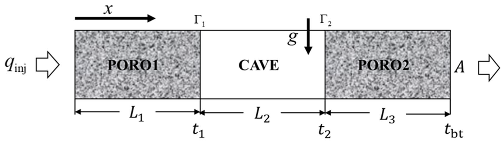
As illustrated in Figure 1, the composite model consists of three sequential segments: a porous medium (PORO1) of length L₁, a cave (CAVE) of length L₂, and a second porous medium (PORO2) of length L₃. The system is initially saturated with oil and has a constant cross-sectional area A. Water is injected at the left inlet with a constant flow rate q_inj. The arrival times of the water front at interfaces Γ₁ and Γ₂ are denoted as t₁ and t₂, respectively, while the breakthrough time at the model outlet is denoted as t_bt.

In the porous media regions, fluid flow is governed by the mass conservation equation and Darcy’s law,

$${\displaystyle \frac{\partial \left(\begin{array}{c}{\rho }_i{S}_i\varphi \end{array}\right)}{\partial t}}+\nabla \cdot \left(\begin{array}{c}{\rho }_i{\mathit{v}}_i\end{array}\right)=0, i=\mathrm{w},\mathrm{o} ,$$

(1)

$${\mathit{v}}_i=-{\displaystyle \frac{k{k}_{ri}}{{\mu }_i}}\nabla P_i, i=\mathrm{w},\mathrm{o},$$

(2)

where the subscript i denotes the fluid phase (w for water, o for oil); ρ_i, S_i and μ_i represent the density, saturation, and viscosity of the phase i, respectively, and the phase saturations satisfy

$$S_{\mathrm{w}}+S_{\mathrm{w}}=1;$$

(3)

where k_ri is the relative permeability; ϕ is the porosity; P_i is the phase pressure; k is the absolute permeability; v_i is the Darcy velocity vector and in the following one-dimensional derivation, and its axial component is denoted by u_i:

$${\mathit{v}}_i=\left(u_i,0,0\right).$$

(4)

For the cave region, the water volume fraction α on any cross-section is defined as the ratio of the water phase area to the total cross-sectional area. Under the incompressible-flow assumption, the water-phase conservation equation and the averaged momentum balance in the cave are written as follows:

$${\displaystyle \frac{\partial \left({\rho }_{\mathrm{w}}\alpha A\right)}{\partial t}}+\nabla \cdot \left(\mathit{v}{\rho }_{\mathrm{w}}\alpha A\right)=0,$$

(5)

$$\rho \left({\displaystyle \frac{\partial \mathit{v}}{\partial t}}+\mathit{v}\cdot \nabla \mathit{v}\right)=-\nabla p+\nabla \cdot \mu \left(\nabla \mathit{v}+\nabla {\mathit{v}}^{\mathrm{T}}\right),$$

(6)

where v denotes the cross-sectionally averaged fluid velocity within the cave; ρ and μ represent the average density and viscosity of the fluid, respectively. Based on the above definition of the water volume fraction α, the averaged density and viscosity in the cave are closed as

$$\rho =\alpha {\rho }_{\mathrm{w}}+\left(1 - \alpha \right){\rho }_{\mathrm{o}},$$

$$\mu =\alpha {\mu }_{\mathrm{w}}+\left(1 - \alpha \right){\mu }_{\mathrm{o}},$$

where ρ_w, ρ_o, μ_w, and μ_o are the densities and viscosities of the water and oil phases, respectively.

2.2. Derivation of Fractional Flow and Buckley–Leverett Equation

Based on the condition of constant cross-sectional area, the oil flow rate q_o and water flow rate q_w can be expressed as

$$q_i=A{u}_i, i = \mathrm{w}, \mathrm{o}.$$

(7)

$$q_{\mathrm{t}}=q_{\mathrm{w}}+q_{\mathrm{o}}.$$

(8)

where q_t is the total flow rate. Substituting Equation (7) into Equation (2) yields the flow rate expressions for phase i,

$$q_i=-Ak{\displaystyle \frac{k_{ri}}{{\mu }_i}}{\displaystyle \frac{\partial P}{\partial x}}, i = \mathrm{w}, \mathrm{o},$$

(9)

where $P$ denotes the common pressure gradient used in the present formulation under the assumption that capillary-pressure gradients are neglected.

Defining the fractional flow f_i as the ratio of the volumetric flow rate of phase i to the total flow rate, the water fractional flow f_w and oil fractional flow f_o are given by

$$f_i={\displaystyle \frac{q_i}{q_{\mathrm{t}}}}, i = \mathrm{w}, \mathrm{o},$$

(10)

$$f_{\mathrm{o}}+f_{\mathrm{w}}=1.$$

(11)

Substituting Equation (10) into Equation (9) and using the constraint in Equation (11), the two resulting phase-flow equations are solved simultaneously to obtain the water fractional flow function,

$$f_{\mathrm{w}}={\displaystyle \frac{1}{1 + \frac{k_{\mathrm{ro}}}{k_{\mathrm{rw}}}\cdot \frac{{\mu }_{\mathrm{w}}}{{\mu }_{\mathrm{o}}}}}.$$

(12)

Based on the incompressibility of the fluids, the mass conservation Equation (1) simplifies to

$$-{\displaystyle \frac{\partial u_i}{\partial x}} = {\displaystyle \frac{\partial }{\partial t}}\left(S_i\varphi \right), i = \mathrm{w}, \mathrm{o}.$$

(13)

Substituting Equation (7) into Equation (13) gives

$$-{\displaystyle \frac{\partial q_i}{\partial x}}=A\varphi {\displaystyle \frac{\partial S_i}{\partial t}}, i = \mathrm{w}, \mathrm{o}.$$

(14)

Further substituting Equation (10) into Equation (14) yields

$$-{\displaystyle \frac{\partial f_i}{\partial x}}={\displaystyle \frac{A\varphi }{q_{\mathrm{t}}}}{\displaystyle \frac{\partial S_i}{\partial t}}, i = \mathrm{w}, \mathrm{o}.$$

(15)

Taking the water-phase form of Equation (15), the characteristic form can be derived by considering the total differential of S_w, as follows

$$\mathrm{d}{S}_{\mathrm{w}}={\left.{\displaystyle \frac{\partial S_{\mathrm{w}}}{\partial x}}\right|}_t\mathrm{d}x+{\left.{\displaystyle \frac{\partial S_{\mathrm{w}}}{\partial t}}\right|}_x\mathrm{d}t.$$

(16)

By tracking the movement of a specific iso-saturation plane,

$${\left.{\displaystyle \frac{\partial S_{\mathrm{w}}}{\partial t}}\right|}_x=-{\left.{\displaystyle \frac{\partial S_{\mathrm{w}}}{\partial x}}\right|}_t\cdot {\left.{\displaystyle \frac{\mathrm{d}x}{\mathrm{d}t}}\right|}_{S_{\mathrm{w}}}.$$

(17)

Substituting Equation (17) into Equation (15) yields

$$-{\left.{\displaystyle \frac{\partial f_{\mathrm{w}}}{\partial S_{\mathrm{w}}}}\right|}_t\cdot {\left.{\displaystyle \frac{\partial S_{\mathrm{w}}}{\partial x}}\right|}_t=-{\displaystyle \frac{A\varphi }{q_{\mathrm{t}}}}{\left.{\displaystyle \frac{\partial S_{\mathrm{w}}}{\partial x}}\right|}_t\cdot {\left.{\displaystyle \frac{\mathrm{d}x}{\mathrm{d}t}}\right|}_{S_{\mathrm{w}}}.$$

(18)

Simplifying this result leads to the equation for the saturation advancement velocity

$${\left.{\displaystyle \frac{\mathrm{d}x}{\mathrm{d}t}}\right|}_{S_{\mathrm{w}}}={\displaystyle \frac{q_{\mathrm{t}}}{A\varphi }}\cdot {\left.{\displaystyle \frac{\partial f_{\mathrm{w}}}{\partial S_{\mathrm{w}}}}\right|}_t.$$

(19)

Upon integration, the analytical Buckley–Leverett solution for water flooding in a one-dimensional linear porous domain is obtained as

$$x\left(S_{\mathrm{w}}\right)={\displaystyle \frac{1}{A\varphi }}\cdot {\displaystyle \frac{\mathrm{d}{f}_{\mathrm{w}}}{\mathrm{d}{S}_{\mathrm{w}}}}\cdot {\displaystyle {\int }_0^t{q}_{\mathrm{t}}}\left(\tau \right)\mathrm{d}\tau .$$

(20)

2.3. Proof of Constant Total Flux Across All Domains

For later use in the piecewise analytical solution, this subsection establishes that the total volumetric flow rate remains equal to the prescribed injection rate throughout the one-dimensional PCP system.

2.3.1. Porous-Medium Region 1 (PORO1)

Adding the water- and oil-phase forms of Equation (14) gives

$$-{\displaystyle \frac{\partial }{\partial x}}\left(q_{\mathrm{o}}+q_{\mathrm{w}}\right)=A\varphi {\displaystyle \frac{\partial }{\partial t}}\left(S_{\mathrm{o}}+S_{\mathrm{w}}\right).$$

(21)

Using the saturation constraint in Equation (3), the accumulation term on the right-hand side vanishes:

$${\displaystyle \frac{\partial q_{\mathrm{t}}}{\partial x}}=0, q_{\mathrm{t}} = q_{\mathrm{o}} + q_{\mathrm{w}}.$$

(22)

Here, q_t is the total volumetric flow rate. Thus, q_t is spatially constant in PORO1, with the prescribed inlet flow rate

$$q_{\mathrm{t}}\left(x,t\right)=q_{\mathrm{inj}}, 0\le x\le L_1.$$

(23)

2.3.2. Cave Region (CAVE)

To formulate the flux-continuity conditions at the two internal interfaces, the variables on the two sides of each interface must be distinguished. This is necessary because the transported state may be remapped across an interface; for example, water saturation in a porous domain is mapped to water volume fraction in the cave. Therefore, interface limits are introduced as

$$F\left({{\Gamma }_m}^{-},t\right)=\underset{x\to x_m^{-}}{\mathit{lim}}\left(F\left(x,t\right)\right), F\left({{\Gamma }_m}^{+},t\right)=\underset{x\to x_m^{+}}{\mathit{lim}}\left(F\left(x,t\right)\right), m=1,2.$$

Here, x₁ = L₁, x₂ = L₁ + L₂, and F denotes a generic flow variable such as phase flux, saturation, or water volume fraction. For the present left-to-right displacement, Γ_m⁻ and Γ_m⁺ denote the upstream and downstream limits at interface Γ_m, respectively. This notation is used to specify flux continuity and state mapping, and does not imply saturation continuity across the interface.

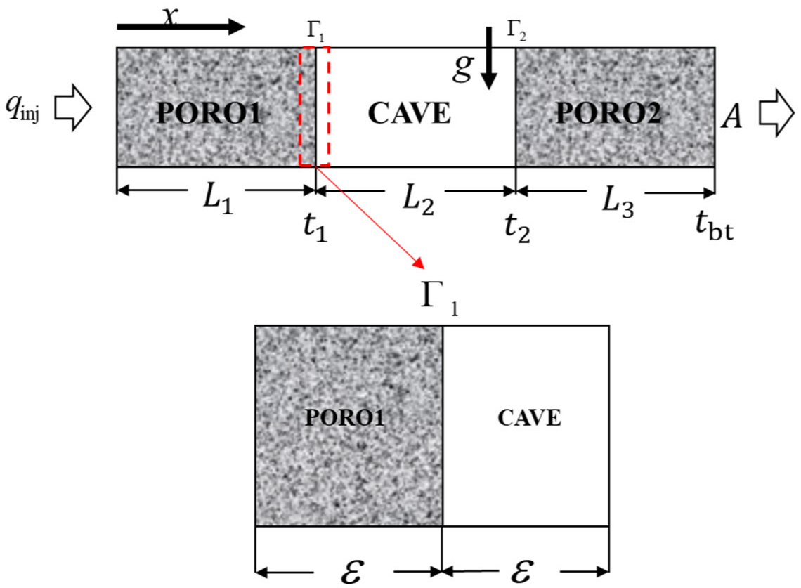
Applying phase-wise mass conservation to an infinitesimal control volume enclosing Γ₁, with no interfacial storage (as shown in Figure 2), gives

$$q_i{|}_{{L_1}^{-}}=q_i{|}_{{L_1}^{+}}, i = \mathrm{w}, \mathrm{o},$$

(24)

Therefore, the total flow rate entering the cave equals that leaving PORO1,

$$q_{\mathrm{t}}{|}_{{L_1}^{-}}=q\mathrm{t}{|}_{{L_1}^{+}}=q_{\mathrm{inj}}.$$

(25)

Within the cavity, the incompressible-flow continuity gives

$$\nabla \cdot \mathit{v}=0.$$

(26)

Since the cavity side walls are impermeable and flow occurs only through the inlet and outlet cross-sections, the total flow rate remains constant along the cave:

$$q_{\mathrm{t}}\left(x,t\right)=q_{\mathrm{inj}}, L_1\le x\le L_1 + L_2.$$

(27)

2.3.3. Porous-Medium Region 2 (PORO2)

The same no-storage interface condition at Γ₂ gives continuity of the total flow rate between the cave and PORO2. Hence,

$$q_{\mathrm{t}}\left(x,t\right)=q_{\mathrm{inj}}, L_1 + L_2 < x \le L_1 + L_2+L_3.$$

(28)

Combining the three segments, the total volumetric flow rate throughout the PCP system is

$$q_{\mathrm{t}}\left(x,t\right)=q_{\mathrm{inj}}, 0 < x \le L_1 + L_2 + L_3.$$

(29)

Because the cross-sectional area A is constant, the corresponding total axial superficial velocity is denoted by u_t:

$$u={\displaystyle \frac{q_{\mathrm{inj}}}{A}}={\displaystyle \frac{q_{\mathrm{t}}}{A}},$$

(30)

2.4. Analytical Solution of the Porous–Cavernous–Porous System

Based on the governing equations established above, the PCP solution is constructed segment by segment. For each segment, the corresponding saturation or water volume fraction solution is first obtained, and the critical time nodes associated with front propagation across the internal interfaces are then determined. In this way, the complete analytical description of the displacement process in the PCP system can be constructed by matching the solutions across the two interfaces Γ₁ and Γ₂.

2.4.1. PORO1: Buckley–Leverett Solution and Front Arrival at Γ₁

PORO1 serves as the starting segment of the composite system. Based on the assumption that downstream flow does not affect upstream flow, the saturation distribution follows the standard Buckley–Leverett solution

$$x(S_{\mathrm{w}})={\displaystyle \frac{1}{A\varphi }}\cdot {\displaystyle \frac{\mathrm{d}{f}_{\mathrm{w}}}{\mathrm{d}{S}_{\mathrm{w}}}}\cdot {\displaystyle {\int }_0^t{q}_{\mathrm{inj}}}\left(\tau \right)\mathrm{d}\tau , 0\le x\le L_1,$$

(31)

The leading shock front is represented by the shock-front water saturation S_wf,p1, where the subscript wf denotes the shock-front water state and p1 denotes PORO1. This saturation is determined from the Welge tangent condition for PORO1. Its arrival at the first interface Γ₁ is therefore obtained:

$$t_1={\displaystyle \frac{A{\varphi }_1{L}_1}{q_{\mathrm{inj}}\frac{\mathrm{d}{f}_{\mathrm{w}}}{\mathrm{d}{S}_{\mathrm{w}}}{|}_{S_{\mathrm{wf},\mathrm{p}1}}}},$$

(32)

where ϕ₁ is the porosity of the region PORO1.

2.4.2. CAVE: Water Volume Fraction Solution and Transit to Γ₂

After the leading shock front reaches Γ₁, the water-bearing flow from PORO1 enters the cave region. This subsection formulates how the incoming fractional flow signal is represented as a water volume fraction signal and transported within the cave under the cross-sectionally averaged plug-flow approximation.

Consistent with the one-dimensional velocity representation introduced in Equation (4), the cave velocity is reduced to its cross-sectionally averaged axial component u.

Taking the axial component of the cave momentum equation, Equation (6), under the velocity field gives

$$\rho \left({\displaystyle \frac{\partial u}{\partial t}}+u{\displaystyle \frac{\partial u}{\partial x}}\right)=-{\displaystyle \frac{\partial p}{\partial x}}+{\displaystyle \frac{\partial }{\partial x}}\left(2\mu {\displaystyle \frac{\partial u}{\partial x}}\right), L_1\le x\le L_1 + L_2.$$

(33)

According to Equation (30),

$${\displaystyle \frac{\partial u}{\partial t}}=0,{\displaystyle \frac{\partial u}{\partial x}}=0.$$

(34)

Since u is constant in both space and time, the axial acceleration and viscous-diffusion terms vanish. The idealized open-cave momentum equation therefore reduces to

$${\displaystyle \frac{\partial p}{\partial x}}=0, L_1\le x\le L_1 + L_2,$$

(35)

and this zero-pressure-gradient result is a consequence of the cross-sectionally averaged plug-flow idealization. It does not resolve wall shear, transverse recirculation, buoyancy segregation, or interfacial redistribution inside the cave.

Under the plug-flow approximation, the water flux across a cave cross-section is αq_t, whereas the water flux supplied from PORO1 is f_w,p1q_t. Flux continuity at Γ₁ therefore gives

$$\alpha =f_{\mathrm{w},\mathrm{p}1}\left(S_{\mathrm{w},{\mathrm{p}}_1}\right),$$

(36)

which maps a general saturation state in PORO1 into a water volume fraction signal in the cave. In particular, the PORO1 shock-front water saturation gives the cave front signal,

$${\alpha }_{\mathrm{f}}=f_{\mathrm{wf},\mathrm{p}1}\left(S_{\mathrm{wf},\mathrm{p}1}\right),$$

(37)

For the water phase in the cave, mass conservation from Equation (5) with constant density gives

$${\displaystyle \frac{\partial \alpha }{\partial t}}+\nabla \cdot \left(\mathit{v}\alpha \right)=0.$$

(38)

Combined with Equation (26), Equation (38) reduces to

$${\displaystyle \frac{\partial \alpha }{\partial t}}+\mathit{v}\cdot \nabla \alpha =0,$$

(39)

which signifies that the material derivative of the water volume fraction α is zero,

$${\displaystyle \frac{\mathrm{D}\alpha }{\mathrm{D}t}}=0.$$

(40)

Thus, the water volume fraction signal is conserved along a plug-flow trajectory. Equivalently, the signal at position x and time t is the inlet signal at Γ₁ evaluated at an earlier time,

$$t^{*}=t-{\displaystyle \frac{x-L_1}{u}}.$$

(41)

Therefore,

$$\alpha \left(x,t\right)=f_{\mathrm{w},\mathrm{p}1}(S_{\mathrm{w}}(L_1,t-{\displaystyle \frac{x-L_1}{u}}\left)\right), L_1\le x\le L_1 + L_2.$$

(42)

The corresponding transit time t_α through the cave is

$$t_{\alpha }={\displaystyle \frac{L_2}{u}}={\displaystyle \frac{A{L}_2}{q_{\mathrm{inj}}}}.$$

(43)

Therefore, the total time t₂ required for the water front to reach the interface Γ₂ is

$$t_2=t_1 + t_{\alpha }={\displaystyle \frac{A{\varphi }_1{L}_1}{q_{\mathrm{inj}}\frac{\mathrm{d}{f}_{\mathrm{w}}}{\mathrm{d}{S}_{\mathrm{w}}}{|}_{S\mathrm{wf},\mathrm{p}1}|}}+{\displaystyle \frac{A{L}_2}{q_{\mathrm{inj}}}}.$$

(44)

Under the present one-dimensional plug-flow approximation, the cave acts as a pure transmission-delay segment, so the front signal reaching Γ₂ is simply the front signal arriving at Γ₁ shifted by the cave transit time t_α. Thus, no additional Buckley–Leverett shock structure is generated inside the cave.

2.4.3. PORO2: Delayed-Entry Solution and Front-Position Determination

After the cave front signal reaches Γ₂, the transmitted water volume fraction signal enters PORO2 and is remapped into a water-saturation state according to the fractional flow relation of PORO2. The downstream porous domain still follows the Buckley–Leverett equation, but its solution starts from Γ₂ with a saturation-dependent entry time.

For a general saturation state S_w,p2, the characteristic position in PORO2 is measured from the second interface Γ₂,

$$x-L_1-L_2={\displaystyle \frac{q_{\mathrm{inj}}}{A{\varphi }_2}}{\displaystyle \frac{\mathrm{d}{f}_{\mathrm{w},\mathrm{p}2}}{\mathrm{d}{S}_{\mathrm{w}}}}\left(t-t_s\right),$$

(45)

where t_s represents the time at which this specific saturation value enters PORO2 at the interface Γ₂; ϕ₂ is the porosity of the region PORO2.

At Γ₂, the water-fraction signal entering PORO2 equals the PORO1 fractional flow signal delayed by the cave transit time t_α. Hence, for a general downstream saturation state entering PORO2 at time t_s,

$$f_{\mathrm{w},\mathrm{p}2}\left({S_{\mathrm{w},\mathrm{p}2}}^{+}\left(t_s\right)\right)=f_{\mathrm{w},\mathrm{p}1}\left({S_{\mathrm{w},\mathrm{p}1}}^{-}(t_s-t_{\alpha })\right),$$

(46)

because different saturation states are transmitted from the cave at different times, t_s is saturation-dependent. The entry time of S_w,p2 is then determined by comparing this upstream-equivalent saturation with the PORO1 shock-front water saturation.

• If the corresponding upstream saturation is greater than the PORO1 shock-front water saturation, the associated characteristic state enters PORO2 continuously,

$$t_s=t_{\alpha }+{\displaystyle \frac{A{\varphi }_1{L}_1}{q_{\mathrm{inj}}\frac{\mathrm{d}{f}_{\mathrm{w}}}{\mathrm{d}{S}_{\mathrm{w}}}{|}_{{S_{\mathrm{w},\mathrm{p}1}}^{-}}}}, {S_{\mathrm{w},\mathrm{p}1}}^{-}>S_{\mathrm{wf},\mathrm{p}1};$$

(47)

• If the corresponding upstream saturation is less than or equal to the PORO1 shock-front water saturation, the entry time is controlled by the arrival of the cave front signal,

$$t_s=t_{\alpha }+t_1, {S_{\mathrm{w},\mathrm{p}1}}^{-}\le S_{\mathrm{wf},\mathrm{p}1}.$$

(48)

The downstream front position is determined from the global water-balance closure. Let W be the cumulative injected water volume, and let W_p1, W_c, and W_p2 denote the water volumes retained in PORO1, the cave, and PORO2, respectively. Then,

$$W_{\mathrm{p}2}=W-W_{\mathrm{p}1}-W_c,$$

(49)

where

$$W=q_{\mathit{inj}}t,$$

(50)

$$W_{\mathrm{p}1}=A{\varphi }_1{\displaystyle {\int }_0^{L_1}\left(S_{\mathrm{w},\mathrm{p}1}\left(x\right)-S_{\mathrm{wc},\mathrm{p}1}\right)\mathrm{d}x},$$

(51)

$$W_c=A{\displaystyle {\int }_{L_1}^{L_1+L_2}\alpha \left(x\right)\mathrm{d}x}.$$

(52)

$$W_{\mathrm{p}2}=A{\varphi }_2{\displaystyle {\int }_{L_1+L_2}^{x\mathrm{f},\mathrm{p}2}\left(S_{\mathrm{w},\mathrm{p}2}(x,t)-S_{\mathrm{wc},\mathrm{p}2}\right)\mathrm{d}x}$$

(53)

Substituting the above expressions into the water-balance closure gives

$$A{\varphi }_2{\displaystyle {\int }_{L_1+L_2}^{x\mathrm{f},\mathrm{p}2}\left(S_{\mathrm{w},\mathrm{p}2}(x,t)-S_{\mathrm{wc},\mathrm{p}2}\right)\mathrm{d}x}=q_{\mathrm{inj}}t-A{\varphi }_1{\displaystyle {\int }_0^{L_1}\left(S_{\mathrm{w},\mathrm{p}1}\left(x\right)-S_{\mathrm{wc},\mathrm{p}1}\right)\mathrm{d}x}-A{\displaystyle {\int }_{L_1}^{L_1+L_2}\alpha \left(x\right)\mathrm{d}x}.$$

(54)

Solving this equation gives the downstream front position x_f,p2. The corresponding front water saturation $S_{\mathrm{wf},\mathrm{p}2}$ is determined by the interfacial fractional flow mapping in Equation (46).

2.5. Computational Realization of the Piecewise Semi-Analytical Solution

The piecewise semi-analytical solution is implemented in the same sequence as the theoretical construction: PORO1, CAVE, and PORO2. In PORO1, the Buckley–Leverett/Welge solution gives the upstream shock-front water saturation and its arrival time at Γ₁. In the cave, the incoming fractional flow signal is transformed into a water volume fraction signal and shifted by the cave transit time. In PORO2, the transmitted signal is remapped through the downstream fractional flow relation, and the front position is determined from the global water-balance closure. Thus, explicit analytical relations are used for PORO1 and CAVE, whereas a numerical search is required only for the implicit downstream closure in PORO2. The detailed computational procedure is summarized in Algorithm 1.

Algorithm 1. Computational realization of the piecewise semi-analytical PCP solution.
Input: model parameters of PCP system; injection rate qinj; evaluation time t
1:	generate tabulated curves {Sw, krw, kro, fw, dfw/dSw} for PORO1 and PORO2
2:	determine the upstream shock-front water saturation Swf,p1
3:	compute the arrival time t1 at Γ1 and the delayed arrival time t2 at Γ2
4:	if (t < t1) then
5:	construct PORO1 profile
6:	else if (t1 < t ≤ t2) then
7:	construct PORO1 and CAVE profiles
8:	else
9:	construct PORO1 and CAVE profiles, and compute Wp1 and Wc
10:	set the target downstream water volume Wp2 = W − Wp1 − Wc
11:	for (candidate Sw,p2 in PORO2) do
12:	interpolate ts and x
13:	update the accumulated downstream water volume by profile integration
14:	stop when the accumulated volume reaches Wp2
15:	end for
16:	identify the downstream front position in PORO2
17:	end if
Output: front position; saturation/volume-fraction profiles; recovery indicators.

For PORO2, the downstream solution is not fully explicit because the entry time $t_{\mathrm{s}}$ depends on the transmitted saturation state and the front position must also satisfy the global water-balance closure. Therefore, the downstream front is obtained by a one-dimensional numerical search over the tabulated saturation states. For each candidate S_w,p2 the corresponding upstream-equivalent state, delayed entry time, and characteristic position are evaluated. The PORO2 water-content profile is then integrated until the accumulated water volume matches W_p2. The search is terminated when the relative water-balance residual satisfies

$${\epsilon }_{\mathrm{w}}=\left|{\displaystyle \frac{w_{\mathrm{cal}}-w_{\mathrm{p2}}}{w_{\mathrm{p2}}}}\right|\le {\epsilon }_{\mathrm{tol}}.$$

(55)

Because the present PCP solution is obtained in a piecewise semi-analytical manner, its implementation is checked from three complementary consistency requirements. First, within each segment, the adopted analytical relations must remain consistent with the corresponding governing equations: the PORO1 solution must recover the standard Buckley–Leverett/Welge construction, while the open-cave solution must satisfy the delayed-translation form implied by the cross-sectionally averaged cavity transport equation under the plug-flow assumption. Second, at the two internal interfaces, the transmitted front states must satisfy the prescribed flux-continuity and state-remapping relations, so that the signal passed from PORO1 to CAVE and from CAVE to PORO2 remains dynamically consistent with the piecewise formulation. Third, for the full PCP system, the downstream front determination must satisfy the global water-balance closure exactly, i.e., at any evaluation time, the total injected water volume equals the sum of the water retained in PORO1, CAVE, and PORO2. These checks do not constitute an experimental validation; rather, they provide an internal verification of the present implementation and of its consistency with established Buckley–Leverett-type theory for homogeneous, composite, and non-Darcy displacement problems.

3. Results

To ensure consistent comparisons across regions, we first characterize the relative permeability in the two porous segments and then analyze the cross-interface mapping and spatiotemporal evolution of the displacement front in the composite pore-cave-pore system. The relative permeability is described using the Brooks–Corey model [21,22].

$$k_{\mathrm{rw}}=k_{\mathrm{rw},\max }{\left({\displaystyle \frac{S_{\mathrm{w}}-S_{\mathrm{wc}}}{1-S_{\mathrm{wc}}-S_{\mathrm{or}}}}\right)}^{n_{\mathrm{w}}},$$

(56)

$$k_{\mathrm{ro}}=k_{\mathrm{ro},\max }{\left({\displaystyle \frac{1-S_{\mathrm{w}}-S_{\mathrm{or}}}{1-S_{\mathrm{wc}}-S_{\mathrm{or}}}}\right)}^{n_{\mathrm{o}}}.$$

(57)

3.1. Stage-Wise Front Propagation Across the PCP System

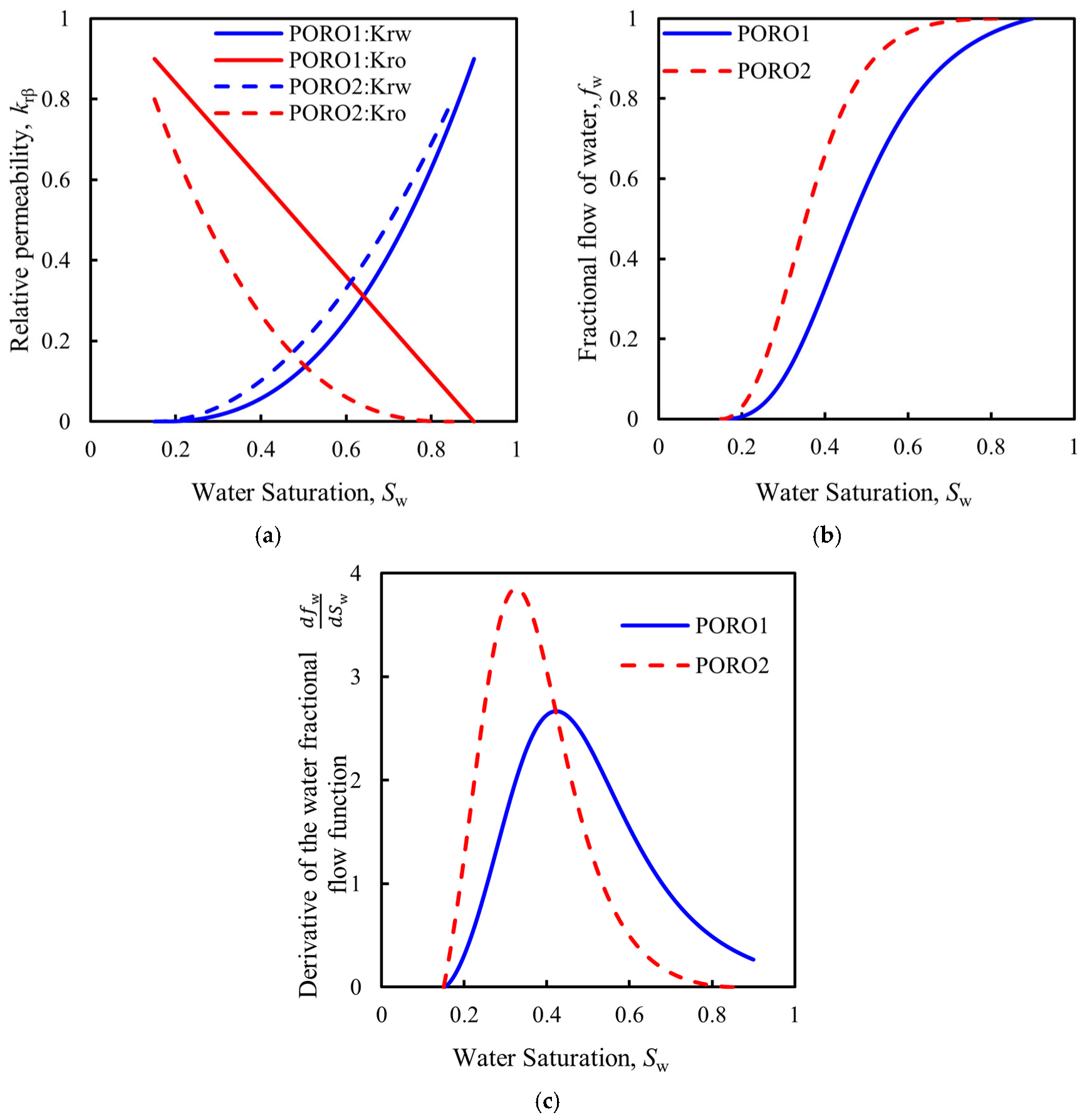
A cave length of 10 m is prescribed, and the base physical parameters for the porous media regions are listed in

Table 1. Base physical parameters used in the reference PCP case.

Parameters	PORO1	PORO2	Unit
porosity of domains, ϕ	0.25	0.25	[-]
permeability, k	9.869 × 10−13	9.869 × 10−13	[m2]
length of domains, L	60	60	[m]
cross-sectional area, A	1.00	1.00	[m2]
injection rate, qinj	1.0 × 10−4	-	[m3/s]
water phase viscosity, μw	1.0	1.0	[mPa∙s]
oil phase viscosity, μo	5.0	5.0	[mPa∙s]
initial water phase saturation, Swc	0.15	0.15	[-]
residual oil saturation, Sor	0.10	0.15	[-]
relative permeability parameters, krw,max	0.90	0.80	[-]
relative permeability parameters, kro,max	0.90	0.80	[-]
relative permeability parameters, nw	2.50	2.00	[-]
relative permeability parameters, no	1.00	1.50	[-]
density of wetting fluid, ρw	1000	1000	[kg/m3]
density of non-wetting fluid, ρo	800	800	[kg/m3]

. The values in Table 1 are selected as representative idealized parameters for illustrating stage-wise front propagation in the reference PCP case, rather than as a field-calibrated parameter set for a specific fractured-vuggy reservoir. Based on these parameters, the relative permeability, fractional flow curves, and their derivatives for PORO1 and PORO2 are calculated (see Figure 3).

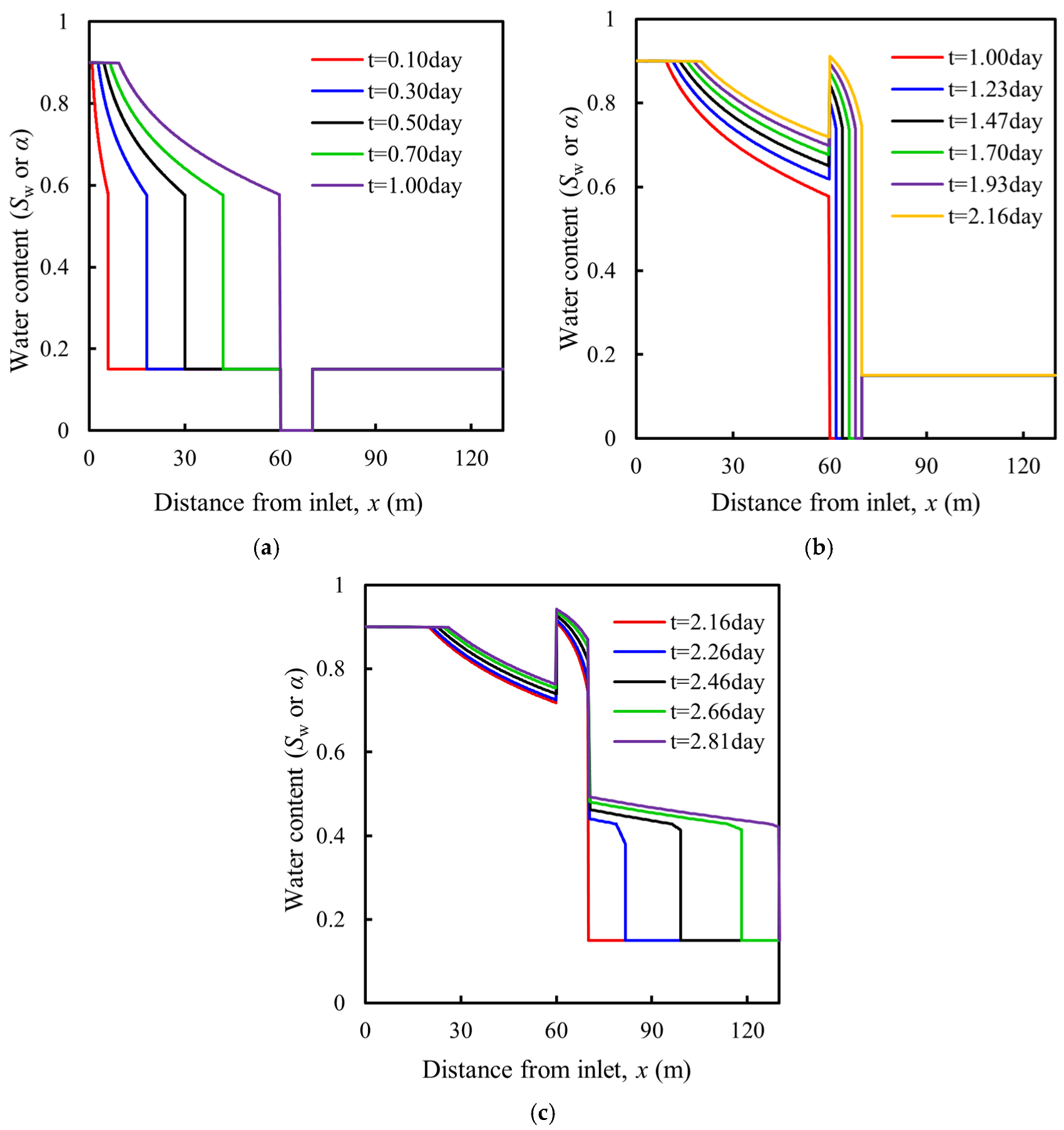
Figure 4 illustrates the three evolutionary stages of the water-oil displacement process within the porous–cavernous–porous composite system, characterized by distinct spatiotemporal behaviors:

Stage 1 (0 < t ≤ 1.00 day): the water front advances steadily within PORO1 (Figure 4a). The saturation profile exhibits typical Buckley–Leverett characteristics, where a rarefaction wave originates from the inlet and is terminated by a shock front. During this stage, the cave and PORO2 remain at their initial oil-saturated states. At 1.00 day, the shock front precisely reaches the first interface Γ₁.

Stage 2 (1.00 < t ≤ 2.16 day): the water volume fraction front signal is transmitted through the cave region (Figure 4b). The exit saturation S_w,p1 from PORO1 is converted into a higher water volume fraction at the interface Γ₁, which remains constant as it is transmitted downstream. Due to the significantly higher storage capacity of the cave compared to the porous matrix, the cave front signal takes over one day to traverse only 10 m, resulting in a marked deceleration of the frontal advancement.

Stage 3 (t > 2.16 day): the transmitted cave front signal enters PORO2 and is remapped into a downstream saturation state (Figure 4c). As the two-phase fluid crosses the second interface Γ₂, PORO2 re-maps the volume fraction into a new inlet water saturation S_w,p2 based on its specific constitutive relationship, giving rise to a new shock-rarefaction wave structure.

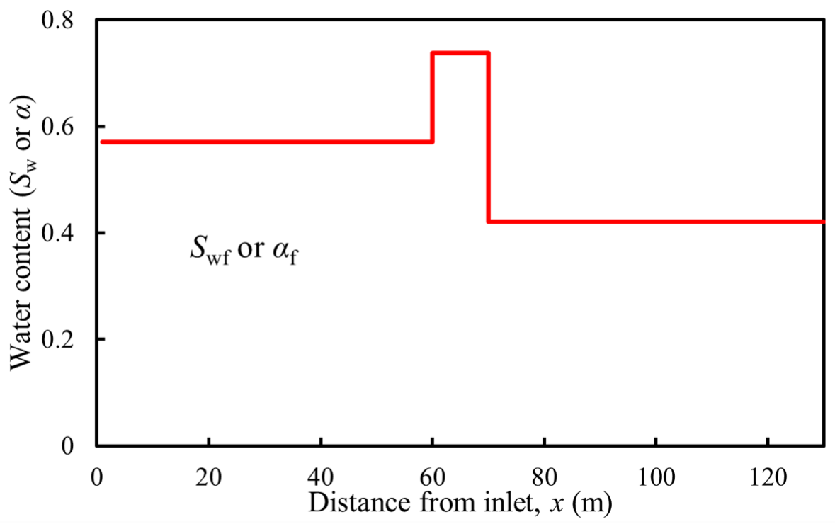
Figure 5 illustrates the front-state remapping mechanism obtained from the piecewise solution. In PORO1, the shock-front water saturation S_wf,p1 is determined by the Welge tangent condition and serves as the upstream reference front state. After reaching Γ₁, this state is not transmitted downstream as saturation itself; instead, it is converted into the cave front signal α_f through the fractional flow relation. Under the present plug-flow approximation, the cave does not generate a new Buckley–Leverett shock structure, but transmits this front signal with a finite time delay. At Γ₂, the transmitted signal is remapped through the fractional flow relation of PORO2 to determine the downstream shock-front water saturation S_wf,p2. Therefore, the downstream front state is a reconstructed state controlled by interfacial transmission and the constitutive properties of PORO2, rather than a direct continuation of the upstream saturation profile.

3.2. Effect of Cave Length on Front Delay and Breakthrough Recovery

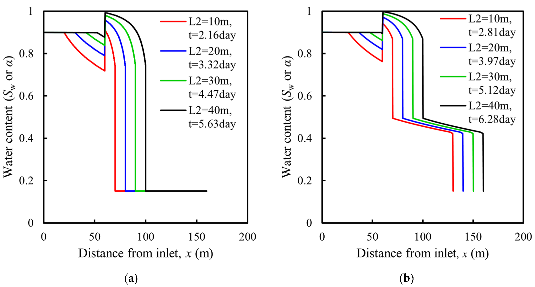
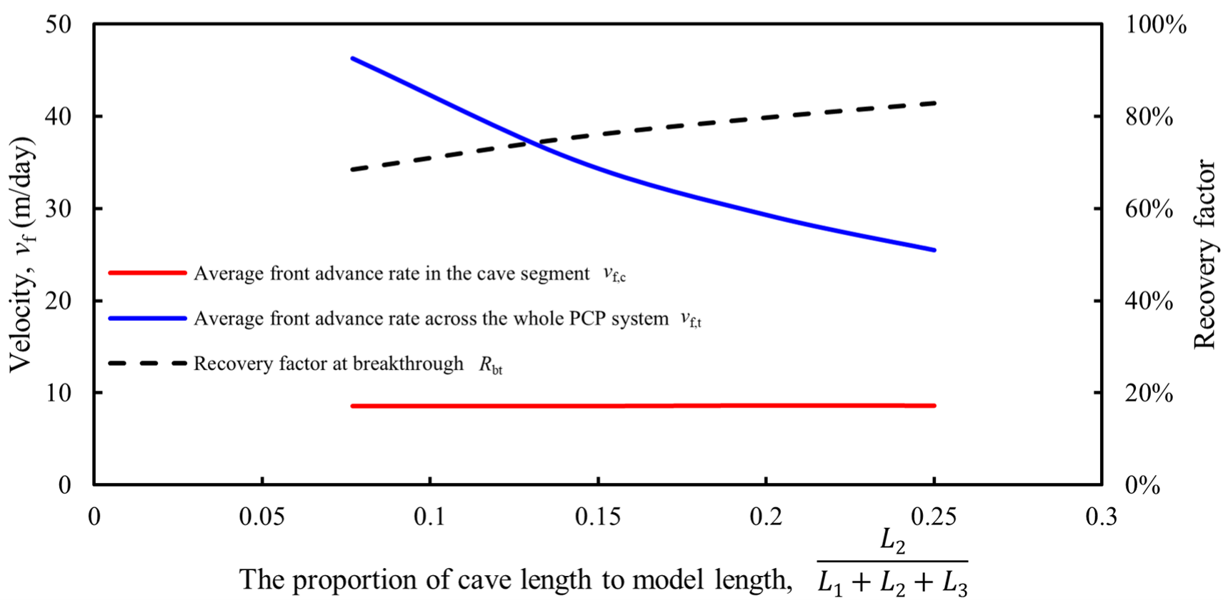
Under constant boundary conditions, the impact of cave lengths (10, 20, 30, and 40 m) was analyzed, with results shown in Figure 6 and Figure 7. This length range was selected to cover the meter- to tens-of-meters scale of cave-like storage spaces reported in fractured-vuggy carbonate reservoirs; for example, field-based studies have reported that many karst caves are larger than 5 m and commonly within 20 m, whereas other fractured-vuggy systems or vuggy geobodies may extend to several tens of meters [23,24,25]. To quantify the effect of cave length on front propagation, two average front advance rates are introduced: v_f,t for the whole PCP system and v_f,c for the cave segment,

$$v_{\mathrm{f},\mathrm{t}}={\displaystyle \frac{L_1+L_2+L_3}{t_{\mathrm{bt}}}},$$

(58)

$$v_{\mathrm{f},\mathrm{c}}={\displaystyle \frac{L_2}{t_{\alpha }}}.$$

(59)

Here, v_f,c is independent of cave length under the present assumptions. However, as the proportion of the cave length relative to the total model length increases, the system-wide average frontal velocity v_f,t gradually decreases. This indicates that the effect of cave length is expressed mainly through increased storage volume and delayed breakthrough, rather than through a change in the local plug-flow velocity inside the cave.

Furthermore, the recovery factor at breakthrough R_bt is used here to characterize the displacement efficiency at the critical moment when the water front reaches the outlet. As the cave-length ratio increases from 0.077 to 0.250, R_bt increases from 0.69 to 0.83. Under the present parameter setting, this trend mainly reflects the increased storage capacity and delayed front propagation caused by a longer cave, rather than direct improvement of microscopic sweep efficiency in the porous matrix.

3.3. Effect of Forchheimer Non-Darcy Flow in Porous Domains on PCP Displacement Behavior

In the near-well region, where flow velocities can be high, fluid motion in porous media may deviate from the Darcy regime. To examine how non-Darcy resistance in the porous domains affects the response of the PCP system, the two-phase oil–water Forchheimer formulation is adopted following Wu [26]:

$$-{\displaystyle \frac{\partial P}{\partial x}}={\displaystyle \frac{{\mu }_i}{k{k}_{ri}}}{u}_i+{\rho }_i{\beta }_i{u}_i^2, i=\mathrm{w},\mathrm{o},$$

(60)

where β_i denotes non-Darcy flow coefficient, an intrinsic property of porous media [m⁻¹]. More generally, the non-Darcy coefficient is not a universal constant; its evaluation depends on the porous-medium structure and on the correlation adopted for its estimation [27,28]. In the present study, its phase-wise evaluation follows Wu [26],

$${\beta }_i={\displaystyle \frac{C_i}{{\left(k{k}_{ri}\right)}^{5/4}{\left[\varphi (S_i-S_{ir})\right]}^{3/4}}}, i=\mathrm{w},\mathrm{o},$$

(61)

where C_i is a non-Darcy flow constant with a unit of [m^3/2]. Because only the momentum relation is modified from Darcy to Forchheimer while the continuity equation remains unchanged, the one-dimensional Buckley–Leverett solution under non-Darcy flow differs primarily through the water fractional flow function. Under the stated assumptions, we therefore derive the modified fractional flow relation below. Equating the water- and oil-phase forms of Equation (60) eliminates the common pressure gradient and gives

$${\displaystyle \frac{{\mu }_{\mathrm{w}}}{k{k}_{\mathrm{rw}}}}{u}_{\mathrm{w}}+{\rho }_{\mathrm{w}}{\beta }_{\mathrm{w}}{u_{\mathrm{w}}}^2={\displaystyle \frac{{\mu }_{\mathrm{o}}}{k{k}_{\mathrm{ro}}}}{u}_{\mathrm{o}}+{\rho }_{\mathrm{o}}{\beta }_{\mathrm{o}}{u_{\mathrm{o}}}^2.$$

(62)

Using the total-velocity relation

$$u_{\mathrm{t}}=u_{\mathrm{w}}+u_{\mathrm{o}},$$

(63)

Equation (62) can be rearranged into a quadratic equation for u_w. For compactness, the following coefficients are introduced:

$$\begin{array}{c}a={\rho }_{\mathrm{w}}{\beta }_{\mathrm{w}}-{\rho }_{\mathrm{o}}{\beta }_{\mathrm{o}}\\ b={\displaystyle \frac{{\mu }_{\mathrm{w}}}{k{k}_{\mathrm{rw}}}}+{\displaystyle \frac{{\mu }_{\mathrm{o}}}{k{k}_{\mathrm{ro}}}}+2{\rho }_{\mathrm{o}}{\beta }_{\mathrm{o}}{u}_t\\ c=-{\displaystyle \frac{{\mu }_{\mathrm{o}}}{k{k}_{ro}}}{u}_t-{\rho }_{\mathrm{o}}{\beta }_{\mathrm{o}}{u}_t^2\end{array}.$$

(64)

The resulting quadratic equation is

$$a{u}_{\mathrm{w}}^2+b{u}_{\mathrm{w}}+c=0.$$

(65)

The physically admissible root is selected by enforcing

$$0<u_{\mathrm{w}}\le u_{\mathrm{t}},$$

(66)

that is, the water velocity must be nonnegative and cannot exceed the total velocity. The corresponding water fractional flow function is then obtained from

$$f_{\mathrm{w}}={\displaystyle \frac{u_{\mathrm{w}}}{u_t}}.$$

(67)

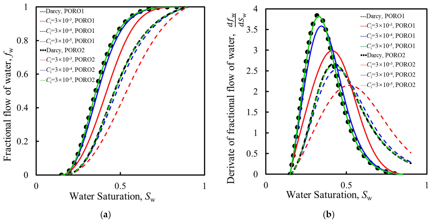
The two-phase fluid and porous-medium parameters remain those in Table 1, the cave length is fixed at 10 m, and the non-Darcy flow constant C_i is set to 3.0 × 10⁻³, 3.0 × 10⁻⁴, and 3.0 × 10⁻⁵ m^3/2. The resulting fractional flow functions and their derivatives under different non-Darcy constants are shown in Figure 8.

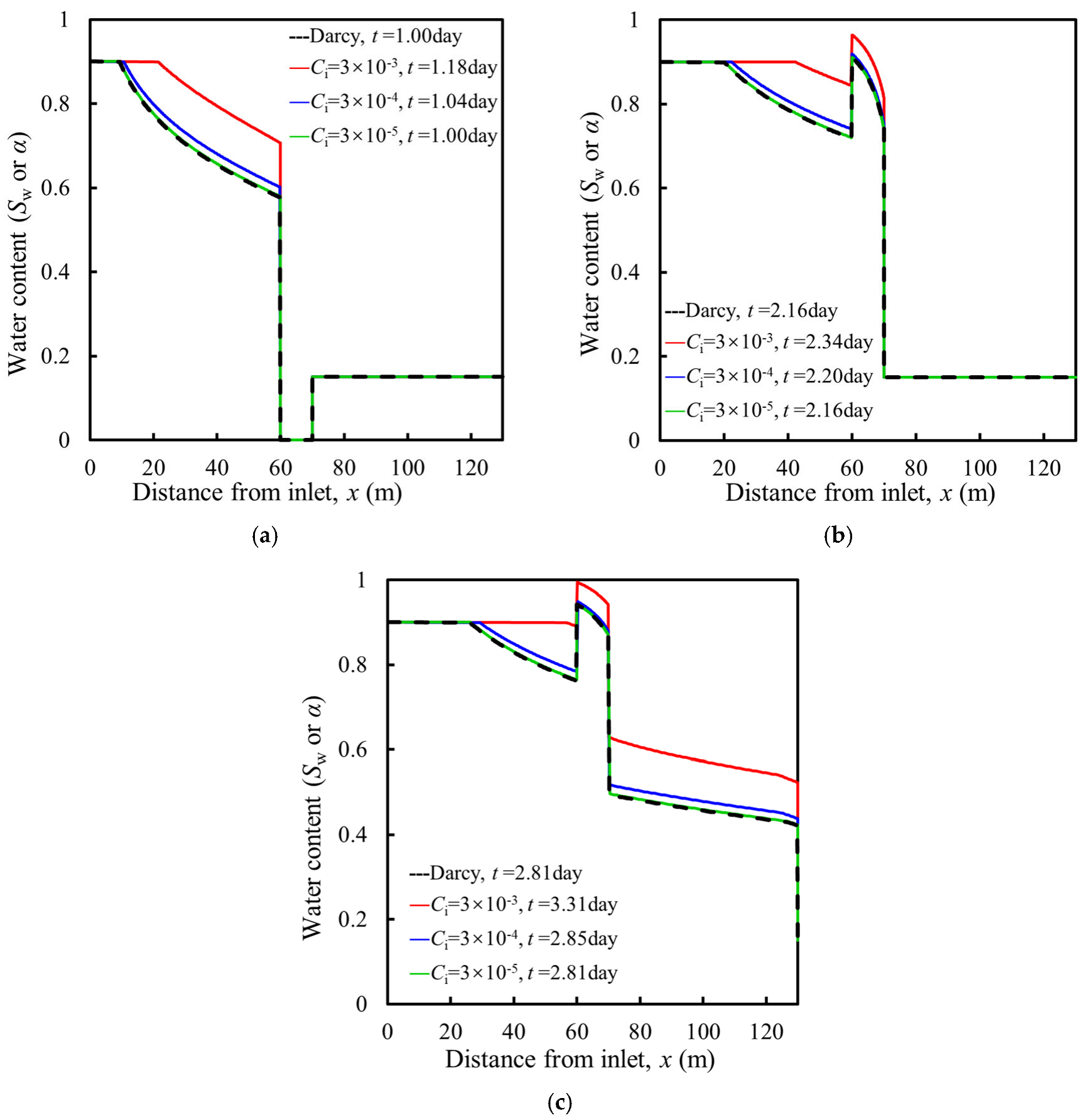
Figure 9 shows the PCP-system response when the porous domains are described by the Forchheimer formulation with different non-Darcy constants. As C_i increases, the front arrival at Γ₁, Γ₂, and the outlet is delayed successively; specifically, the outlet arrival time increases from 2.81 to 3.13 days over the tested range. Meanwhile, the front profiles become steeper than in the Darcy case, indicating that the Forchheimer correction modifies the fractional flow relation in the porous domains. In the present PCP framework, this effect is transmitted through the cave and ultimately appears as a delayed and restructured downstream displacement response.

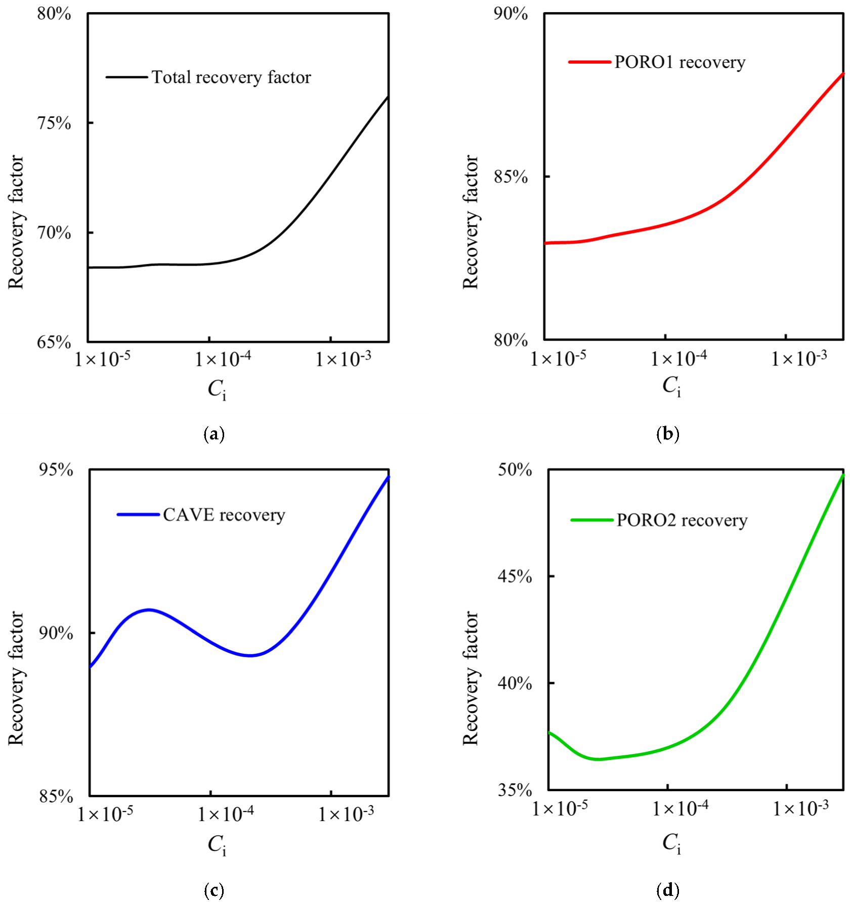
Figure 10 shows that the Forchheimer modification affects both the total recovery and the recovery contributions of the individual PCP segments. Over the tested range of C_i, the total recovery increases, while the recoveries of PORO1, CAVE, and PORO2 also vary accordingly. Under the present parameter setting, this indicates that non-Darcy resistance in the porous domains redistributes the displacement process across the whole PCP system by modifying front propagation and inter-segment transmission, rather than merely changing the local flow resistance. However, this trend should be regarded as specific to the present parameter set, rather than as a universal monotonic rule for all non-Darcy conditions.

3.4. Comparison Between Open-Cave- and Filled-Cave-Flow Models

In fractured-vuggy carbonate reservoirs, cave spaces may remain open or may be partially to strongly filled by collapsed breccias, debris, and other karst-related infill materials. In the latter case, the cave can be idealized, at the present modeling scale, as a highly conductive packed-bed-type porous medium rather than as an open free-flow void [20,29]. Under sufficiently high superficial velocities, inertial effects in such filled media become non-negligible, and the pressure gradient no longer scales linearly with velocity. For this reason, the filled-cave region is modeled here using a Forchheimer-type non-Darcy formulation, while the associated inertial resistance is related to structural parameters through the Ergun correlation [30,31].

$$-{\displaystyle \frac{\partial p}{\partial x}}={\displaystyle \frac{\mu }{k}}u+\rho \beta u^2,$$

(68)

$$-{\displaystyle \frac{\partial p}{\partial x}}=150{\displaystyle \frac{\mu {\left(1 - \varphi \right)}^2}{{\varphi }^3{\psi }^2{d}_{\mathrm{p}}^2}}u+1.75{\displaystyle \frac{\rho \left(1 - \varphi \right)}{{\varphi }^3\psi d_{\mathrm{p}}}}{u}^2,$$

(69)

where ψ is a shape factor (ψ = 1 for spherical particles and 0 < ψ < 1 for angular breccias), and d_p is the characteristic particle diameter. By term-by-term matching between the Ergun and Forchheimer forms, structural-parameter expressions for the absolute permeability and the single-phase non-Darcy coefficient β are obtained,

$$k={\displaystyle \frac{{\varphi }^3{\psi }^2{d}_{\mathrm{p}}^2}{150{\left(1-\varphi \right)}^2}},$$

(70)

$$\beta =1.75{\displaystyle \frac{(1-\varphi )}{{\varphi }^3\psi d_{\mathrm{p}}}}.$$

(71)

This yields the relationship between particle size and absolute permeability,

$$d_{\mathrm{p}}={\displaystyle \frac{\sqrt{150}(1-\varphi )}{{\varphi }^{3/2}\psi }}\sqrt{k}.$$

(72)

It also yields the corresponding single-phase non-Darcy coefficient,

$$\beta ={\displaystyle \frac{1.75}{\sqrt{150}}}\cdot {\displaystyle \frac{1}{{\varphi }^{3/2}\sqrt{k}}}.$$

(73)

For two-phase flow in the cave, the phase-wise non-Darcy coefficient β_i is expressed as

$${\beta }_i(S_{\mathrm{w}})={\displaystyle \frac{1.75}{\sqrt{150}}}\cdot {\displaystyle \frac{1}{{\varphi }^{3/2}\sqrt{k{k}_{ri}\left(S_{\mathrm{w}}\right)}}}.$$

(74)

This is equivalent to

$${\beta }_i(S_{\mathrm{w}})={\displaystyle \frac{\beta }{\sqrt{k_{ri}\left(S_{\mathrm{w}}\right)}}}.$$

(75)

This phase-wise extension is consistent with multiphase Forchheimer formulations in which non-Darcy resistance is expressed in terms of effective phase permeability rather than single-phase absolute permeability alone. In the present filled-cave model, the Ergun-derived single-phase coefficient is therefore recast using kk_rβ to account, in an idealized manner, for phase-dependent flow conductance under immiscible two-phase conditions [26,31]. Consequently, the oil–water two-phase Forchheimer equation for a filled cave is derived as:

$$-{\displaystyle \frac{\partial p}{\partial x}}={\displaystyle \frac{{\mu }_i}{k{k}_{ri}}}{u}_i+{\rho }_i{\displaystyle \frac{\beta }{\sqrt{k_{ri}}}}{u}_i^2, i=\mathrm{w},\mathrm{o}.$$

(76)

The model parameters are listed in

Table 2. Representative idealized parameters used for comparing different cave-flow models under the same PCP geometry.

Parameters	PORO1	PORO2	Cave	Unit
Equivalent particle diameter, dp	-	-	0.001	[m]
porosity of domains, ϕ	0.25	0.25	0.35	[-]
permeability, k	9.869 × 10−13	9.869 × 10−13	3.31 × 10−10	[m2]
shape factor, ψ	-	-	0.7	[-]
length of domains, L	60	60	40	[m]
cross-sectional area, A	1.00	1.00	1.00	[m2]
injection rate, qinj	1.0 × 10−1	-	-	[m3/s]
water phase viscosity, μw	1.0	1.0	1.0	[mPa∙s]
oil phase viscosity, μo	5.0	5.0	5.0	[mPa∙s]
initial water phase saturation, Swc	0.15	0.15	0.05	[-]
residual oil saturation, Sor	0.10	0.15	0.05	[-]
relative permeability parameters, krw,max	0.90	0.80	1	[-]
relative permeability parameters, kro,max	0.90	0.80	1	[-]
relative permeability parameters, nw	2.50	2.00	1	[-]
relative permeability parameters, no	1.00	1.50	1	[-]
density of wetting fluid, ρw	1000	1000	1000	[kg/m3]
density of non-wetting fluid, ρo	800	800	800	[kg/m3]

. The purpose of Table 2 is not to define a field-calibrated parameter set for a specific fractured-vuggy reservoir, but to construct a controlled mechanism-comparison case under the same PCP geometry. Accordingly, the porous-domain geometry, fluid properties, and injection condition are kept identical to those in Table 1, so that the differences in the results can be attributed primarily to the cave-flow model. For the filled-cave case, the porosity, particle diameter, and shape factor are prescribed as representative idealized values for a highly conductive breccia- or debris-filled cavity, whereas the corresponding permeability and non-Darcy coefficient are not assigned independently, but are calculated from Equations (70) and (71).

More specifically, the equivalent particle diameter d_p = 0.001 m is selected as an effective grain-scale parameter for fine breccia/debris infill. Reported cave-fill breccias and sediments cover a broad size range, from sub-millimeter to centimeter-scale particles; therefore, the present value represents the fine-grained end of possible cave infill rather than a field-measured universal particle size [32,33]. The equivalent cave void fraction ϕ = 0.35 is interpreted as a packed-bed void fraction, not as the matrix porosity of a rock core. This value represents a relatively dense debris-filled cave analog and is close to the porosity range commonly considered in packed-bed Ergun–Forchheimer studies [30,34]. The shape factor ψ = 0.7 is used to represent moderately angular, non-spherical breccia/debris particles, for which a shape or sphericity correction is commonly introduced in pressure-drop correlations for irregular packed beds [34,35]. With these prescribed structural parameters, the equivalent filled-cave permeability is calculated as 3.31 × 10⁻¹⁰ m².

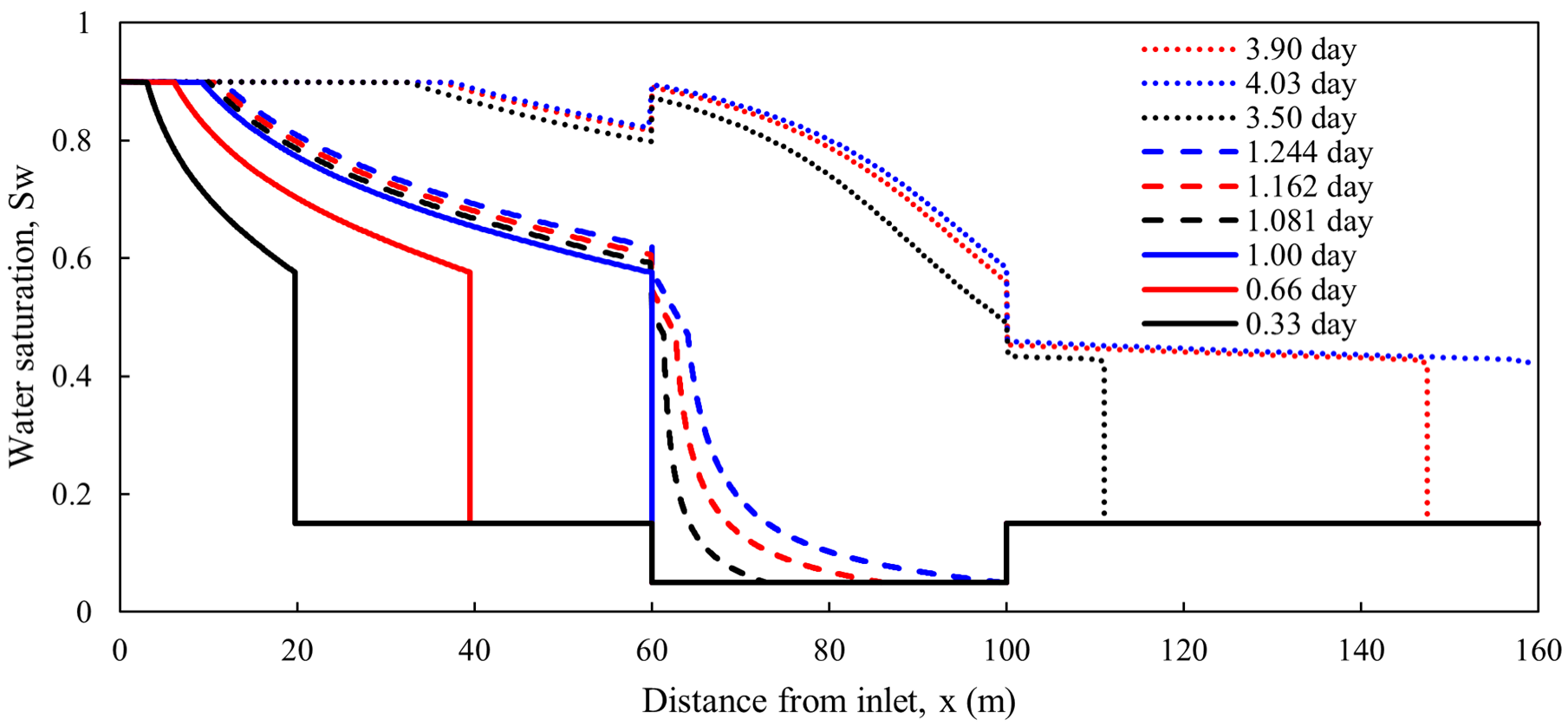
To illustrate the displacement behavior predicted by the filled-cave Forchheimer model under the same PCP geometry, the water-saturation distributions at representative times are shown in Figure 11.

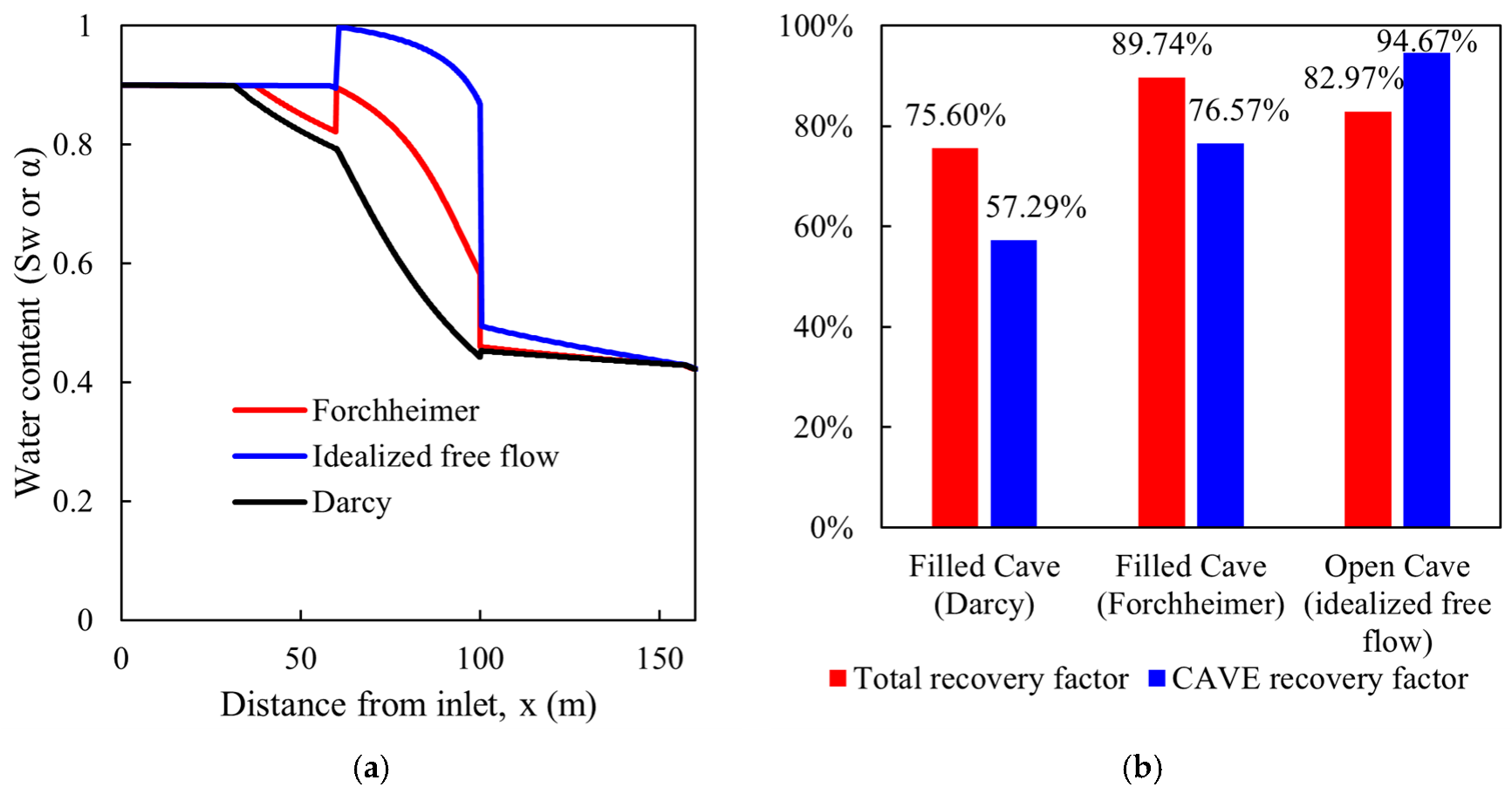
Figure 12a compares the global water-content profiles at the moment when the displacement front reaches the outlet under different cave-flow models. Relative to the open-cave case, the filled-cave Forchheimer model introduces inertial resistance, associated with the packing particles, resulting in a smoother profile and a delayed front advance. Figure 12b compares the recovery factors under the same cave geometry. The open-cave model gives the highest cave recovery (94.67%) but not the highest total recovery (82.97%), suggesting stronger preferential transport and reduced interaction with the surrounding porous domains. By contrast, the Forchheimer filled-cave model yields the highest total recovery (89.74%) and increases the cave recovery from 57.29% in the Darcy filled-cave case to 76.57%. Under the present parameter setting, this result suggests that inertial resistance may weaken short-circuiting and improve the overall recovery.

4. Discussion

The analytical results indicate that the cave mainly acts as a transmission-delay segment between the two porous domains. After the front in PORO1 reaches ${\Gamma }_1$, the upstream fractional flow signal is converted into a water volume fraction signal in the cave and then remapped into the fractional flow relation of PORO2 at ${\Gamma }_2$. Therefore, the downstream front is not a direct continuation of the upstream saturation profile, but is controlled by the constitutive properties of PORO2.

The increase in breakthrough recovery with cave length should be interpreted mainly as a consequence of increased storage capacity and delayed front propagation, rather than as direct evidence of improved microscopic sweep efficiency in the porous matrix. In addition, the comparison of different cave-flow models shows that the open-cave case may yield high local recovery inside the cave but not the highest total recovery, because its high conductivity tends to promote preferential transport. By contrast, the Forchheimer cave weakens short-circuiting and may improve the overall recovery under the present parameter setting. In particular, gravity segregation, capillary redistribution, transverse recirculation, wall-shear effects, and possible turbulent structures inside large caves are neglected in the present formulation. Therefore, the current results should be interpreted as an idealized mechanism-level reference for frontal propagation and interfacial signal transmission, rather than as a full multidimensional prediction for realistic fractured-vuggy reservoirs.

5. Conclusions

In this study, a semi-analytical Buckley–Leverett framework was established for immiscible displacement in a one-dimensional porous–cavernous–porous composite system. The main conclusions are as follows:

(1)

The displacement process in the PCP system is characterized by interface-controlled signal remapping. The front in PORO2 is not a direct continuation of the upstream saturation profile, but is determined by the delayed cave signal and the constitutive relation of the downstream porous medium.

(2)

The cave mainly acts as a transmission-delay and storage segment. Under the present parameter setting, increasing the cave length delays front propagation and increases the recovery factor at breakthrough.

(3)

The internal flow mechanism of the cave significantly affects the system-scale displacement response. Compared with the open-cave case, the Forchheimer cave introduces inertial resistance, delays front advance, and may improve the overall recovery by weakening preferential transport.

(4)

The proposed framework provides an idealized analytical benchmark for understanding front propagation, interface remapping, and recovery behavior in composite vuggy systems under one-dimensional conditions.

References

1. Vidotto, E.; Helmig, R.; Schneider, M.; Wohlmuth, B. Streamline Method for Resolving Sharp Fronts for Complex Two-Phase Flow in Porous Media. Comput. Geosci. 2018, 22, 1487–1502. [Google Scholar] [CrossRef]
2. Jayasinghe, S.; Darmofal, D.L.; Galbraith, M.C.; Burgess, N.K.; Allmaras, S.R. Adjoint Analysis of Buckley-Leverett and Two-Phase Flow Equations. Comput. Geosci. 2018, 22, 527–542. [Google Scholar] [CrossRef]
3. Peng, Y.; Zhang, Y.; Zhang, M.; Ju, B.; Pang, C.; Xu, D. Analytical Solution of Oil and Water Two-Phase Buckley-Leverett Equation in Inclined Stratified Heterogeneous Reservoirs. Geoenergy Sci. Eng. 2025, 251, 213849. [Google Scholar] [CrossRef]
4. Zhang, X.; Shapiro, A.; Stenby, E.H. Gravity Effect on Two-Phase Immiscible Flows in Communicating Layered Reservoirs. Transp. Porous Media 2012, 92, 767–788. [Google Scholar] [CrossRef]
5. Wang, Y.; Xie, P.; Zhang, H.; Liu, Y.; Yang, A. Fracture-Vuggy Carbonate Reservoir Characterization Based on Multiple Geological Information Fusion. Front. Earth Sci. 2024, 11, 1345028. [Google Scholar] [CrossRef]
6. Chen, Z.; Zhang, D.; Li, J.; Hui, G.; Zhou, R. Prediction of Production Indicators of Fractured-Vuggy Reservoirs Based on Improved Graph Attention Network. Eng. Appl. Artif. Intell. 2024, 129, 107540. [Google Scholar] [CrossRef]
7. Wang, Q.; Jiang, H.; Wang, S.; Wang, D.; Bao, R.; Zhang, J.; Li, J. A Novel Method for Modeling Oil-Water Two-Phase Flow in Fractured-Vuggy Carbonate Reservoirs Considering Fluid Vertical Equilibrium Mechanism. J. Pet. Sci. Eng. 2022, 216, 110753. [Google Scholar] [CrossRef]
8. Chen, S.; He, Y.; Luo, R.; Wang, Z.; Wang, M.; Liu, G.; Chi, L.; Li, H.; Ding, X. A Three-Dimensional Precise Geological Model of Ultra-Deep Carbonate Fault-Controlled Reservoirs Based on Multi-Level Simulation. J. Eng. Res. 2026, 14, 1193–1203. [Google Scholar] [CrossRef]
9. Buckley, S.E.; Leverett, M.C. Mechanism of Fluid Displacement in Sands. Trans. AIME 1942, 146, 107–116. [Google Scholar] [CrossRef]
10. Kaasschieter, E.F. Solving the Buckley–Leverett Equation with Gravity in a Heterogeneous Porous Medium. Comput. Geosci. 1999, 3, 23–48. [Google Scholar] [CrossRef]
11. Guérillot, D.; Kadiri, M.; Trabelsi, S. Buckley–Leverett Theory for Two-Phase Immiscible Fluids Flow Model with Explicit Phase-Coupling Terms. Water 2020, 12, 3041. [Google Scholar] [CrossRef]
12. Pasquier, S.; Quintard, M.; Davit, Y. Modeling Two-Phase Flow of Immiscible Fluids in Porous Media: Buckley-Leverett Theory with Explicit Coupling Terms. Phys. Rev. Fluids 2017, 2, 104101. [Google Scholar] [CrossRef]
13. Wu, Y.-S.; Pruess, K.; Chen, Z.X. Buckley-Leverett Flow in Composite Porous Media. SPE Adv. Technol. Ser. 1993, 1, 36–42. [Google Scholar] [CrossRef]
14. Andreianov, B.; Cancès, C. Vanishing Capillarity Solutions of Buckley–Leverett Equation with Gravity in Two-Rocks’ Medium. Comput. Geosci. 2013, 17, 551–572. [Google Scholar] [CrossRef]
15. Kao, C.-Y.; Kurganov, A.; Qu, Z.; Wang, Y. A Fast Explicit Operator Splitting Method for Modified Buckley–Leverett Equations. J. Sci. Comput. 2015, 64, 837–857. [Google Scholar] [CrossRef]
16. Abushaikha, A.; Guérillot, D.; Kadiri, M.; Trabelsi, S. Buckley–Leverett Theory for a Forchheimer–Darcy Multiphase Flow Model with Phase Coupling. Math. Comput. Appl. 2021, 26, 60. [Google Scholar] [CrossRef]
17. Gao, J.; Zhang, H.; Cai, Z.; Li, H.; Wang, N. Research Progress on the Filling Effect of Paleokarst Caves in Carbonate Fracture-Cave Reservoirs: A Case Study of Tahe Oilfield. Pet. Sci. Bull. 2025, 10, 326–341. [Google Scholar] [CrossRef]
18. Yue, S.; Guo, W.; Ding, M.; Li, A. Improving Recovery Mechanism Through Multi-Well Water and Gas Injection in Underground River Reservoirs. Processes 2025, 13, 2743. [Google Scholar] [CrossRef]
19. Shi, W.; Wang, G.; Rong, S.; Qin, J.; Chen, J.; Tao, L.; Bai, J.; Xu, Z.; Zhu, Q. Pressure Transient Analysis for Vertical Well Drilled in Filled-Cave in Fractured Reservoirs. Fluids 2025, 10, 324. [Google Scholar] [CrossRef]
20. Pan, Y.; Liu, X.; Yang, Z.; Sun, Y.; Chen, C.; Sun, L. Study on the Stabilization Mechanism of Gas Injection Interface in Fractured-Vuggy Reservoirs. Energies 2025, 18, 1996. [Google Scholar] [CrossRef]
21. Li, K.; Horne, R.N. Comparison of Methods to Calculate Relative Permeability from Capillary Pressure in Consolidated Water-wet Porous Media. Water Resour. Res. 2006, 42, 2005WR004482. [Google Scholar] [CrossRef]
22. Torabi, F.; Mosavat, N.; Zarivnyy, O. Predicting Heavy Oil/Water Relative Permeability Using Modified Corey-Based Correlations. Fuel 2016, 163, 196–204. [Google Scholar] [CrossRef]
23. Ding, Y.; Zhang, Q.; Xiang, W.; Wang, B.; Lyu, X.; Zhang, L. Stability Analysis of Cavern Collapse in Fractured-Cavity Oil Reservoirs. Sustainability 2023, 15, 6809. [Google Scholar] [CrossRef]
24. Liu, S.; Zhang, Y.; Du, H.; Liu, J.; Zhou, Z.; Wang, Z.; Huang, K.; Pan, B. Experimental Study on Fluid Flow Behaviors of Waterflooding Fractured-Vuggy Oil Reservoir Using Two-Dimensional Visual Model. Phys. Fluids 2023, 35, 062106. [Google Scholar] [CrossRef]
25. Lapponi, F.; Casini, G.; Sharp, I.; Blendinger, W.; Fernández, N.; Romaire, I.; Hunt, D. From Outcrop to 3D Modelling: A Case Study of a Dolomitized Carbonate Reservoir, Zagros Mountains, Iran. Pet. Geosci. 2011, 17, 283–307. [Google Scholar] [CrossRef]
26. Wu, Y. Non-Darcy Displacement of Immiscible Fluids in Porous Media. Water Resour. Res. 2001, 37, 2943–2950. [Google Scholar] [CrossRef]
27. Li, D.; Engler, T.W. Literature Review on Correlations of the Non-Darcy Coefficient. In Proceedings of the SPE Permian Basin Oil and Gas Recovery Conference; SPE: Midland, TX, USA, 2001; p. SPE-70015-MS. [Google Scholar]
28. Elsanoose, A.; Abobaker, E.; Khan, F.; Rahman, M.A.; Aborig, A.; Butt, S.D. Estimating of Non-Darcy Flow Coefficient in Artificial Porous Media. Energies 2022, 15, 1197. [Google Scholar] [CrossRef]
29. Zhu, Z.; Kang, Z.; Chen, H.; Wu, F.; Wang, L.; Wang, B.; Wei, P.; Hou, H. Analysis of the Filling Patterns and Reservoir Development Models of the Ordovician Paleokarst Reservoirs in the Tahe Oilfield. Mar. Pet. Geol. 2024, 161, 106690. [Google Scholar] [CrossRef]
30. Amiri, L.; Ghoreishi-Madiseh, S.A.; Hassani, F.P.; Sasmito, A.P. Estimating Pressure Drop and Ergun/Forchheimer Parameters of Flow through Packed Bed of Spheres with Large Particle Diameters. Powder Technol. 2019, 356, 310–324. [Google Scholar] [CrossRef]
31. Lenci, A.; Zeighami, F.; Di Federico, V. Effective Forchheimer Coefficient for Layered Porous Media. Transp. Porous Media 2022, 144, 459–480. [Google Scholar] [CrossRef]
32. Wang, Y.; Gao, X.; Zhang, Y.; Song, Y.; Wang, H.; Qu, F. Epigenetic Karst in Carbonate Buried Hills and Its Influence on Reservoir Development: A Case Study of the Carboniferous Weixi’nan Sag, Beibuwan Basin, China. Energy Explor. Exploit. 2024, 42, 1505–1534. [Google Scholar] [CrossRef]
33. Zhang, H.; Xu, G.; Liu, M.; Wang, M. Formation Environments and Mechanisms of Multistage Paleokarst of Ordovician Carbonates in Southern North China Basin. Sci. Rep. 2021, 11, 819. [Google Scholar] [CrossRef] [PubMed]
34. Hassan, E.B.E.; Hoffmann, J. Review on Pressure Drop through a Randomly Packed Bed of Crushed Rocks. Discov. Appl. Sci. 2024, 6, 126. [Google Scholar] [CrossRef]
35. Hoffmann, J.; Manatsa, T.; Houtappels, J. Flow Resistance of Randomly Packed Beds of Crushed Rock and Ellipsoidal Particles Using CFD. J. Fluid Flow Heat Mass Transf. 2022, 9, 10–22. [Google Scholar] [CrossRef]
Figure 1. Schematic of the one-dimensional porous–cavernous–porous geometry.
Energies 19 02463 g001
Figure 2. Control volume at interface Γ1.
Energies 19 02463 g002
Figure 3. Two-phase flow transport properties in PORO1 and PORO2. (a) Relative permeability curves; (b) fractional flow function; (c) derivative of the fractional flow function.
Energies 19 02463 g003
Figure 4. Stage-wise front propagation across PORO1, CAVE, and PORO2. (a) Water-saturation profiles in PORO1 before arrival at Γ1; (b) water volume fraction profiles in the cave during transit from Γ1 to Γ2; (c) water-saturation profiles in PORO2 after entry at Γ2.
Energies 19 02463 g004
Figure 5. Remapping of the characteristic front state across PORO1, CAVE, and PORO2.
Energies 19 02463 g005
Figure 6. Water-content profiles for different cave lengths at selected front-arrival moments. (a) Front arrival at the interface Γ2; (b) front arrival at the outlet.
Energies 19 02463 g006
Figure 7. Effect of cave-length ratio on average front advance rates and recovery factor at breakthrough.
Energies 19 02463 g007
Figure 8. Fractional flow functions and their derivatives in PORO1 and PORO2 under different non-Darcy constants. (a) Water fractional flow function; (b) derivative of the water fractional flow function.
Energies 19 02463 g008
Figure 9. Characteristic water content profiles at specific front positions. (a) Front arrival at the interface Γ1; (b) front arrival at the interface Γ2; (c) front arrival at the outlet.
Energies 19 02463 g009
Figure 10. Recovery factors of the PCP system and its individual segments under different non-Darcy constants. (a) Total recovery factor; (b) PORO1 recovery factor; (c) CAVE recovery factor; (d) PORO2 recovery factor.
Energies 19 02463 g010
Figure 11. Water-saturation profiles at representative times for the filled-cave Forchheimer model.
Energies 19 02463 g011
Figure 12. Comparison of displacement profiles and recovery factors under different cave-flow models. (a) Water-content profiles when the front reaches the outlet; (b) total recovery factor and cave recovery factor.
Energies 19 02463 g012