Optimizing High-Resolution CSP–PV Hybrid Power Plant Configurations for Morocco: A Techno-Economic Study

Abstract

Hybridizing concentrating solar power (CSP) with photovoltaics (PV) offers a pathway to combine low-cost daytime generation with dispatchable nighttime supply. This study compares two CSP–PV hybridization concepts for Midelt, Morocco, under a common tender-style design framework: (i) a co-located configuration in which PV and CSP interact at the grid level and (ii) an EH-integrated configuration in which an electric heater (EH) uses PV electricity to heat molten salt in a topping cycle. The main contribution of this study lies in the two-stage optimization workflow, in which leading candidates are selectively re-simulated at higher temporal resolution. This workflow is applied to a common design framework that compares EH-integrated and co-located concepts while considering multiple PV technologies and a broad set of interdependent sizing variables. A surrogate-assisted genetic algorithm evaluates more than 200,000 candidate designs across PV technology, inverter size, TES capacity, EH capacity, and battery energy storage system (BESS) size. The optimization minimizes the levelized cost of energy (LCOE) subject to a $200 {\mathrm{MW}}_{\mathrm{el}}$ export limit, a CAPEX ceiling, and a nighttime-delivery constraint of ${\mathrm{CF}}_{\mathrm{night}}\ge 39\%$. Candidate designs are screened at 600 s and selectively re-simulated at 120 s, showing that temporal refinement affects not only KPI values but also candidate feasibility, final ranking, and preferred component sizing. The lowest-LCOE solution is the EH-integrated bifacial configuration, achieving 64.5% overall capacity factor, ${\mathrm{CF}}_{\mathrm{night}}=39.1\%$, less than 0.1% curtailment, a specific CAPEX of $4698/kW, and an LCOE of 7.29 ¢/kWh. Pareto-front and parameter-trend analyses further show that stricter nighttime-delivery targets shift the dominant sizing levers and define a neighborhood of near-optimal solutions rather than a single fixed design.

1. Introduction

1.1. Background and Motivation

According to the International Renewable Energy Agency (IRENA), the global share of renewable energy (RE) in installed electricity capacity increased from 28.2% in 2014 to 43% in 2023 [1]. As these technologies mature—improving in performance and declining in cost—opportunities to exploit synergies and address grid stability also increase, allowing combinations of different RE technologies to offset one another’s weaknesses. In principle, the hybridization of renewable systems is possible across the technology spectrum; some pairings, however, are particularly natural.

More than a decade ago, Platzer (2014) proposed that combining photovoltaic (PV) and concentrating solar power (CSP) could capitalize on low-cost daytime PV generation while using CSP with thermal energy storage (TES) to shift energy to the night [2]. Today, CSP–PV hybridization is no longer merely a research concept: multiple commercial projects—such as DEWA IV, Cerro Dominador, and several commissioned plants in China (e.g., CNCC Yumen, CTGR Qinghai Golmud, and Three Gorges/CTGR Guazhou)—demonstrate its real-world deployment [3].

The Noor Solar Park in Ouarzazate, Morocco—while not advertised as a hybrid—embeds the foundations of a hybrid system:

• Noor I (2015): 160 MW CSP (parabolic trough collector, PTC) with 3 h of storage.
• Noor II (2018): 200 MW CSP (PTC) with 7 h of storage.
• Noor III (2018): 150 MW CSP (central receiver system, CRS) with 7 h of storage.
• Noor IV (2018): 72 MW PV plant.

Based on the experience of these installations, local authorities announced plans for an 800 MW hybrid CSP–PV complex, “Noor Midelt I,” located roughly 400 km to the northeast near the city of Midelt, Morocco. The 2017 Noor Midelt guidelines outline two hybrid plants. Each should include 150–190 MW of CSP with at least 5 h of thermal storage, up to 300 MW of PV, and a grid connection between 180 and 228 MW. The target average annual generation is 943 GWh, with an investment budget of $1.149 billion (2017) [4]. To the authors’ knowledge, although a contract has been awarded, construction has not yet started [5].

The design and evaluation of large solar parks such as Noor Ouarzazate and Noor Midelt are therefore important not only for project development, but also for improving the simulation and optimization tools used to assess future hybrid systems. As these plants come online and performance data become available, researchers can refine simulation models to better understand and improve complex hybrid systems, informing the next generation of projects.

1.2. CSP Technology

CSP and PV are both solar technologies, but they operate on fundamentally different principles. CSP uses reflective surfaces (mirrors) to concentrate solar irradiance on a focal area, heating a heat transfer fluid (HTF) that is converted to electricity via a thermomechanical process. This heat can be stored in a thermal energy storage (TES) system. As Zhang et al. (2013) note, the key benefit of CSP is its ability to leverage TES and operate as a dispatchable, flexible resource, supplying heat or electricity on demand over short to long durations [6].

CSP optical configurations are often categorized as line-focus and point-focus. Line-focus systems concentrate radiation along a line in a 2D plane, whereas point-focus systems concentrate onto a single point in 3D. In practice, line-focus technologies include parabolic trough collectors, and 64 utility-scale PTC plants are in operation worldwide [7]. PTC plants remain the most common CSP technology, primarily due to their technological maturity [8].

1.3. PV + Battery Energy Storage Systems (BESSs)

PV technology relies on the photovoltaic effect, in which absorbed photons in a semiconductor (e.g., silicon) generate an electric current. PV technology has improved in recent years due to advances in module efficiency (e.g., bifacial designs) and reductions in installation and tracking costs. IRENA (2024) reports that installed PV costs decreased from $5310/kW in 2010 to $758/kW in 2023 [9].

Utility-scale battery energy storage systems (BESSs) expanded from 0.1 GWh in 2010 to 89 GWh in 2023 [9], typically offering 2–6 full-load hours [10]. This rapid deployment reflects declining system costs, technological advances, fast charge and dispatch capabilities, and compatibility with various RE systems [9,10,11,12].

1.4. Review of CSP–PV Hybridization Concepts

Numerous studies explore and build upon CSP hybridization concepts, including early work by Platzer (2014) [2] and Green et al. (2015) [13], those summarized in Table 1, and many others. Collectively, these studies show how hybrid plants can meet contractual capacities, reduce costs, and improve operations.

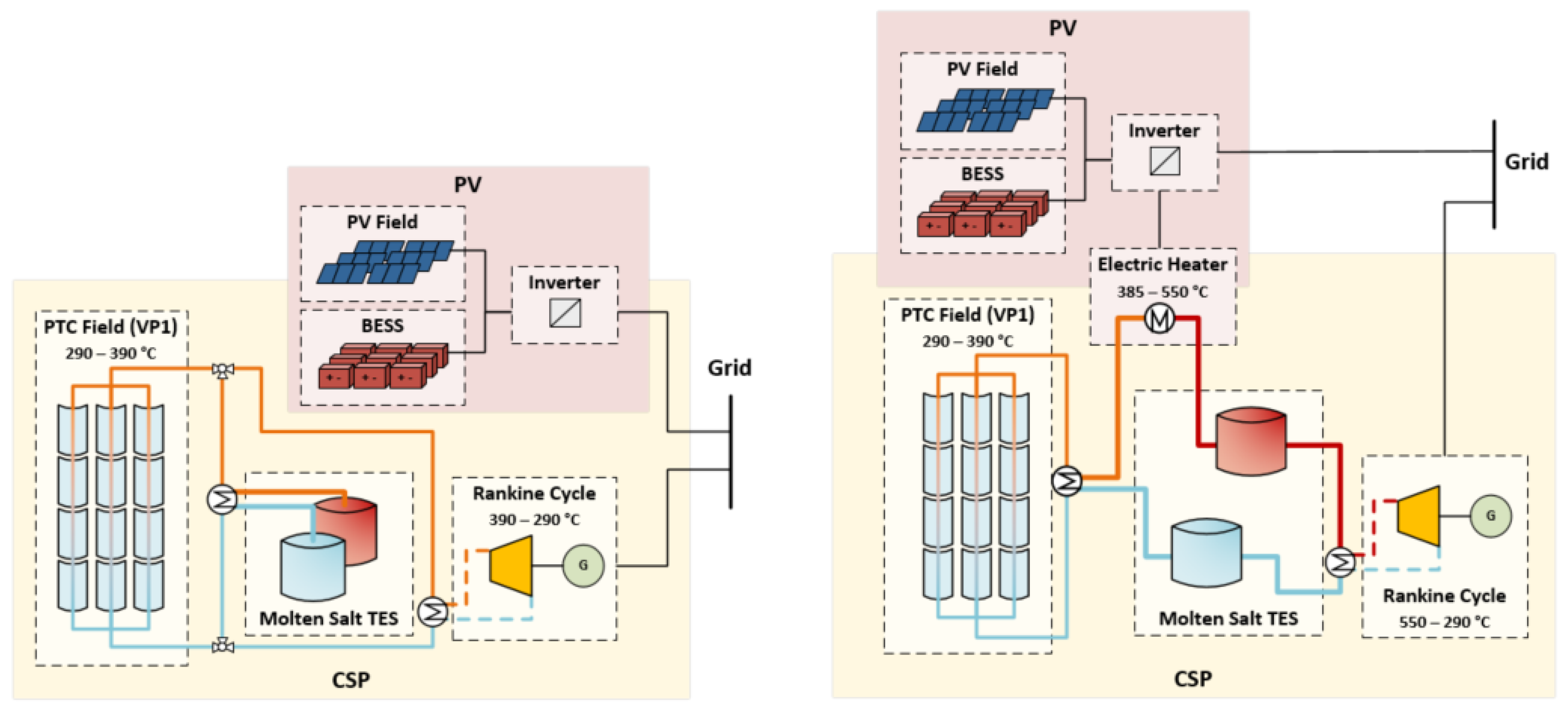
This work distinguishes two categories of hybridization—grid-level and technology-level—as illustrated on the left and right of Figure 1, respectively.

Grid-level hybridization involves independent plants located near each other (“co-located”) that share infrastructure and better satisfy transmission operator requirements. Under a flat-rate power purchase agreement (PPA), for example, the PV plant supplies daytime energy while the TES charges; the TES then discharges to run CSP at night or during cloudy daytime periods. As noted by Green et al. (2015), this approach can yield an annual availability of 98.5% and a capacity factor (CF) of 84.8% [13].

Several studies assume such PPA structures for co-located PTC–PV plants. Starke et al. (2016, 2018) reported a levelized cost of energy (LCOE) of 12–13 ¢/kWh with a CF greater than 80% for Crucero, Chile [14,15], and Bousselamti et al. (2021) reported 9 ¢/kWh with 79% CF in Midelt, Morocco [16]. Benitez et al. (2023) modeled electricity demand in three locations in northern Africa, including fossil generation purchases when hybrid plants could not meet demand [17]. For high-CF PTC (oil) plants, LCOE ranged from 11.0 to 15.2 ¢/kWh and, for high-CF PTC (molten salt, MS) plants, from 10.7 to 12.3 ¢/kWh.

Technology-level hybridization integrates technologies within a single plant so that components are interdependent. For example, Bode et al. (2019) note that a CSP plant can add low-cost PV to offset daytime auxiliary consumption, increasing net CSP delivery under a PPA [18]. For hybrid plants with substantial shares of both PV and CSP, an electric heater (EH) integrated with CSP is a key pathway. The EH can be used within a topping cycle to improve thermal efficiency [19,20,21,22], as an offtaker for cheap or excess electricity [23,24], or as a full replacement for the solar field in a Carnot-battery configuration [25]. The EH can be powered by additional PV capacity, grid purchases, or both.

Table 1. Chronological review of selected optimization studies for hybrid CSP–PV plants.

Study	Year	Simulation Tool	Location	CSP PB (MW)	CSP SF Tech.	EH	PV Tracking	BESS	Optimizer	Opt. Par.	Objective(s)
Petrollese et al. [26]	2016	MATLAB	Ottana (IT), Ouarzazate (MA)	1	LFC (oil, low-T)	No	Fixed	Yes	MILP	5	Min LCOE
Starke et al. [14]	2016	TRNSYS	Crucero (CL)	50	PTC (oil); CRS	No	Fixed	No	Hooke–Jeeves	4	Min LCOE, CF ≥ 80%
Starke et al. [15]	2018	TRNSYS	Crucero (CL)	50	PTC (oil); CRS	No	Fixed	No	NSGA-II	4	Min LCOE, Max CF, Min CAPEX
Guo et al. [25]	2020	MATLAB	Karachi (PK)	100	TES-driven PB	Yes	Fixed	No	MOPSO	3	Min LCOE, Max $R_{\mathrm{ch}}$
Bousselamti et al. [16]	2021	In-house	Midelt (MA)	1–200 (opt.)	PTC (oil)	No	Fixed	No	NSGA-II	4	Min LCOE, Max CF (Min Dump Gen.)
Hassani et al. [27]	2021	SAM	Oujda (MA)	100	CRS	No	Fixed	No	Parametric	2	Min LCOE
Gedle et al. [19]	2022	PCTrough (in-house)	Morocco	100	PTC (oil)	Yes	1-Axis	No	Sweep	4	Min LCOE
Jbaihi et al. [28]	2022	Greenius + SAM	Morocco (south)	50	PTC (oil)	No	Fixed	No	Parametric	2	Min LCOE
Iñigo-Labairu et al. [20]	2022	Greenius	7 sites	20–196	PTC (oil); CRS	Yes	1-Axis	No	Parametric	4	Min LCOE
Benitez et al. [17]	2023	INSEL	Jordan, Tunisia, Algeria	100	PTC (oil/MS); CRS	No	1-Axis	No	Parametric	3	Min LCOE
Guccione et al. [21]	2023	MoSES + PySAM	Évora (PT); Likana (CL)	10/100	PTC (oil/MS); CRS	Yes	1-Axis	No	NSGA-II	5	Min LCOE, Max CF
Pilotti et al. [24]	2023	SAM + Thermoflex	Priolo Gargallo (IT)	21.5 (CSP)	LFC (MS)	Yes	Fixed	Yes	MILP	8	Min LCOE
Mahdi et al. [22]	2024	SPOT	Midelt (MA)	100	PTC (oil)	Yes	Fixed	No	Surrogate + GA	4	Min LCOE

Table 1. Chronological review of selected optimization studies for hybrid CSP–PV plants.

Study	Year	Simulation Tool	Location	CSP PB (MW)	CSP SF Tech.	EH	PV Tracking	BESS	Optimizer	Opt. Par.	Objective(s)
Petrollese et al. [26]	2016	MATLAB	Ottana (IT), Ouarzazate (MA)	1	LFC (oil, low-T)	No	Fixed	Yes	MILP	5	Min LCOE
Starke et al. [14]	2016	TRNSYS	Crucero (CL)	50	PTC (oil); CRS	No	Fixed	No	Hooke–Jeeves	4	Min LCOE, CF ≥ 80%
Starke et al. [15]	2018	TRNSYS	Crucero (CL)	50	PTC (oil); CRS	No	Fixed	No	NSGA-II	4	Min LCOE, Max CF, Min CAPEX
Guo et al. [25]	2020	MATLAB	Karachi (PK)	100	TES-driven PB	Yes	Fixed	No	MOPSO	3	Min LCOE, Max $R_{\mathrm{ch}}$
Bousselamti et al. [16]	2021	In-house	Midelt (MA)	1–200 (opt.)	PTC (oil)	No	Fixed	No	NSGA-II	4	Min LCOE, Max CF (Min Dump Gen.)
Hassani et al. [27]	2021	SAM	Oujda (MA)	100	CRS	No	Fixed	No	Parametric	2	Min LCOE
Gedle et al. [19]	2022	PCTrough (in-house)	Morocco	100	PTC (oil)	Yes	1-Axis	No	Sweep	4	Min LCOE
Jbaihi et al. [28]	2022	Greenius + SAM	Morocco (south)	50	PTC (oil)	No	Fixed	No	Parametric	2	Min LCOE
Iñigo-Labairu et al. [20]	2022	Greenius	7 sites	20–196	PTC (oil); CRS	Yes	1-Axis	No	Parametric	4	Min LCOE
Benitez et al. [17]	2023	INSEL	Jordan, Tunisia, Algeria	100	PTC (oil/MS); CRS	No	1-Axis	No	Parametric	3	Min LCOE
Guccione et al. [21]	2023	MoSES + PySAM	Évora (PT); Likana (CL)	10/100	PTC (oil/MS); CRS	Yes	1-Axis	No	NSGA-II	5	Min LCOE, Max CF
Pilotti et al. [24]	2023	SAM + Thermoflex	Priolo Gargallo (IT)	21.5 (CSP)	LFC (MS)	Yes	Fixed	Yes	MILP	8	Min LCOE
Mahdi et al. [22]	2024	SPOT	Midelt (MA)	100	PTC (oil)	Yes	Fixed	No	Surrogate + GA	4	Min LCOE

Regardless of category, a central challenge is determining the optimal configuration—sizing components to match local meteorology, economics, and demand. In the studies summarized in Table 1, all but two optimized at least three parameters (e.g., TES capacity, CSP solar-field size, PV oversizing). When only a few free parameters are considered, parametric studies can map the design space and identify an optimum.

Some parameters can be tuned prior to optimization to reduce dimensionality (e.g., for fixed-tilt PV, the optimal tilt angle can be pre-computed). However, pre-optimization can mislead for complex systems; for instance, Starke et al. (2016) found that the optimal PV tilt for standalone PV differs from that for hybrid plants, which favor steeper tilts to boost winter generation [14].

As additional parameters (e.g., EH capacity, power-cycle rating, BESS sizing) are introduced, parametric studies become inefficient and algorithmic optimization is required. The appropriate algorithm depends on the objective function. Among the non-parametric studies in Table 1, five different optimization algorithms were used across eight papers. The optimization objective function can be formulated as a single objective (e.g., minimizing LCOE), a multi-objective function (e.g., minimizing LCOE and maximizing CF), or combined, in which a threshold must be met (e.g., minimizing LCOE subject to CF greater than 80%).

The number of individual simulations required in an optimization is often constrained by computational limits (compute power, simulation resources, time). For example, Bousselamti et al. (2021) used NSGA-II with a population of 50 over 150 generations, corresponding to ~7500 simulations for a single run; three operating modes and two optimization scenarios would imply ~45,000 simulations [16]. These requirements escalate further when many scenarios are examined, such as the 27 explored by Guccione et al. (2023) [21].

Time resolution also matters. Zurita et al. (2020) compared high- and low-resolution PV–CSP (CRS) simulations and found that a 60 min resolution required only ~2.5% of the runtime of a 1 min model but overestimated generation by up to 5.95% and consequently underestimated LCOE by 5.41% [29].

Taken together, the reviewed studies show that CSP–PV hybrids can achieve high capacity factors, reduce costs, and satisfy delivery constraints under a range of market assumptions. However, a clear gap remains between the existing literature and the requirements of practical hybrid-plant design. Although several published studies have compared co-located and EH-integrated CSP–PV concepts under varying technical and economic constraints, to the authors’ knowledge, no prior work has simultaneously optimized hybrid configurations with multiple PV technology options under identical constraints while validating the resulting candidate ranking and component sizing at sub-hourly resolution.

The existing literature has generally treated these questions separately: hybridization concepts are usually assessed in isolation, optimization is often limited to a narrower subset of design variables, and temporal-resolution effects are typically examined only for selected cases rather than across a broad design space. As a result, the combined influence of technology composition, design criteria, and temporal resolution on final candidate selection remains insufficiently resolved.

1.5. Objective

Building on the hybridization concepts in Figure 1 and the optimization approaches summarized above, this paper compares co-located and EH-integrated CSP–PV hybrid concepts for a 200 MW_el Midelt case under a common tender-style design framework. The study considers parabolic-trough CSP, three PV technologies, BESS, and electric-heater integration, subject to a fixed export limit, a CAPEX ceiling, and a minimum nighttime-delivery requirement expressed as ${\mathrm{CF}}_{\mathrm{night}}$.

Compared with the studies reviewed in Table 1, the primary contribution of the present work lies in its two-stage optimization workflow, in which broad screening at 600 s temporal resolution is followed by selective re-simulation at 120 s. This framework is applied to a common Midelt design case that compares co-located and EH-integrated concepts, includes multiple PV technology options, uses localized cost assumptions, and jointly optimizes a broad set of coupled sizing parameters.

The objectives are therefore threefold. First, the study evaluates how the two hybridization concepts and the selected PV technologies perform under identical techno-economic and dispatch-oriented constraints. Second, it examines how temporal resolution influences candidate feasibility, final ranking, and component sizing by combining broad optimization at 600 s with selective re-simulation at 120 s. Third, it extends the comparison through Pareto-front analysis to quantify the cost of higher nighttime delivery and to identify parameter-sizing trends and near-optimal solution neighborhoods along that front.

In this way, this paper is not limited to reporting a single optimum for the Midelt case. Rather, it demonstrates how the two-stage workflow enables a practical comparison of competing hybridization concepts and provides a basis for interpreting how nighttime-delivery requirements reshape both the techno-economic tradeoff and the associated component-sizing decisions.

2. Methodology of Component Modeling

The simulations are carried out using ColSim [30], Fraunhofer ISE’s in-house transient thermal systems tool for annual solar–thermal plant simulation. A key feature of ColSim is its plug-flow-based formulation, in which thermodynamic states are stored within each component and updated at each time step (e.g., 120 s). Because ColSim explicitly represents transported thermal states, thermal inertia, and control-driven state changes in the CSP subsystem, the relevant plant dynamics occur on sub-hourly timescales. An hourly time step would smooth short-duration variations in solar input and plant state, thereby reducing the accuracy of temperature profiles, startup and ramp transitions, TES operation, and dispatch-related results.

At each time step, component states are exchanged across the system to coordinate the operation of the PTC solar field (SF), power block (PB), pumps, electric heaters (EHs), and TES. This enables the coupled, high-resolution simulation required for the analysis and optimization of hybrid plants, where efficient operation depends on the continuous interaction of thermal and electrical subsystems.

As detailed below, ColSim was extended to include fixed-tilt and single-axis tracking PV systems with either monofacial or bifacial modules, inverters, BESSs, and an electric heater.

To support reproducibility, this section summarizes (i) the reference CSP model, (ii) PV module, tracking, bifacial, and inverter modeling (including a cross-check against SAM), and (iii) storage and conversion components used in the hybrid simulations.

2.1. Reference CSP Plant

This study builds on the modeling approach of Rohani et al. (2017) and Gomez Garcia et al. (2025), who validated ColSim against an operating parabolic-trough CSP plant [31,32]. The benchmark plant considered here is Noor II in Ouarzazate, Morocco, which has a rated electrical output of 200 MW_el (gross). Since commissioning, design, performance, and cost information for Noor II have been published [7,33], using these sources, a ColSim reference model was developed and used as the baseline for the subsequent optimization.

Where required, the reference model was adapted to ensure consistency with published performance figures. In particular, Noor II is reported as 200 MW_el gross and 152.7 MW_el net (after parasitic consumption) [33]. To reproduce this gross-to-net difference in ColSim, a maximum combined electrical consumption of 33.2 MW_el was assumed for power-block auxiliaries and ACC operation, with the remaining parasitics assigned to solar-field loads (pumping and tracking). Additionally, Noor II uses the SenerTrough2 collector [7], but detailed collector performance data are not public. Therefore, a smaller ET-150 collector is used, and the number of loops is sized to match Noor II’s total PTC aperture area ($1.78 {\mathrm{km}}^2$) [7]. All modifications are summarized in

Table A1. Noor II literature assumptions (Ouarzazate) and corresponding ColSim inputs for Ouarzazate and Midelt. Optimization baseline uses the ColSim Midelt column unless noted.

Parameter	Unit	Reference	ColSim
			Ouarzazate	Midelt
Site information
Location	–	Ouarzazate	Ouarzazate	Midelt
Reference DNI	${\mathrm{kWh/m}}^2$/a	2503 [7]	2741.0 [34]	2535.0 [34]
Coordinates	–	31.067, −6.830	31.008, −6.863 [34]	32.881, −4.715 [34]
Solar field (PTC)
Aperture area	${\mathrm{m}}^2$	1,779,900 [7]	1,778,575
PTC collector	–	SenerTrough2 [7]	Eurotrough-150
PTC row spacing	m	–	17 [31]
PTC cleanliness	%	–	95 [31]
SF loops	–	400	544
Aux. backup heater	${\mathrm{MW}}_{\mathrm{th}}$	–	40
Storage
TES system	–	2-tank indirect [7]	2-tank indirect
TES FLH	FLH	7 [7]	7
TES capacity	${\mathrm{MWh}}_{\mathrm{th}}$	–	4060 (estimated)
Power block
Cycle type	–	Rankine	Rankine
Cooling technology	–	Dry cooling [7]	Dry cooling
Gross power	MWel	200 [33]	200
Net power	MWel	152.7 [33]	153
Efficiency	%	–	38.4 (PTC) [48]
Min. operation	%	–	18 [49]
Annual performance
Annual yield (expected/reported)	GWh	600/697 [7,33]	696.9	650.1
Capacity factor (expected/reported)	%	34/39.78 [7]	40.0	37.0
Specific CAPEX	$/kW	2018: 5596 [7]	2023: 5071.1/3991.4 (CPI-adj.)
LCOE	¢/kWh	2018: 16.0 [7]	2023: 12.33/ 9.88 (CPI-adj.)	2023: 13.22/ 10.60 (CPI-adj.)

.

Meteorological data were taken from Meteonorm v8. This tool provides a synthetic typical meteorological year for the specific site, representing a stochastically generated long-term mean climate based primarily on satellite data [34]. Based on these data, the average annual direct normal irradiance (DNI) for Ouarzazate ($2741 {\mathrm{kWh/m}}^2$/a) is about 10% higher than the annual DNI value reported by cspguru.com ($2503 {\mathrm{kWh/m}}^2$/a) [7], whereas Midelt’s average from Meteonorm ($2535 {\mathrm{kWh/m}}^2$/a) is slightly lower than that of Ouarzazate.

For benchmarking, the adapted ColSim reference model was compared with published Noor II design and annual performance values for Ouarzazate. Because the publicly available benchmark data are limited to plant-level annual indicators, the comparison in

Table 2. Published Noor II benchmark values and corresponding ColSim results for Ouarzazate.

Metric	Unit	Reference Value	ColSim	Deviation [%]
Reference DNI	${\mathrm{kWh/m}}^2$/a	2503 [7]	2741.0 [34]	+9.5
Gross power	${\mathrm{MW}}_{\mathrm{el}}$	200.0 [33]	200.0	0.0
Net power	${\mathrm{MW}}_{\mathrm{el}}$	152.7 [33]	153.0	+0.2
Annual yield (expected)	GWh	600.0 [7]	696.9	+16.2
Annual yield (reported)	GWh	697.0 [33]	696.9	0.0

serves as an annual benchmark rather than a full operational validation.

With the Meteonorm weather data adopted in the model, the simulated annual net electricity yield for Ouarzazate is 696.9 GWh. This value is approximately 16% above the estimated 600 GWh reported in [7], but matches the reported 2019 generation of 697 GWh from [33]. The overestimation relative to the expected yield is consistent with the 9.5% higher DNI in the Meteonorm dataset compared with the cspguru reference. For Midelt, the same reference configuration yields 650.1 GWh.

Given the documented assumptions and the close agreement with the reported Noor II generation, the ColSim reference model is considered suitable for the subsequent optimization study.

Unless stated otherwise, the reference plant denotes the ColSim-adapted Noor II configuration evaluated at the Midelt site; literature Noor II values and the Ouarzazate ColSim case are used only for benchmarking (Table A1).

2.2. PV Module

PV electrical performance is computed using pvlib with a single-diode representation parameterized from manufacturer data. At each time step, the maximum-power-point current and voltage are evaluated as functions of module temperature and effective irradiance.

Irradiance absorption follows Gilman (2015) [35], using the isotropic model for diffuse radiation. Module current ($I_{\mathrm{mp}}$) and voltage ($V_{\mathrm{mp}}$) are computed with the De Soto five-parameter model [36,37].

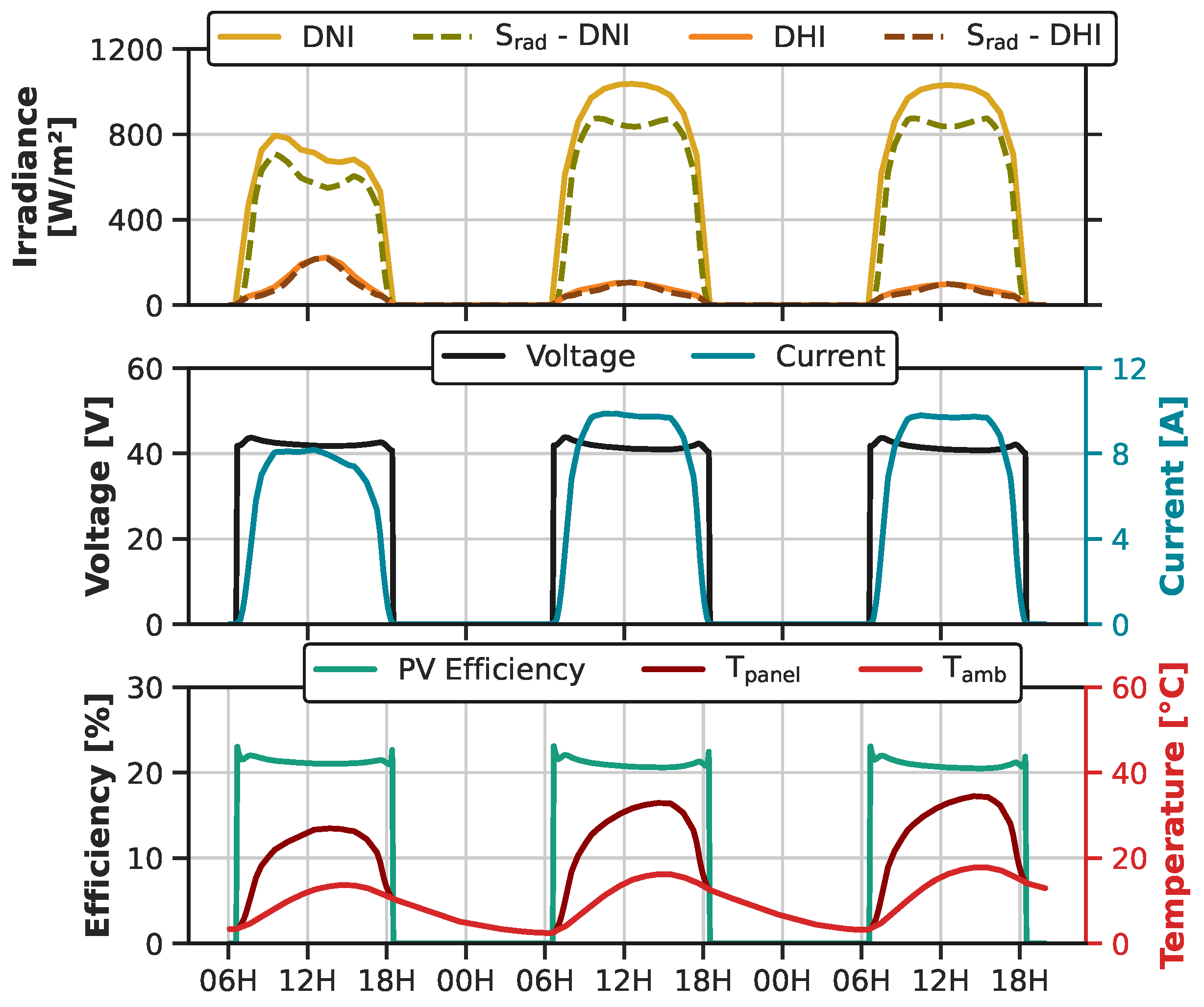
To reduce runtime, the PV module calls a precomputed performance map, returning $I_{\mathrm{mp}}$ and $V_{\mathrm{mp}}$ as functions of total absorbed irradiance $s_{\mathrm{rad},\mathrm{tot}}$ and module temperature $T_{\mathrm{module}}$ at every time step. The maximum-power-point (MPP) efficiency ${\eta }_{\mathrm{mp}}$ follows Equation (1). An example three-day time series is shown in Figure 2.

$$\begin{array}{cc}\hfill {\eta }_{\mathrm{mp}}& ={\displaystyle \frac{I_{\mathrm{mp}}\left(T_{\mathrm{module}},s_{\mathrm{rad},\mathrm{tot}}\right)·V_{\mathrm{mp}}\left(T_{\mathrm{module}},s_{\mathrm{rad},\mathrm{tot}}\right)}{A_{\mathrm{module}}·s_{\mathrm{rad},\mathrm{tot}}}}\hfill \\ \hfill & ·\left(1-{\eta }_{\mathrm{module}\mathrm{loss}}\right)\hfill \end{array}$$

(1)

Module-level losses (e.g., soiling) are applied via ${\eta }_{\mathrm{module}\mathrm{loss}}$, while remaining DC-side losses (e.g., wiring and mismatch) are captured separately through ${\eta }_{\mathrm{field}\mathrm{loss}}$ in Equation (3).

After computing the maximum-power-point efficiency, the module DC power $P_{\mathrm{module}}$ is obtained from Equation (2), adapted from Duffie and Beckman (2013) [37].

$$P_{\mathrm{module}}={\eta }_{\mathrm{mp}}·s_{\mathrm{rad},\mathrm{tot}}·A_{\mathrm{module}}$$

(2)

Manufacturer parameters and additional data were obtained from the SAM database [38]. Key characteristics for monofacial and bifacial modules are listed in

Table 3. Monofacial and bifacial PV module data [38].

Description	Unit	Monofacial	Bifacial
PV Module	–	JA Solar 460	Trina Solar 705 NE
Manufacturer	–	JA Solar Co., Ltd.	Trina Solar Co., Ltd.
Origin	–	Beijing, China	Changzhou, China
Nominal Power Rating	W	459.7	705.3
Technology	–	Mono Si, PERC	Mono Si, TOPCon
Module Area	${\mathrm{m}}^2$	2.17	3.08
Nominal Efficiency	%	21.19	22.9
Transmission Factor	–	–	0.013
Bifaciality	–	–	0.85
Soiling Loss (Module)	%	5.0	5.0
DC Field Loss (Wiring)	%	4.44	4.44
PV Degradation	%/a	0.5	0.5

.

Finally, the PV field DC power $P_{\mathrm{DC}}$ is the product of the per-module output and the number of modules, accounting for field losses as in Equation (3).

$$P_{\mathrm{DC}}=P_{\mathrm{module},\mathrm{out}}·N_{\mathrm{modules}}·\left(1-{\eta }_{\mathrm{field}\mathrm{loss}}\right)$$

(3)

2.3. Single-Axis Tracking

One method to enhance PV plant performance is to incorporate single-axis tracking technology, which rotates PV modules about one axis with a north–south orientation to reduce cosine losses, thereby increasing yield by roughly 10–20% [39].

As with fixed-tilt systems, partial shading from array geometry and row-to-row interactions can materially reduce output. Shading and related losses are modeled using (i) the row-to-row shading model in [40], (ii) diffuse irradiance reduction [35,41], (iii) ground-reflected diffuse reduction [35,41], and (iv) DC mismatch factors [41]. A ground-coverage ratio (GCR) of 0.3 and a ground albedo of 0.2 are assumed [42].

To balance morning and evening shading, a backtracking algorithm selects at each time step the tracker angle that minimizes inter-row shadowing. A maximum tilt of ${45}^{\circ }$ is assumed.

2.4. Bifacial PV Technology

Bifacial modules absorb irradiance on both front and rear sides. Gains typically rise with latitude, ranging from ~1–12% between $0^{\circ }$ and ${65}^{\circ }$ (and higher over bright ground) [43]. Owing to technological and manufacturing advances, bifacial market share is projected to reach ~70% of utility-scale modules by 2030 [44].

The bifacial modeling follows pvlib’s bifacial module [45], which implements the view-factor approach of Mikofski et al. (2019) [46] to compute front- and rear-side plane-of-array irradiance and absorption. To reflect current market trends, a premium, high-bifaciality module is used (Table 3). The bifacial modules are also modeled with single-axis tracking about a north–south-oriented axis.

2.5. Inverter Technology

The inverter converts PV field DC power ($P_{\mathrm{DC}}$) to grid-compatible AC power ($P_{\mathrm{AC}}$) with efficiency ${\eta }_{\mathrm{Inv}}$ (Equation (4)). A constant inverter efficiency of 98.5% is assumed.

$$P_{\mathrm{AC}}=P_{\mathrm{DC}}·{\eta }_{\mathrm{Inv}}$$

(4)

The inverter has a maximum AC rating $P_{\mathrm{AC},\max }$. Excess DC input results in “clipping,” i.e., AC output that is shed:

$$\begin{array}{cc}\hfill \mathrm{If}{P}_{\mathrm{AC}}& >P_{\mathrm{AC},\max },\mathrm{then}\hfill \end{array}$$

(5)

$$\begin{array}{cc}\hfill P_{\mathrm{Shed}}& =P_{\mathrm{DC}}·{\eta }_{\mathrm{Inv}}-P_{\mathrm{AC},\max }\hfill \end{array}$$

(6)

$$\begin{array}{cc}\hfill P_{\mathrm{AC}}& =P_{\mathrm{AC},\max }\hfill \end{array}$$

(7)

For steady delivery, the PV field is oversized relative to the inverter rating; typical standalone sizing uses $R_{DC/AC}=P_{\mathrm{DC},\mathrm{nom}}/P_{\mathrm{AC},\mathrm{nom}}\approx 1.05$–1.20.

2.6. Cross-Checking of PV and Inverter Modeling

NREL’s open-source System Advisor Model (SAM, v. 2025.4.16) provides a well-documented reference implementation for PV and inverter modeling and was therefore used as a benchmark in this study.

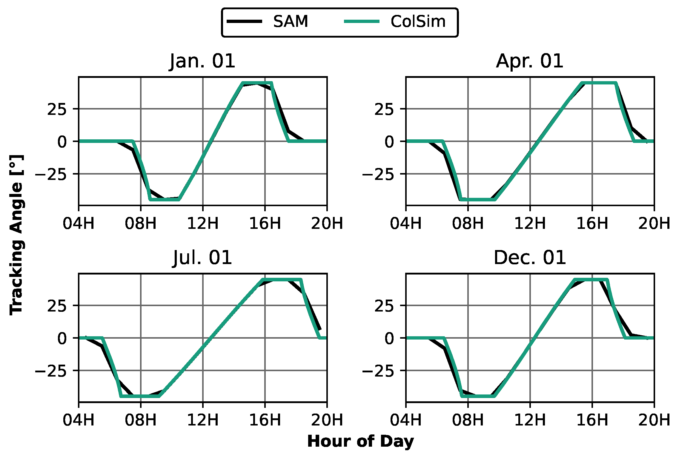
For the annual comparison, a 106.0 MW_DC bifacial PV field is coupled to a 100.1 MW_AC inverter system ($R_{DC/AC}=1.06$), north–south oriented, using the Ouarzazate weather file [34]. The ColSim time step is 120 s. Figure 3 compares single-axis tracking angles for four representative days; ColSim’s curves are smoother due to the finer 120 s time step used here as compared to the 1 h time step in SAM.

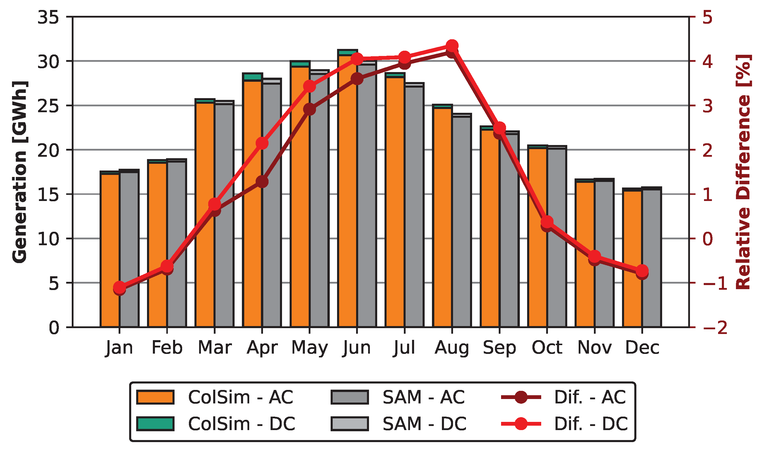
ColSim predicts an annual PV yield of 280.98 GWh_DC, versus 275.66 GWh_DC in SAM (a 1.9% difference). An hourly time-series comparison yields an R² of 0.9951 and an RMSE of 0.0026 GWh for the DC output, confirming excellent agreement between the two models. Remaining differences arise primarily from module-efficiency calculations and the backtracking implementation.

SAM applies a voltage-dependent inverter efficiency, whereas ColSim uses a simplified constant ${\eta }_{\mathrm{Inv}}$. On the AC side, the hourly comparison gives an R² of 0.9954 and an RMSE of 0.0025 GWh. The dark-red trace in Figure 4 shows that monthly AC differences largely track DC differences.

Overall, the comparison shows close agreement in seasonal patterns and monthly energy, supporting the use of the simplified inverter and PV formulations in the hybrid optimization.

2.7. BESS Technology

The BESS formulation follows Zurita et al. (2018) [47]. The battery charges and discharges within bounds defined by depth of discharge (DoD) and state of charge (SOC). A DC–DC Li-Ion system with 80% usable capacity (${\mathrm{SOC}}_{\min }$: 10%, ${\mathrm{SOC}}_{\max }$: 90%) and single-trip efficiency ${\eta }_{c/d}=92\%$ is integrated, giving ~85% round-trip efficiency [10]. The BESS maximum charge/discharge power $P_{\mathrm{c}/\mathrm{d},\max }$ is set to 100 MW, with losses included. The BESS is placed on the DC side (“before” the inverter), so clipped DC can be stored and later discharged. In the optimization, the energy capacity $E_{\mathrm{BESS}}$ is treated as a decision variable (

Table 4. BESS information.

Description	Unit	Value
BESS Technology	–	Li-Ion
Power rating (charge/discharge)	MW	100
Energy capacity	MWh	optimized
Single-Trip Efficiency	%	92
Depth of Discharge	%	80

).

The SOC is updated each time step as in Equation (8) [47]:

$$\begin{array}{cc}\hfill {\mathrm{SOC}}_i& ={\mathrm{SOC}}_{i-1}+{\displaystyle \frac{\Delta t}{E_{\mathrm{BESS}}}}\left({\eta }_c{P}_{\mathrm{ch}}-{\displaystyle \frac{P_{\mathrm{dis}}}{{\eta }_d}}\right)\hfill \end{array}$$

(8)

where $P_{\mathrm{ch}}\ge 0$ and $P_{\mathrm{dis}}\ge 0$ are the charge and discharge power, respectively, ${\eta }_c$ and ${\eta }_d$ are the corresponding efficiencies, and $\Delta t$ is the simulation time step.

2.8. Electric Heater

The molten-salt electric heater is modeled as a simplified heating element that converts electrical input power ($P_{\mathrm{el}}$) into thermal power ($P_{\mathrm{th}}$) with efficiency ${\eta }_{\mathrm{EH}}$ and transfers it directly to the HTF:

$$\begin{array}{cc}\hfill P_{\mathrm{th}}& ={\eta }_{\mathrm{EH}}·P_{\mathrm{el}}\hfill \end{array}$$

(9)

In the present model, the EH raises the molten-salt temperature for the assumed topping-cycle operation. Operational limits include minimum and maximum electrical power ($P_{\mathrm{EH},\min }$ and $P_{\mathrm{EH},\max }$), as well as applied warm-up and cool-down gradients (

Table 5. Electric heater information.

Description	Unit	Value
Minimum Capacity	MW	2
Maximum Capacity	MW	optimized
$\nabla T$ Warm-Up Gradient	°C/min	10
$\nabla T$ Cool-Down Gradient	°C/min	20
Conversion Efficiency	%	99

). Part-load inefficiencies and other detailed performance losses are not considered in this study.

3. Simulation of Hybridization Concepts

For both hybridization concepts, dispatch is evaluated against a constant grid-export setpoint of 200 MW_el, representing a baseload power purchase agreement (PPA). Grid export is limited to 200 MW_el; any instantaneous production above this cap is curtailed.

To make the operational logic explicit, the controller applies the following priority order at each simulation time step:

1.

Supply internal electrical loads (CSP auxiliaries and parasitics, including solar-field pumping/tracking and power-block/ACC auxiliaries),

2.

Export power to the grid to track the 200 MW_el setpoint subject to resource availability and unit constraints,

3.

Operate the BESS within its power and SOC limits to compensate, where possible, for short-term export deficits, including those arising from auxiliary consumption (e.g., power-block and ACC loads),

4.

Allocate remaining PV either to curtailment (co-located case) or to the electric heater (EH-integrated case).

3.1. Co-Located Hybrid Plant

The co-located hybrid plant (Figure 1, left) couples a reference parabolic-trough CSP plant (Section 2.1) with a PV + BESS system at the point of interconnection. In this configuration, PV does not interact thermally with the CSP loop; hybridization occurs at the grid connection through the coordinated dispatch of PV, the BESS, and the CSP power block.

During daytime operation, PV generation first supplies internal electrical loads (CSP auxiliaries and parasitics) and then contributes to meeting the 200 MW_el export setpoint. When PV output exceeds the inverter capacity, the BESS charges up to its power limit and SOC ceiling. If PV generation exceeds auxiliary demand and the export requirement, any remaining surplus is curtailed. When PV output falls below the export setpoint, the BESS may discharge to reduce short-term deviations and smooth ramps, thereby limiting cycling of the CSP power block. Any remaining deficit is supplied by the CSP plant, provided sufficient TES energy is available. If neither TES nor the BESS can cover the shortfall, grid export falls below the setpoint.

At night and during extended cloudy periods, the CSP power block is dispatched up to its nominal output, while the BESS discharges (within its power and SOC limits) to compensate the remaining deficit relative to the export setpoint until the TES is depleted. A minimum hot-salt temperature is enforced to prevent freezing and preserve restart capability. If the hot-tank temperature falls below this threshold, heat tracing is assumed to restore the salt temperature to the minimum operating level. During nighttime operation, the parabolic-trough loop circulates the HTF at a low mass flow; if the HTF temperature drops below a prescribed threshold, backup heating is activated to return it to a safe operating level.

3.2. EH-Integrated Hybrid Plant

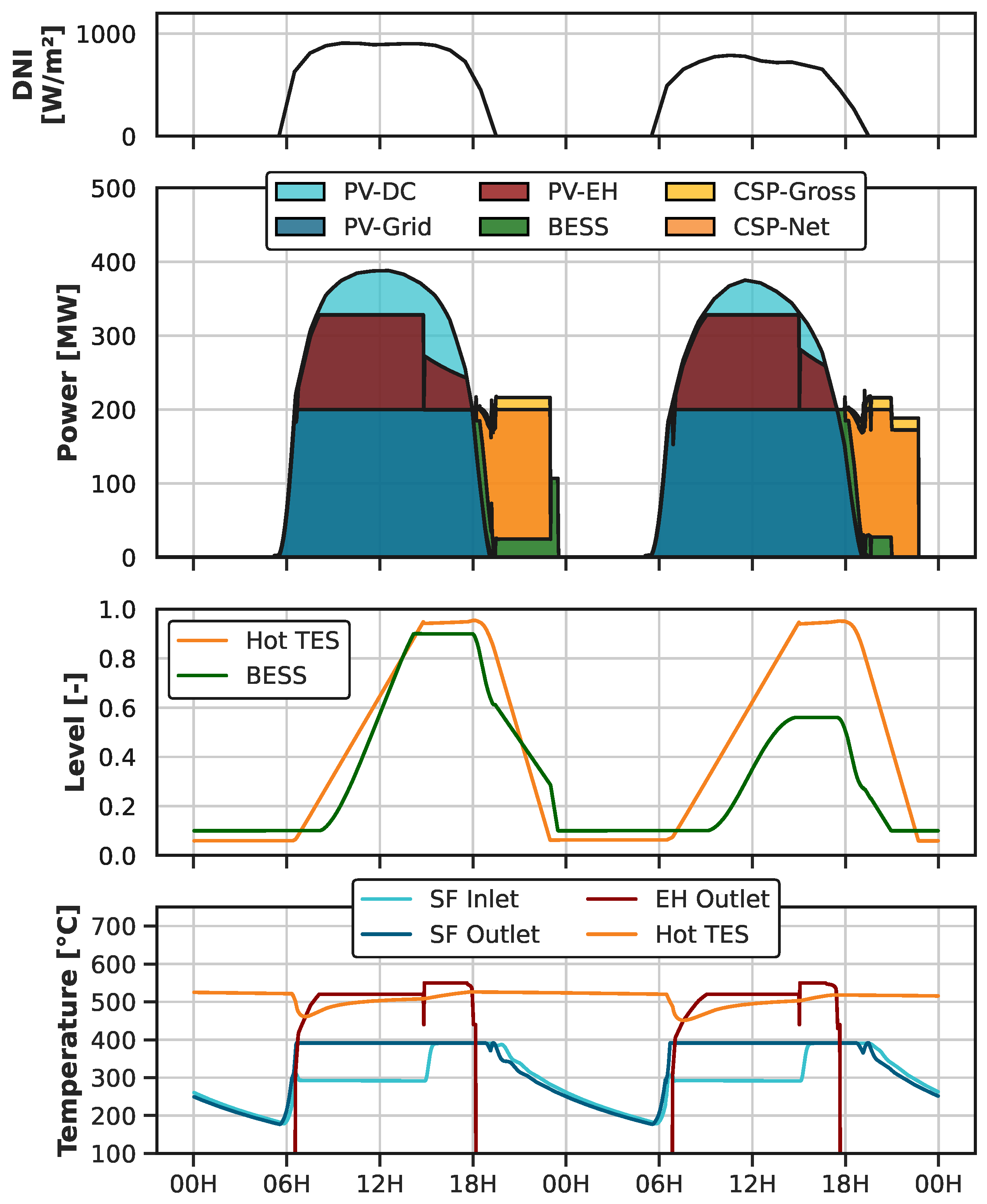
In the EH-integrated configuration (Figure 1, right), the co-located strategy is augmented with an EH supplied by PV. Figure 5 depicts time-series behavior for two representative spring days. The operational logic mirrors the co-located case, where the PV first delivers generation to the CSP auxiliaries (which are small relative to PV output) and then the grid; all remaining generation is sent to the electric heater. The PTC field circulates a synthetic oil HTF between $290 °\mathrm{C}$ and $393 °\mathrm{C}$ (bottoming loop). All available heat is transferred through a heat exchanger to the topping loop, raising the temperature of the molten-salt (MS) HTF exiting the heat exchanger to about $390 °\mathrm{C}$.

The MS then enters the EH, which raises its temperature up to $550 °\mathrm{C}$. Once the setpoint is reached, any surplus electric power is curtailed to avoid overheating. Raising the HTF temperature from $390 °\mathrm{C}$ to $550 °\mathrm{C}$ increases cycle efficiency from 38.4% to 42.8% [48]. The internal auxiliary and ACC cooling requirements were assumed to be reduced to 16.8 MW [49].

The topping-loop control objectives are (i) to absorb all heat from the bottoming loop and (ii) to maximally charge the hot TES tank. Achieving both can require a mass-flow rate through the EH above its design value. In this case, the heater operates at nominal power, but the HTF exits below the design temperature. Consequently, the hot TES may reach full volume while remaining cooler than $550 °\mathrm{C}$.

Because the topping cycle operates at higher thermal-to-electric efficiency and delivers more energy per unit of stored heat, the required hot-tank volume to meet a given night supply is reduced. In this study, the TES is sized by the optimizer to satisfy the nighttime capacity requirement (Section 4.3) rather than a nominal number of full-load hours (FLH) under average conditions.

As shown in the second and fourth subplots of Figure 5, between 16:00 and 18:00, the hot TES is full yet below $550 °\mathrm{C}$ and there is electric generation available, so the HTF is recirculated through the EH until the setpoint is reached.

This strategy mitigates two drawbacks. First, restricting the topping-loop flow to the EH design limit would create a bottleneck and waste daytime solar heat. Second, turbine output is typically more sensitive to inlet mass flow than to inlet temperature; therefore, further charging the TES—even at slightly lower temperature—improves the utilization of both the turbine and the EH, which can continue to operate at nominal capacity during recirculation.

As daytime operation transitions to nighttime and PV output declines, the CSP plant ramps up while the BESS covers the interim gap. In the first nighttime example, CSP operates at nominal conditions and the BESS offsets auxiliary (parasitic) loads, maintaining the constant export setpoint. If TES depletes before the BESS, the BESS then discharges at maximum output until it is empty. In the second nighttime example, the BESS empties before TES/CSP; CSP continues at nominal power, but the export setpoint is no longer fully met.

3.3. Simulation Resolution

All simulations were run on a Linux server (×86_64) with an AMD EPYC 7451 (Advanced Micro Devices, Inc., Santa Clara, CA, USA) and 125 GiB of RAM.

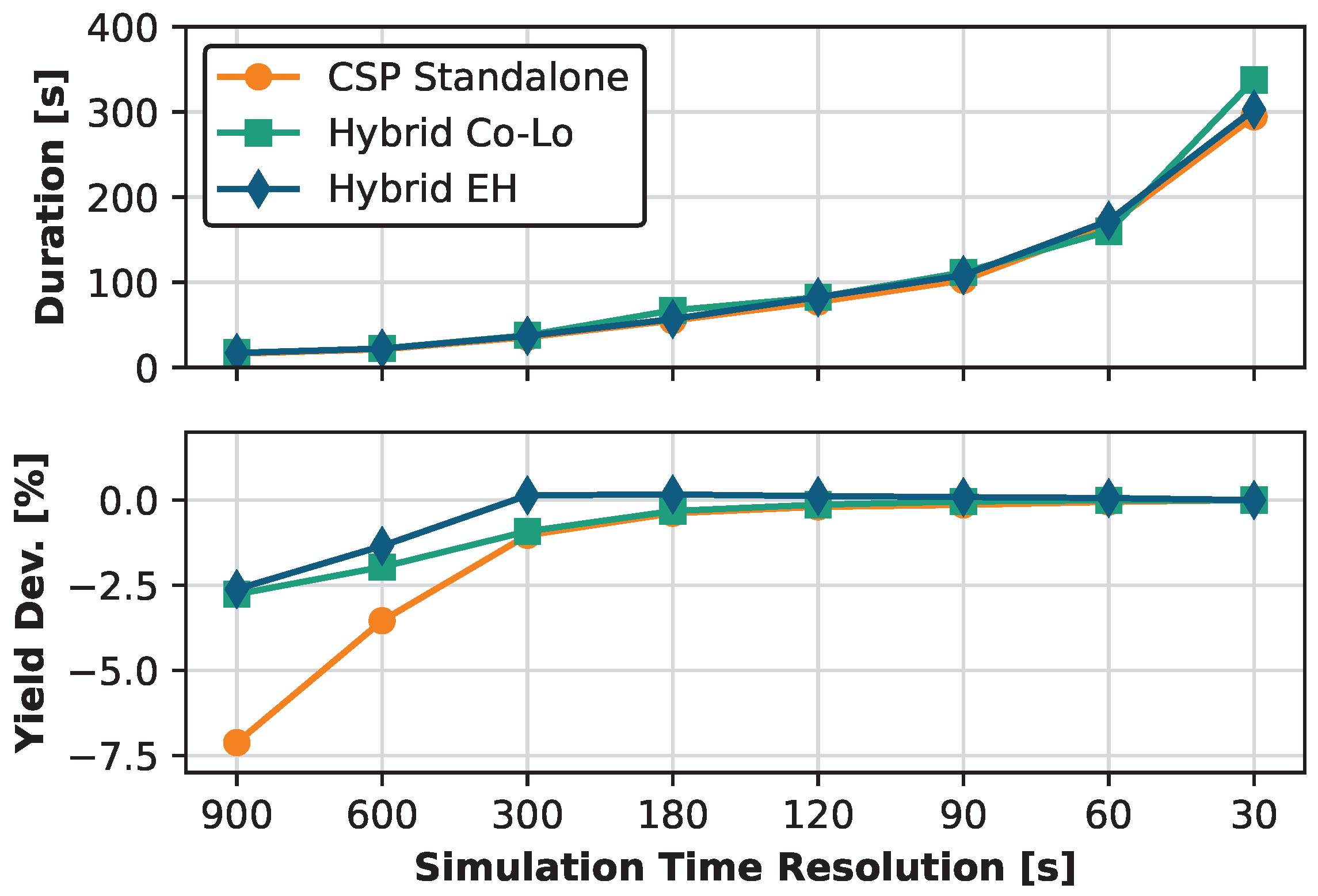
A time-step sensitivity analysis was conducted for three representative configurations—CSP-only, co-located PV–CSP, and EH-integrated—varying the step from 15 min (900 s) to 30 s.

As shown in Figure 6, the wall-clock runtime per annual simulation rose from ~16 s at 15 min resolution to more than 300 s at 30 s resolution. Using the 30 s case as a baseline, the 15 min step underestimated annual net electrical generation by ~7.5% for CSP-only and ~2.5% for the hybrid cases. This discrepancy arises from plug-flow thermal dynamics in the CSP components, whereas PV + BESS is less sensitive to temporal resolution.

4. Techno-Economic and Optimization Approach

This section summarizes the techno-economic modeling and optimization approach for the hybrid subsystems, including cost assumptions (Section 4.1), key performance indicators (Section 4.2), and the optimization framework (Section 4.3). A 25-year lifetime and a real discount rate $r=5\%$ are assumed [16], with 2023 as the cost base year. Detailed technology costs and cost models are provided in Appendix B.

4.1. Cost Assumptions

CSP component costs are adapted from [50], where the referenced component cost takes into account local and country-specific costs (Equation (10)).

$$\begin{array}{c}\hfill C_{\mathrm{comp}}=C_{2023}\left(1-f_{\mathrm{local}}\right)+C_{2023}{f}_{\mathrm{local}}{f}_{\mathrm{country}}\end{array}$$

(10)

The local factor $f_{\mathrm{local}}$ and the country price index $f_{\mathrm{country}}$ were taken from [50]. Costs were inflated to 2023 by 18% relative to 2018 based on local data [51].

Table A2. Cost assumptions for CSP components, assuming an $f_{country}$ of 0.42 [50].

	Unit	2018 Cost	2023 Cost	${\mathit{f}}_{\mathbf{local}}$ %	Adj. Cost
Site Preparation ($c_{\mathrm{site}\mathrm{prep}}$)	${\mathrm{\$/m}}^2$	$25.0	$29.5	90.0%	$14.1
Solar Field ($c_{\mathrm{SF}}$)	${\mathrm{\$/m}}^2$	$127.2	$150.0	51.7%	$105.1
HTF ($c_{\mathrm{HTF}}$)	${\mathrm{\$/m}}^2$	$51.5	$60.8	25.6%	$51.8
TES (Indirect) ($c_{\mathrm{TES},\mathrm{Ind}.}$)	$/kWhth	$40.0	$47.2	21.9%	$41.2
TES (Direct) ($c_{\mathrm{TES},\mathrm{Dir}.}$)	$/kWhth	$26.4	$31.2	34.7%	$24.9
Power Block (VP1) ($c_{\mathrm{PB},\mathrm{VP}1}$)	$/kWel	$920.0	$1085.6	26.5%	$918.7
Power Block (MS) ($c_{\mathrm{PB},\mathrm{MS}}$)	$/kWel	$970.0	$1144.6	26.5%	$968.7
Aux. Backup Heater ($c_{\mathrm{aux}}$) [49]	$/kWth	$40.0	$59.0	26.5%	$49.9

summarizes base costs, inflation adjustments, and local factors;

Table A3. Cost assumptions for the CSP O&M and soft costs.

	Unit	Value	Source
Solar Field ($f_{\mathrm{SF}}$)	% of Total SF Cost	0.5%	[49]
TES ($f_{\mathrm{TES}}$)	% of TES Cost	0.3%	[49]
Power Block ($f_{\mathrm{PB}}$)	% of PB Cost	1%	[49]
Raw Water ($f_{\mathrm{water}}$)	${\mathrm{\$/m}}^3$	0.6 *	[49]
Fuel Price ($f_{\mathrm{fuel}}$)	$/MWhth	33.0 *	[49]
Contingencies ($f_{\mathrm{cont}}$)	% of Comp. Cost	7%	[61]
EPC Cost ($f_{\mathrm{EPC}}$)	% of EPCDirect	11%	[61]
Utility Cost	-	$14.2 * Mil	[49]
Staff ($N_{\mathrm{staff}}$)	-	81	[33]
Admin ($f_{\mathrm{admin}}$)	% of EPCdir	0.15%	[49]
Insurance ($f_{\mathrm{ins}}$)	% of PB	0.3%	[49]
O&M Staff ($f_{\mathrm{staff}}$)	$/year/Person	$47,200 *	[49]
Consumables ($f_{\mathrm{cons}}$)	$/kWhel	1.2 *	[49]

Note: * Denotes adjusted to 2023 costs.

lists O&M and soft costs.

To assess three PV options (fixed-tilt, single-axis, and single-axis bifacial), component costs in

Table A5. Cost assumptions for PV and BESS.

	Unit	Value	Source
Mainstream Module ($c_{\mathrm{module}}$)	$/kWDC	150	[62]
Bifacial Premium ($c_{\mathrm{bifacial}}$)	$/kWDC	10	[62]
BOS ($c_{\mathrm{bos}}$)	$/kWDC	220	[9]
Tracking Premium ($c_{\mathrm{tracking}}$)	$/kWDC	50	[63]
PV Installation ($c_{\mathrm{install}}$)	$/kWDC	110	[9]
Inverter ($c_{\mathrm{inv}}$)	$/kWAC	36.7	[9]
PV Fixed O&M ($c_{\mathrm{PV}\mathrm{O\&M}}$)	$/kWDC/year	7.0	[9]
BESS Storage Capacity (Cstore)	$/kWheffective	168	[64]
BESS Power Capacity (CP)	$/kW	240	[64]
BESS Fixed O&M ($c_{\mathrm{BESS}\mathrm{O\&M}}$)	% of $C_P$	2.5%	[10]
EPC + Overhead ($f_{\mathrm{EPC}}$)	% of Comp. Cost	10%	[9,64]
Contingency ($f_{\mathrm{Cont}}$)	% of Total CAPEX	5%	[21,64,65]

are primarily extrapolated from [9]. Since a published Morocco-specific utility-scale PV cost breakdown was not available in [9], the detailed breakdown for Saudi Arabia was adopted as a regional proxy. It was selected because it is the only Middle East and North Africa case reported therein with a transparent component-level breakdown.

The BESS cost $C_{\mathrm{BESS}}$ depends on the effective energy capacity $E_{\mathrm{BESS}}$ and power rating $P_{\mathrm{BESS}}$ [52]:

$$\begin{array}{cc}\hfill C_{\mathrm{BESS}}& =c_{\mathrm{size}}{E}_{\mathrm{BESS}}+c_{\mathrm{rate}}{P}_{\mathrm{BESS}}\hfill \end{array}$$

(11)

A 15-year battery lifetime is assumed, with replacements included in fixed O&M [10]. PV and BESS are treated as a single subsystem. EPC and contingency are applied to the combined system.

4.2. Key Performance Indicators

For the optimization, several key performance indicators (KPIs) are evaluated. The levelized cost of energy (LCOE) is often selected as the objective to be minimized in techno-economic studies [17,19,20,21,53]. The LCOE represents the discounted cost of the electricity generated over the plant’s economic lifetime; it combines the up-front investment (CAPEX) with the discounted annual operating expenses (OPEX) incurred in each year ($t)$ (Equation (12)) [54,55].

$$\mathrm{LCOE}={\displaystyle \frac{{\displaystyle \mathrm{CAPEX}+{\displaystyle \sum _{t=1}^N}{\displaystyle \frac{{\mathrm{OPEX}}_t}{{(1+r)}^t}}}}{{\displaystyle {\displaystyle \sum _{t=1}^N}{\displaystyle \frac{E_0{(1-d)}^{t-1}}{{(1+r)}^t}}}}}$$

(12)

Only the PV subsystem is assumed to degrade, with an annual degradation rate d (see Table 3).

CAPEX across plants of different capacities is compared using the specific investment cost, defined as total installed cost divided by the nominal plant capacity. Although this study fixes the capacity at $P_{\mathrm{rated}}=200{\mathrm{MW}}_{\mathrm{el}}$, CAPEX values are reported as specific investment cost to enable fair comparison across designs and external references.

The capacity factor (CF) is defined as the ratio of the electricity actually generated ($E_{\mathrm{hybrid}}$) to the energy that would be produced if the plant operated at its rated power for every hour of the year (Equation (13)).

$$\mathrm{CF}={\displaystyle \frac{E_{\mathrm{hybrid}}}{P_{\mathrm{rated}}\times 8760}}$$

(13)

Because $P_{\mathrm{rated}}$ is fixed at $200{\mathrm{MW}}_{\mathrm{el}}$, any production above this limit is treated as curtailed. The curtailed-energy ratio $C_{\mathrm{curtail}}$ is given in Equation (14).

$$C_{\mathrm{curtail}}={\displaystyle \frac{{\displaystyle {\displaystyle \sum _{t=1}^T}max\left(0,P_t-P_{\mathrm{rated}}\right)\Delta t}}{{\displaystyle {\displaystyle \sum _{t=1}^T}{P}_t\Delta t}}}$$

(14)

where $\Delta t$ is the simulation time step in hours (e.g., 600 s = 1/6 h).

Nighttime performance is assessed by the nighttime capacity factor,

$${\mathrm{CF}}_{\mathrm{night}}={\displaystyle \frac{E_{\mathrm{hybrid}}(Z>{85}^{\circ })}{P_{\mathrm{rated}}\times 4700}}$$

(15)

where night is defined by a solar-zenith angle $Z>{85}^{\circ }$. For Midelt (${32.8}^{\circ }$ N), this corresponds to ~4700 h/a. Consistent with the Noor Midelt requirements, a nightly demand of 5 full-load hours is assumed, implying ${\mathrm{CF}}_{\mathrm{night}}\approx 39\%$.

Last, the annual utilization of the electric heater ($U_{\mathrm{EH}}$) is the ratio of the electrical energy consumed by the heater during the year to the maximum possible energy it could have consumed at its nominal power ($P_{\mathrm{EH},\mathrm{nom}}$) (Equation (16)).

$$U_{\mathrm{EH}}={\displaystyle \frac{{\displaystyle {\displaystyle \sum _{t=1}^T}{P}_{\mathrm{EH},t}\Delta t}}{P_{\mathrm{EH},\mathrm{nom}}\times 8760}}$$

(16)

4.3. Genetic Algorithm and Optimization Framework

Evolutionary algorithms are population-based stochastic optimizers that recombine and mutate candidate solutions [56]. In this study, a genetic algorithm (GA) is coupled to ColSim in a feedback loop. After initialization, new candidates are generated and simulated in ColSim. The results are then used to train a Random Forest surrogate [57]. The surrogate is retrained each iteration from the cumulative results to predict KPI outcomes from configuration parameters.

Based on the accumulated simulation results, best-performing candidates (configurations) are selected for crossover and mutation to generate new designs. The surrogate then re-evaluates candidates, and up to the top 800 performers are passed to ColSim. This process repeats until the target number of simulations is reached.

The initial design of experiments uses a Latin hypercube sample (LHS) [58,59]. The sample size $P_s$ is set to twice the cubic-model size in N variables [60]:

$$\begin{array}{c}\hfill 2·{\displaystyle \frac{(N+3)(N+2)(N+1)}{6}}.\end{array}$$

(17)

Depending on the number of free parameters in a configuration, the initial number of simulations ranges from 112 to 240 (cf. Equation (17)). The parameters and their ranges are listed in

Table 6. Optimization parameter ranges. * Only for fixed-tilt PV. ** Only for EH configurations.

Component	Unit	Min	Max	Step
SF loops	–	4	650	2
TES size	FLH	4	24	0.5
PV DC–AC ratio	–	1.0	4.0	0.01
Inverter capacity	MWAC	200	700	5
PV module tilt *	°	0	45	0.5
EH capacity **	MW	10	500	5
BESS size	MWh	100	500	25

. To preserve exploration, an additional 200 random LHS designs are injected each iteration so that at most 1000 designs are considered per iteration.

For this study, the optimization problem is formulated as the minimization of the levelized cost of energy (LCOE) subject to the Noor Midelt design criteria [4]. Here, $\mathbf{x}$ represents the set of plant-design variables considered in the optimization, including the sizes of the main CSP, PV, TES, BESS, and EH subsystems, depending on the hybridization concept and PV technology. The problem is written as

$$\underset{\mathbf{x}}{min}f\left(\mathbf{x}\right)=\mathrm{LCOE}\left(\mathbf{x}\right)$$

subject to

$$g_1\left(\mathbf{x}\right)=39\%-{\mathrm{CF}}_{\mathrm{night}}\left(\mathbf{x}\right)\le 0,g_2\left(\mathbf{x}\right)={\mathrm{CAPEX}}_{\mathrm{spec}}\left(\mathbf{x}\right)-6776\$/\mathrm{kW}\le 0,$$

$${\mathbf{x}}_{min}\le \mathbf{x}\le {\mathbf{x}}_{max}.$$

The maximum specific CAPEX of $6776/kW is derived from the Noor Midelt budget (2017) of $2.297 billion covering two hybrid plants; inflating to 2023 yields a per-plant CAPEX cap of ~$1.355 billion [51]. The minimum ${\mathrm{CF}}_{\mathrm{night}}$ is 39% (as defined above). These two constraints—maximum CAPEX and minimum ${\mathrm{CF}}_{\mathrm{night}}$—are used to filter “valid” candidates for crossover/mutation and for later evaluation.

As noted in Section 3.3, small but non-negligible tradeoffs exist between simulation speed and accuracy across resolutions. To balance these tradeoffs, each optimization study evaluates ~25,000 configurations at a 600 s time step, with hybrid configurations within $\pm 2.0\%$ of the 30 s baseline (see Figure 6). The top decile (10th percentile) of valid configurations (by LCOE) is then re-simulated at 120 s to ensure accuracy (within $\pm 0.2\%$ for hybrids; see Figure 6).

After the primary optimization, results for the co-located and EH-integrated layouts with bifacial PV are used to construct a Pareto front between LCOE and ${\mathrm{CF}}_{\mathrm{night}}$. The front is formed via additional single-objective runs (as above) that progressively raise the minimum ${\mathrm{CF}}_{\mathrm{night}}$ constraint from 39% to 75% in five-percentage-point steps. For each GA run, the previous iteration’s dataset serves as the base training set (starting at 39%), and the surrogate is retrained on this cumulative pool. Because a large set of valid designs already exists, each additional optimization evaluates only ~5000 new configurations.

Throughout, GA hyperparameters are reused from the primary study and all other constraints remain unchanged. Finally, all Pareto-front configurations and their nearest neighbors are re-simulated at 120 s; the Pareto front is then updated with these high-resolution results.

5. Results and Discussion

This section presents (i) a cross-configuration comparison of optimization outcomes and 120 s optima, (ii) the LCOE–nighttime-delivery tradeoff represented by a Pareto front obtained by sweeping the nighttime-capacity constraint, and (iii) component price sensitivities along that front.

The results are organized as follows. First, the optimization outcomes for all hybridization concepts and PV technologies are compared using the 120 s re-simulated optima. Next, the bifacial co-located and EH-integrated configurations are extended by sweeping ${\mathrm{CF}}_{\mathrm{night}}$ to generate a Pareto front that quantifies the cost of higher nighttime delivery. Finally, a price-sensitivity analysis evaluates how component-CAPEX shifts affect LCOE along that front.

5.1. Comparison Across Hybridization Layouts and PV Technologies

The optimization approach described in Section 4.3 is applied to both co-located and EH-integrated hybrids across three PV technologies. Each run comprises at least 25,000 simulations at 600 s resolution, after which the top decile of valid results is re-simulated at 120 s. Unless stated otherwise, the values reported below refer to the final 120 s optimum.

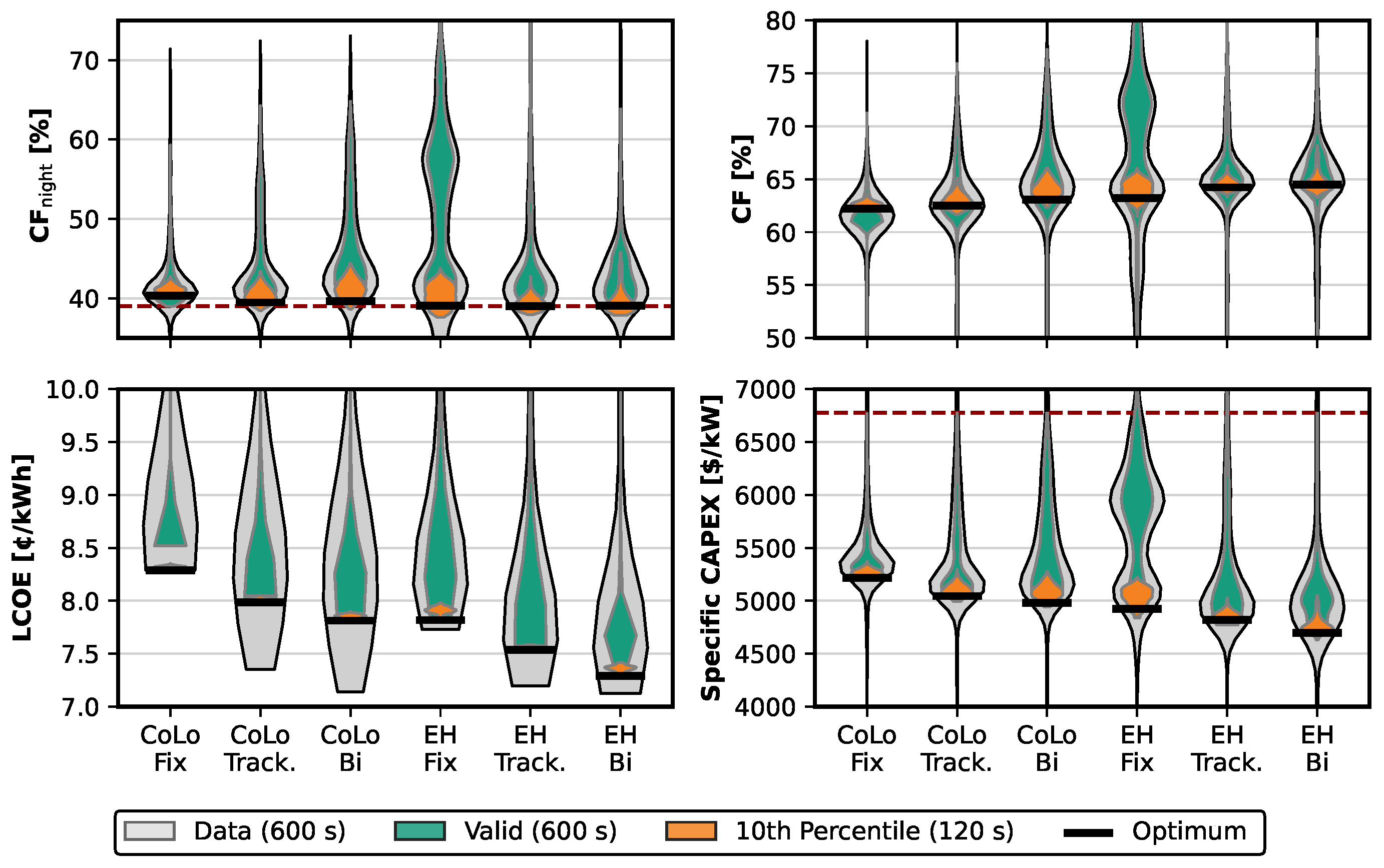
Figure 7 summarizes the optimization outcomes for each configuration. Across all six cases, the optimization converges toward solutions that satisfy the nighttime-capacity-factor requirement while remaining below the specific-CAPEX ceiling. Most 600 s candidates cluster close to the minimum ${\mathrm{CF}}_{\mathrm{night}}$ threshold of 39%, indicating that the optimum generally avoids adding nighttime-delivery capability beyond what is required to minimize LCOE.

While ${\mathrm{CF}}_{\mathrm{night}}$ remains close to this lower bound, the overall capacity factor tends to increase for EH-integrated layouts. This is mainly due to steadier daytime production enabled by larger PV fields, higher $R_{\mathrm{DC}/\mathrm{AC}}$, improved thermal–electric conversion efficiency, and lower relative parasitic losses. The CF values of the optimum configurations are nevertheless relatively close: $62.3–63.2\%$ for the co-located layouts and $63.2–64.5\%$ for the EH-integrated layouts. For the bifacial cases, the EH-integrated configuration attains a $+1.3$ percentage-point-higher CF than the corresponding co-located design. Overall, both hybridization concepts satisfy the performance constraints within the imposed economic bounds.

Despite the large installed capacities, curtailed generation remains below 0.1% for all optimum configurations. For the EH-integrated systems, EH utilization reaches 26.7% for fixed-tilt PV, 28.5% for single-axis tracking PV, and 31.4% for bifacial PV. The LCOE results show a consistent advantage for the EH-integrated layouts. Because these systems deploy nearly twice the PV capacity of the co-located designs, bifacial modules provide a larger benefit by increasing annual energy yield at comparable module cost. Comparing optimum hybrids with the same PV technology, the EH-integrated layout reduces LCOE by approximately $5.6\%$ for fixed-tilt and single-axis PV, and by approximately $6.7\%$ for bifacial PV, relative to the corresponding co-located layouts.

The specific-CAPEX results likewise remain well below the imposed ceiling of $6776/kW. For the optimum designs, specific CAPEX is $22.8–30.6\%$ below this limit. Across both hybridization concepts, PV technology materially affects system cost: replacing fixed-tilt PV with bifacial modules reduces total CAPEX by 4.6% for EH-integrated systems and by 4.5% for co-located systems.

A key outcome of the workflow is that the broad 600 s search, combined with selective 120 s re-simulation of the best-performing candidates and their nearby neighbors, is required to robustly identify the final optimum.

Table 7. Comparison of 600 s and 120 s resolution optima—co-located configurations.

		Fixed		Tracking		Bifacial
	Unit	600 s	120 s	600 s	120 s	600 s	120 s
${\mathrm{Rank}}_{600\mathrm{s}}$	–	#1	#9	#1	#2	#1	#102
${\mathrm{Rank}}_{120\mathrm{s}}$	–	#3	#1	#3	#1	#2	#1
${\mathrm{CF}}_{\mathrm{night},600\mathrm{s}}$	%	39.0	39.1	40.8	39.9	40.7	39.7
${\mathrm{CF}}_{\mathrm{night},120\mathrm{s}}$	%	40.2	40.3	40.4	39.5	40.3	39.6
		+2.9%	+3.1%	−1.1%	−1.1%	−1.0%	−0.2%
${\mathrm{CF}}_{600\mathrm{s}}$	%	60.5	60.5	62.8	62.0	63.0	62.4
${\mathrm{CF}}_{120\mathrm{s}}$	%	62.1	62.2	63.3	62.5	63.5	63.1
		+2.7%	+2.8%	+0.8%	+0.8%	+0.9%	+1.1%
${\mathrm{LCOE}}_{600\mathrm{s}}$	¢/kWh	8.52	8.52	8.05	8.05	7.88	7.90
${\mathrm{LCOE}}_{120\mathrm{s}}$	¢/kWh	8.29	8.29	7.99	7.99	7.82	7.81
		−2.7%	−2.8%	−0.8%	−0.8%	−0.8%	−1.1%
SF loops	–	320 → 322		294		294 → 280
TES capacity	MWhth	4640		4170 → 4111		4111 → 4287
DC/AC ratio	–	2.22		2.14 → 2.06		1.98 → 1.96
Inverter capacity	MWAC	200		200		200
PV tilt angle	°	24.5 → 27.0		–		–
BESS size	MWh	500		500		500 → 475

Note: Italicized percentage values indicate the percent relative change with respect to the baseline case. Arrows (→) indicate the shift from the 600 s optimum value to the 120 s optimum value for the same configuration; a single entry indicates no change between resolutions.

and

Table 8. Comparison of 600 s and 120 s resolution optima—EH-integrated configurations.

		Fixed		Tracking		Bifacial
	Unit	600 s	120 s	600 s	120 s	600 s	120 s
${\mathrm{Rank}}_{600\mathrm{s}}$	–	#1	#122	#1	#39	#1	#5
${\mathrm{Rank}}_{120\mathrm{s}}$	–	Invalid	#1	Invalid	#1	Invalid	#1
${\mathrm{CF}}_{\mathrm{night},600\mathrm{s}}$	%	39.0	40.4	39.2	40.0	39.9	40.2
${\mathrm{CF}}_{\mathrm{night},120\mathrm{s}}$	%	37.7	39.1	38.1	39.0	38.7	39.1
		−3.5%	−3.3%	−2.8%	−2.5%	−2.9%	−2.9%
${\mathrm{CF}}_{600\mathrm{s}}$	%	62.4	63.1	63.7	64.1	64.2	64.4
${\mathrm{CF}}_{120\mathrm{s}}$	%	62.5	63.2	63.8	64.2	64.3	64.5
		+0.1%	+0.2%	+0.1%	+0.2%	+0.2%	+0.1%
${\mathrm{LCOE}}_{600\mathrm{s}}$	¢/kWh	7.80	7.83	7.54	7.55	7.27	7.28
${\mathrm{LCOE}}_{120\mathrm{s}}$	¢/kWh	7.81	7.82	7.53	7.54	7.28	7.29
		+0.2%	−0.2%	−0.1%	−0.2%	+0.1%	+0.1%
SF loops	–	106 → 110		108 → 116		96
TES capacity	MWhth	3438 → 3490		4272 → 4376		3594 → 3751
DC/AC ratio	–	1.76		1.54 → 1.50		1.54
Inverter capacity	MWAC	390 → 395		405 → 420		375
PV tilt angle	°	24.0 → 24.5		–		–
BESS size	MWh	475 → 500		200 → 150		425
EH capacity	MW	190 → 195		205 → 220		175

Note: Italicized percentage values indicate the percent relative change with respect to the baseline case. Arrows (→) indicate the shift from the 600 s optimum value to the 120 s optimum value for the same configuration; a single entry indicates no change between resolutions.

therefore do more than compare two resolutions: they show how temporal refinement changes candidate feasibility, ranking, and final component sizing.

For the co-located configurations, the shift from 600 s to 120 s increases the median annual CF of the re-simulated candidates by 2.9% for fixed-tilt PV and by 0.9% for both tracking and bifacial PV. At the same time, the median ${\mathrm{CF}}_{\mathrm{night}}$ increases by 3.1% for fixed-tilt PV but decreases by 0.8% and 0.6% for the tracking and bifacial cases, respectively. Because these CF and ${\mathrm{CF}}_{\mathrm{night}}$ changes partially offset one another, fewer than 6% of the approximately 1900 re-simulated co-located candidates are invalidated at 120 s.

At higher temporal resolution, neighboring designs to the original 600 s optima often outperform the original best candidate and achieve a lower LCOE. For example, in the fixed-tilt co-located case, the 600 s optimum drops to rank #3 after 120 s re-simulation, while the candidate ranked #9 at 600 s becomes the new optimum. Relative to the original 600 s optimum, the final 120 s design uses a slightly larger solar field and a higher PV tilt angle, which in turn yields slightly higher CF and ${\mathrm{CF}}_{\mathrm{night}}$. A similar effect is observed for the bifacial co-located case, where the final 120 s optimum was ranked only #102 at 600 s. Compared with the original 600 s optimum, this 120 s bifacial design requires fewer solar-field loops, less PV, and a smaller BESS, while slightly increasing TES capacity. In other words, temporal refinement does not merely affect the KPI values; it can change which configuration is judged to be the economically preferred design.

By contrast, the EH-integrated configurations show only a slight increase in annual yield at higher temporal resolution, on the order of 0.1–0.2%, but a more pronounced decrease in ${\mathrm{CF}}_{\mathrm{night}}$ of 2.4–3.2%. This indicates that the coarser 600 s resolution captures annual energy yield reasonably well, but can overestimate nighttime-delivery performance in the more PV-dominant EH-integrated layouts. In particular, the lower temporal resolution smooths short transition periods between daytime PV-driven charging and evening or nighttime TES discharge. Accordingly, compliance with the 39% nighttime-capacity-factor threshold is slightly overestimated. As a result, 20.0–38.8% of the re-simulated candidates are invalidated because they no longer satisfy the ${\mathrm{CF}}_{\mathrm{night}}$ requirement at 120 s.

Consequently, the original 600 s optima for all three EH-integrated configurations are invalidated, and nearby candidates take their place as the final 120 s optima (Table 8). To recover the lost nighttime-delivery margin, the fixed-tilt and tracking EH-integrated configurations increase the size of most major subsystems. The bifacial EH-integrated configuration, however, requires only a modest increase in TES capacity. Despite these shifts in component composition, the resulting LCOE changes remain small, within approximately $\pm 0.2\%$ relative to the 600 s estimate.

Taken together, these two tables highlight the value of the two-stage optimization framework. The broad lower-resolution search efficiently identifies promising regions in the design space, while selective high-resolution re-simulation determines whether apparently optimal candidates remain feasible and competitive once temporal fidelity is increased. For the co-located systems, this process reveals opportunities to reduce cost by removing excess performance margin. For the EH-integrated systems, it shows where slightly larger subsystem capacities are needed to preserve compliance with the nighttime-delivery requirement. More broadly, the comparison shows that temporal resolution does not merely affect the numerical value of individual KPIs; it can also influence whether critical transition periods are represented accurately enough for constraint-based design selection. The key point is therefore not that parameter sizing is arbitrary, but that the final optimum is locally resolution-sensitive even though the broader design trends remain stable.

Across hybridization concepts, the optimized designs also exhibit consistent technology trends, most notably a TES–BESS tradeoff. Many optima favor the maximum BESS capacity of 500 MWh; when a smaller BESS is selected, TES capacity is typically increased to preserve nighttime delivery. This pattern is particularly evident for the EH-integrated layout with single-axis tracking PV, which adopts slightly larger TES together with a somewhat smaller PV + BESS combination. More broadly, these results show that several nearby component combinations can achieve similar techno-economic performance. Thus, parameter sizing matters for final ranking and feasibility, but not every parameter is pinned to a single unique value. Within the imposed constraints, both hybridization concepts remain competitive; however, the EH-integrated configurations consistently achieve lower LCOE and lower CAPEX than the co-located layouts.

5.2. Tradeoff Between Nighttime Delivery and LCOE

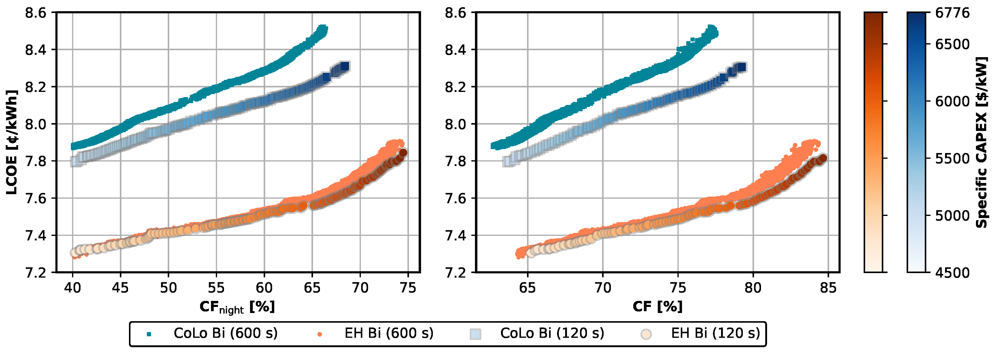
Both hybridization concepts yield feasible designs with ${\mathrm{CF}}_{\mathrm{night}}$ above the minimum constraint at competitive cost (Figure 7). To quantify the cost of higher nighttime delivery under the specific-CAPEX ceiling of $6776/kW, the bifacial co-located and EH-integrated cases are re-optimized while incrementally increasing the ${\mathrm{CF}}_{\mathrm{night}}$ requirement up to 75% in order to form a Pareto front. Points along this front, together with their nearby neighbors, are then re-simulated at 120 s to confirm performance at higher resolution. The resulting Pareto fronts for both configurations and both temporal resolutions are shown in Figure 8.

For both layouts, the Pareto-front behavior is similar in overall shape: LCOE increases as ${\mathrm{CF}}_{\mathrm{night}}$ (Figure 8, left) and CF (Figure 8, right) increase. However, the EH-integrated configurations achieve lower LCOE and higher CF/${\mathrm{CF}}_{\mathrm{night}}$ values than the co-located configurations across the explored range. The 120 s Pareto front of the co-located system extends to nearly 70% ${\mathrm{CF}}_{\mathrm{night}}$ before reaching the specific-CAPEX ceiling.

The mechanism by which ${\mathrm{CF}}_{\mathrm{night}}$ is increased differs between the two hybridization concepts. In the co-located layout, higher nighttime delivery is obtained primarily by increasing PTC capacity in order to charge TES. In the EH-integrated layout, nighttime delivery is increased by adding both PTC capacity and EH capacity, which in turn requires more PV generation to supply the additional electrical input. For the co-located system, additional PTC capacity does not directly improve daytime export because PV already dominates daytime supply. In contrast, in the EH-integrated layout, the added PV + EH combination supports both TES charging and daytime coverage of the 200 MW_el export requirement.

Re-simulation at 120 s improves ${\mathrm{CF}}_{\mathrm{night}}$ for the co-located Pareto-front points, highlighting the stronger time-resolution sensitivity of CSP-dominant nighttime operation. For example, at ${\mathrm{CF}}_{\mathrm{night}}=50\%$, a 600 s co-located solution exhibits a 0.6% increase in nighttime generation at 120 s together with a 1.3% reduction in LCOE. At ${\mathrm{CF}}_{\mathrm{night}}=65\%$, these gains increase to 3.6% and 1.9%, respectively. By contrast, the EH-integrated cases show smaller changes, consistent with the fact that their nighttime performance is less strongly driven by CSP-dominant dispatch alone.

Operationally, increasing ${\mathrm{CF}}_{\mathrm{night}}$ shifts the system away from PV-dominant daytime operation and toward longer periods of storage discharge and sustained thermal operation during the evening and night. The shape of the Pareto front therefore reflects the rising cost of nighttime generation, which requires larger TES, greater thermal input capacity, and/or more daytime surplus electricity available for conversion and storage.

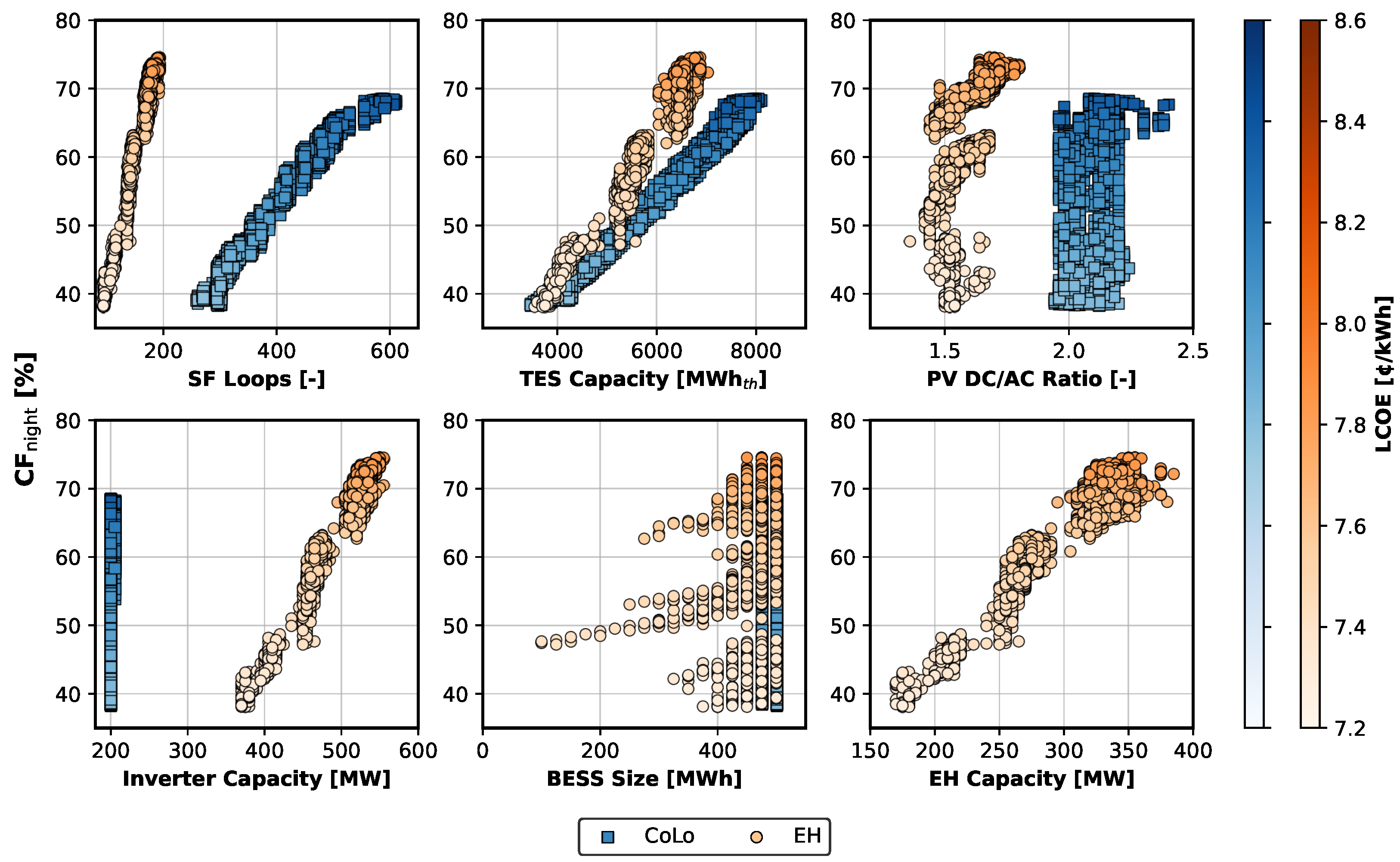
Figure 9 maps the parameter values associated with the 120 s Pareto-front solutions and therefore complements the preceding time-sensitivity analysis. The figure should not be interpreted as implying that parameter sizing is unimportant. Rather, it shows that the main sizing trends are robust, even though several nearby combinations remain competitive within a narrow performance band.

Several parameters exhibit clear trends. For example, the number of solar-field loops increases approximately linearly with ${\mathrm{CF}}_{\mathrm{night}}$ for both concepts, while the EH-integrated configurations form a narrower band than the co-located configurations. In the EH-integrated concept, the required solar-field size is more tightly constrained by the EH coupling between the lower and upper cycles for a given nighttime-delivery target. The co-located concept allows a broader range of loop counts that still yields similar outcomes.

TES capacity also increases with ${\mathrm{CF}}_{\mathrm{night}}$ for both concepts, but the EH-integrated layouts generally require less TES for comparable nighttime performance. This is consistent with the role of the EH-assisted topping cycle and the higher thermal–electric conversion efficiency of the integrated power block. By contrast, the PV DC/AC ratio forms a near-vertical cluster for each concept, indicating that a preferred ratio is selected largely independently of the exact ${\mathrm{CF}}_{\mathrm{night}}$ target. The difference between these preferred values—approximately 2.2 for the co-located layout and 1.5 for the EH-integrated layout—reflects the distinct role of PV in the two concepts.

The BESS results show a strong preference for the largest allowed capacities, with many Pareto-front solutions clustering above 400 MWh. This suggests that the optimized configurations generally benefit from larger battery capacities and that extending the BESS search range could be worthwhile in future optimization runs. By contrast, EH capacity exhibits a broader range at higher ${\mathrm{CF}}_{\mathrm{night}}$. For example, near ${\mathrm{CF}}_{\mathrm{night}}=70\%$, the EH capacity spans approximately 300–350 MW while still yielding competitive techno-economic outcomes.

Taken together, these parameter-sizing trends show that the optimized solutions are not defined by a single fixed composition. Some parameters are consistently pushed toward clear bounds, whereas others retain greater local flexibility while still satisfying the imposed performance criteria. A key benefit of the presented optimization approach is therefore not only the identification of one optimum, but also the generation of multiple solutions that support robust design selection by showing which sizing adjustments remain techno-economically competitive.

Beyond comparing configurations, these Pareto fronts also function as a planning tool: they translate a nighttime-delivery requirement into an explicit LCOE premium and associated component sizing. This is particularly relevant for tenders and grid-planning contexts in which dispatchability is valued but not directly priced. The slope of the front can therefore be interpreted as the incremental cost of additional nighttime supply, enabling a like-for-like comparison of design choices such as larger TES versus larger PV together with EH/BESS under a common economic bound.

5.3. Component Price Sensitivity Along the Pareto Front

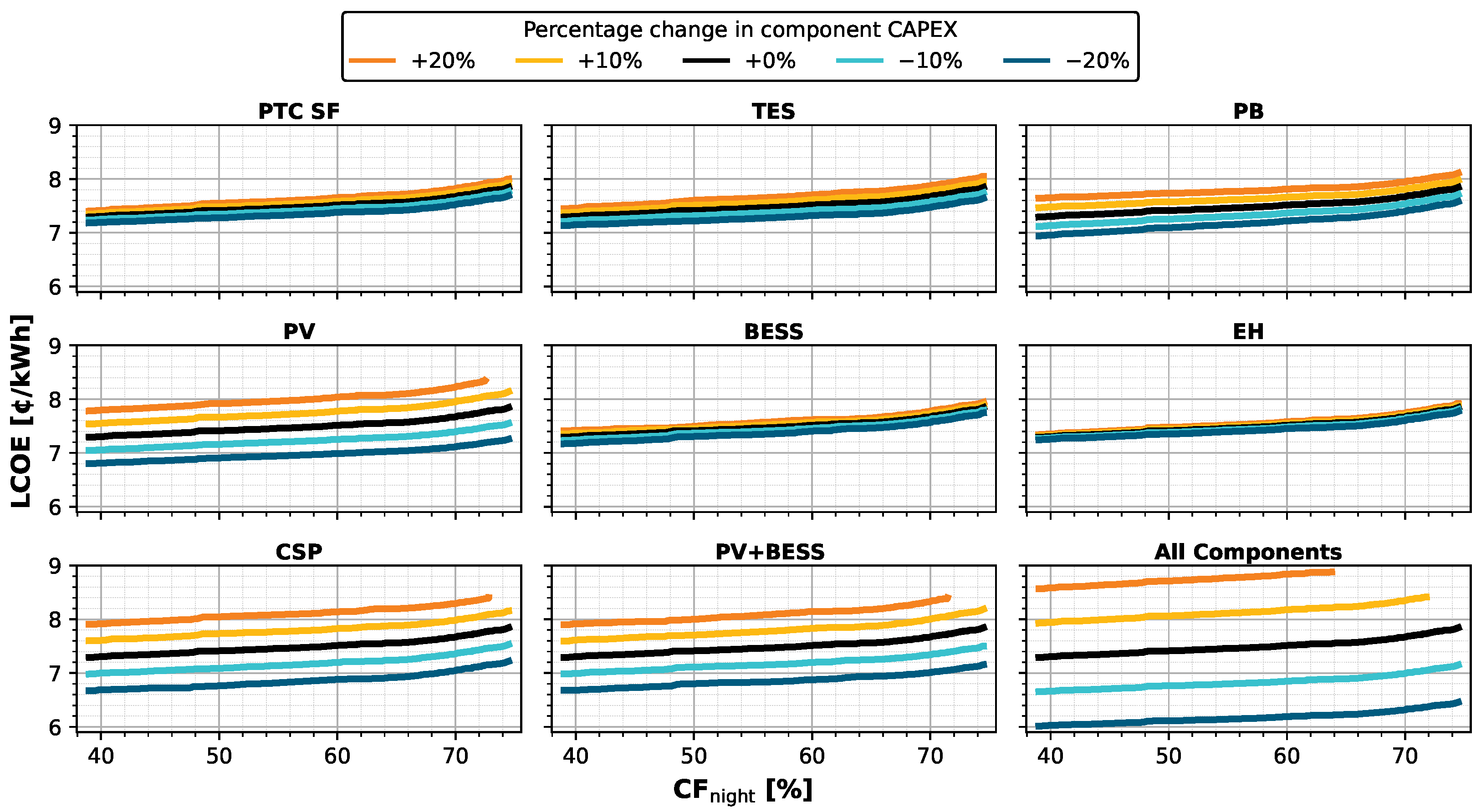
The high-resolution (120 s) Pareto-front results for the EH-integrated bifacial PV configuration are used to assess price sensitivity. Component prices—individually, in combinations, and collectively—are shifted by $\pm 10\%$ and $\pm 20\%$ to reflect both cost-reduction trends [9] and inflationary pressures [51]. For each scenario, CAPEX and LCOE are recomputed, and the configuration with the lowest LCOE is selected (Figure 10).

The impact of CAPEX changes varies by component and by the required ${\mathrm{CF}}_{\mathrm{night}}$ level (

Table 9. Summary of relative LCOE changes for selected component CAPEX variations at different ${\mathrm{CF}}_{\mathrm{night}}$ targets. Positive values indicate higher LCOE than the reference case, while negative values indicate lower LCOE.

	${\mathbf{CF}}_{\mathbf{night}}=39\%$			${\mathbf{CF}}_{\mathbf{night}}=50\%$			${\mathbf{CF}}_{\mathbf{night}}=70\%$
CAPEX Change	$+\mathbf{10}\%$	−10%	−20%	$+\mathbf{10}\%$	−10%	−20%	$+\mathbf{10}\%$	−10%	−20%
Reference LCOE	7.29 ¢/kWh			7.41 ¢/kWh			7.68 ¢/kWh
PTC SF	+0.8%	−0.8%	−1.5%	+0.9%	−0.9%	−1.8%	+1.0%	−1.0%	−1.9%
TES	+1.1%	−1.1%	−2.2%	+1.3%	−1.3%	−2.6%	+1.3%	−1.3%	−2.6%
PB	+2.4%	−2.4%	−4.8%	+2.2%	−2.2%	−4.3%	+1.8%	−1.8%	−3.6%
PV	+3.4%	−3.4%	−6.7%	+3.4%	−3.4%	−6.8%	+3.6%	−3.6%	−7.3%
BESS	+0.8%	−0.8%	−1.7%	+0.5%	−0.7%	−1.5%	+0.7%	−0.7%	−1.3%
EH	+0.3%	−0.3%	−0.7%	+0.4%	−0.4%	−0.9%	+0.5%	−0.5%	−0.9%
CSP	+4.2%	−4.2%	−8.5%	+4.3%	−4.4%	−8.8%	+4.1%	−4.1%	−8.1%
PV+BESS	+4.2%	−4.2%	−8.4%	+4.0%	−4.1%	−8.3%	+4.3%	−4.3%	−8.6%
All Components	+8.8%	−8.8%	−17.5%	+8.8%	−8.8%	−17.6%	+8.8%	−8.8%	−17.7%

). For the individual CSP subsystems, a 20% cost reduction lowers LCOE by 1.5–4.8% at ${\mathrm{CF}}_{\mathrm{night}}=39\%$, 1.8–4.3% at ${\mathrm{CF}}_{\mathrm{night}}=50\%$, and 1.9–3.6% at ${\mathrm{CF}}_{\mathrm{night}}=70\%$, with the power block showing the strongest individual effect. By contrast, the effect of EH and BESS price reductions is smaller: a 20% CAPEX reduction lowers LCOE by only 0.7–0.9% for EH and 1.3–1.7% for BESS across the three nighttime-delivery targets. PV cost reductions are more influential, which is consistent with the large PV share in the optimized systems: a 20% PV-CAPEX reduction lowers LCOE by approximately 6.7–7.3%, depending on the ${\mathrm{CF}}_{\mathrm{night}}$ requirement.

Overall, PV and power-block costs emerge as the most influential individual drivers of LCOE, whereas EH has a comparatively minor effect. In aggregate, PV + BESS or CSP-component cost reductions produce similar combined impacts of roughly $\pm 8.0\%$ to $\pm 8.8\%$, depending on the ${\mathrm{CF}}_{\mathrm{night}}$ target. If all component costs decrease by 10–20%, an LCOE below 7 ¢/kWh becomes achievable even for configurations with ${\mathrm{CF}}_{\mathrm{night}}>70\%$.

Changes in component prices can also shift the optimum within the design space. For example, under a ${\mathrm{CF}}_{\mathrm{night}}=50\%$ requirement and a 20% reduction in PV + BESS prices, the EH-integrated optimum moves toward a more electrically dominated storage configuration: $R_{\mathrm{DC}/\mathrm{AC}}$ increases from 1.44 to 1.50; inverter capacity decreases from 455 to $435{\mathrm{MW}}_{\mathrm{AC}}$; EH capacity decreases from 255 to $240\mathrm{MW}$; TES decreases from $10.1$ to $9.1\mathrm{FLH}$; PTC loops decrease from 136 to 124; and BESS increases from 250 to $450\mathrm{MWh}$. This again illustrates the practical value of a large-candidate optimization: when financial assumptions change, nearby candidate solutions provide credible guidance on how the optimum migrates through the design space.

Given the market-driven uncertainty in installed costs, these sensitivities help to contextualize the robustness of the optimal design choices. The results indicate that the objective is most sensitive to PV and power-block CAPEX, whereas TES, EH, and BESS costs exert smaller marginal effects over the tested range. At the same time, the observed parameter shifts under price adjustments show that the design space contains multiple near-optimal solutions, suggesting that moderate cost revisions are more likely to move the optimum locally than to overturn the relative ranking of the configurations.

6. Conclusions

Large-scale solar developments in Morocco—including the Noor Ouarzazate complex and the planned Noor Midelt project—highlight the need for renewable-energy plants that combine low-cost generation with dispatchability.

This study developed and applied a high-resolution simulation and techno-economic optimization framework to quantify the design space of CSP–PV hybrid plants in Midelt. The framework operates under tender-style constraints: a fixed power purchase agreement (PPA), a $200{\mathrm{MW}}_{\mathrm{el}}$ export limit, a CAPEX ceiling, and a nighttime-delivery requirement expressed as a minimum nighttime capacity factor.

Two hybridization concepts were evaluated. The first is a co-located CSP–PV plant in which PV and CSP interact at the grid level, with PV primarily supporting daytime export and BESS charging, while CSP supplies nighttime export. The second is an EH-integrated plant in which surplus PV electricity is converted to heat via an electric heater (EH) and stored in molten-salt TES. A surrogate-assisted genetic algorithm explored more than 200,000 candidate designs at 600 s temporal resolution and re-simulated the top candidates at 120 s to reduce discretization error and improve final design selection.

Across the evaluated configurations, EH integration and bifacial PV emerged as the most favorable combination under the adopted constraints. The lowest-LCOE solution is the EH-integrated bifacial configuration (120 s optimum), achieving an LCOE of $7.29¢/\mathrm{kWh}$ at a specific CAPEX of $4698/kW, with less than 0.1% curtailment, an overall capacity factor of 64.5%, and ${\mathrm{CF}}_{\mathrm{night}}=39.1\%$. The best co-located bifacial configuration achieves $7.81¢/\mathrm{kWh}$, confirming that technology-level hybridization via EH can lower LCOE while increasing overall capacity factor under a constant-power export constraint.

The results also show that temporal resolution is not merely a numerical detail, but can influence both feasibility assessment and final design selection. For the co-located configurations, re-simulation at 120 s shifts annual CF, LCOE, and candidate ranking sufficiently that nearby configurations can replace the original 600 s optimum. For the EH-integrated configurations, annual yield and LCOE change only slightly with temporal refinement. However, ${\mathrm{CF}}_{\mathrm{night}}$ decreases more because the coarser 600 s resolution smooths the short transition periods between daytime PV-driven charging and evening TES discharge. As a result, several candidates that appear feasible at 600 s become invalid at 120 s. The adopted two-stage workflow therefore serves not only to reduce computational cost, but also to improve the robustness of constraint-based design selection.

Pareto fronts constructed by progressively increasing the nighttime-delivery target quantify the cost of higher ${\mathrm{CF}}_{\mathrm{night}}$ under the imposed CAPEX ceiling. These fronts show that LCOE increases as nighttime delivery is tightened, while the EH-integrated configurations remain consistently more favorable than the co-located ones across the explored range. The two hybridization concepts achieve higher nighttime delivery through different mechanisms: the co-located concept relies primarily on additional PTC capacity and TES charging, whereas the EH-integrated concept combines added PTC capacity with EH and PV expansion. The Pareto fronts therefore provide not only a cost–performance tradeoff, but also a practical sizing guide for how the dominant design levers shift as nighttime-delivery requirements become more stringent.

The parameter trends along the Pareto fronts further show that the optimized systems are not defined by a single fixed composition. Some parameters are consistently pushed toward clear bounds, whereas others retain greater local flexibility while still satisfying the imposed performance criteria. In this sense, a key benefit of the presented optimization framework is not only the identification of one optimum, but also the generation of neighboring candidates that support robust design selection and clarify which sizing adjustments remain techno-economically competitive.

The presented results depend on the adopted cost assumptions, and actual EPC costs can vary substantially. Nonetheless, the price-sensitivity analysis shows that PV and power-block costs are the most influential individual drivers of LCOE, while TES, EH, and BESS costs exert smaller marginal effects over the tested range. At the same time, the observed parameter shifts under price adjustments show that moderate cost revisions are more likely to move the optimum locally within the design space than to overturn the relative ranking of the configurations.

A distinguishing contribution of this work lies in the two-stage optimization workflow, in which broad screening at 600 s is followed by the selective re-simulation of leading candidates at 120 s. Within the Midelt design case, this workflow allows co-located and EH-integrated concepts to be compared under the same constraints while accounting for multiple PV technologies, localized cost assumptions, and coupled component-sizing decisions. The results show that temporal resolution affects not only reported KPI values, but also candidate feasibility, final sizing, and preferred design selection. The Pareto-front and parameter-trend analyses extend the interpretation beyond a single optimum by showing how nighttime-delivery requirements reshape both the cost tradeoff and the neighborhood of near-optimal solutions.

The results should be interpreted in light of several limitations. First, the hybridization analysis relies on representative weather data. In particular, using several consecutive years of measured data from a local weather station would introduce inter-annual variability that could shift the resulting optimal configurations. Second, the cost assumptions aim to reflect localized values. However, actual EPC costs, particularly for BESS, vary with market conditions, supply-chain effects, project scale, and technology choice. Finally, some component models adopt simplified performance assumptions. Including detailed representations, such as part-load efficiency curves for the EH and BESS cycling-degradation effects, could influence the simulated performance and relative ranking of the hybrid plant configurations.

Building on these results, future work could explore (i) alternative market formulations, including time-varying prices, ancillary services, and peak-delivery requirements; (ii) additional operational realism, such as start-up and ramp limits, minimum-load constraints, mirror-cleaning schedules, and more detailed thermal-loss modeling; (iii) expanded uncertainty quantification for component costs, degradation, and financing; and (iv) multi-site studies using locally measured meteorological data.

Overall, the results show that well-designed CSP–PV hybrids can satisfy grid-oriented performance constraints while combining low-cost PV with dispatchable TES. More broadly, these findings suggest that current and future standalone renewable-energy projects can benefit from hybridization and sector coupling, including power-to-heat-to-X pathways, for both electricity and process-heat applications, particularly in systems that aim to combine high capacity factors with dispatchable operation. For project developers and tendering bodies, the presented methodology offers a practical basis for comparing hybridization concepts, defining techno-economic preferences, and screening future project configurations under dispatch-oriented procurement frameworks.

References

1. International Renewable Energy Agency. Renewable Energy Statistics 2024; IRENA: Masdar City, United Arab Emirates, 2024.
2. Platzer, W. PV–Enhanced Solar Thermal Power. Energy Procedia 2014, 57, 477–486. [Google Scholar] [CrossRef]
3. National Renewable Energy Laboratory (NREL). Concentrating Solar Power Projects (SolarPACES Database). Available online: https://solarpaces.nrel.gov/ (accessed on 5 March 2025).
4. African Development Bank. Noor Midelt Solar Complex Project—Phase I (NoorMI and NoorMII Solar Plants); Project Appraisal Report RDGN/PERN; African Development Bank: Abidjan, Côte d’Ivoire, 2017. [Google Scholar]
5. Reuters Staff. Moroccan Solar Plans Hampered by Dispute Over Technology. 2024. Available online: https://www.reuters.com/world/africa/moroccan-solar-plans-hampered-by-dispute-over-technology-2024-02-27/ (accessed on 5 March 2025).
6. Zhang, H.; Baeyens, J.; Degrève, J.; Cacères, G. Concentrated solar power plants: Review and design methodology. Renew. Sustain. Energy Rev. 2013, 22, 466–481. [Google Scholar] [CrossRef]
7. Thonig, R.; Gilmanova, A.; Lilliestam, J. CSP.guru 2023-07-01; Zenodo: Geneva, Switzerland, 2023. [Google Scholar] [CrossRef]
8. Fuqiang, W.; Ziming, C.; Jianyu, T.; Yuan, Y.; Yong, S.; Linhua, L. Progress in concentrated solar power technology with parabolic trough collector system: A comprehensive review. Renew. Sustain. Energy Rev. 2017, 79, 1314–1328. [Google Scholar] [CrossRef]
9. International Renewable Energy Agency. Renewable Power Generation Costs in 2023; IRENA: Masdar City, United Arab Emirates, 2024.
10. Cole, W.; Karmakar, A. Cost Projections for Utility-Scale Battery Storage: 2023 Update; Technical Report NREL/TP–6A40-85332; National Renewable Energy Laboratory (NREL): Golden, CO, USA, 2023. [Google Scholar] [CrossRef]
11. Hesse, H.; Schimpe, M.; Kucevic, D.; Jossen, A. Lithium-Ion Battery Storage for the Grid—A Review of Stationary Battery Storage System Design Tailored for Applications in Modern Power Grids. Energies 2017, 10, 2107. [Google Scholar] [CrossRef]
12. Ramasamy, V.; Zuboy, J.; Woodhouse, M.; O’Shaughnessy, E.; Feldman, D.; Desai, J.; Walker, A.; Margolis, R.; Basore, P. U.S. Solar Photovoltaic System and Energy Storage Cost Benchmarks, with Minimum Sustainable Price Analysis: Q1 2023; Technical Report NREL/TP-7A40-87303; National Renewable Energy Laboratory (NREL): Golden, CO, USA, 2023. [Google Scholar] [CrossRef]
13. Green, A.; Diep, C.; Dunn, R.; Dent, J. High Capacity Factor CSP-PV Hybrid Systems. Energy Procedia 2015, 69, 2049–2059. [Google Scholar] [CrossRef]
14. Starke, A.; Cardemil, J.; Escobar, R.; Colle, S. Assessing the performance of hybrid CSP+PV plants in northern Chile. Sol. Energy 2016, 138, 88–97. [Google Scholar] [CrossRef]
15. Starke, A.; Cardemil, J.; Escobar, R.; Colle, S. Multi-objective optimization of hybrid CSP+PV system using genetic algorithm. Energy 2018, 147, 490–503. [Google Scholar] [CrossRef]
16. Bousselamti, L.; Ahouar, W.; Cherkaoui, M. Multi-objective optimization of PV-CSP system in different dispatch strategies, case of study: Midelt city. J. Renew. Sustain. Energy 2021, 13. [Google Scholar] [CrossRef]
17. Benitez, D.; Röger, M.; Kazantzidis, A.; Al-Salaymeh, A.; Bouaichaoui, S.; Guizani, A.; Balghouthi, M. Hybrid CSP—PV Plants for Jordan, Tunisia and Algeria. Energies 2023, 16, 924. [Google Scholar] [CrossRef]
18. Bode, S.; Cuellar, A.; Perez, I. Retrofitting operating CSP plants with PV to power auxiliary loads – Technical consideration and case study. In Proceedings of the 24th SolarPACES Conference, Casablanca, Morocco, 2–5 October 2018; AIP Publishing: Melville, NY, USA, 2019; Volume 2126, p. 90003. [Google Scholar] [CrossRef]
19. Gedle, Y.; Schmitz, M.; Schmitz, P.; Herrmann, U.; Boura, C.; Mahdi, Z.; Caminos, R.C.; Merige, P.; Dersch, J. Analysis of an Integrated CSP-PV hybrid power plant. In Proceedings of the 26th SolarPACES Conference, Online, 28 September–2 October 2021; AIP Publishing: Melville, NY, USA, 2022; Volume 2445, p. 030009. [Google Scholar] [CrossRef]
20. Iñigo-Labairu, J.; Dersch, J.; Schomaker, L. Integration of CSP and PV Power Plants: Investigations about Synergies by Close Coupling. Energies 2022, 15, 7103. [Google Scholar] [CrossRef]
21. Guccione, S.; Guedez, R. Techno-economic optimization of molten salt based CSP plants through integration of supercritical CO2 cycles and hybridization with PV and electric heaters. Energy 2023, 283, 128528. [Google Scholar] [CrossRef]
22. Mahdi, Z.; Herrmann, U.; Görner, K. Operation Optimization of a Power-to-Heat System in PV-CSP Hybrid Power Plants Together with Molten Salt Thermal Storage. In Proceedings of the International Renewable Energy Storage and Systems Conference (IRES 2023), Aachen, Germany, 28–30 November 2023; Atlantis Press: Dordrecht, The Netherlands, 2024; Volume 328, pp. 212–218. [Google Scholar] [CrossRef]
23. Giuliano, S.; Puppe, M.; Noureldin, K. Power-to-heat in CSP systems for capacity expansion. In Proceedings of the 24th SolarPACES Conference, Casablanca, Morocco, 2–5 October 2018; AIP Publishing: Melville, NY, USA, 2019; Volume 2126, p. 60003. [Google Scholar] [CrossRef]
24. Pilotti, L.; Colombari, M.; Castelli, A.; Binotti, M.; Giaconia, A.; Martelli, E. Simultaneous design and operational optimization of hybrid CSP-PV plants. Appl. Energy 2023, 331, 120369. [Google Scholar] [CrossRef]
25. Guo, S.; He, Y.; Pei, H.; Wu, S. The multi-objective capacity optimization of wind-photovoltaic-thermal energy storage hybrid power system with electric heater. Sol. Energy 2020, 195, 138–149. [Google Scholar] [CrossRef]
26. Petrollese, M.; Cocco, D. Optimal design of a hybrid CSP-PV plant for achieving the full dispatchability of solar energy power plants. Sol. Energy 2016, 137, 477–489. [Google Scholar] [CrossRef]
27. Hassani, S.; Ouali, H.; Moussaoui, M.; Mezrhab, A. Techno-Economic Analysis of a Hybrid CSP/PV Plants in the Eastern Region of Morocco. Appl. Sol. Energy 2021, 57, 297–309. [Google Scholar] [CrossRef]
28. Jbaihi, O.; Ouchani, F.; Merrouni, A.A.; Cherkaoui, M.; Ghennioui, A.; Maaroufi, M. An AHP-GIS based site suitability analysis for integrating large-scale hybrid CSP+PV plants in Morocco: An approach to address the intermittency of solar energy. J. Clean. Prod. 2022, 369, 133250. [Google Scholar] [CrossRef]
29. Zurita, A.; Mata-Torres, C.; Cardemil, J.; Escobar, R. Assessment of time resolution impact on the modeling of a hybrid CSP-PV plant: A case of study in Chile. Sol. Energy 2020, 202, 553–570. [Google Scholar] [CrossRef]
30. Wittwer, C. ColSim—Simulation von Regelungssystemen in Aktiven Solarthermischen Anlagen. Ph.D. Thesis, Karlsruhe Institut für Technologie, Karlsruhe, Germany, 1999. [Google Scholar]
31. Rohani, S.; Fluri, T.; Dinter, F.; Nitz, P. Modelling and simulation of parabolic trough plants based on real operating data. Sol. Energy 2017, 158, 845–860. [Google Scholar] [CrossRef]
32. Gomez Garcia, S.; Rohani, S.; Chandler, N.; Schöttl, P.; Kraft, T.; Bern, G. Maintenance Optimization of Parabolic Trough Power Plants Through a Lifetime Simulation Model Validated with Five-Years of Operational Data. In Proceedings of the 30th SolarPACES Conference; TIB Open Publishing: Rome, Italy, 2025; Volume 3. [Google Scholar] [CrossRef]
33. African Development Bank. Morocco Noor Ouarzazate Solar Complex Project—Phase II (Noor Ouarzazate II Power Plant) Project Completion Report; Project Completion Report; African Development Bank: Abidjan, Côte d’Ivoire, 2020; Public Disclosure Authorized. [Google Scholar]
34. Remund, J.; Müller, S.; Schmutz, M.; Graf, P. Meteonorm Version 8. In Proceedings of the European PVSEC 2020, Online, 7–11 September 2020. [Google Scholar]
35. Gilman, P. SAM Photovoltaic Model Technical Reference; Technical Report NREL/TP-6A20-64102; National Renewable Energy Laboratory (NREL): Golden, CO, USA, 2015. [Google Scholar] [CrossRef]
36. Soto, W.D.; Klein, S.; Beckman, W. Improvement and validation of a model for photovoltaic array performance. Sol. Energy 2006, 80, 78–88. [Google Scholar] [CrossRef]
37. Duffie, J.; Beckman, W. Solar Engineering of Thermal Processes, 4th ed.; John Wiley & Sons, Inc.: Hoboken, NJ, USA, 2013. [Google Scholar] [CrossRef]
38. National Renewable Energy Laboratory (NREL). System Advisor Model (SAM), Version 2025.4.16; NREL: Golden, CO, USA, 2025.
39. Mousazadeh, H.; Keyhani, A.; Javadi, A.; Mobli, H.; Abrinia, K.; Sharifi, A. A review of principle and sun-tracking methods for maximizing solar systems output. Renew. Sustain. Energy Rev. 2009, 13, 1800–1818. [Google Scholar] [CrossRef]
40. Appelbaum, J.; Bany, J. Shadow effect of adjacent solar collectors in large scale systems. Sol. Energy 1979, 23, 497–507. [Google Scholar] [CrossRef]
41. Deline, C.; Dobos, A.; Janzou, S.; Meydbray, J.; Donovan, M. A simplified model of uniform shading in large photovoltaic arrays. Sol. Energy 2013, 96, 274–282. [Google Scholar] [CrossRef]
42. Ajdid, R.; Ouassaid, M.; Maaroufi, M. Power output evaluation of polycrystalline PV panel under various irradiances and temperatures in Moroccan regions. In Proceedings of the 2015 International Conference on Electrical and Information Technologies (ICEIT); IEEE: Marrakech, Morocco, 2015; pp. 257–262. [Google Scholar] [CrossRef]
43. Rodríguez-Gallegos, C.; Bieri, M.; Gandhi, O.; Singh, J.; Reindl, T.; Panda, S. Monofacial vs bifacial Si-based PV modules: Which one is more cost-effective? Sol. Energy 2018, 176, 412–438. [Google Scholar] [CrossRef]
44. VDMA. International Technology Roadmap for Photovoltaics (ITRPV); Technical report; VDMA: Frankfurt am Main, Germany, 2025. [Google Scholar]
45. Holmgren, W.F.; Hansen, C.W.; Mikofski, M.A. pvlib python: A python package for modeling solar energy systems. J. Open Source Softw. 2018, 3, 884. [Google Scholar] [CrossRef]
46. Mikofski, M.; Darawali, R.; Hamer, M.; Neubert, A.; Newmiller, J. Bifacial Performance Modeling in Large Arrays. In Proceedings of the 2019 IEEE 46th Photovoltaic Specialists Conference (PVSC); IEEE: Chicago, IL, USA, 2019; pp. 1282–1287. [Google Scholar] [CrossRef]
47. Zurita, A.; Mata-Torres, C.; Valenzuela, C.; Felbol, C.; Cardemil, J.M.; Guzmán, A.M.; Escobar, R.A. Techno-economic evaluation of a hybrid CSP + PV plant integrated with thermal energy storage and a large-scale battery energy storage system for base generation. Sol. Energy 2018, 173, 1262–1277. [Google Scholar] [CrossRef]
48. Dieckmann, S.; Dersch, J.; Giuliano, S.; Puppe, M.; Lüpfert, E.; Hennecke, K.; Pitz-Paal, R.; Taylor, M.; Ralon, P. LCOE reduction potential of parabolic trough and solar tower CSP technology until 2025. In Proceedings of the 22nd SolarPACES Conference, Abu Dhabi, United Arab Emirates, 11–14 October 2016; AIP Publishing: Melville, NY, USA, 2017; Volume 1850, p. 160004. [Google Scholar] [CrossRef]
49. Hirsch, T.; Bachelier, C.; Eck, M.; Dersch, J.; Fluri, T.; Giuliano, S.; Goebel, O.; González, L.; Haller, U.; Meyer, R.; et al. The first version of the SolarPACES guideline for bankable STE yield assessment. In Proceedings of the 22nd SolarPACES Conference, Abu Dhabi, United Arab Emirates, 11–14 October 2016; AIP Publishing: Melville, NY, USA, 2017; Volume 1850, p. 160014. [Google Scholar] [CrossRef]
50. Dersch, J.; Dieckmann, S.; Hennecke, K.; Pitz-Paal, R.; Taylor, M.; Ralon, P. LCOE reduction potential of parabolic trough and solar tower technology in G20 countries until 2030. In Proceedings of the 25th SolarPACES Conference, Daegu, South Korea, 1–4 October 2019; AIP Publishing: Melville, NY, USA, 2020; Volume 2303, p. 120002. [Google Scholar] [CrossRef]
51. World Bank. Inflation, Consumer Prices (Annual %): Morocco. 2025. Available online: https://data.worldbank.org/indicator/FP.CPI.TOTL.ZG (accessed on 5 March 2025).
52. Augustine, C.; Blair, N. Storage Futures Study: Storage Technology Modeling Input Data Report; Technical Report NREL/TP–5700-78694; National Renewable Energy Laboratory (NREL): Golden, CO, USA, 2021. [Google Scholar] [CrossRef]
53. Li, F.; Li, C.; Sun, K.; Zhang, J.; Li, H. Capacity configuration of hybrid CSP/PV plant for economical application of solar energy. Chin. J. Electr. Eng. 2020, 6, 19–29. [Google Scholar] [CrossRef]
54. Konstantin, P. Praxisbuch Energiewirtschaft; Springer: Berlin/Heidelberg, Germany, 2009. [Google Scholar] [CrossRef]
55. Kost, C.; Mayer, J.; Thomsen, J.; Hartmann, N.; Senkpiel, C.; Philipps, S.; Nold, S.; Lude, S.; Saad, N.; Schlegl, T. Levelized Cost of Electricity-Renewable Energy Technologies; Technical report; Fraunhofer Institute for Solar Energy Systems ISE: Freiburg im Breisgau, Germany, 2013. [Google Scholar]
56. Eiben, A.; Smith, J. Introduction to Evolutionary Computing; Natural Computing Series; Springer: Berlin/Heidelberg, Germany, 2015. [Google Scholar] [CrossRef]
57. Pedregosa, F.; Varoquaux, G.; Gramfort, A.; Michel, V.; Thirion, B.; Grisel, O.; Blondel, M.; Prettenhofer, P.; Weiss, R.; Dubourg, V.; et al. Scikit-learn: Machine learning in Python. J. Mach. Learn. Res. 2011, 12, 2825–2830. [Google Scholar]
58. McKay, M.; Beckman, R.; Conover, W. A comparison of three methods for selecting values of input variables in the analysis of output from a computer code. Technometrics 2000, 42, 55–61. [Google Scholar] [CrossRef]
59. Virtanen, P.; Gommers, R.; Oliphant, T.; Haberland, M.; Reddy, T.; Cournapeau, D.; Burovski, E.; Peterson, P.; Weckesser, W.; Bright, J.; et al. SciPy 1.0: Fundamental algorithms for scientific computing in Python. Nat. Methods 2020, 17, 261–272. [Google Scholar] [CrossRef] [PubMed]
60. Viana, F.; Venter, G.; Balabanov, V. An algorithm for fast optimal Latin hypercube design of experiments. Int. J. Numer. Methods Eng. 2010, 82, 135–156. [Google Scholar] [CrossRef]
61. Turchi, C.; Boyd, M.; Kesseli, D.; Kurup, P.; Mehos, M.; Neises, T.; Sharan, P.; Wagner, M.; Wendelin, T. CSP Systems Analysis—Final Project Report; Technical Report NREL/TP-5500-72856; National Renewable Energy Laboratory (NREL): Golden, CO, USA, 2019. [Google Scholar] [CrossRef]
62. Feldman, D.; Zuboy, J.; Dummit, K.; Stright, D.; Heine, M.; Grossman, S.; Margolis, R. Spring 2024 Solar Industry Update; Technical Report NREL/PR–7A40-90042; National Renewable Energy Laboratory (NREL): Golden, CO, USA, 2024. [Google Scholar] [CrossRef]
63. Rodríguez-Gallegos, C.D.; Liu, H.; Gandhi, O.; Singh, J.P.; Krishnamurthy, V.; Kumar, A.; Stein, J.S.; Wang, S.; Li, L.; Reindl, T.; et al. Global Techno-Economic Performance of Bifacial and Tracking Photovoltaic Systems. Joule 2020, 4, 1514–1541. [Google Scholar] [CrossRef]
64. Ramasamy, V.; Feldman, D.; Desai, J.; Margolis, R. U.S. Solar Photovoltaic System and Energy Storage Cost Benchmarks: Q1 2021; Technical Report NREL/TP-7A40-80694; National Renewable Energy Laboratory (NREL): Golden, CO, USA, 2021. [Google Scholar] [CrossRef]
65. Fu, R.; Feldman, D.; Margolis, R. U.S. Solar Photovoltaic System Cost Benchmark: Q1 2018; Technical Report NREL/TP-6A20-72399; National Renewable Energy Laboratory (NREL): Golden, CO, USA, 2018. [Google Scholar] [CrossRef]
Figure 1. (Left): co-located CSP–PV hybrid plant. (Right): CSP–PV hybrid plant with an electric heater operating as a topping cycle.
Energies 19 02461 g001
Figure 2. Three-day time series for a JA Solar 460 module (single-axis tracking) in Ouarzazate, Morocco: (top) available and absorbed direct/diffuse irradiance; (middle) I mp and V mp ; (bottom) module efficiency, ambient and module temperatures.
Energies 19 02461 g002
Figure 3. Comparison of single-axis tracking angles [°] calculated by SAM and ColSim for four representative days.
Energies 19 02461 g003
Figure 4. Monthly comparison of ColSim and SAM for a 100 MW bifacial PV simulation in Ouarzazate, Morocco, showing AC and DC generation (bars) and the relative differences (right axis).
Energies 19 02461 g004
Figure 5. Representative time-series outputs of the EH-integrated hybrid plant for two spring days: (top) DNI, (second) electrical power flows (PV to grid, PV to EH, CSP gross/net, and BESS), (third) storage levels (hot-tank level and BESS SOC), and (bottom) operating temperatures at key locations (solar-field inlet/outlet, EH outlet, and hot-tank temperature).
Energies 19 02461 g005
Figure 6. Simulation performance for three configurations as the time step is refined from 15 min to 30 s. (Top): total runtime. (Bottom): relative yield difference versus the 30 s baseline.
Energies 19 02461 g006
Figure 7. Optimization outcomes for the six hybrid configurations at 600 s resolution. The violin plots show the distributions of CF night , CF, LCOE, and specific CAPEX for the full candidate set (gray) and the valid subset (green). The orange violins denote the top-decile candidates re-simulated at 120 s, and the black markers indicate the final optima selected after 120 s validation. The dashed red lines indicate the minimum nighttime-capacity-factor requirement of 39% and the specific-CAPEX ceiling of $6776/kW.
Energies 19 02461 g007
Figure 8. Pareto fronts for the bifacial co-located and EH-integrated configurations. The left panel shows LCOE as a function of CF night , and the right panel shows LCOE as a function of overall CF. Small markers represent the 600 s optimization results, whereas the larger markers denote the corresponding solutions re-simulated at 120 s. Marker color indicates specific CAPEX, with darker colors corresponding to higher values.
Energies 19 02461 g008
Figure 9. Parameter trends along the 120 s Pareto fronts for the bifacial co-located and EH-integrated configurations in Figure 8. Each subplot shows the parameter values of the validated 120 s solutions as a function of CF night . Marker color indicates LCOE, with darker colors corresponding to higher values.
Energies 19 02461 g009
Figure 10. Price sensitivity for the 120 s Pareto front of the EH-integrated configuration with bifacial PV. The black line indicates the baseline case without price changes. The subplots show the optimum LCOE under different installed-price adjustment scenarios for individual components and component combinations.
Energies 19 02461 g010