An Equivalent Model for Cooling Tower Boundary Conditions in Industrial Recirculating Cooling Water Systems

Abstract

To mitigate the risks of pressure surges and water hammer during accidental pump trips in industrial cooling water systems, accurate boundary modeling of cooling towers is essential. This study employs the Method of Characteristics (MOC) to evaluate four equivalent models for the central riser shaft: Model A (constant level), Model B (two-way surge tank), Model C (dynamic coupling of shaft and distribution channel), and Model D (composite structure). Results indicate that Model A fails to reflect actual hydraulic states, producing an unrealistic pump reverse speed of −253.24 r/min and overly conservative estimates. While Models B, C, and D exhibit similar pressure trends, Model C most accurately captures the physical drainage process, realistically simulating how the shaft level stabilizes at the distribution channel elevation before declining. By accurately reflecting engineering hydraulics, Model C provides the most reliable basis for water hammer safety assessments. It is recommended for optimizing pump valve closure strategies, vacuum breaker installations, and siphon protection designs in power plant systems.

1. Introduction

In the context of my country’s energy transition, thermal power plants, as base load power sources, provide stable and reliable power supply to the power grid and have flexible adjustment capabilities to cope with load fluctuations; nuclear power plants, with their high efficiency, cleanliness and safety characteristics, provide large-scale power to the energy system, while significantly reducing carbon emissions, and jointly support the sustainable development of the energy system [1]. Among them, the circulating cooling water system, as a key cooling facility in the three loops of such industrial power plants, has the core function of continuously supplying cooling water to the condenser, which directly affects the condensation efficiency of the turbine exhaust steam, and thus affects the thermodynamic cycle stability of the unit and the operational safety of the nuclear island [2,3,4,5]. Beyond hydraulic transients, system performance is also governed by cooling tower aerodynamics. Sharifullin et al. [6] found that non-uniform flow distribution can reduce cooling efficiency by 2–10 °C, with factors like wind speed and water load shifting the system’s operating boundaries. When the circulating water pump stops due to an accident during normal operation, it will cause the condenser cooling water to be interrupted, the pipeline vacuum to drop sharply, the unit output to be limited and tripped, or the pipeline safety to be endangered due to the water hammer effect. If not handled properly or superimposed with the plant power failure, it may even expand into a plant-wide power outage accident, seriously threatening the safe and stable operation of the unit and the power grid [7,8]. For example, in 1996, at the Okonney Nuclear Power Plant Unit 2 in South Carolina, USA, a water hammer accident occurred when operators manually opened the isolation valve of the secondary reheater condensate system too quickly during a restart. This caused backflow due to the reverse pressure difference within the system, resulting in a rupture at the connection between the 18-inch main header and the 10-inch abandoned blind pipe section. High-temperature steam and water at approximately 204 °C and 250 psig leaked out, causing severe burns to seven workers and triggering the shutdown of the reactor and turbine [9]. In 2003, at the Weigang Power Plant in Sichuan, the circulating water pump suddenly tripped during shutdown, and the operators urgently restarted the equipment, causing high-pressure water to hit the condenser instantly through the opened outlet valve, thus triggering a water hammer accident [10].

In the study of hydraulic transients within the circulating cooling water systems of industrial and nuclear power plants, the primary objective is to optimize protective measures against water hammer phenomena induced by pump failure and subsequent shutdown. Given the potential for catastrophic structural damage caused by pressure surges and column separation, scholars have undertaken extensive numerical simulations to enhance system resilience. To accurately capture these complex transients, modeling techniques have evolved from simplified boundary analysis to high-fidelity, system-wide simulations. For instance, Liu et al. [11] utilized the Method of Characteristics (MOC) to establish a water hammer model for a pressurized water reactor, identifying that a two-stage butterfly valve closure effectively suppresses pressure oscillations. Building on this, Lu et al. [12] and Yang et al. [13] constructed comprehensive dynamic models using the Apros platform to verify pump coastdown curves and validate system response characteristics under various transient conditions. To further improve physical credibility, Gong et al. [14] introduced a distributed parameter modeling method for condensers that accounts for non-condensable gases and liquid film thermal conduction. Based on these advanced models, the optimization of valve control strategies remains a prevalent mitigation approach. Liu et al. [15] explored the nuances of two-stage valve closure, demonstrating that optimizing the fast-closing time and angle significantly reduces water hammer amplitude by addressing distinct forward and backflow mechanisms. Similarly, Liu et al. [16] and Zeng et al. [17] proved that optimized two-stage closing laws effectively regulate pump reverse rotation and water level fluctuations in high-level cooling towers, while Wang et al. [18] utilized a calibrated closing sequence to balance the inherent contradiction between maintaining condenser low pressure and preventing pump overspeed during emergency shutdowns. Beyond primary valve operations, ancillary protective devices and sophisticated operational logic play a crucial role in managing flow interruptions. Wang et al. [19] proposed integrating fast-response vacuum breaker valves at condenser interfaces, whereas Huang et al. [20] investigated the linkage logic between siphon breaker valves and standby pump switching for winter conditions. Additionally, Wang et al. [21] developed an intermittent pump startup and slow-opening valve scheme to suppress overflow and upward surge in siphon wells. Furthermore, systemic structural optimizations and energy-saving technologies represent a burgeoning field of research. Jiao et al. [22] and Huang et al. [23] demonstrated that utilizing variable frequency speed regulation (VFD) and the siphon effect significantly reduces required pump heads and stabilizes back-pressure fluctuations. However, Wang et al. [24] cautioned that hardware changes, such as heat exchanger retrofits, alter system boundaries and may induce unforeseen hydraulic transients. To address structural upgrades comprehensively, Li et al. [25] proposed a multi-dimensional framework, suggesting that new plants adopt integrated VFD and dual-pressure condensers, while existing plants prioritize cost-effective connection modifications. Ultimately, current research underscores a paradigm shift toward multi-physics coupling and refined system-level collaborative protection, which are essential for ensuring the safety and economic efficiency of circulating water systems under complex transient conditions.

The above studies mostly focus on pump and valve linkage, condenser boundary, or overall system response, but lack systematic comparison and mechanism analysis of equivalent modeling methods for downstream boundary conditions of cooling towers in circulating cooling water systems. Therefore, this paper proposes four equivalent mathematical models for the central vertical shaft of the cooling tower, and systematically compares their transient response characteristics under accidental pump shutdown conditions, in order to provide a more reliable modeling basis for the water hammer safety assessment of the circulating water system of nuclear power plants.

2. Introduction to Circulating Cooling Water System

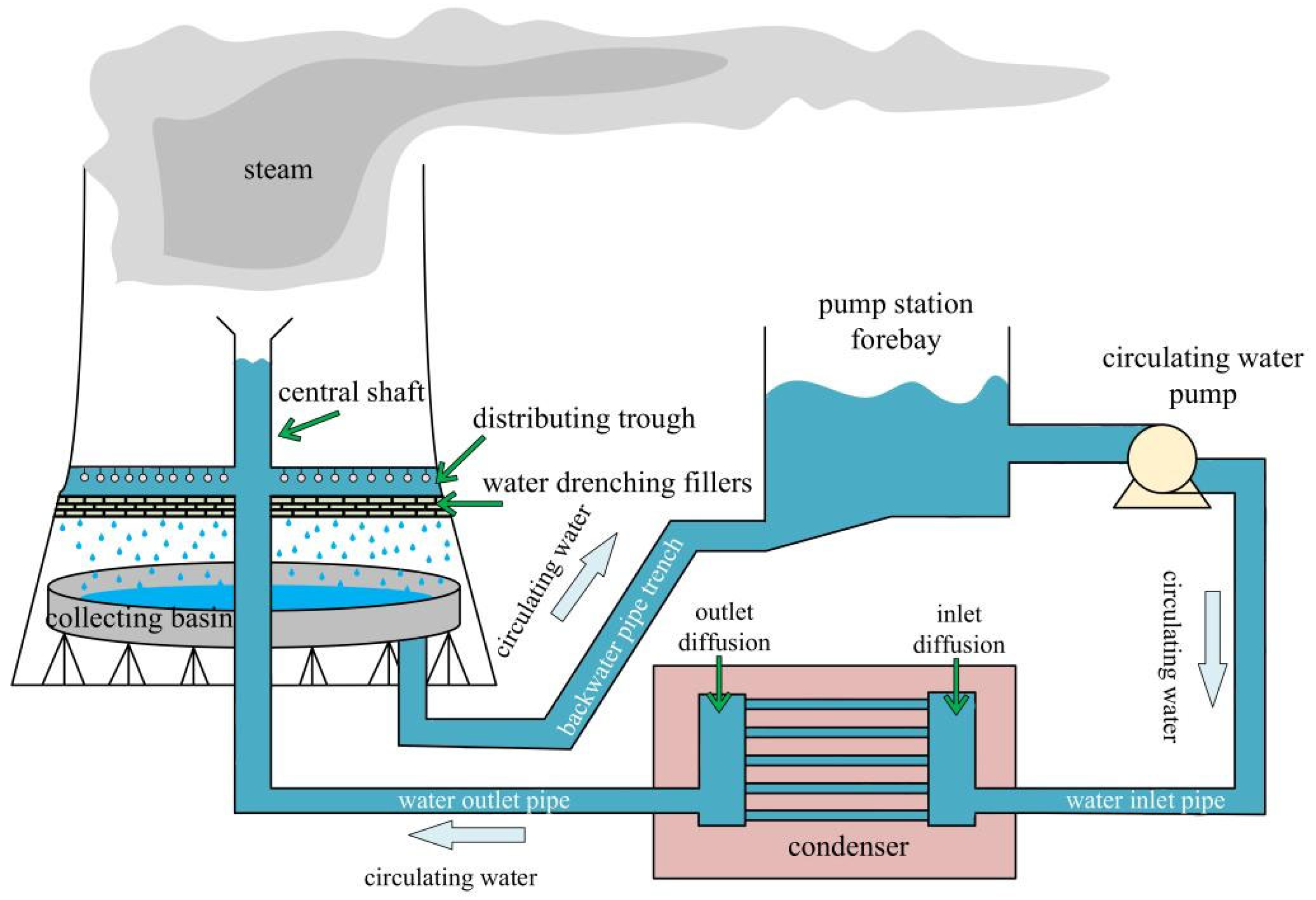
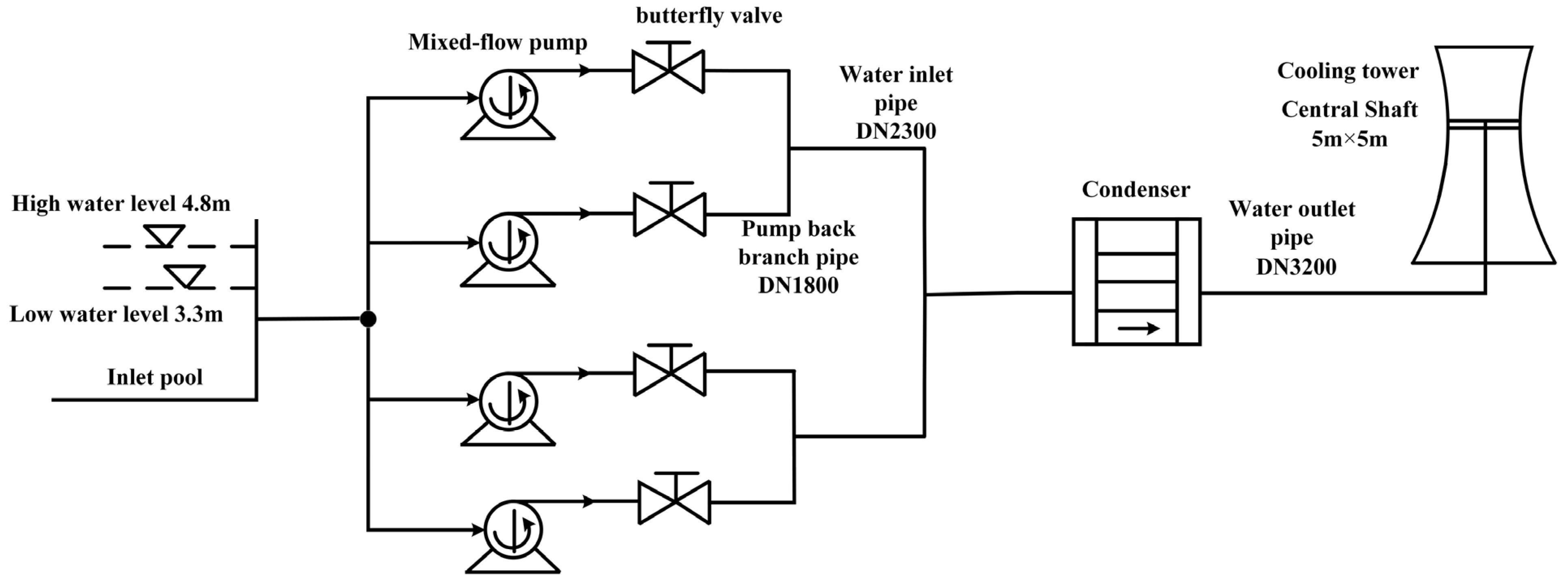
Industrial power plant circulating cooling water systems typically employ a closed-loop design to conserve water resources and reduce the environmental impact of heat emissions. The process flow is as follows: Cooling water drawn from the cooling tower’s sump is pressurized by a circulating water pump and then transported to the condenser through the inlet pipe. Inside the condenser, the cooling water absorbs the latent heat of condensation from the turbine exhaust steam, causing its temperature to rise. The heated cooling water then flows through the outlet pipe into the cooling tower shaft and rises to the tower’s water distribution system, where it is evenly sprayed onto the packing layer via nozzles. Within the packing, the water flows into full contact with forced or natural convection air, releasing heat to the atmosphere through evaporation and contact cooling, thus lowering the water temperature. The cooled water collects in the sump at the bottom of the tower and ultimately returns to the circulating water pump house inlet through the return water trench, completing a full cycle. a schematic diagram of which is shown in Figure 1.

The entire system consists of pumps, pipes, condensers, cooling towers, and various valves, filters, and other auxiliary equipment. Its reliable operation directly affects the thermal cycle efficiency and unit availability of the nuclear power plant, serving as a crucial foundation for the safe and economical operation of the nuclear power plant [26].

3. Mathematical Model

3.1. Pipeline Compatibility Equation

The dynamic characteristics of water flow in pressurized pipelines can be described by the continuity equation and motion equation of water flow, which are the basis for the calculation and analysis of water hammer in pipelines, and the forms are as follows [27]:

$${\displaystyle \frac{Q}{A}}{\displaystyle \frac{\partial H}{\partial x}}+{\displaystyle \frac{\partial H}{\partial t}}+{\displaystyle \frac{a^2}{gA}}{\displaystyle \frac{\partial Q}{\partial x}}+{\displaystyle \frac{Q}{A}}\sin \alpha =0$$

(1)

$$g{\displaystyle \frac{\partial H}{\partial x}}+{\displaystyle \frac{Q}{A^2}}{\displaystyle \frac{\partial Q}{\partial x}}+{\displaystyle \frac{1}{A}}{\displaystyle \frac{\partial Q}{\partial t}}+{\displaystyle \frac{fQ\left|Q\right|}{2D{A}^2}}=0$$

(2)

In the formula: H is the piezometric head, m; Q is the flow rate, m³/s; D is the pipe diameter, m; A is the pipe cross-sectional area, m²; t is time, s; a is the water hammer wave velocity, m/s; g is the gravitational acceleration, m/s²; x is the distance along the pipe axis, m; f is the friction coefficient; α is the angle between the pipe axis and the horizontal plane, rad.

The above two equations are a nonlinear hyperbolic partial differential equation system. Using the method of characteristics, they can be rearranged into the following finite difference equations, also known as the compatibility equations [28].

$$C^{+}:H_{pi}=C_p-B_p{Q}_{pi}$$

(3)

$$C^{-}:H_{pi}=C_m+B_m{Q}_{pi}$$

(4)

In the formula: H_pi and Q_pi are the unknown head and flow rate at section i in the pipe at time t; $C_p=H_{i-1}+B{Q}_{i-1}$; $C_m=H_{i+1}-B{Q}_{i+1}$; $B_p=B+R\left|Q_{i-1}\right|$; $B_m=B+R\left|Q_{i+1}\right|$; $B_m=B+R\left|Q_{i+1}\right|$; $B=a/gA$; $R=f\Delta x/\left(2gD{A}^2\right)$; $\Delta x=a\Delta t$; H_i−1 and Q_i−1 are the known head and flow rate at section i − 1 in the pipe at time t; H_i+1 and Q_i+1 are the known head and flow rate at section i + 1 in the pipe at time t; Δt represents the time step.

3.2. Condenser

The condenser is a crucial heat exchange device in industrial power plants, consisting of inlet and outlet water tanks and numerous parallel, slender condenser tubes. Cooling water flows into the condenser tube bundle from the inlet water tank, exchanges heat with the high-temperature exhaust gas from the turbine, and then flows out from the outlet water tank.

In the analysis of hydraulic transient processes, the condenser’s inlet and outlet water tanks can be considered equivalent to concentrated flow capacity elements, while the tens of thousands of parallel condenser tubes can be equivalent to a single elastic pipe. The equivalence principles are: ① the cross-sectional area of the equivalent tube is equal to the sum of the cross-sectional areas of all condenser tubes; ② the head loss of the equivalent tube is the same as that of a single condenser tube; ③ the length of the equivalent tube is the same as that of a single condenser tube [29].

3.3. Cooling Tower

The cooling tower serves as the downstream boundary condition in the circulating cooling water system of an industrial power plant, and the rationality of its modeling directly affects the reliability of the simulation results for hydraulic transient processes. Water flows from the inlet pipe at the bottom of the cooling tower into the central shaft, then from the distribution trough (pipe) at a higher point inside the tower to the nozzles, and finally sprays onto the packing material inside the tower. Based on the water flow characteristics in the aforementioned cooling tower, this paper studies the following four equivalent models. Model A (constant water level model) can be considered as the limiting case when the cross-sectional area of the surge tank approaches infinity, transforming it into a constant water level boundary; Model B (bidirectional surge tank model) corresponds to the classic impedance-type surge tank, preserving the dynamic changes in water level and impedance loss; Model C (branch water tower model) achieves a detailed characterization of the physical processes of high-level outflow and free overflow by introducing the weir flow formula and piecewise parameterization; Model D (composite structure model) can be understood as coupling Model B with an equivalent pipe section.

From the perspective of mechanical coupling, the interaction between cooling tower water level fluctuations and pipeline water hammer waves determines the damping characteristics and pressure extremes of the system fluctuations. Without coupling, it is impossible to accurately capture the dynamic response caused by wave reflection. Among them, the mass and momentum conservation framework based on the method of characteristics (MOC) is a general element, while the cross-sectional area of the shaft, the geometric parameters of the weir flow, and the equivalent properties of the water distribution pipe are specific items that need to be reparameterized according to the specific engineering structure.

(1)

Equivalent Model A

Reference [30] points out that the circulating cooling water system has a short pipeline and fast water hammer fluctuation. The extreme value of water hammer pressure usually occurs within the first cycle of the water hammer wave. To simplify the calculation, the cooling tower can be regarded as a reservoir with a constant water level, that is, the water level of the central shaft is assumed to be equal to the full water level of the entire tower.

$$H_p=H_s=Const$$

(5)

In the formula: H_p is the water head of the outlet pressure test pipe at the end of the inlet pipe, m; H_s is the operating water level under 100% full-tower water distribution conditions in the vertical shaft, m.

Substituting Equation (5) into Equation (3) C⁺ compatibility equation, we can obtain the flow rate Q_p at the end of the pipeline leading into the tower.

In the hydraulic transition process of a circulating cooling water system, Model A is applicable without considering the fluctuation of the cooling tower shaft water level, or under specific conditions (such as a large shaft volume), it can also be regarded as a physically reasonable boundary condition. However, since it does not consider the fluctuation of the shaft water level and treats it as a constant high water level, its water hammer calculation results are conservative, but attention should be paid to whether the reverse rotation speed of the water pump meets the safety requirements.

(2)

Equivalent Model B

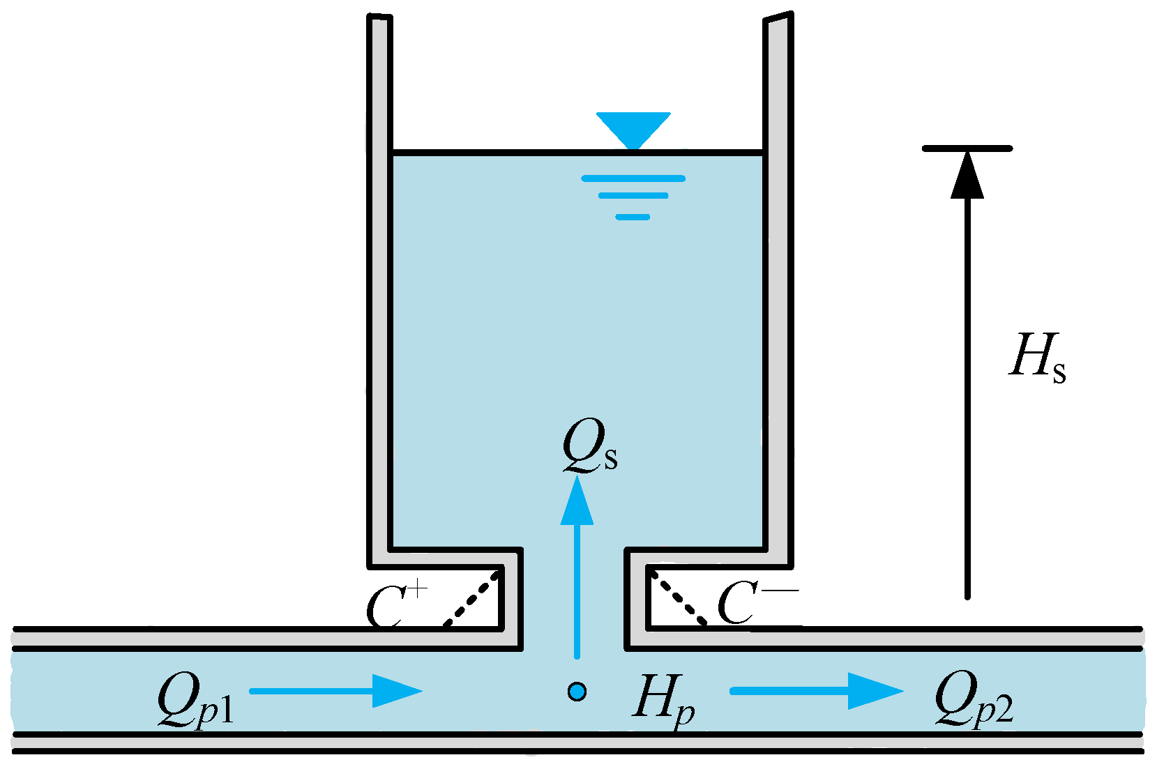
Reference [31] equates the boundary conditions of a cooling tower to those of a voltage regulating tower. As shown in Figure 2, the following equation can be obtained:

$$d{H}_s/dt=Q_s/A_s$$

(6)

$$H_p=H_s+R_k{Q}_s\left|Q_s\right|$$

(7)

$$Q_{p1}=Q_s+Q_{p2}$$

(8)

$$H_p=C_{p1}-B_{p1}{Q}_{p1}$$

(9)

$$H_p=C_{M1}+B_{M2}{Q}_{p2}$$

(10)

In the formula: A_s is the cross-sectional area of the vertical shaft, m²; Q_s is the flow rate at the inlet and outlet of the cooling tower, m³/s; R_k is the impedance head loss coefficient, $R_k=\mathsf{\Delta }{h}_s/Q_s^2$, the value of R_k is different when the water flows into and out of the impedance hole; H_p is the transient head at the pipe boundary, m; Q_p1 and Q_p2 are the transient flow rates at the pipe boundary, m³/s.

In water hammer calculations, the value of Δt is very small and can be ignored. Substituting Equations (6)–(10) into the pipeline compatibility equation, H_p can be solved, and then each transient characteristic value can be solved.

(3)

Equivalent Model C

The cooling tower is considered as a water tower with two branches. Based on the relative relationship between the water level H_s in the cooling tower shaft and the top and bottom elevations of the distribution trough, the transition process is calculated in three cases.

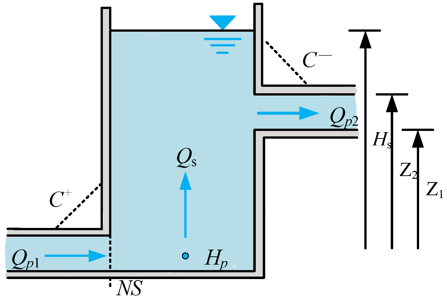
As shown in Figure 3, the two-branch water tower has two branches: Branch 1 is the bottom inlet pipe, through which water flows into the water tank; Branch 2 is the outlet of the distribution trough, through which water flows out. Z₁ is the bottom elevation of the distribution trough, and Z₂ is the top elevation of the distribution trough.

The relationship between water level changes and internal flow rate in a vertical shaft is as follows:

$$A_s{\displaystyle \frac{d{H}_s}{dt}}=Q_s$$

(11)

Integrating both sides of the above equation with respect to time t, can get:

$$H_s=H_s^0+{\displaystyle \frac{(Q_s+Q_s^0)}{2A_s}}\Delta t$$

(12)

In the formula: Q_p1 is the flow rate flowing into the vertical shaft of branch 1, m³/s; Q_p2 is the flow rate flowing out of the distribution tank, m³/s; Δt is the time step used in the calculation, s; parameters with a superscript of 0 represent known quantities at time t − Δt.

Scenario 1: When the water level in the cooling tower is higher than the top of the water distribution tank, i.e., $H_{\mathrm{s}}\ge Z_2$, branch 2 is in a pressurized full-pipe outflow state. Since the inertia and hydraulic losses of the water flow in the cooling tower shaft are negligible compared with those in the circulating water system pipes, it can be approximately assumed that the water head in the pressure measuring pipe at the bottom of the shaft is equal to the water level in the shaft.

$$H_p=H_{p1,NS}=H_s$$

(13)

In the formula: H_p is the water head of the pressure measuring pipe at the bottom of the cooling tower shaft, m; H_p1,NS is determined by the compatibility equation C⁺.

The mathematical model for Case 1 differs from that of Equivalent Model B only in the following aspect: Equivalent Model B needs to consider the head loss caused by the impedance orifice, while the two branch water towers in Case 1 do not have head loss due to the identical upper and lower cross sections. Apart from this, the two models are identical.

Scenario 2: When the water level in the water tower is between the top and bottom of branch 2, i.e., $Z_1<H_s\le Z_2$, branch 2 is in a partially submerged state. In this case, the weir flow formula can be used to calculate the flow rate of branch 2:

$$Q_{p2}=C_d{A}_e\sqrt{2g}{h}^{1/2}$$

(14)

$$C_d=0.32+0.01\left[{\displaystyle \frac{3-Z_1/(Z_2-Z_1)}{0.46+0.75Z_1/(Z_2-Z_1)}}\right]$$

(15)

In the formula: C_d is the weir flow coefficient, considering this as a right-angle flow through a broad-crested weir, the above calculation formula applies to $0\le Z_1/(Z_2-Z_1)\le 3$. For $Z_1/(Z_2-Z_1)>3$, the constant 0.32 is used [32]; A_e is the water flow area, m²; g is the gravitational acceleration, m/s²; h is the effective water depth, $h=H_s-Z_1$, m.

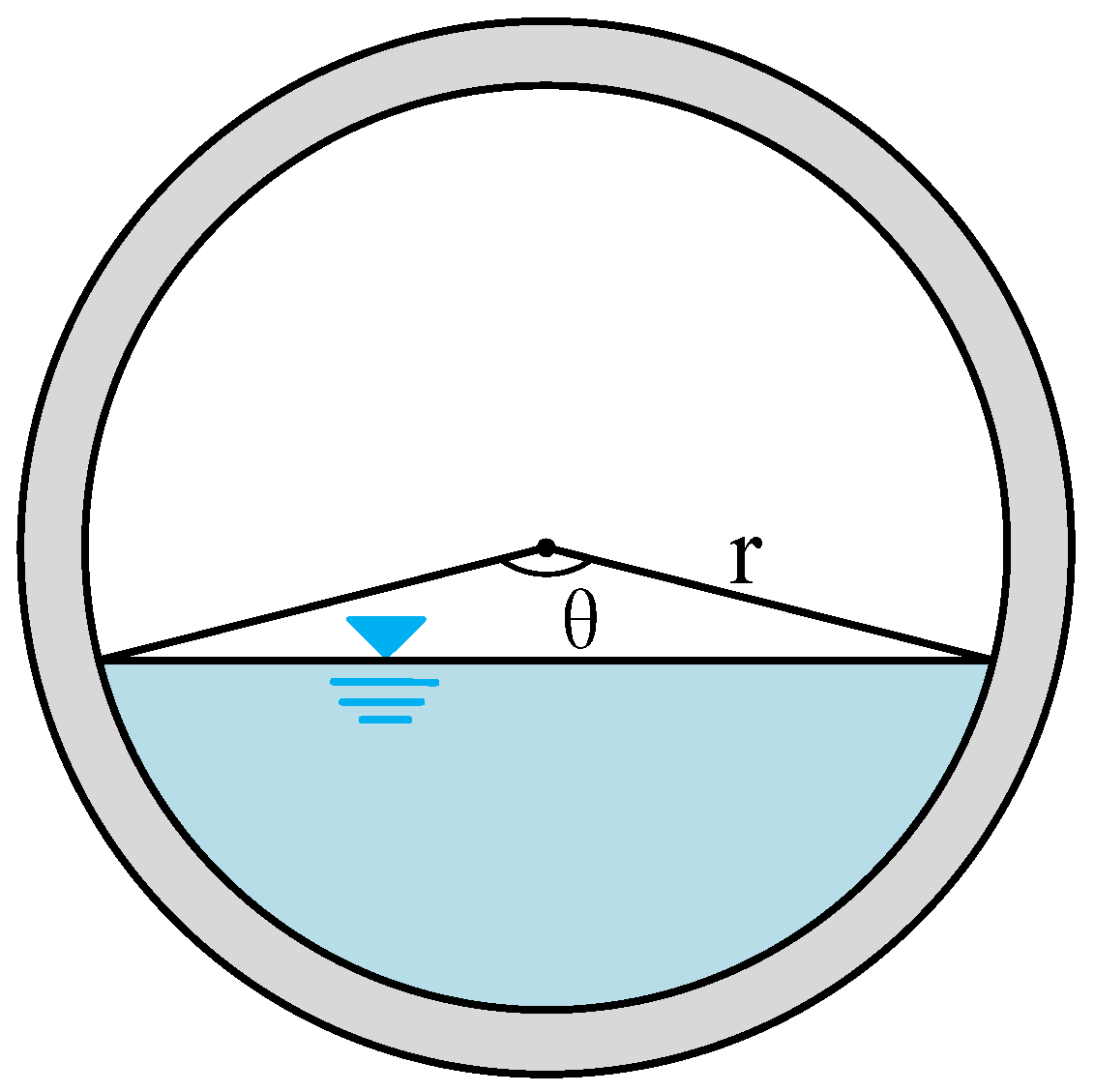
As shown in Figure 4, when the flow cross-section is a partially submerged circular pipe, its effective flow area is:

$$A_e={\displaystyle \frac{\pi D_1^2}{4}}{\displaystyle \frac{(\theta -\sin \theta )}{2\pi }}$$

(16)

$$\theta =2\arccos \left({\displaystyle \frac{r-(H_s-Z_1)}{r}}\right),r={\displaystyle \frac{D_1}{2}}$$

(17)

In the formula: D₁ is the diameter of the water distribution trough pipe, m; r is the radius of the water distribution trough pipe, m; θ is the arc corresponding to the water surface, rad.

If the cross-section is rectangular, then:

$$A_e=b(H_s-Z_1)$$

(18)

In the formula: b is the equivalent weir width of branch 2, m.

For cooling tower water distribution channels, which are generally rectangular in cross-section, the combined Equations (14) and (18) are:

$$Q_{p2}=C_d{A}_e\sqrt{2g}{h}^{1/2}=C_{d}b\sqrt{2g}{(H_s-Z_1)}^{3/2}$$

(19)

Based on the continuity of water flow at the bottom of the shaft, we can obtain:

$$Q_s=Q_{p1}-Q_{p2}$$

(20)

Substituting Equations (3) and (19) into Equation (20), can get:

$$Q_s={\displaystyle \frac{\left(H_s-C_p\right)}{B_p}}-C_{d}b\sqrt{2g}{(H_s-Z_1)}^{3/2}$$

(21)

Substituting Equation (12) into Equation (20) above for time discretization, we can rearrange it into a nonlinear equation and then solve it through Newton-Raphson iteration to obtain the transient eigenvalues.

Scenario 3: When the water level in the vertical shaft drops below the distribution tank, Q₂ equals zero and is never allowed to be less than zero, meaning there is no backflow in the distribution tank, equivalent to having a check valve installed at the distribution tank. That is, when $H_s<Z_2$, the water flow continuity condition is:

$$Q_s=Q_{p1}$$

(22)

Substituting it into Equation (11) and integrating over time t, can get:

$$H_s=H_s^0+{\displaystyle \frac{(Q_{P1}+Q_{P1}^0)}{2A_s}}\Delta t$$

(23)

By combining Equations (22) and (23) into a system of pipeline compatibility equations, the transient characteristic values can be obtained.

(4)

Equivalent Model D

Model D assumes that the water level drop in the vertical shaft during hydraulic transients is limited and will not fall below the bottom elevation of the distribution trough. Therefore, the central vertical shaft of the cooling tower can be divided into two sections: the part below the bottom elevation of the distribution trough is equivalent to an equivalent pipe, and the part above the bottom elevation of the distribution trough is equivalent to a bidirectional pressure regulating tower.

The boundary between the equivalent pipeline and the regulating chamber is set at the elevation of the bottom surface of the water distribution tank. The physical basis for this is as follows: the section below the bottom surface of the water distribution tank is always in a full-flow state during normal operation and transient processes, exhibiting obvious characteristics of a pressurized pipeline. After a pump shutdown due to an accident, the pressure wave propagates along this section at the speed of sound, with a rapid pressure response and significant amplitude. The section above the bottom surface of the water distribution tank, during normal operation, is an open channel or not a full-flow zone, with a free liquid surface; after a power outage, the liquid surface can fluctuate up and down, playing a role in storage and regulation, effectively reflecting the physical behavior of the cooling tower after a pump shutdown due to an accident.

4. Hydraulic Transient Process Calculation

4.1. Engineering Case

The circulating cooling water system of a certain power plant adopts a secondary circulation cooling method with seawater cooling towers, configured with a hyperbolic natural ventilation cooling tower, with a wetting area of 8000 m². The system is equipped with four circulating water pumps, centrally arranged in the same pump room; the pump room has a total of eight intake channels, with every two channels corresponding to one circulating water pump. The circulating water pumps selected are metal axial flow pumps, with a single pump rated flow of 5.38 m³/s and a rated head of 33 m. The normal operating water level in the pump room is 4.8 m, while the minimum operating water level is 3.3 m.

The condenser has a heat exchange area of 42,000 m², with a top elevation of 12.6 m. The circulating water is gathered from two DN1800 inlet main pipes into one DN3200 outlet main pipe, with a total pipeline length of 426 m, using round concrete pipes lined with fiberglass. The outlet pipe is connected to a vertical shaft with a cross-section size of 5.0 m × 5.0 m, and the top elevation of the shaft is 16.00 m. Above the shaft is a double-layer distribution trough, measuring 1.5 m × 3.0 m, responsible for supplying water to the cooling tower. The operating water level of the cooling tower under 100% full tower water supply conditions is 18.50 m, while the operating water level under 60% peripheral water supply conditions is 18.46 m. Figure 5 shows its simplified diagram.

4.2. Operating Condition Selection

During the operation of a circulating water system, power outages or pump startups can easily trigger rapid pressure changes within the pipelines, potentially inducing water hammer under certain conditions. To ensure system safety, it is necessary to analyze and calculate the hydraulic transient process under different water levels and flow rates, based on design requirements.

In water hammer studies of nuclear power plant circulating water systems, the scenario of a complete pump shutdown is typically the focus of analysis. This scenario is most prone to causing severe hydraulic shocks and complex pressure fluctuations, potentially leading to the most serious water hammer effect. It represents the worst design baseline scenario threatening system integrity and nuclear safety, posing the greatest risk to system safety. Although its probability of occurrence is low, its consequences are severe once it occurs; therefore, in-depth research on this scenario is crucial for ensuring the safe and stable operation of nuclear power plants.

To suppress the water hammer effect in the circulating water system under the scenario of a complete pump shutdown and to ensure the structural safety of pipelines and equipment, the circulating water pump outlet butterfly valve adopts an optimized two-stage slow-closing control mechanism. The first stage involves a rapid initial closure, adjusting the valve from 100% open to 20° within 30 s to quickly suppress the development of reverse flow in the pipeline. The second stage switches to a gradual closure mode, gradually closing the valve from 20° to full closure within 60 s to avoid secondary positive pressure water hammer caused by a sudden drop in flow velocity. This control strategy suppresses pump reversal and reverse flow impact through rapid initial valve closure, and weakens the superposition effect of pressure waves through gradual closure, thereby effectively controlling the risk of water hammer.

4.3. Transient Process Analysis Under Different Equivalent Models

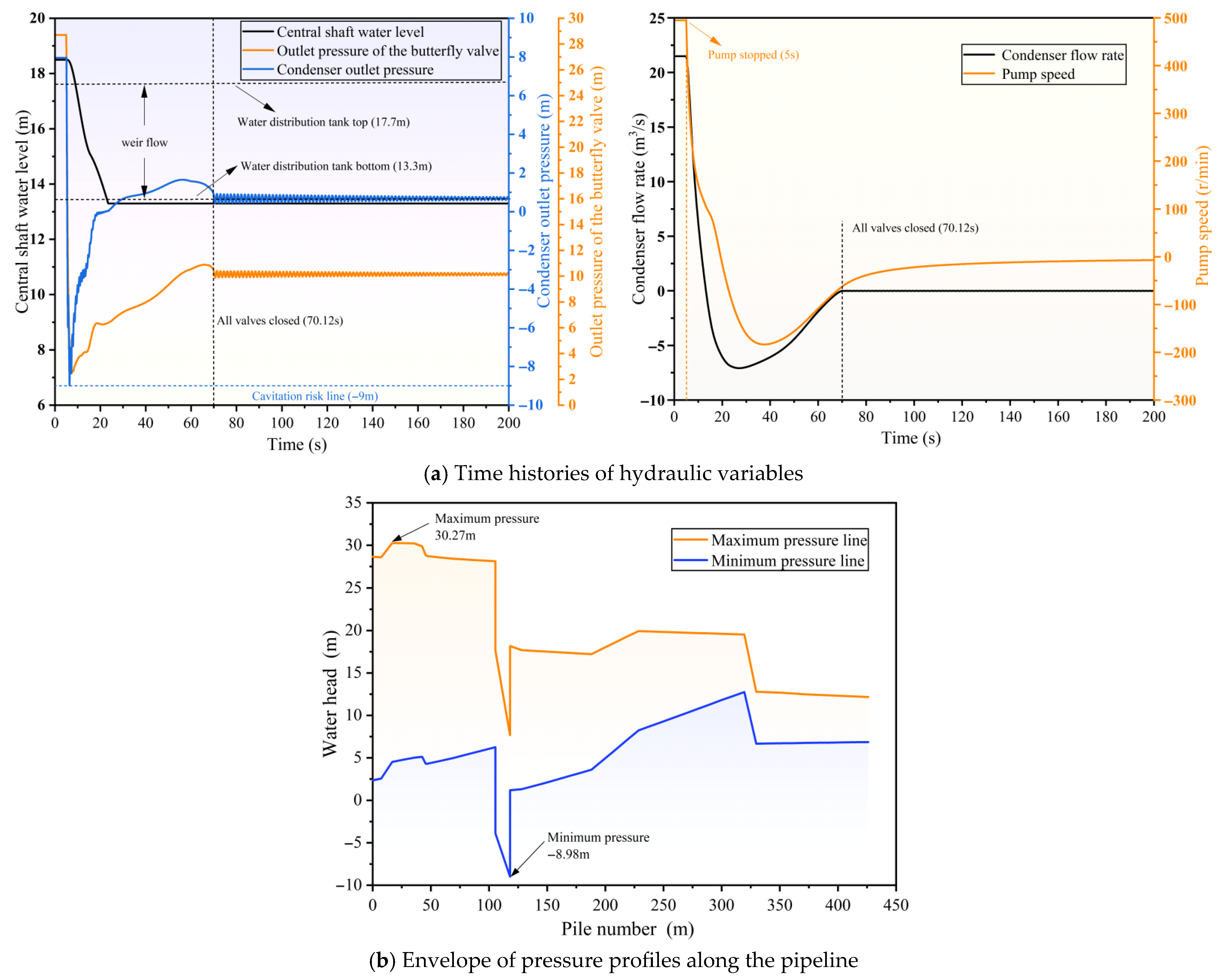
To address the adverse condition of simultaneous power failure of four circulating water pumps, numerical simulations were conducted using four different equivalent cooling tower models to obtain the time-domain variations of parameters such as circulating water pump speed and flow rate, valve outlet pressure head, condenser outlet pressure head, and cooling tower shaft water level under the accidental pump stop condition.

4.3.1. Analysis of Results from Equivalent Model A

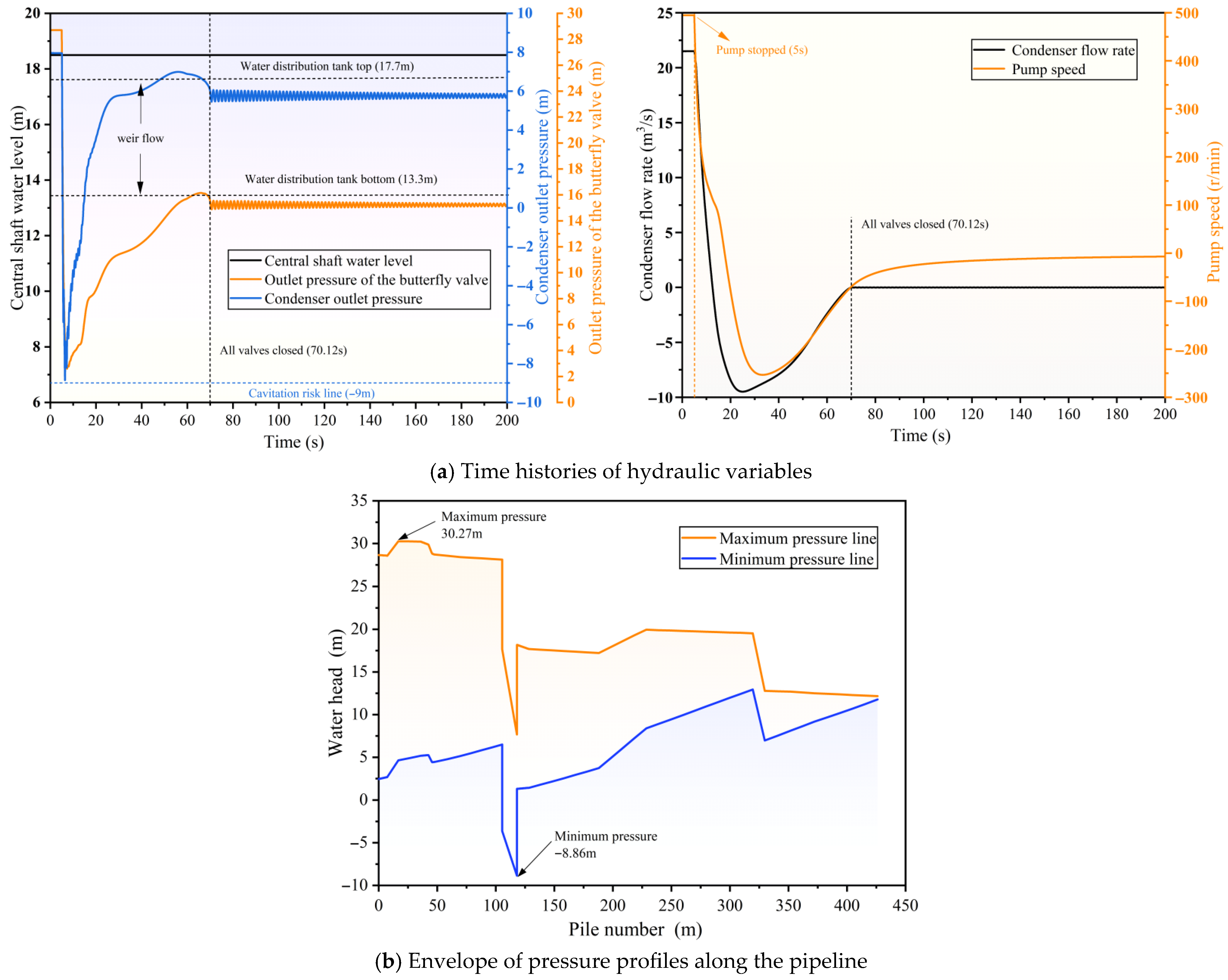
Model A employs maximum simplification, treating the central shaft of the cooling tower as a constant water level in transient calculations. It is assumed that the shaft water level remains constant at the full-capacity operating level (18.50 m). At the moment of power failure, the pump loses its driving torque. Due to inertia, the water flow in the pipes causes the pump to continue rotating forward while gradually decelerating. Pressure fluctuations occur upstream (butterfly valve outlet) due to water flow inertia, while negative pressure appears downstream (condenser outlet) due to a sudden drop in flow. Since the shaft water level is assumed to be constant, the system consistently receives a stable high-level water supply. This causes the pump to reverse direction after its speed returns to zero, driven by the pressure difference, resulting in a large reverse flow and reverse speed. As shown in

Table 1. Computed characteristic values of Model A under accidental pump trip.

Eigenvalues	Maximum Value	Minimum Value
butterfly valve outlet pressure (m)	28.71	2.61
condenser outlet pressure (m)	7.96	−8.86
condenser flow rate (m3/s)	21.50	−9.49
water pump speed (r/min)	495	−253.24
central shaft water level (m)	18.50	18.50
along the way (m)	30.27	−8.86

, the maximum outlet pressure of the butterfly valve is 28.71 m, and the minimum outlet pressure of the condenser reaches −8.86 m, indicating a significant negative pressure. The pump speed drops to a minimum of −253.24 r/min, with the most severe reversal among the four models. The minimum condenser flow rate also reaches −9.49 m³/s, with the largest reverse flow. Figure 6 shows the calculation results.

In summary, Model A, by assuming a constant water level in the shaft, effectively provides the pipeline with unlimited water replenishment capacity. This leads to a continuous pressure differential driving the pump to reverse, resulting in both the reverse rotation speed and the reverse flow rate being excessively high. This model is overly conservative and fails to accurately reflect the buffering effect of a dynamic drop in the shaft water level on the system. It is suitable as a conservative reference for engineering safety verification.

4.3.2. Analysis of Results from Equivalent Model B

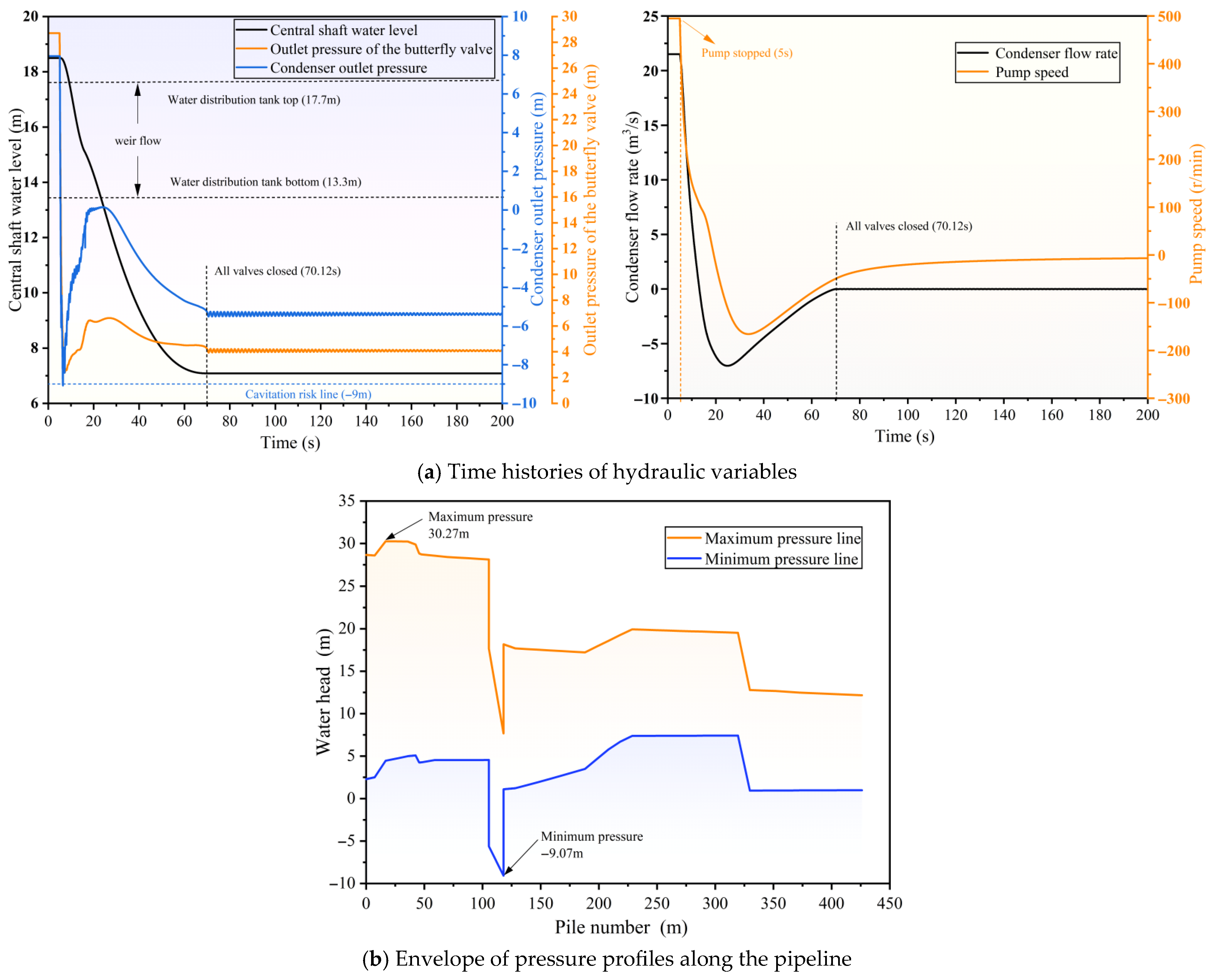
Model B simplifies the central shaft of the cooling tower as a bidirectional pressure regulating tower. After a power outage, the pump speed drops rapidly, and the pipeline flow decreases. When the pipeline pressure drops, the pressure regulating tower replenishes water to suppress the increase of negative pressure. Conversely, when the pipeline pressure rises, water can flow back into the pressure regulating tower, reducing positive pressure. The water level in the shaft rises and falls dynamically with the inflow and outflow of water. However, this model only considers the inflow and outflow characteristics of the low-level circulating water and fails to simulate the process of water flowing out of the shaft through the distribution channel at the corresponding height. This results in an underestimated outflow height and neglects the pressure differential driven by the replenishment water. As shown in

Table 2. Computed characteristic values of Model B under accidental pump trip.

Eigenvalues	Maximum Value	Minimum Value
butterfly valve outlet pressure (m)	28.72	2.43
condenser outlet pressure (m)	7.96	−9.07
condenser flow rate (m3/s)	21.50	−7.02
water pump speed (r/min)	495	−165.64
central shaft water level (m)	18.50	7.09
along the way (m)	30.27	−9.07

, the lowest water level in the vertical shaft dropped to 7.09 m, which is significantly lower than that in Model A, indicating that the dynamic water replenishment of the surge tank consumed the effective water storage in the vertical shaft; the minimum condenser outlet pressure was −9.07 m, slightly lower than that in Model A, indicating that the negative pressure was somewhat aggravated; the pump reverse rotation speed was −165.64 r/min, which is significantly lower than that in Model A, and the minimum reverse flow rate was −7.02 m³/s, indicating that the dynamic water level drop weakened the reverse driving force. Figure 7 shows the calculation results.

In summary, Model B, compared to Model A, introduces the concept of dynamic water level changes, making it closer to reality to some extent. However, because it ignores the influence of high-level outflow from the distribution channel, its simulation of the outflow characteristics of the vertical shaft has some deviations, resulting in an excessively large drop in the water level of the vertical shaft. The reliability of the calculation results still needs further improvement.

4.3.3. Analysis of Results from Equivalent Model C

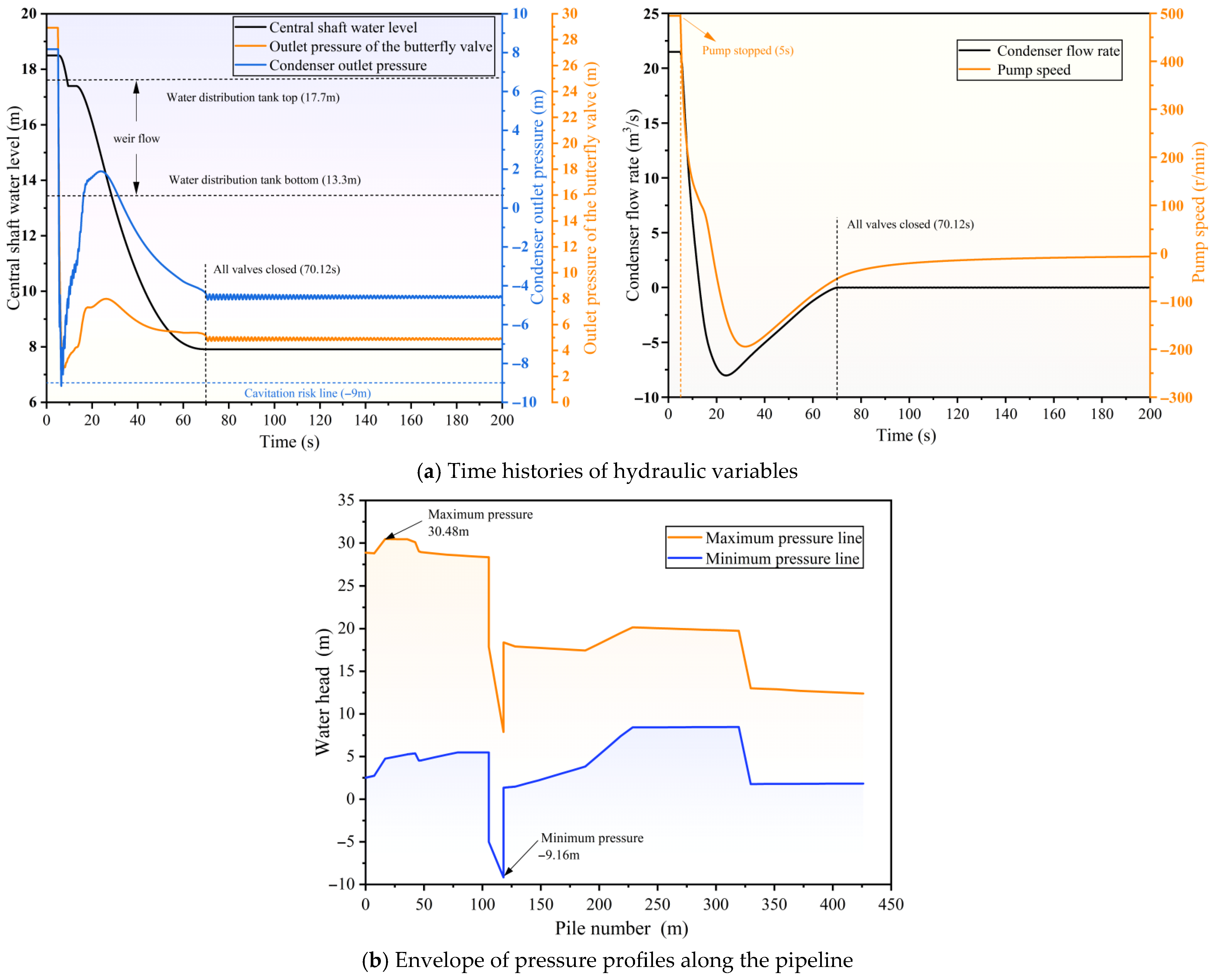
In the equivalent modeling of the central shaft of the cooling tower, Model C considers the shaft and the water distribution channel (pipe) as a whole. Water flows in from the bottom of the shaft and out through the distribution channel at the corresponding height. Based on the continuity equation of the water body in the shaft, a dynamic relationship between its water level and inflow/outflow can be established. After a pump stoppage due to an accident, the pump speed decreases, the pipeline flow decreases, and the water level in the shaft gradually drops because the outflow is greater than the inflow. This model simultaneously considers the complete path of water flowing in from the bottom of the shaft and out through the distribution channel at the corresponding height. The effective water storage capacity and outflow height of the shaft are reasonably represented, and its dynamic regulation effect on the pipeline system is more realistic. As shown in

Table 3. Computed characteristic values of Model C under accidental pump trip.

Eigenvalues	Maximum Value	Minimum Value
butterfly valve outlet pressure (m)	28.93	2.58
condenser outlet pressure (m)	8.18	−9.16
condenser flow rate (m3/s)	21.50	−8.02
water pump speed (r/min)	495	−194.47
central shaft water level (m)	18.50	7.91
along the way (m)	30.48	−9.16

, the lowest water level in the vertical shaft drops to 7.91 m, which is between the corresponding water levels in Model B and Model D; the maximum butterfly valve outlet pressure is 28.93 m, which is slightly higher than the other two models; the minimum condenser outlet pressure is −9.16 m, which is lower than the minimum value in Model A; the maximum reverse speed of the water pump is −194.47 r/min, and the degree of reverse rotation is more severe than in Model B; the minimum reverse flow rate of the condenser is −8.02 m³/s. Figure 8 shows the calculation results.

In summary, Model C achieves dynamic coupling between the inflow and outflow of the vertical shaft and the water level through the continuity equation. It can realistically reproduce the regulating characteristics of the vertical shaft during the hydraulic transition process, specifically the dynamic balance between water inflow and outflow in the “two-branch water tower” mode, and accurately reveal the negative pressure characteristics at the top of the condenser under extremely unfavorable operating conditions. Furthermore, the variation law of the vertical shaft water level is in good consistency with the actual engineering physical characteristics, indicating that the model can effectively reflect the hydraulic characteristics of the cooling tower in transient calculations, possessing high engineering applicability and simulation accuracy.

4.3.4. Analysis of Results from Equivalent Model D

Model D employs a composite structural equivalent approach, decomposing the central vertical shaft of the cooling tower into two parts: an “equivalent pipe” from the bottom of the tower to the bottom of the water distribution tank, and a “pressure regulating well” above the bottom of the water distribution tank. After a power outage, the pump speed decreases. The lower equivalent pipe section, acting as a pressurized pipeline filled with water, transmits water hammer waves, while the upper pressure regulating well buffers and regulates the pipeline pressure through the dynamic water storage and release function of the free liquid surface. The combined effect of these two parts accurately reflects the pressurized water flow characteristics at the bottom of the shaft and also demonstrates the absorption and regulation of pressure fluctuations by the upper liquid surface. As shown in

Table 4. Computed characteristic values of Model D under accidental pump trip.

Eigenvalues	Maximum Value	Minimum Value
butterfly valve outlet pressure (m)	28.71	2.49
condenser outlet pressure (m)	7.96	−8.98
condenser flow rate (m3/s)	21.50	−7.08
water pump speed (r/min)	495	−183.53
central shaft water level (m)	18.50	13.30
along the way (m)	30.27	−8.98

, the lowest water level in the shaft only drops to 13.30 m, a significant difference compared to 7.91 m in Model C, indicating that this model overestimates the shaft’s regulation capacity. In addition, the maximum outlet pressure of the butterfly valve is 28.71 m, the minimum outlet pressure of the condenser is −8.98 m, the maximum reverse speed of the water pump is −183.53 r/min, and the minimum reverse flow of the condenser is −7.08 m³/s. Figure 9 shows the calculation results.

In summary, while Model D structurally distinguishes between the pressurized lower section and the free surface upper section of the shaft, possessing some physical significance, its combination method fails to accurately reproduce the dynamic process of water flowing out of the shaft via the distribution channel. This results in a significantly optimistic simulation of the shaft’s water level variation, leading to lower calculation accuracy compared to Model C. In practical engineering applications, it is recommended to compare and verify the results of Model D with those of Model C to avoid misjudging the system’s hydraulic safety margin.

4.4. Model Comparison and Discussion

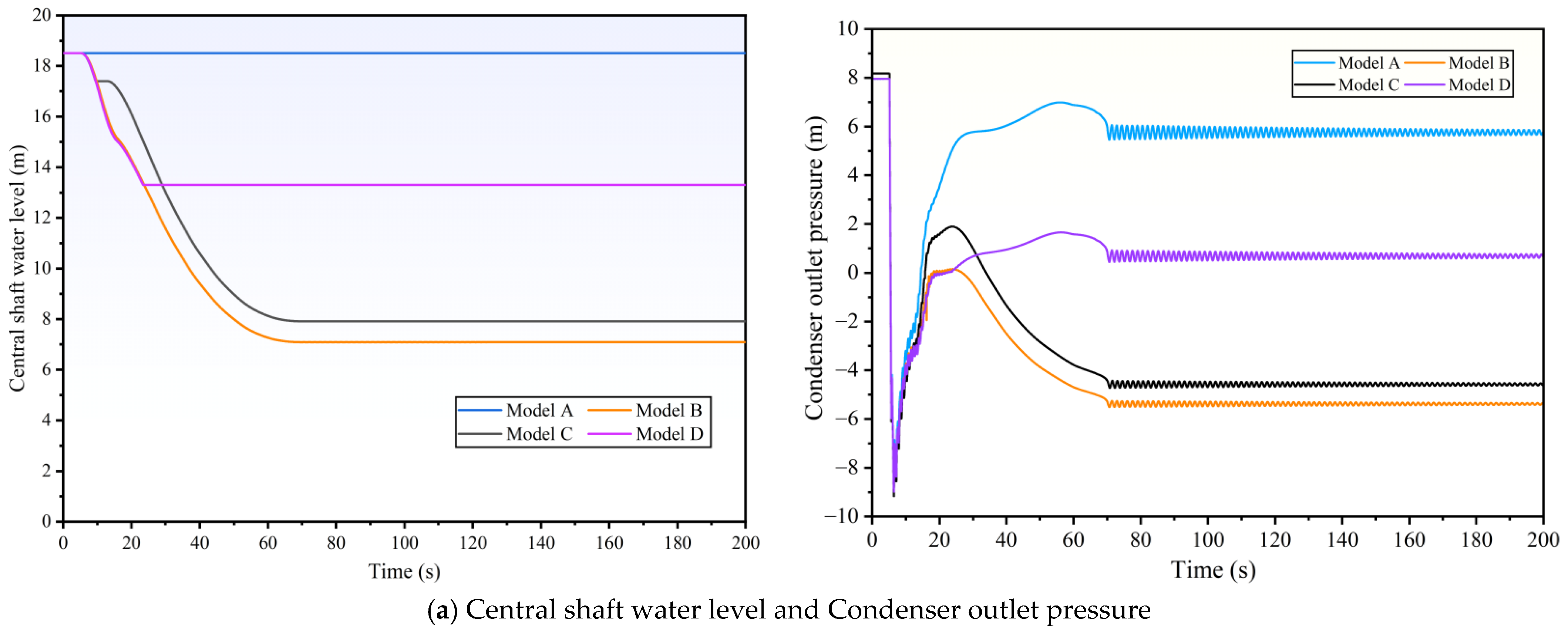
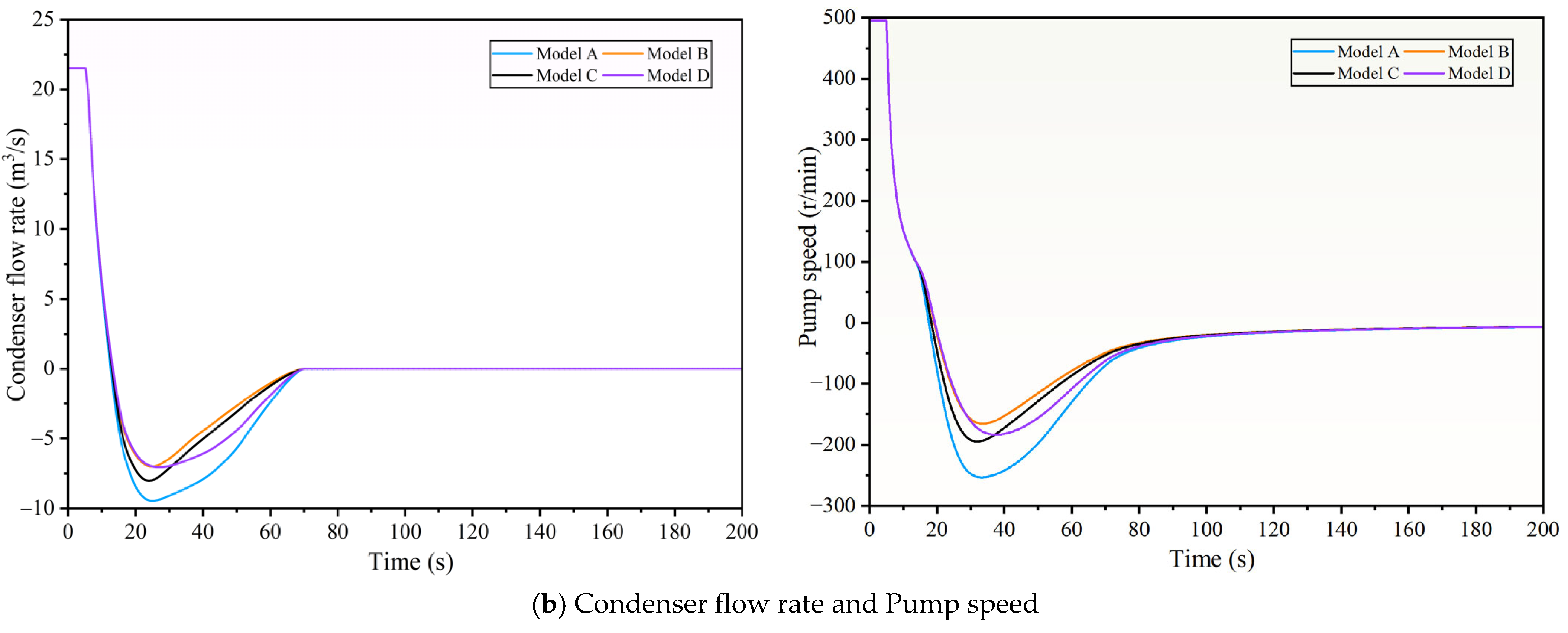
Regarding pump speed, the circulating water pumps in models A to D dropped from their rated speed to zero and began to reverse at 17.59 s, 19.2 s, 18.3 s, and 19.4 s, respectively. The speed change curves of models A to D showed a generally consistent trend. Regarding pipeline flow rate, the water flow in the circulating water pipelines began to reverse at 12.57 s, 13.2 s, 12.9 s, and 13.2 s, respectively; the maximum reverse flow rates for each model were 44.1%, 32.7%, 37.3%, and 32.9% of the rated flow rate, respectively. The flow rate change curves of models B, C, and D showed roughly the same trend.

Regarding condenser outlet pressure, all models exhibited significant pressure fluctuations within the first 10 s. Subsequently, the condenser outlet pressure of Model B and Model C showed a trend of first increasing and then decreasing after reaching the lowest point, and the minimum pressure values reached by the two were relatively close; the pressure of Model A and Model D, after increasing and then decreasing slightly, fluctuated around 5.8 m and 0.7 m respectively.

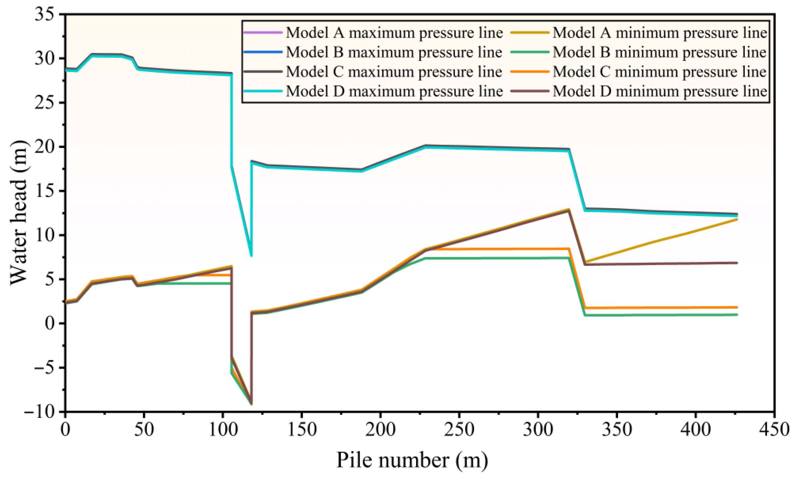
Figure 10 shows a comparison of the pressure envelopes along the flow path under different equivalent models of the cooling tower. Regarding the maximum pressure envelope, the calculation results of models A to D are basically consistent, indicating that under normal operating conditions at rated flow, the downstream boundary conditions of these four models have little impact on the transient process of the circulating cooling water system. Regarding the minimum pressure envelope, the calculation results of models B and C are almost identical. Because model D treats the portion below the distribution tank as equivalent to a pipe, due to its impedance characteristics, when the water flow stabilizes after a pump failure, the water level in the pipe is not lower than that of models B and C. Therefore, the minimum pressure envelope calculated by model D is slightly higher than that of models B and C in the latter half of the circulating water system.

From a practical engineering perspective, the central shaft of the cooling tower is located at the highest point of the circulating water system during normal operation. After a pump failure, the pump loses power instantaneously, causing backflow in the shaft and a drop in water level. After the water flow stabilizes, the water level remains between the condenser elevation (12.6 m) and the inlet pipe elevation (5.3 m).

In summary, comparative analysis of different equivalent cooling tower models shows that the calculation results of Model B and Model C generally exhibit consistent trends and are closer to actual engineering conditions. Further analysis of the vertical shaft water level fluctuation characteristics shown in Figure 11a reveals that when the vertical shaft water level drops to the elevation of the distribution channel, Model C, considering the high-level drainage characteristics, maintains the vertical shaft water level at the distribution channel elevation for a period before starting to decline, provided that the low-level inflow rate and high-level outflow rate are equal. This dynamic response process more accurately reflects the water flow characteristics of the circulating water system after a pump shutdown than Model B. Therefore, among the four compared models, Model C exhibits relatively better overall performance.

5. Sensitivity Analysis

To assess the impact of key parameters of Model C on the calculation results of the hydraulic transient process of the circulating water system and to verify the robustness of the model, this section selects four parameters—pump moment of inertia, pipe roughness, central shaft cross-sectional area, and time step—and conducts sensitivity analyses on each. The most unfavorable operating condition of simultaneous power failure of all four circulating water pumps is analyzed. By changing the target parameters one by one while keeping other conditions constant, the changes in key response indicators such as butterfly valve outlet pressure, condenser outlet pressure, condenser flow rate, pump speed, central shaft water level, and friction head are observed.

5.1. Water Pump Rotational Inertia Analysis

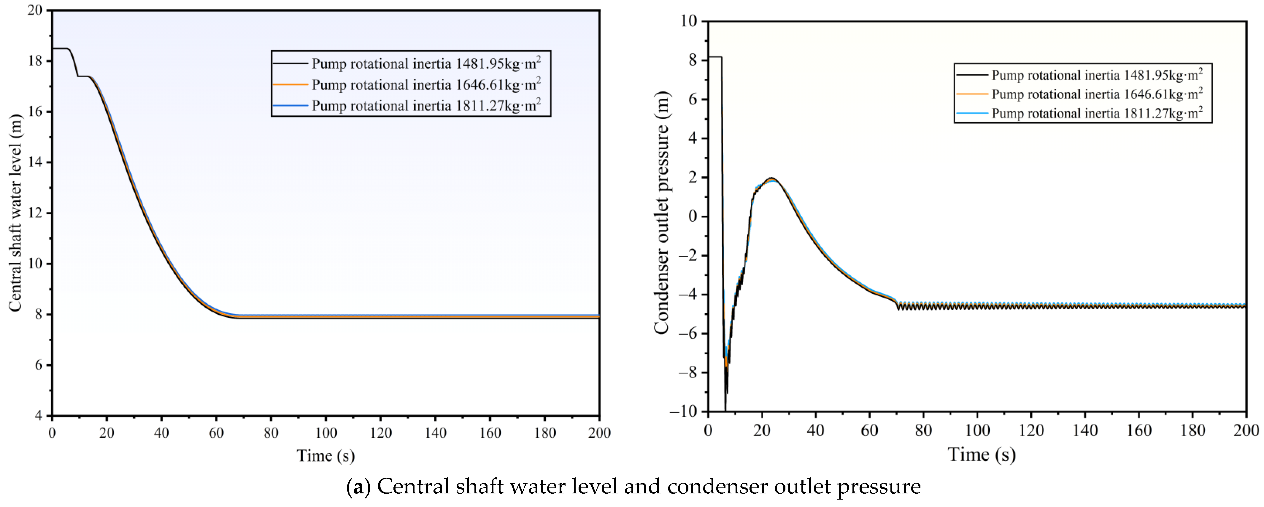
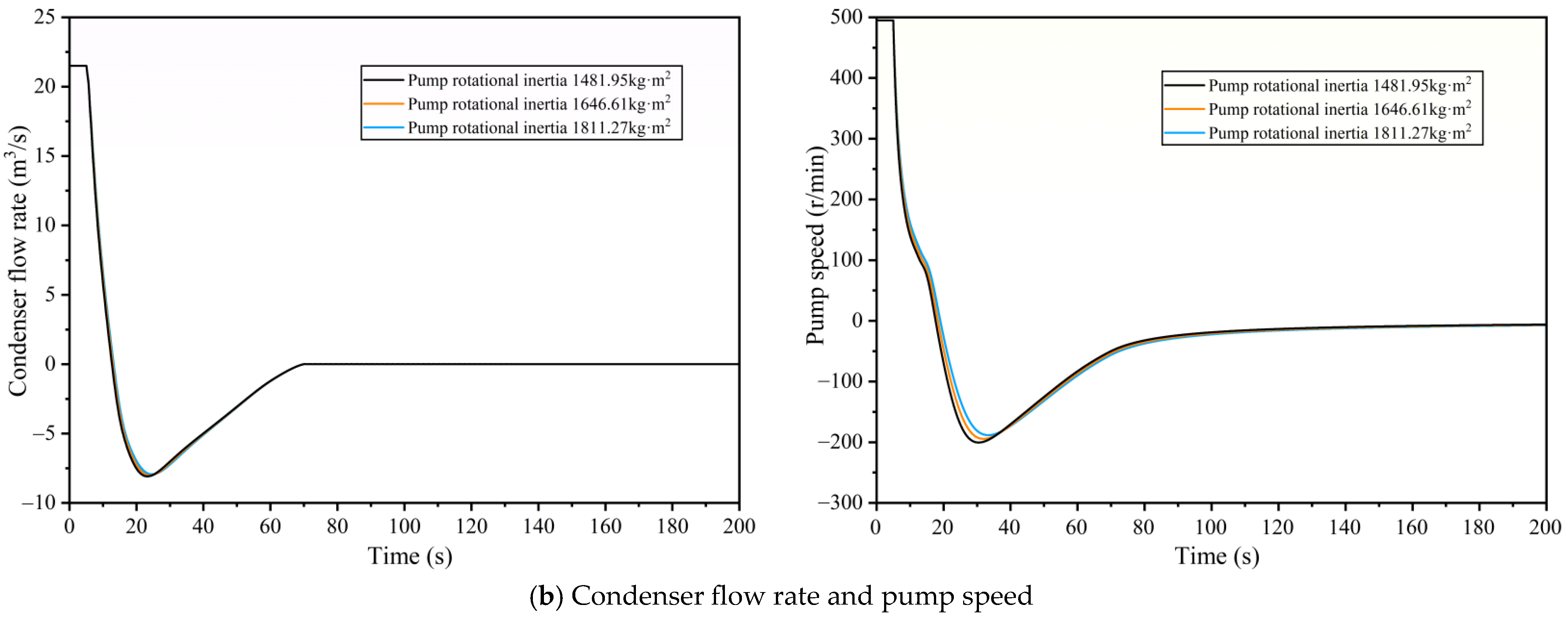
The moment of inertia of a water pump is a key mechanical parameter affecting the rate of speed decay and reverse characteristics of the pump after a pump stoppage due to an accident. This study selected two sets of moment of inertia values, 90% (1481.95 kg·m²) and 110% (1811.27 kg·m²) of the rated moment of inertia of the water pump (1646.61 kg·m²), for sensitivity analysis. The calculation results are shown in Figure 12 below.

Table 5. Sensitivity analysis of pump inertia in Model C.

Water Pump Rotational Inertia (kg·m2)	Butterfly Valve Outlet Pressure (m)		Condenser Outlet Pressure (m)		Condenser Flow Rate (m3/s)	Water Pump Speed (r/min)	Central Shaft Water Level (m)	Along the Way (m)
	Maximum Value	Minimum Value	Maximum Value	Minimum Value	Minimum Value	Minimum Value	Minimum Value	Maximum Value	Minimum Value
1481.95	28.93	1.86	8.18	−10.00	−8.09	−200.56	7.85	30.48	−10.00
1646.61	28.93	2.58	8.18	−9.16	−8.02	−194.47	7.91	30.48	−9.16
1811.27	28.93	3.20	8.18	−8.40	−7.94	−188.38	7.98	30.48	−8.40

shows that as the pump’s moment of inertia increases, the extreme conditions of the hydraulic transition process after a pump shutdown are significantly alleviated. When the moment of inertia increases from 1481.95 kg·m² to 1811.27 kg·m², the minimum butterfly valve outlet pressure increases from 1.86 m to 3.20 m, the minimum condenser outlet pressure increases from −10.00 m to −8.40 m, the extreme reverse pump speed increases from −200.56 r/min to −188.38 r/min, the minimum condenser reverse flow also increases from −8.09 m³/s to −7.94 m³/s, and the lowest water level in the central shaft slightly rises from 7.85 m to 7.98 m. This indicates that a larger moment of inertia helps to mitigate the negative pressure effect caused by a pump shutdown in the circulating water system and can appropriately reduce the rate of water level drop in the shaft. The pump’s moment of inertia has a significant impact on the minimum negative pressure along the system’s friction path but no impact on the maximum positive pressure.

The above results are due to the fact that a larger moment of inertia enhances the inertial torque of the pump rotor against changes in speed, resulting in a more gradual decrease in speed after a power outage. This slows down the reversal of water flow velocity in the pipeline, thereby reducing pressure fluctuations and extreme negative pressure caused by rapid reversal of water flow. Therefore, in practical engineering, appropriately increasing the moment of inertia of the circulating water pump can be an effective water hammer protection measure, but it is necessary to comprehensively consider equipment cost and startup characteristics.

5.2. Pipe Roughness Analysis

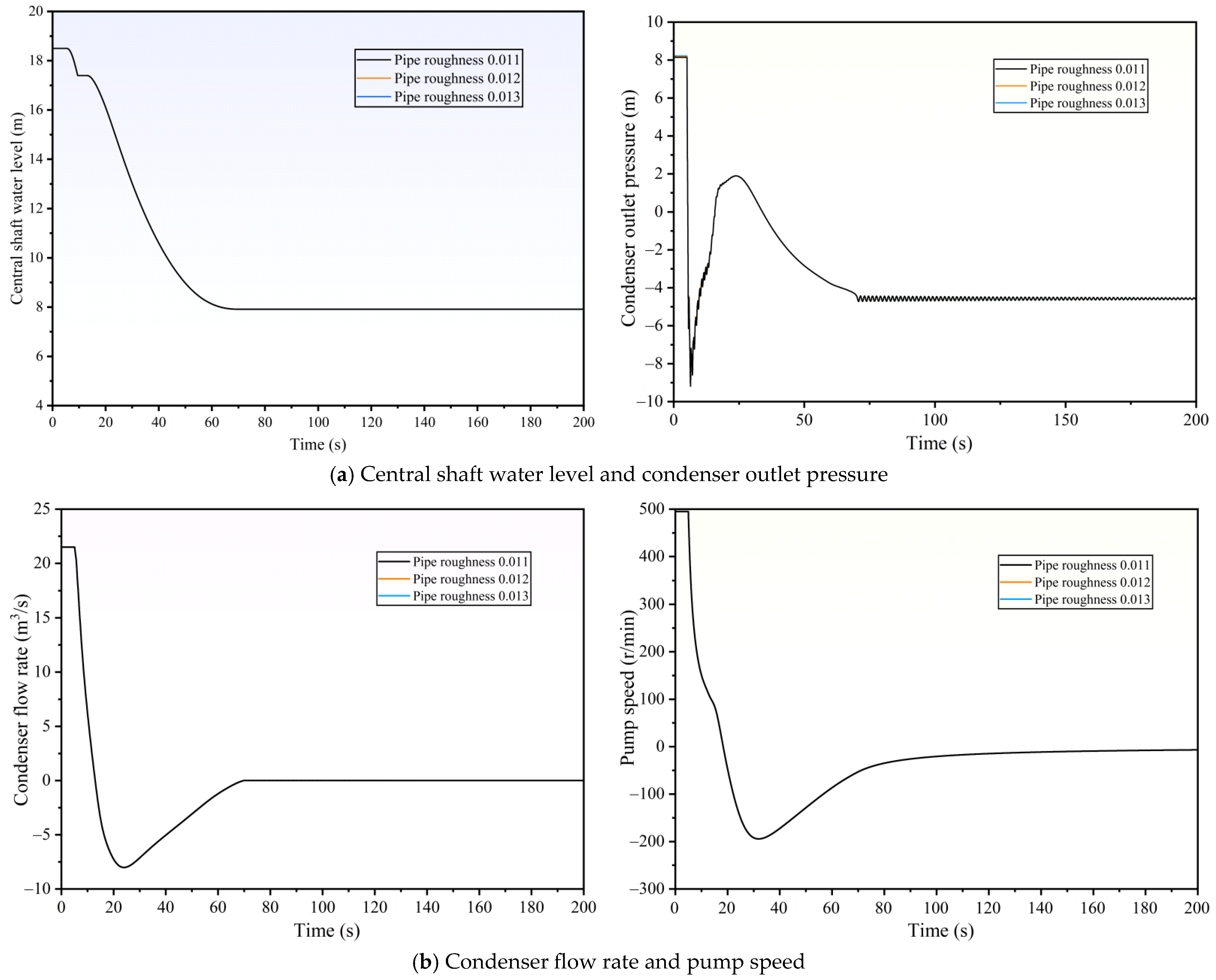
Pipe roughness directly affects the head loss along the flow path during transient flow, thereby altering the energy dissipation characteristics of the system. This study selected two sets of roughness values with rated roughness of 0.012 ± 0.001 (0.011, 0.013) for sensitivity analysis. The calculation results are shown in Figure 13 below.

Table 6. Sensitivity analysis of pipe roughness in Model C.

Pipe Roughness	Butterfly Valve Outlet Pressure (m)		Condenser Outlet Pressure (m)		Condenser Flow Rate (m3/s)	Water Pump Speed (r/min)	Central Shaft Water Level (m)	Along the Way (m)
	Maximum Value	Minimum Value	Maximum Value	Minimum Value	Minimum Value	Minimum Value	Minimum Value	Maximum Value	Minimum Value
0.011	28.89	2.56	8.14	−9.19	−8.02	−194.49	7.92	30.45	−9.19
0.012	28.93	2.58	8.18	−9.16	−8.02	−194.47	7.91	30.48	−9.16
0.013	28.97	2.61	8.22	−9.13	−8.01	−194.45	7.91	30.52	−9.13

shows that under the condition of pump shutdown due to an accident, the change in pipeline roughness has a relatively limited impact on the system hydraulic parameters. When the roughness increases from 0.011 to 0.013, the minimum butterfly valve outlet pressure slightly increases from 2.56 m to 2.61 m, the minimum condenser outlet pressure slightly improves from −9.19 m to −9.13 m, and the minimum friction head correspondingly increases from −9.19 m to −9.13 m. It is noteworthy that the minimum condenser flow rate remains stable at around −8.02 m³/s, the extreme value of the pump reverse rotation speed remains within a very small range of −194.45 r/min to −194.49 r/min, and the minimum water level in the central shaft remains basically constant at around 7.91 m.

These results indicate that during the extreme transient process of a power outage, the water hammer effect, dominated by inertial force and water level-pressure difference, has a very small impact from the change in friction resistance, and the system roughness has a very small effect on the calculation results. This is mainly because the local head loss in a short-distance circulating water system is much greater than the friction head loss. This phenomenon also indicates that the pipe resistance coefficient used in Model C has good tolerance within the range of conventional engineering values, and the calculation results are reliable.

5.3. Shaft Cross-Sectional Area Analysis

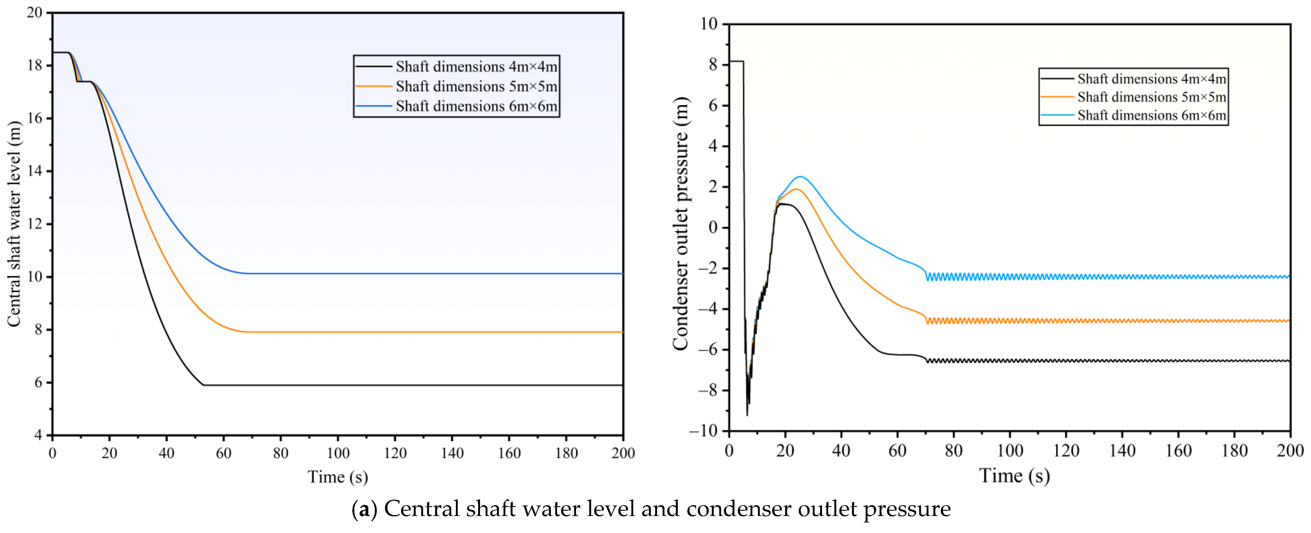
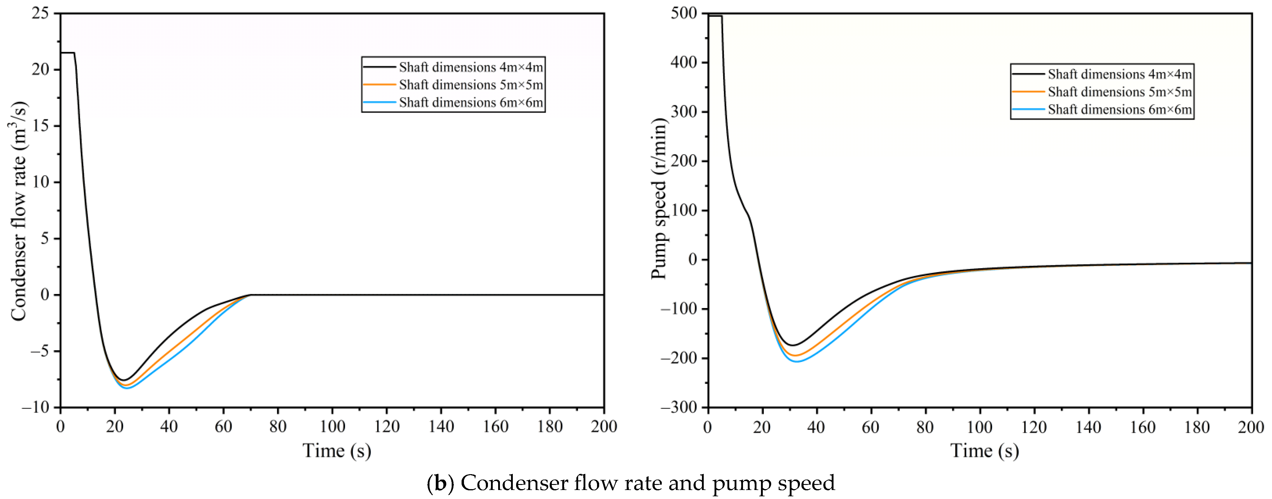
As a key regulating and storage structure in the cooling tower system, the central shaft’s cross-sectional area directly determines the water storage volume corresponding to a unit change in water level, thus affecting the system’s water replenishment and buffering capacity during pump shutdown accidents. The original shaft dimensions were 5 m × 5 m. This study selected two shaft dimensions, 4 m × 4 m and 6 m × 6 m, for sensitivity analysis, and the calculation results are shown below. The calculation results are shown In Figure 14 below.

Table 7. Sensitivity analysis of shaft cross-sectional area in Model C.

Shaft Cross-Sectional Area	Butterfly Valve Outlet Pressure (m)		Condenser Outlet Pressure (m)		Condenser Flow Rate (m3/s)	Water Pump Speed (r/min)	Central Shaft Water Level (m)	Along the Way (m)
	Maximum Value	Minimum Value	Maximum Value	Minimum Value	Minimum Value	Minimum Value	Minimum Value	Maximum Value	Minimum Value
4 m × 4 m	28.93	2.52	8.18	−9.23	−7.57	−173.85	5.9	30.48	−9.23
5 m × 5 m	28.93	2.58	8.18	−9.16	−8.02	−194.47	7.91	30.48	−9.16
6 m × 6 m	28.93	2.62	8.18	−9.12	−8.29	−206.91	10.13	30.48	−9.12

shows that as the cross-sectional area of the shaft increases, the negative pressure of the system can be appropriately alleviated, but the reverse flow phenomenon is exacerbated. Specifically, when the shaft size increases from 4 m × 4 m to 6 m × 6 m, the minimum condenser outlet pressure improves from −9.23 m to −9.12 m, and the minimum water level in the central shaft increases significantly from 5.90 m to 10.13 m, indicating that the larger shaft cross-sectional area provides more ample water storage, suppressing the excessively rapid drop in water level. However, the extreme value of the pump reverse speed increases from −173.85 r/min to −206.91 r/min, and the minimum condenser reverse flow rate increases from −7.57 m³/s to −8.29 m³/s. This exacerbation of the reverse trend can be explained by the fact that the larger shaft cross-sectional area can continuously provide a larger reverse pressure differential when the system experiences negative pressure, prompting the water flow to enter the reverse flow state more quickly.

In summary, increasing the cross-sectional area of the vertical shaft is beneficial for suppressing the negative pressure at the condenser outlet and preventing the water column from breaking, but it will exacerbate the degree of pump reversal and reverse flow. In engineering design, a balance needs to be struck between negative pressure protection and reversal suppression; this can also be combined with optimization of the pump outlet valve closing procedure. From the perspective of the simulation accuracy of Model C, this sensitivity law is consistent with physical expectations, further verifying the rationality of Model C in characterizing the dynamic regulation and storage characteristics of the vertical shaft.

5.4. Time Step Analysis

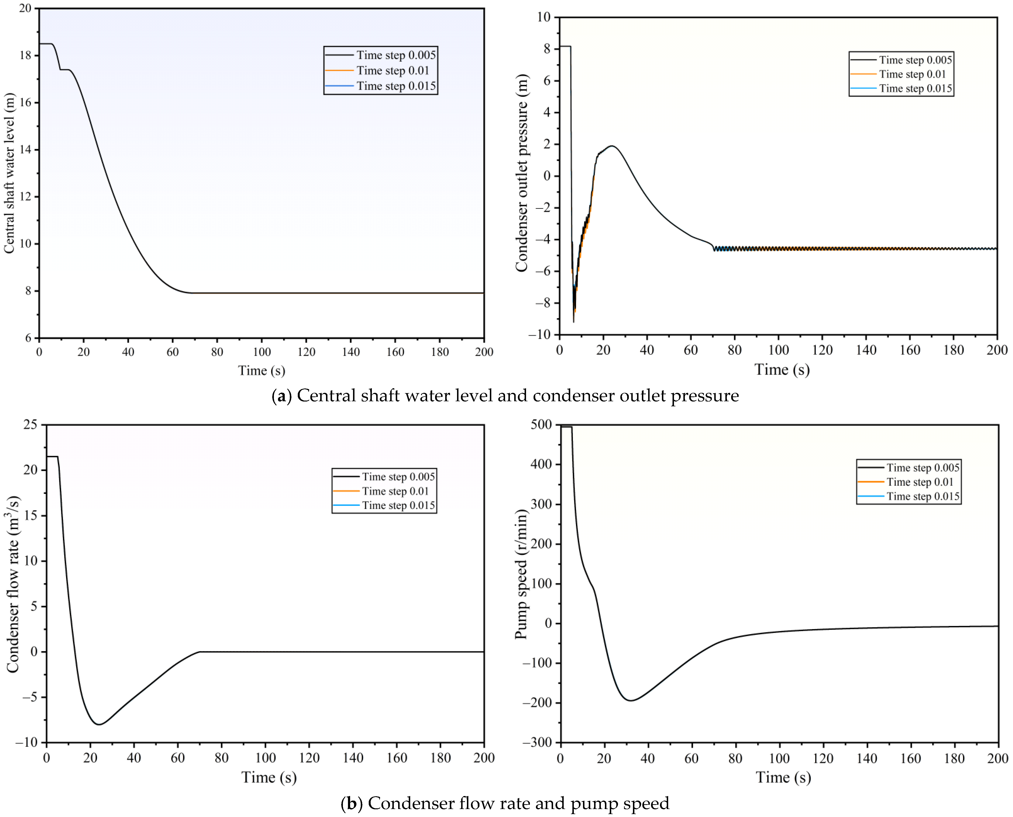
The time step is a key discrete parameter in numerical simulation, directly affecting the accuracy and stability of transient flow calculations in capturing water hammer wave propagation and pressure extrema. To verify the time step convergence of model C, the original time step was 0.01 s. This study selected two time step sets of 0.005 s and 0.015 s for sensitivity analysis, and the calculation results are shown below. The calculation results are shown in Figure 15 below.

As shown in

Table 8. Sensitivity analysis of time step in Model C.

Time Step (s)	Butterfly Valve Outlet Pressure (m)		Condenser Outlet Pressure (m)		Condenser Flow Rate (m3/s)	Water Pump Speed (r/min)	Central Shaft Water Level (m)	Along the Way (m)
	Maximum Value	Minimum Value	Maximum Value	Minimum value	Minimum Value	Minimum Value	Minimum Value	Maximum Value	Minimum Value
0.005	28.93	2.57	8.18	−9.21	−8.02	−194.46	7.92	30.48	−9.21
0.010	28.93	2.58	8.18	−9.16	−8.02	−194.47	7.91	30.48	−9.16
0.015	28.93	2.66	8.18	−8.43	−8.00	−194.45	7.90	30.47	−8.43

, the time step has a significant impact on the accuracy of the calculation results. When the time step increases from 0.005 s to 0.015 s, the minimum butterfly valve outlet pressure slightly increases from 2.57 m to 2.66 m; the minimum condenser outlet pressure increases significantly from −9.21 m to −8.43 m, and the negative pressure extreme value is underestimated by about 0.78 m; the minimum friction head correspondingly changes from −9.21 m to −8.43 m. In contrast, the extreme value of the pump reverse speed remains stable between −194.45 r/min and −194.47 r/min, the minimum condenser flow rate remains in the range of −8.00 m³/s to −8.02 m³/s, and the lowest water level in the central shaft only slightly decreases from 7.92 m to 7.90 m. The above results indicate that an excessively large time step (0.015 s) weakens the ability to capture the peak value of water hammer negative pressure due to increased discretization error, leading to a significant underestimation of the condenser outlet negative pressure. However, the impact of the time step is relatively small for variables such as rotational speed, flow rate, and water level. When the time step is further reduced from 0.01 s to 0.005 s, the variation range of each hydraulic parameter becomes very limited (the minimum condenser outlet pressure differs by only 0.05 m), indicating that the calculation results have basically converged when the time step is less than or equal to 0.01 s. Considering both computational efficiency and accuracy requirements, this study recommends using 0.01 s as the baseline time step for model C. This value can effectively control the computation time while ensuring acceptable accuracy in engineering applications.

In summary, model C exhibits good numerical stability within the time step range of 0.005 s to 0.01 s. However, it should be noted that an excessively large time step may lead to a non-conservative estimate of the extreme value of negative pressure. In practical engineering applications, it is recommended to use a time step of 0.01 s for transient flow simulation.

6. Conclusions

This paper constructs four equivalent models of the central shaft of the cooling tower for the simultaneous power outage of four circulating water pumps, and uses the method of characteristics to simulate the hydraulic transient process. Based on the numerical simulation results, the following conclusions are drawn:

(1)

Under the condition of pump shutdown, the hydraulic response of the circulating water system exhibits significant stage characteristics. After the pumps stop, the pump speed drops rapidly, reaching zero and reversing within 10–20 s; the water flow in the pipes reverses within 12–14 s. The minimum pressure head at the condenser outlet is close to −9 m, indicating a significant risk of negative pressure, which should be carefully prevented.

(2)

The equivalent modeling method of the shaft significantly affects the calculation results. Model A (fixed water level) gives the system unlimited water replenishment capacity, with the maximum reverse speed and reverse flow rate, resulting in a conservative approach. It can be used as an upper limit reference for safety verification, but it cannot reflect the dynamic adjustment effect of water level. Model B (considering water level changes but ignoring the high-level outflow of the distribution tank) leads to a larger drop in the shaft water level, resulting in a systematic bias. Model D (which splits the shaft into an equivalent pipe and a surge tank) overestimates the storage capacity and sets the lowest water level (13.30 m) too high, potentially underestimating hydraulic risks.

(3)

Model C has the best overall simulation accuracy and is recommended for similar projects. This model fully describes the physical process of water entering from the bottom of the shaft, flowing out through the distribution channel at the corresponding height, and accurately captures the dynamic characteristics of the water level dropping to the distribution channel elevation, maintaining a low level briefly, and then continuing to drop. Its minimum pressure envelope along the flow path is consistent with that of Model B, and its simulation of negative pressure extreme values is more reasonable. It achieves a good balance between accuracy, physical rationality, and engineering applicability, providing a reliable basis for water hammer protection design.

References

1. Wang, X.; Wu, J.C.; Piao, L. Consideration of the development situation of nuclear power under the goal of carbon peaking and carbon neutraulity. Nucl. Sci. Eng. 2022, 42, 241–245. [Google Scholar]
2. Zou, C.; Gong, M.J.; Chen, Y.F.; Zhang, Y.H.; Jiang, H.L. The simulation study of the startup process characteristics of the condenser in the secondary loop system of nuclear power plant. Nucl. Sci. Eng. 2022, 42, 707–715. [Google Scholar]
3. Niu, H.S.; Yang, R.B.; Lu, C.; Li, J. Comparison and selection of direct cooling and secondary cooling schemes for circulating water system of a coastal nuclear power plant. Water Wastewater Eng. 2018, 54, 1–4. [Google Scholar]
4. Wu, Q.W.; Qi, W.M. Stable and transient phenomena of circulating water system in nuclear power station. China Water Wastewater 2013, 29, 96–98. [Google Scholar]
5. Gao, G.; Wang, S.X. Study on the state control of important system in secondary circuit of nuclear power station after loss of off-site AC power supply. Electr. Technol. 2023, 24, 74–78. [Google Scholar]
6. Sharifullin, V.N.; Badriev, A.I. Aerodynamic characteristics of the cooling tower under the nonuniform distribution of the water and air flows. Therm. Eng. 2019, 66, 569–574. [Google Scholar] [CrossRef]
7. Bai, Y.C.; Liu, J.Y.; Yang, S.Q. Numerical simulation on hydraulic transient process of cooling water system in thermal power plant. Water Resour. Hydropower Eng. 2011, 42, 25–28. [Google Scholar]
8. Wang, X.H.; Fan, Y.Z.; Chen, G. Transient analysis of the circulating water system of nuclear power plant and selection of siphon break valve. Nucl. Sci. Eng. 2010, 30, 217–223. [Google Scholar]
9. Chapman, R.L.; Christensen, D.D.; Dafoe, R.E.; Hanner, O.M.; Wells, M.E. Compilation of Data Concerning Known and Suspected Water Hammer Events in Nuclear Power Plants: CY 1969; NUREG/CR-2059; EG&G Idaho, Inc.: Idaho Falls, ID, USA, 1981. [Google Scholar]
10. Chen, M.F. Analysis of water hammer phenomenon in industrial pipelines. Constr. Sci. Technol. 2004, 53. [Google Scholar] [CrossRef]
11. Liu, Z.Y.; Liu, G.L.; Su, F.J. Numerical simulation of pump-stopping water hammer in tertiary circulating water system of PWR nuclear power plant. Nucl. Power Eng. 2005, 26, 502–505. [Google Scholar]
12. Lu, C.; Yang, J.; Zhang, Q. Pressure Transient Analysis on the Condenser of the HPR1000 Nuclear Power Unit. Energies 2024, 17, 1210. [Google Scholar] [CrossRef]
13. Yang, C.; Zhang, Q.; Lu, C.; Huang, S.; Zhang, T.; Zhang, Z. Numerical simulation of typical abnormal operating conditions in the secondary circuit system of a Hua-long Pressurized Reactor nuclear power unit. Ann. Nucl. Energy 2024, 201, 110406. [Google Scholar] [CrossRef]
14. Gong, M.; Peng, M.; Zhu, H. Research of parameter distributing simulation and modeling for the condenser in nuclear power plant. Ann. Nucl. Energy 2019, 133, 313–326. [Google Scholar] [CrossRef]
15. Liu, W.X.; Tan, P.; Yang, J.G. Study on two-stage closure of valve stroking for water hammer protection of unexpected pump-stop. Fluid Mach. 2020, 48, 53–57. [Google Scholar]
16. Liu, Z.; Li, J.; Gui, B.; Li, X.Y.; Zhao, K. Research on the hydraulic transition process of circulating water system of cooling tower with high-level water collecting devices. Hebei Electr. Power 2021, 40, 38–41. [Google Scholar]
17. Zeng, H.; Yang, Z.Y.; Wu, L.Z.; Liao, N.P. Research of hydraulic transients for circulating water system with cooling tower with water collecting devices. Electr. Power Surv. Des. 2017, 310–314. [Google Scholar] [CrossRef]
18. Wang, Y.; Luo, L.Y.; Xu, S.K.; Zhao, J.X. Two stage valve closing protection for condenser water hammer of circulating water system in power plant. Water Technol. 2022, 16, 19–23. [Google Scholar]
19. Wang, F.; Feng, G.Y.; Zhang, R.Y.; Bai, W. Calculation and study of hydraulic transient flow in once-through circulating water system. Water Wastewater Eng. 2018, 54, 48–53. [Google Scholar]
20. Huang, B.; Zhang, X.A.; Wu, W.Q.; Zhang, L.Q.; Zeng, X.K.; Wang, T.; Zan, Y.F. Optimization study on winter operating procedures of circulating water system of a 1000 MW PWR nuclear power plant. Electr. Eng. 2023, 244–247. [Google Scholar] [CrossRef]
21. Wang, Y.; Zhao, Y.J.; Ding, W.H.; Zhao, J.X.; Xu, S.K.; Luo, L.Y.; Wang, W.K. The numerical modeling of water hammer to siphon well at cooling water system of thermal power station. Water Sci. Eng. Technol. 2022, 85–87. [Google Scholar] [CrossRef]
22. Jiao, Y.L.; Zheng, C.; Xu, T.; Yang, S.; Peng, C. Study on energy saving optimization of circulating water system in nuclear power plant based on Flowmaster simulation. J. Shanghai Univ. Electr. Power 2022, 38, 557–562. [Google Scholar]
23. Huang, Q.; Zhi, Y.; Zhang, R.; Du, X.; Zhang, J.; Wang, J. Flow Heat Transfer Characteristics and Dynamic Response of Once-Through Cooling Water System in Nuclear Power Plants Under Complex Operating Conditions. Energies 2025, 18, 1207. [Google Scholar] [CrossRef]
24. Wang, X.H.; Xiong, X.C.; Xue, H.Q. Water hammer calculation and prevention of auxiliary cooling water system in nuclear power plant. Power Syst. Clean Energy 2014, 30, 102–105. [Google Scholar]
25. Li, M.; Sun, P.; Wei, X. Optimal design of circulating water system in pressurized water reactor nuclear power plant. Ann. Nucl. Energy 2024, 207, 110751. [Google Scholar] [CrossRef]
26. Zhao, S.L.; Zhou, C.G. Design of circulating water pipeline in coastal nuclear power plant. Water Wastewater Eng. 2016, 52, 13–16. [Google Scholar]
27. Wylie, E.B.; Streeter, V.L. Fluid Transients; McGraw-Hill International Book Co.: New York, NY, USA, 1978. [Google Scholar]
28. Xie, J.; Huang, W.; Li, H.K.; Lin, H.K.; Wan, Z.H.; Zeng, M. Study on hydraulic control of combined valve group in long-distance gravity flow water delivery system. Water Wastewater Eng. 2023, 59, 104–112. [Google Scholar]
29. Luo, C.C.; Zheng, J.W. Calculation and study on protective measures for negative water hammer of condensers in thermal power plant. Electr. Power Surv. Des. 2022, 12–17. [Google Scholar] [CrossRef]
30. Huang, G.H.; Tang, S.W. Research on water hammer protection of circulating water system in thermal power plant based on orthogonal experiment method. Jiangxi Electr. Power 2019, 43, 49–51. [Google Scholar]
31. Wang, Z. Analysis of the Hydraulic Transient in Water-Cooling System of Power Plants. Master’s Thesis, North China Electric Power University, Baoding, China, 2008. [Google Scholar]
32. State Key Laboratory of Hydraulics and Mountain River Engineering, Sichuan University. Hydraulics, 5th ed.; Higher Education Press: Beijing, China, 2016; Volume 1. [Google Scholar]
Figure 1. Schematic diagram of the circulating cooling water system.
Energies 19 02400 g001
Figure 2. Schematic diagram of a bidirectional surge tank.
Energies 19 02400 g002
Figure 3. Schematic diagram of a two-branch water tower.
Energies 19 02400 g003
Figure 4. Schematic diagram of a partially submerged circular pipe.
Energies 19 02400 g004
Figure 5. Simplified diagram of circulating cooling water system.
Energies 19 02400 g005
Figure 6. Calculated results of hydraulic transients for Model A.
Energies 19 02400 g006
Figure 7. Calculated results of hydraulic transients for Model B.
Energies 19 02400 g007
Figure 8. Calculated results of hydraulic transients for Model C.
Energies 19 02400 g008
Figure 9. Calculated results of hydraulic transients for Model D.
Energies 19 02400 g009
Figure 10. Pressure head envelopes along the pipeline for the four models.
Energies 19 02400 g010
Figure 11. Comparison of hydraulic characteristics of four models over time.
Energies 19 02400 g011aEnergies 19 02400 g011b
Figure 12. Comparison results of sensitivity analysis of water pump rotational inertia.
Energies 19 02400 g012aEnergies 19 02400 g012b
Figure 13. Comparison results of sensitivity analysis of pipe roughness.
Energies 19 02400 g013
Figure 14. Comparison results of sensitivity analysis of Shaft cross-sectional area.
Energies 19 02400 g014aEnergies 19 02400 g014b
Figure 15. Comparison results of sensitivity analysis of time step.
Energies 19 02400 g015