Article

Large-Eddy Simulation of an Extended Wind Farm Using PALM Model System: Wake Dynamics and Power Output

by
Mohamed H. Salim
1,2,*,
Mohamed A. Mohamed
3,4,
Mohamed F. C. Esmail
1 and
Ibrahim K. Mohamed
1,5
1
Faculty of Energy Engineering, Aswan University, Aswan 81528, Egypt
2
Institute of Ecology, Technische Universität Berlin, 10587 Berlin, Germany
3
Faculty of Engineering, South Valley University, Qena 83523, Egypt
4
Aerospace and Mechanical Engineering Department, University of South Wales, Pontypridd CF37 1DL, UK
5
Faculty of Engineering, King Abdulaziz University, Rabigh 25732, Saudi Arabia
*
Author to whom correspondence should be addressed.
Energies 2026, 19(10), 2391; https://doi.org/10.3390/en19102391
Submission received: 8 April 2026 / Revised: 7 May 2026 / Accepted: 14 May 2026 / Published: 16 May 2026

Abstract

Large-eddy simulation (LES) of wind farms is often limited by the computational cost required to represent many turbine rows and to obtain statistically converged wake and power statistics. Here, we present LES of an extended wind-farm configuration using the PALM model system, where cyclic lateral boundary conditions are employed to emulate interior-farm interaction in an idealized neutral boundary layer. The setup consists of nine identical horizontal-axis wind turbines arranged in a staggered array within the computational domain. Time-averaged hub-height fields show coherent wake corridors with a mean inflow-speed reduction of 23.7 % (array-mean across turbines) relative to an undisturbed background wind speed, and peak wake deficits reaching 71.4 % in the near-wake region. Turbulence levels increase markedly in the wake shear layers, with hub-height turbulence intensity enhanced by 32.2 % in the rotor region compared to background conditions; correspondingly, the peak hub-height SGS-TKE increases by a factor of 6.74 relative to background. Vertically averaged profiles indicate a momentum deficit within the turbine layer and gradual recovery aloft; the streamwise turbulent momentum flux remains predominantly negative, demonstrating the downward transport of higher-momentum air from above as a key recovery mechanism. Turbine rotor-power statistics show an initial adjustment followed by a quasi-stationary regime, with a farm-mean rotor power of 1.93 MW and persistent inter-turbine variability characterized by a mean coefficient of variation of 61.2 %. Overall, the results demonstrate that the proposed extended-farm LES approach enables computationally efficient quantification of wake dynamics, vertical momentum transport, and their impact on power variability under idealized neutral wind-farm conditions.

1. Introduction

Wind energy has become a central source of the global transition toward low-carbon electricity. As installed capacity continues to grow, wind farms are increasingly deployed as large clusters, and their performance is determined not only by individual turbine characteristics but also by complex flow interactions at the array and farm scales [1,2]. A defining feature of wind farms is the formation of turbine wakes—regions of reduced mean wind speed and enhanced turbulence—whose interaction can significantly reduce downstream power production and increase structural loading [3,4]. Accurately representing wake evolution and wake–wake interaction is therefore essential for the reliable prediction of energy yield, power variability, and the aerodynamic environment experienced by turbines across the farm.
A wide range of modeling tools is available to study wind-farm aerodynamics, ranging from engineering wake models to computational fluid dynamics approaches such as Reynolds-averaged Navier–Stokes (RANS) [5,6], hybrid RANS-LES [7,8], and large-eddy simulation (LES) [9,10,11]. Engineering models offer rapid estimates and are widely used in design and optimization but typically rely on parameterizations for wake expansion, turbulence growth, and wake superposition that may not fully capture unsteady wake meandering, coherent turbulence structures, and the detailed coupling between atmospheric turbulence and turbine-induced flow. RANS approaches provide additional flow-field information at moderate computational cost but may struggle to represent the inherently unsteady, three-dimensional turbulence that strongly influences wake recovery and turbine-to-turbine interaction [5,6]. In contrast, LES resolves the large energy-containing turbulent eddies and has proven particularly valuable for wind-farm studies, as it can reproduce key mechanisms such as wake meandering, turbulence intensification in the wake, and the modulation of wakes by atmospheric boundary-layer (ABL) turbulence. LES thus provides a physically grounded pathway to connect wind-farm flow dynamics to turbine-level and farm-level power outputs [12].
Recent wind-farm research has advanced across multiple modeling levels. Engineering wake models have been extended beyond classical top-hat and superposition concepts to incorporate wake deflection, turbulence-added mixing, and stability dependence, enabling improved farm-level optimization at low computational cost [2,13,14]. At the CFD level, RANS-based actuator-disk and actuator-line frameworks remain widely used for layout and performance assessment, with ongoing progress in turbulence closures, rotor modeling, and inflow specification for atmospheric boundary-layer conditions [15,16,17]. Hybrid RANS-LES approaches have been increasingly applied to reduce cost while capturing unsteady wake meandering and partial turbulence spectra in multi-turbine configurations [18,19]. Nevertheless, wind-farm LES has matured into a reference tool for process understanding and benchmark-quality datasets, including studies on deep-array behavior, internal boundary-layer development, wake recovery mechanisms, and the role of atmospheric stability and surface forcing [20,21,22]. These developments provide the context for the present work to use LES to resolve wake dynamics and power variability, while explicitly addressing the computational constraints associated with extended-farm simulation. Salim Despite these advantages, LES of wind farms faces a persistent challenge: representing extended wind farms—farms with many turbine rows where flow statistics may evolve toward a quasi-equilibrium “extended-farm” regime—can be computationally demanding [23]. Simulating a large number of turbines requires large domains and long integration times to obtain statistically converged results, especially when the objective is to quantify not only mean wake deficits but also turbulence statistics and power variability [24]. Moreover, the flow in large wind farms may exhibit farm-scale features, including the development of an internal boundary layer and spatially heterogeneous turbulence production, which are difficult to infer from simulations that include only a few turbines or a limited number of rows [25]. As a consequence, many high-fidelity studies adopt limited arrays or focus on idealized configurations, while studies targeting extended-farm behavior often require substantial computational resources and the careful treatment of boundary conditions and inflow turbulence [26].
This work addresses the above challenge by presenting LES of an extended wind-farm configuration using the PALM model system [27], with an emphasis on wake dynamics and turbine power output. PALM is a high-performance LES framework designed for atmospheric boundary-layer flows and has been applied broadly in microscale meteorology and related applications [28], offering strong parallel scalability for computationally intensive turbulence-resolving simulations [29]. The methodological novelty of this study lies in combining PALM’s wind-turbine modeling capabilities with cyclic lateral boundary conditions to emulate sustained interior-farm interaction using a limited turbine subset. In contrast to conventional finite-farm LES that requires many turbine rows and large domains to approach extended-farm statistics, the cyclic configuration allows wake interactions to persist and recirculate, enabling longer effective interaction pathways and improved statistical sampling at substantially reduced computational cost. The concrete value of this approach is twofold: (i) it provides a practical route to quantify wake recovery mechanisms and power variability in an interior-farm-like regime without simulating the full spatial extent of a large wind farm, and (ii) it facilitates systematic sensitivity studies (e.g., spacing, yaw settings, and inflow conditions) by lowering the cost per experiment compared to deep-array simulations in large finite domains [30,31].
The scientific focus of the paper is twofold. First, we quantify the wind-field structure associated with wake formation, interaction, and recovery within the simulated farm, analyzing both mean flow modifications and turbulence-related features that govern wake evolution. This includes the spatial organization of velocity deficits, shear layers, and turbulence intensification in and around wakes, as well as the degree to which wake signatures persist across the turbine array. Second, we connect these flow features to turbine power output, examining how wake exposure and local turbulence influence power production across the array and how power statistics vary in space and time under extended-farm conditions. By combining flow-field diagnostics with turbine-level power time series, the study provides a consistent picture of how turbine–ABL interaction and wake–wake interaction shape energy extraction within a wind farm.
Accordingly, the objectives of this work are to characterize the spatial patterns of wake deficits and wake interaction in the farm, including hub-height flow modifications and indicators of wake recovery; to assess turbulence changes induced by turbines (e.g., turbulence intensification and redistribution) and discuss implications for wake persistence and mixing; to quantify turbine power output statistics (mean, variability, and spatial contrasts across the array) and relate them to local flow conditions; and to demonstrate that the adopted modeling setup can reproduce wind-farm-like interaction patterns that are characteristic of larger arrays, enabling the efficient investigation of extended-farm behavior.
The main contributions of this paper are therefore (i) a PALM-based LES configuration tailored to represent extended wind-farm conditions with a limited turbine subset, (ii) a comprehensive analysis of wake dynamics using resolved flow fields, and (iii) a turbine-level assessment of power output and its relation to wake exposure and turbulence conditions. These contributions aim to support both methodological development (efficient high-fidelity simulation strategies) and physical understanding of how wakes and turbulence control energy extraction in large wind farms.
The remainder of the paper is organized as follows. Section 2 describes the numerical methodology, including the PALM configuration, turbine representation, computational domain, boundary conditions, and diagnostics used for flow and power analysis. Section 3 presents the simulated wind-field results and wake characteristics, followed by an analysis of turbine power outputs and their spatial variability across the array. Section 4 discusses the implications, limitations, and potential extensions toward more complex atmospheric conditions and larger parameter spaces. Section 5 summarizes the main conclusions.

2. Materials and Methods

2.1. Domain Size and Wind-Turbines Data

The computational domain ( L x = 2300 m , L y = 2240 m , L z = 1650 m ) is discretized on a Cartesian grid with n x = 576 , n y = 560 , and n z = 256 . The vertical grid uses Δ z = 2 m near the surface and within the rotor region, with grid stretching above the stretching level z = 350 m , resulting in a model-top height of 1650 m. To facilitate comparison across turbine/farm scales, the domain size is also reported in dimensionless form using the turbine rotor diameter ( D = 126 m ) as L x = 18.25 , L y = 17.78 , L z = 13.10 .
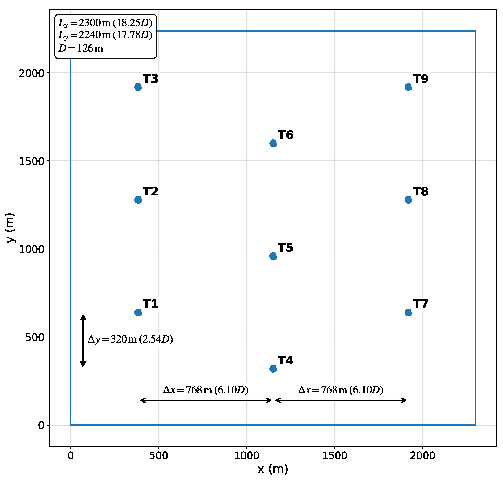
In the domain, a staggered configuration of 9 identical horizontal-axis wind turbines is represented ( n t = 9 ), as shown in Figure 1. Each turbine has hub height z h = 140 m , rotor radius R = 63 m (thus D = 2 R = 126 m ), tower diameter 4 m , and nacelle radius 1.5 m . The rated generator power is P rated = 5.3 MW . Initial yaw angles vary among turbines (Table 1), while speed, pitch, and yaw controls are enabled for all turbines. The yaw angles are prescribed initial conditions; therefore, lateral-flow and wake-deflection signatures are interpreted primarily as yaw-driven effects, whereas the extended-farm interpretation is based on streamwise deficit, momentum transport, and power statistics. A summary of the key turbine parameters is provided in Table 2.

2.2. PALM Model System and Wind Turbine Parameterization

The simulations were performed with the PALM model system (hereafter PALM), a turbulence-resolving large-eddy simulation (LES) framework for atmospheric and oceanic boundary-layer flows [27]. PALM discretizes the model domain on a Cartesian grid using finite differences with equidistant horizontal grid spacing and employs a two-dimensional domain decomposition in the horizontal directions to enable efficient parallelization.
PALM solves the three-dimensional filtered governing equations for momentum and scalars. By default, the prognostic variables comprise the velocity components ( u , v , w ) on a staggered Arakawa-C grid, potential temperature θ , subgrid-scale turbulent kinetic energy e (in LES mode), water vapor mixing ratio q v , and optionally a passive scalar. The governing equations are formulated as incompressible approximations of the Navier–Stokes equations, typically using a Boussinesq-approximated form (with an alternative anelastic option available for applications extending through a deeper tropospheric layer).
Turbulence effects smaller than the grid scale are represented via a subgrid-scale (SGS) closure. In LES mode, PALM employs a prognostic SGS-TKE (1.5-order) closure after Deardorff, with an additional dynamic SGS option available in PALM 6.0. Model output is written in netCDF format and PALM supports online statistics such as time and domain averaging to reduce the volume of stored data during computationally intensive LES runs. PALM has been evaluated in a wide range of boundary-layer applications, and validation studies are reported [27]. Within the PALM-4U development framework, dedicated observational and wind-tunnel datasets have been compiled to support one-to-one comparisons using PALM’s virtual-measurement concept, including large-scale evaluation efforts for real urban domains (e.g., Berlin, Hamburg, and Stuttgart).
The wind turbines are represented using the PALM wind turbine model (WTM), which is based on an advanced actuator disk approach including rotational effects (ADM-R). In contrast to a “classical” actuator disk model that prescribes a uniformly distributed thrust force only, the PALM-WTM accounts for both thrust and torque and resolves the radial (and tangential) variability of the loading based on a blade–element–momentum (BEM) formulation. This retains key wake characteristics (e.g., the ring-shaped near-wake structure) while remaining computationally efficient for multi-turbine LES since the time step is dictated by the flow solver rather than the rotor rotation.
Technically, the rotor disk is subdivided into annular segments (ring elements) whose size is linked to the grid spacing (default: 1 Δ in tangential and 0.5 Δ in radial direction). For each rotor segment, the local lift and drag forces per unit area are computed from the relative velocity U rel at the segment center and tabulated blade properties (chord and airfoil polars), i.e.,
f l = 1 2 ρ U rel 2 c l N b c 2 π r seg , f d = 1 2 ρ U rel 2 c d N b c 2 π r seg ,
where N b is the number of blades, c the local chord length, and r seg the radial distance of the segment from the rotor center. The relative velocity is formed from the local axial and tangential flow components and the blade segment speed Ω r seg , and the forces are projected onto the axial (thrust) and tangential (torque) directions:
f N = f l cos ϕ + f d sin ϕ , f Θ = f l sin ϕ + f d cos ϕ ,
with the inflow angle ϕ determined from the local axial and tangential velocities. The resulting forces are then interpolated to the LES grid and spatially smeared over a finite support around the rotor to avoid numerical artefacts; in PALM 6.0 this smearing is implemented efficiently using a polynomial kernel confined to the rotor vicinity (in earlier implementations a Gaussian kernel with a width of about two grid spacings was commonly used). The tower and nacelle are additionally represented through a drag-force approach using constant drag coefficients, and the combined rotor (thrust/torque) and tower/nacelle drag terms enter the momentum equations as sink/source terms.
The PALM-WTM includes baseline turbine control algorithms for wind-energy applications. A rotational speed controller and a collective pitch controller adjust the generator torque below and blade pitch above the rated conditions so that the electrical power follows the turbine power curve; power is computed from rotor torque and rotational speed with optional corrections for drivetrain efficiency. A yaw controller is also available to align the rotor with the incoming wind. The PALM-WTM has been applied in multiple wind-energy studies, including offshore wind-farm simulations investigating wake effects and stability impacts on power production. PALM and its wind-turbine modeling capabilities have been evaluated in previous studies and are documented in the PALM reference description and the wind-energy applications cited therein [27]. In the present work, we therefore focus on a process-level analysis of wake interaction and power variability in an idealized extended-farm configuration, rather than on site-specific validation against field or laboratory measurements.
For reproducibility, we note that the PALM wind turbine model (ADM-R) computes rotor loading from tabulated blade geometry and airfoil polars provided as input lookup tables [27]. In this study, these airfoil/polar tables and PALM’s built-in rotor-speed/pitch and yaw controllers were used as configured in the WTM setup following Maronga et al. [27].

2.3. Simulation and Numerical Setup

2.3.1. Numerical Setup

All simulations were performed with the PALM model system in large-eddy simulation (LES) mode, employing the incompressible, Boussinesq-approximated formulation on a staggered Arakawa C-grid [27]. For the spatial discretization, PALM uses finite differences with equidistant horizontal grid spacing, while the vertical grid can be stretched above the boundary-layer core to reduce computational cost without compromising near-rotor resolution [27]. Advection of momentum and scalar quantities was computed using the fifth-order Wicker–Skamarock scheme, and time integration employed a third-order Runge–Kutta scheme (RK3) [29]. Subgrid-scale (SGS) turbulent fluxes were represented with the 1.5-order TKE closure following the standard PALM LES configuration [27]. The perturbation pressure Poisson equation was solved with PALM’s multigrid solver to enforce mass conservation at each Runge–Kutta substep [27].

2.3.2. Computational Domain and Grid Resolution

The computational domain uses n x = 575 , n y = 559 , and n z = 256 grid points with uniform horizontal spacing Δ x = Δ y = 4 m, yielding physical extents of L x = ( n x + 1 ) Δ x = 2304 m and L y = ( n y + 1 ) Δ y = 2240 m. In the vertical direction, the near-surface and rotor-layer region is resolved with a uniform spacing Δ z = 2 m up to the stretching height z = 350 m. Above this level, the vertical grid is stretched using a factor of 1.04 up to a maximum spacing Δ z max = 60 m, resulting in a model-top height of approximately L z 1545 m. Relative to the rotor diameter ( D = 126 m), the domain size corresponds to L x / D = 18.29 , L y / D = 17.78 , and L z / D = 12.26 . A summary of the numerical setup is provided in Table 3.

2.3.3. Boundary Conditions and Near-Boundary Treatment

The wind-farm flow was driven by geostrophic forcing (prescribed geostrophic wind components) and a surface-layer treatment based on Monin–Obukhov similarity theory (MOST), consistent with the PALM core formulation for atmospheric boundary layers [27]. To emulate interior-farm interaction in an extended wind-farm environment, cyclic (periodic) boundary conditions were applied at all lateral boundaries in x and y, such that turbine wakes and turbulence structures leaving the domain re-enter from the opposite side [27]. This configuration eliminates conventional inflow/outflow boundary layers and reduces sensitivity to inflow specification, but it also implies that finite-farm edge effects are not represented; these limitations are discussed in Section 4. At the lower boundary, surface fluxes and stresses are applied through MOST. At the upper boundary, PALM applies a model-top treatment (commonly including a damping/sponge layer, depending on the configuration) to minimize spurious wave reflection and to ensure numerical stability [27]. Because lateral boundaries are periodic, the “near-boundary” flow at the sides is physically consistent with the interior solution; therefore, the main near-boundary considerations are associated with the surface layer and the model top rather than with inflow/outflow artefacts.

2.3.4. Initial Conditions, Spin-Up, and Averaging

The simulations assumed neutral stratification; accordingly, no prognostic potential-temperature equation was solved and a constant reference potential temperature was prescribed ( θ = 300 K). To trigger turbulence development and accelerate the formation of resolved eddies, the flow was initialized with small random perturbations within a specified height range (synthetic disturbances), following common practice in PALM-based ABL and wind-farm LES studies [29]. An initial spin-up phase of 3.5 h was discarded to allow the turbine–wake field and the turbulent flow to adjust within the periodic domain.
All statistics reported in Section 3 are computed over the subsequent post-spin-up (quasi-stationary) period, using consistent averaging windows across hub-height planes, vertical profiles/fluxes, and turbine power diagnostics. To demonstrate that the selected averaging period is sufficiently long for the main diagnostics, we provide a basic convergence assessment in Appendix A, where the cumulative averages of farm-mean rotor power and hub-height inflow-speed deficit are evaluated as a function of averaging time (Figure A1).

2.3.5. Grid-Sensitivity Analysis and Grid Convergence Index (GCI)

To assess the sensitivity of the predicted flow and turbine-response statistics to grid resolution, a mesh refinement study was performed following the Grid Convergence Index (GCI) procedures, e.g., [32,33,34,35]. Three systematically coarsened grids were considered while keeping the physical domain size and all model and turbine settings identical. The fine grid corresponds to the baseline configuration used throughout the main analysis, with Δ x = Δ y = 4 m and Δ z = 2 m in the rotor layer. Two coarser grids were then constructed as Coarse-1: Δ x = Δ y = 6 m , Δ z = 3 m , and Coarse-2: Δ x = Δ y = 8 m , Δ z = 4 m . For the vertical grid, the same stretching strategy and stretching height were retained across the three grids, while the near-surface/rotor-layer base spacing Δ z was adjusted according to the above refinement levels.
Following the GCI approach for three-dimensional simulations, a representative mesh size l was defined as
l = 1 N i = 1 N Δ v i 1 / 3 ,
where Δ v i is the volume of the ith grid cell and N is the total number of cells in the computational domain. A grid refinement factor was then computed from the ratio of representative mesh sizes between two grids, i.e., r = l fine / l coarse . For each target quantity ϕ (e.g., rotor power, hub-height velocity deficit, momentum flux, or turbulence metric), the relative error between two grids was evaluated as
ε = ϕ coarse ϕ fine ϕ fine ,
and an aggregate error measure was obtained from the root-mean-square value over a set of n representative samples (e.g., selected heights, turbine locations, or diagnostically relevant points) as
ε rms = i = 1 n ε i 2 n 1 / 2 .
In the present study, ε rms was evaluated in a consistent and reproducible manner for the selected target variables. For the hub-height velocity components (u, v, and w), ϕ denotes the time-mean field on the z = 140 m plane, interpolated to cell centers where required, and the RMS error in Equation (5) was computed over all horizontal grid points of that plane. For turbine power, ϕ denotes the turbine-mean rotor power for each turbine, and ε rms was computed over the set of turbine-mean values ( n = 9 ). This definition provides a domain-integrated measure of the sensitivity of the hub-height flow structure and a turbine-integrated measure of the sensitivity of the power response across the array.
Finally, the GCI for the fine-grid solution was computed as
GCI = F ε rms r p 1 ,
where p is the nominal order of accuracy of the spatial discretization and F is a safety factor. Consistent with common practice, F = 5 was used to provide a conservative estimate of numerical uncertainty. The resulting GCI values are reported for the key diagnostics used in the Results section, and the fine grid was retained for the main analysis based on the combined consideration of accuracy and computational cost.

3. Results

3.1. Grid-Sensitivity and GCI-Based Uncertainty Assessment

To quantify numerical uncertainty across the tested grids, we apply the GCI procedure described in Section 2.3.5. For each refinement step (Coarse-2 → Coarse-1 and Coarse-1 → Fine), we compute the RMS relative difference ε rms for representative diagnostics of the hub-height velocity components (u, v, and w) and for the turbine rotor power. Here, ε rms is evaluated over the selected sampling set (see Section 2.3.5), and the corresponding GCI provides a conservative estimate of the numerical uncertainty. The refinement ratio is defined as r = l fine / l coarse , where l is the representative mesh size based on the rotor-layer cell volume. Table 4 summarizes ε rms and GCI for each refinement step and target variable.
The grid-sensitivity analysis indicates that the main flow features are robust across the three tested resolutions. In particular, the hub-height velocity components reproduce the same wake-corridor structure and wake-interaction pattern, and regions of enhanced turbulence remain spatially co-located with wake shear layers. Differences between grids are most evident in quantities governed by sharp gradients in the rotor layer and near wake, where coarser meshes yield smoother wake edges and reduced peak values, while preserving the bulk wake deficit and the large-scale wake footprint.
Quantitatively, numerical sensitivity using the GCI procedure showed that the corresponding GCI values (Table 4) fall within 1.6–6.4%, indicating limited sensitivity of the hub-height velocity field and the turbine power statistics to grid spacing within the tested range. Based on these results, the fine grid was retained for the main analysis, as it provides the best compromise between accuracy and computational cost, while the reported GCI values provide conservative uncertainty bounds for the principal diagnostics discussed in the remainder of Section 3.

3.2. Hub-Height Flow Field and Wake Footprints

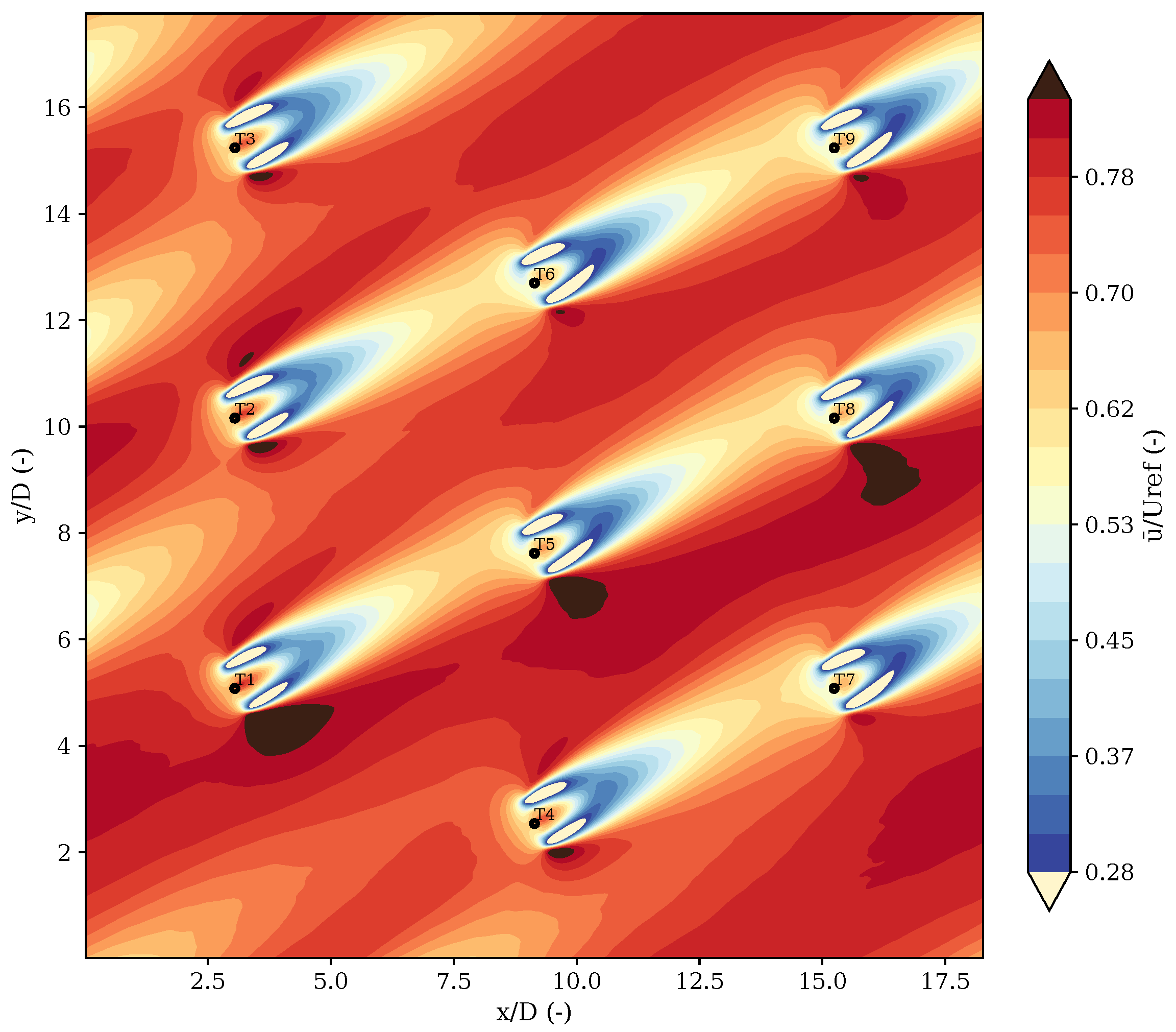
At the rotor-center height ( z = 140 m), the horizontally averaged streamwise velocity field reveals pronounced wake deficits downstream of each turbine location (Figure 2). The normalized mean u ¯ / U ref shows coherent wake cores with minimum values in the near wake and a gradual recovery with distance. Wake footprints are elongated and tilted diagonally across the domain, consistent with the combined action of the mean flow and the turbine-array arrangement. The spatial extent of the velocity deficit regions indicates that wake interactions are not confined to immediate downstream neighbors; rather, deficit regions extend over several rotor diameters and partially overlap with the downstream turbines’ inflow regions, implying systematic array-scale wake coupling.
To quantify the magnitude of the wake-induced inflow reduction, we sampled the hub-height wind-speed magnitude at the turbine locations and compared it to an undisturbed upstream reference speed U 0 diagnosed from a background region outside the turbine influence. Averaged across all turbines, the mean inflow speed is reduced by 23.72 % relative to U 0 , while the strongest near-wake deficit reaches 71.40 % (minimum hub-height speed within 1 8 D downstream of a turbine).
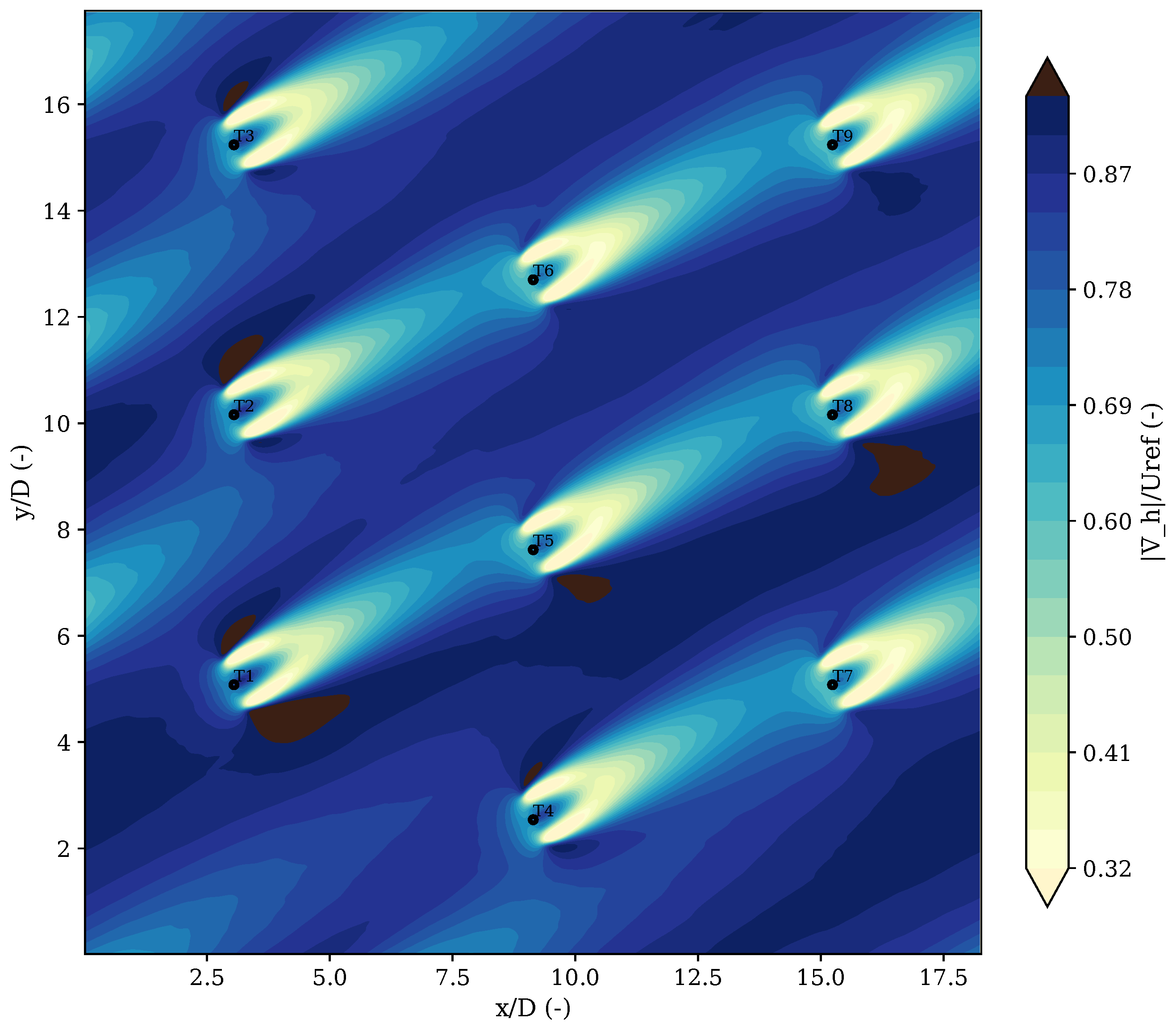
The plan-view wind-speed magnitude at hub height (Figure 3) complements the u ¯ / U ref field by highlighting the integrated impact of both streamwise deficits and lateral/vertical velocity contributions on the local inflow speed experienced by turbines. The normalized hub-height speed, | V ¯ h | / U ref , exhibits extended low-speed corridors aligned with the wake directions. In these regions, the local speed drops substantially relative to the reference value, demonstrating that the wake-induced reduction in kinetic energy persists over appreciable distances and contributes directly to reduced turbine inflow conditions in portions of the array.
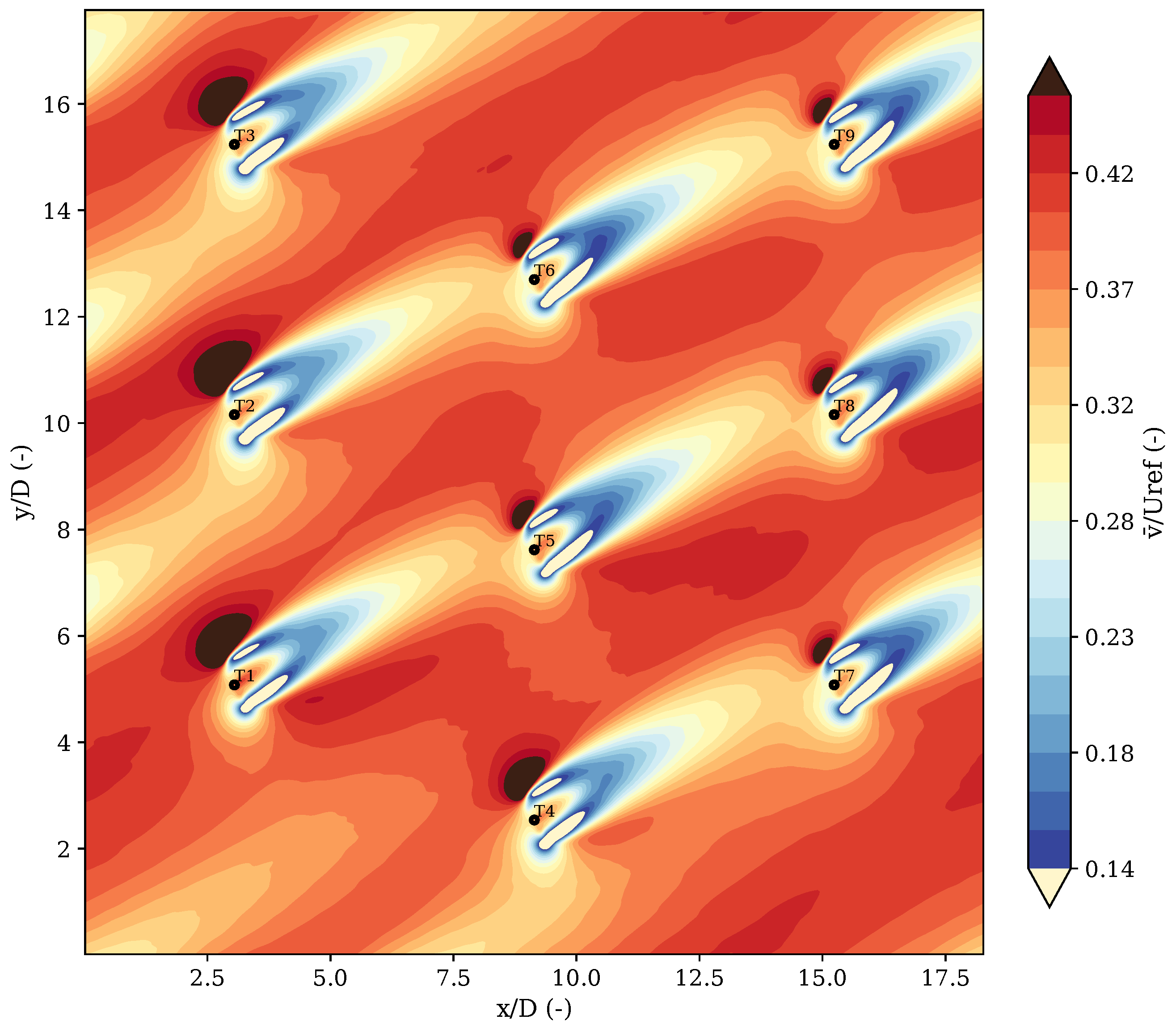
The lateral velocity component v ¯ / U ref exhibits a characteristic dipole-like structure around the turbine positions and within the wake regions (Figure 4). This pattern is consistent with wake deflection and cross-stream flow adjustment in response to turbine-induced forcing and yaw misalignment. Notably, the sign and strength of v ¯ / U ref vary across turbines, reflecting the prescribed yaw-angle distribution and the resulting asymmetric wake steering. The lateral velocity anomalies persist within the wake footprints and contribute to a gradual lateral redistribution of momentum at the array scale, which can modify the effective alignment of downstream wake impingement. In the following, lateral-flow and wake-deflection signatures are interpreted primarily as yaw-driven effects, whereas the extended-farm interpretation is based on streamwise deficit, momentum transport, and power statistics.
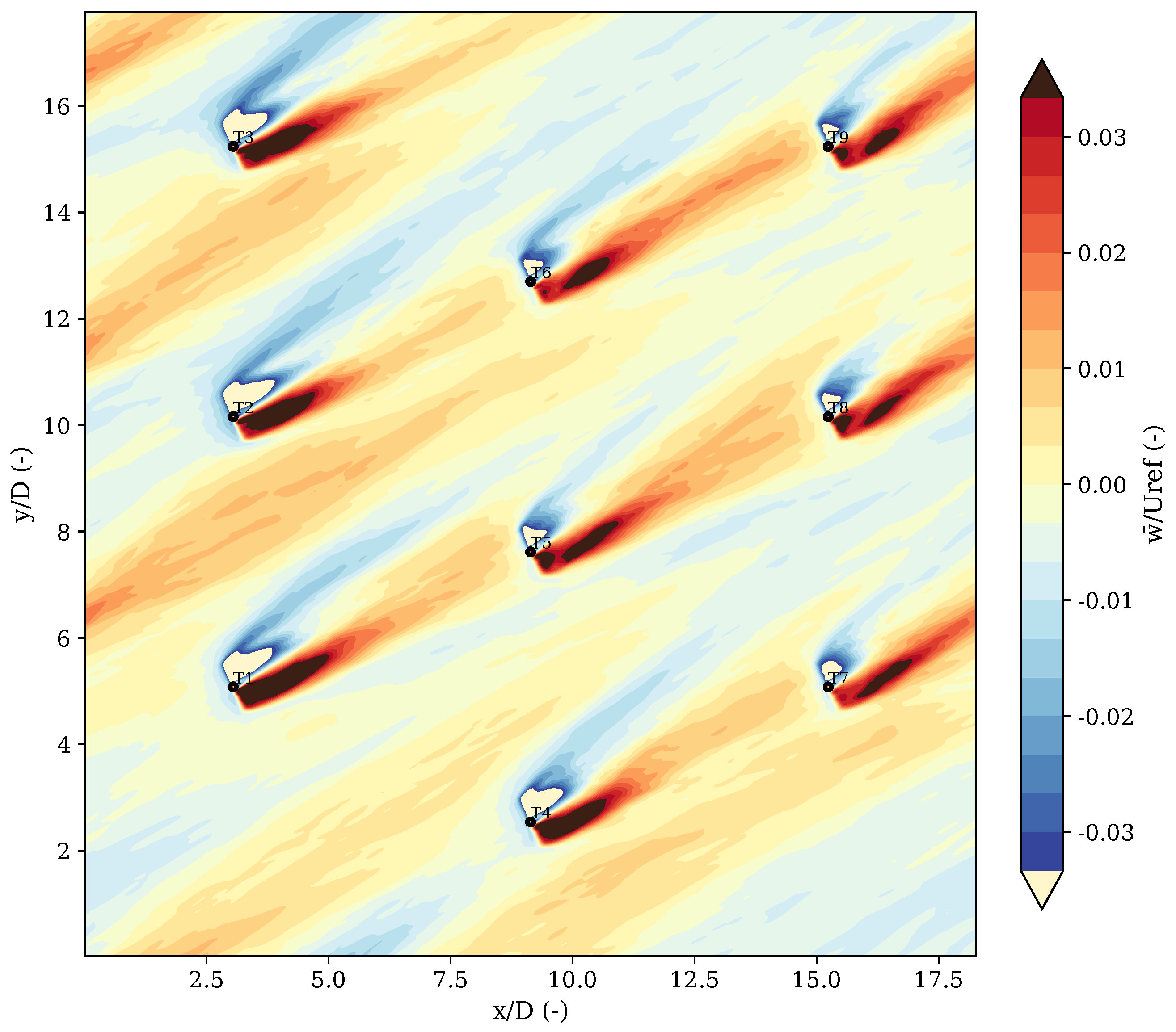
The vertical velocity field w ¯ / U ref displays localized updraft–downdraft pairs near turbines and in the near-wake region (Figure 5). These vertical motions are indicative of rotor-induced vertical momentum transport and wake-associated secondary circulations. Although the magnitude of w ¯ / U ref is small compared to u ¯ / U ref , the coherent vertical structures extend downstream and are spatially correlated with regions of strong shear at wake edges, implying an important role in turbulent mixing and wake recovery.
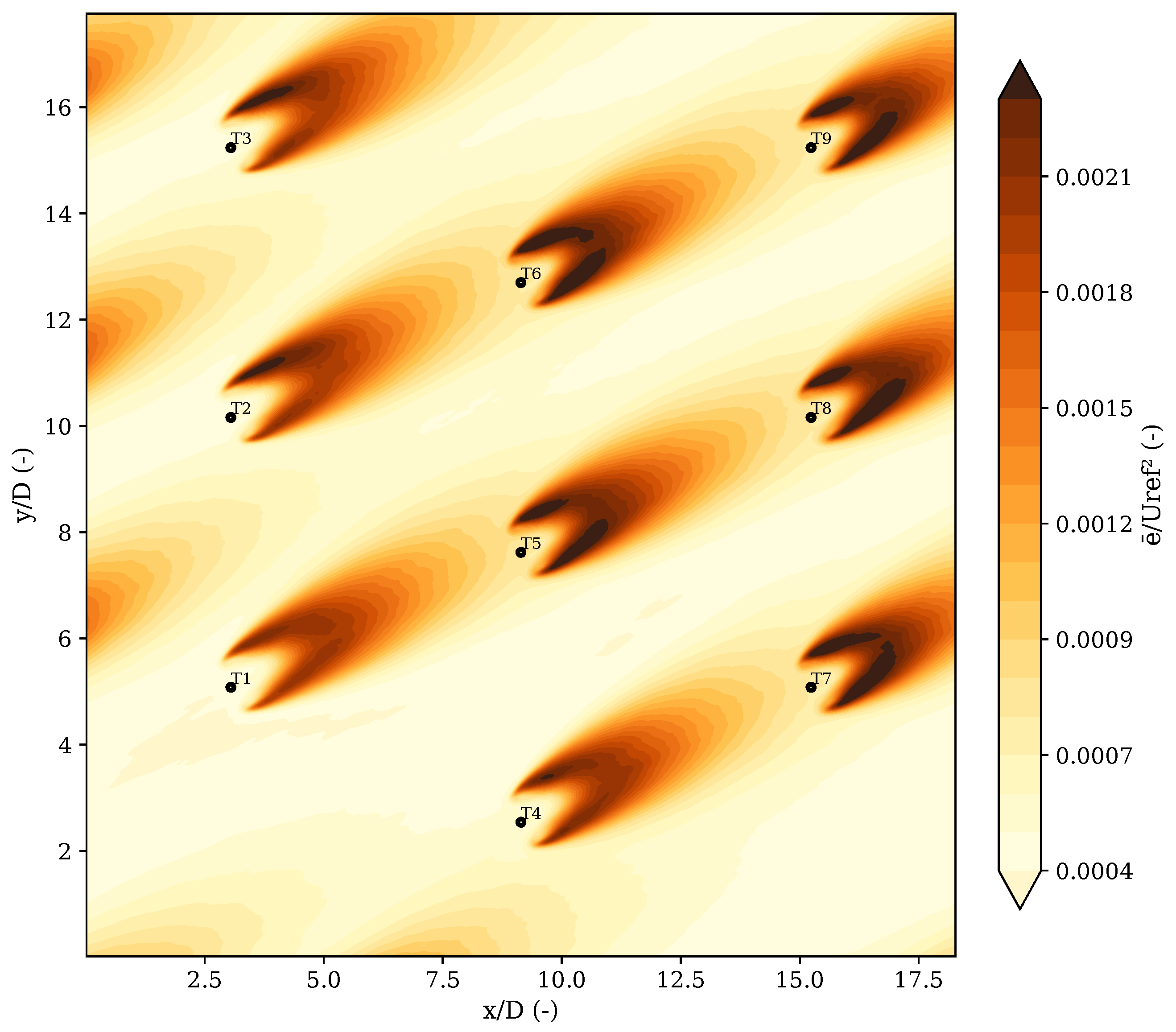
Enhanced turbulence levels are evident in the distribution of normalized subgrid-scale turbulent kinetic energy, e ¯ / U ref 2 (Figure 6). Peak e ¯ / U ref 2 values occur within and around the wake shear layers, particularly in the near-to-intermediate wake where velocity gradients are strongest. The elevated SGS-TKE footprints follow the wake paths and broaden downstream, consistent with progressive entrainment and mixing. This spatial co-location of strong velocity deficits (Figure 2) and elevated SGS-TKE (Figure 6) indicates that wake recovery in the array is governed by the balance between persistent momentum deficits and turbulence-enhanced mixing, with implications for downstream inflow quality and turbine power variability discussed later. Consistently, the peak rotor-layer SGS-TKE increases by 32.21 % relative to the background level, confirming that wake shear layers are the dominant regions of turbulence production in the turbine layer.
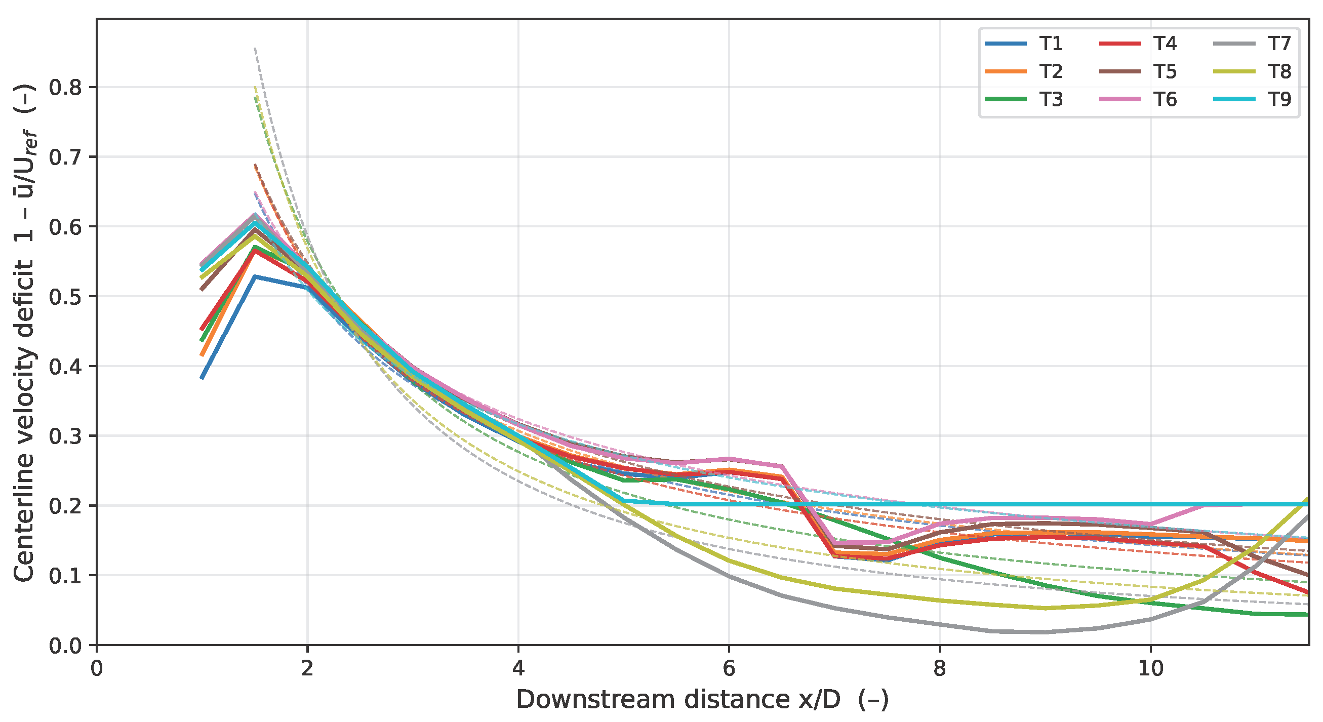
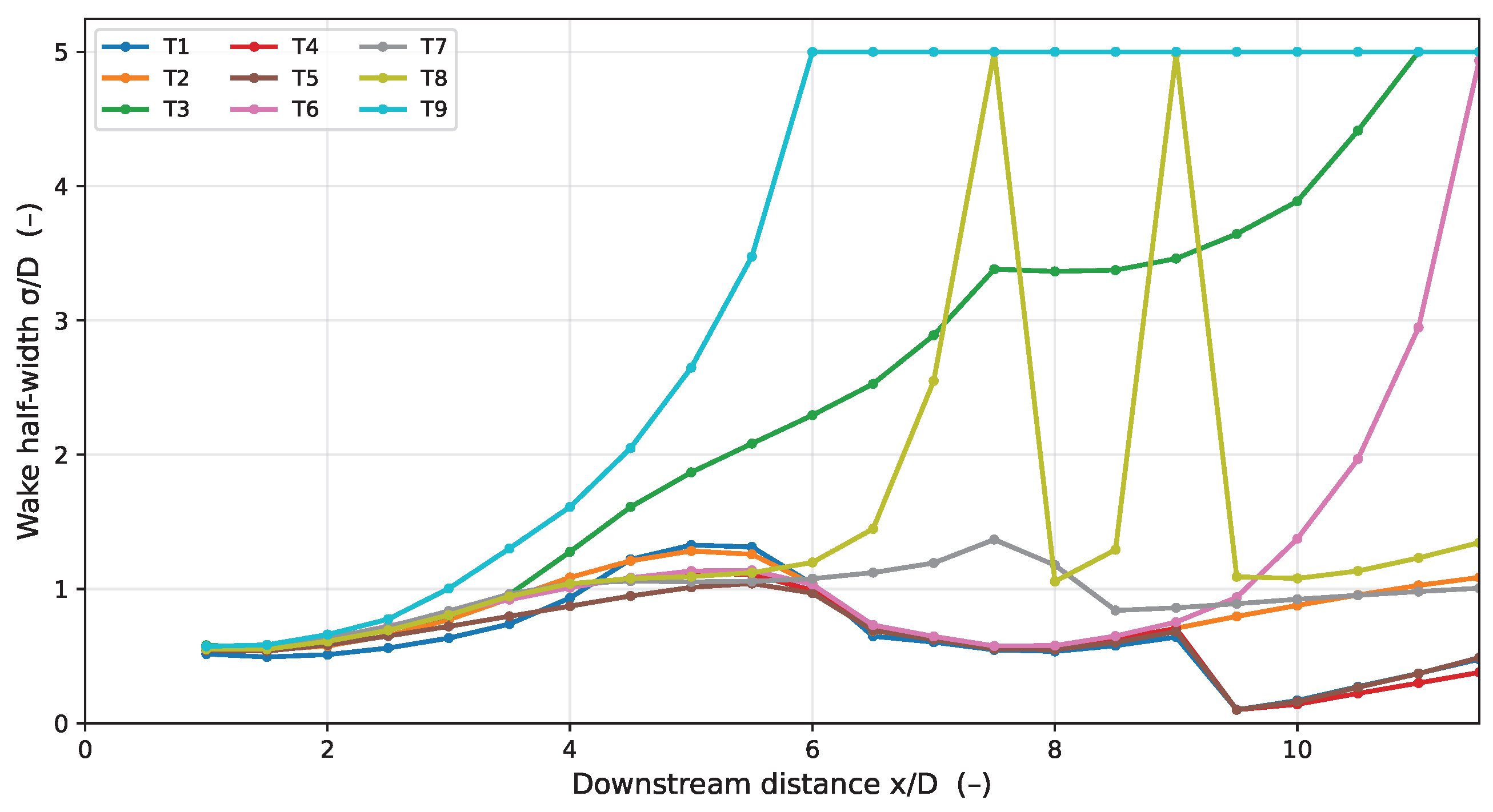
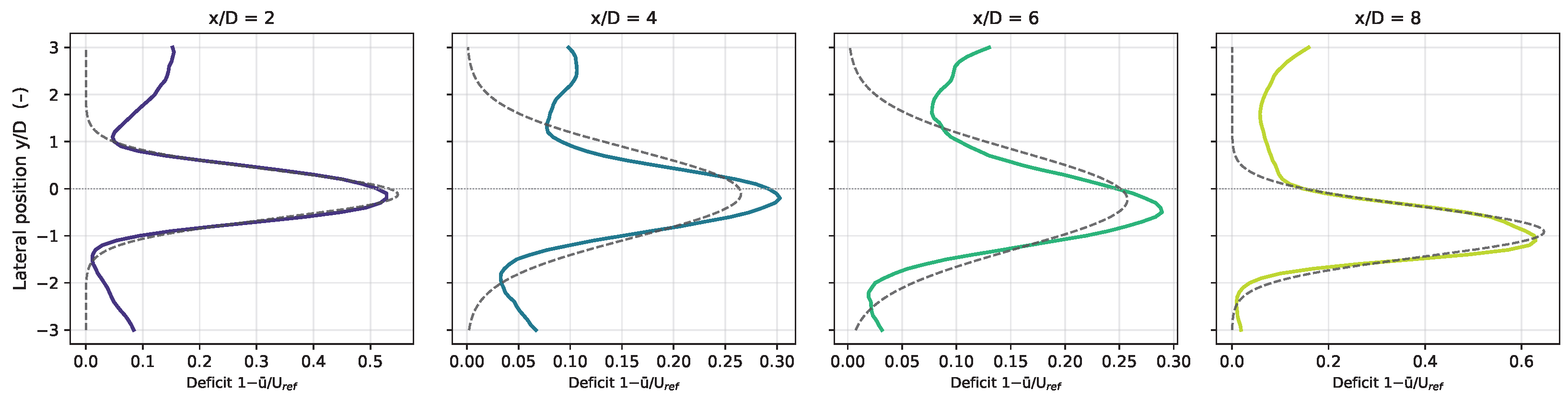
To complement the qualitative observations above, quantitative wake metrics were extracted from the time-averaged hub-height velocity field for all nine turbines and are reported in full in Appendix B. Centerline velocity deficits were sampled along the inflow-parallel wake axis from 1 D to 12 D downstream of each rotor and fitted with a power-law decay model Δ u ¯ / U ref = A ( x / D ) k (Figure A2). The fitted decay exponents range from k = 0.68 (T9) to k = 1.32 (T7), reflecting the strong influence of turbine position within the array on far-wake recovery. Front-row turbines (T1–T3) receive between 68% and 72% of U ref at the rotor disk, while interior turbines (T5, T6) experience inflows as low as 0.608 U ref , a reduction of approximately 15% relative to the undisturbed inflow. Gaussian fits to the lateral deficit profiles (Figure A4) confirm that wake half-widths grow monotonically with downstream distance for unobstructed wakes, reaching σ / D 1.3 at 5 D for T1. The persistence of deficits greater than 5% of U ref beyond 12 D for seven of the nine turbines (Table A1) demonstrates that the inter-turbine spacing is insufficient for full wake recovery, with direct implications for the power losses of downstream rows.

3.3. Vertical Structure of Mean Flow, Turbulence, and Momentum Fluxes

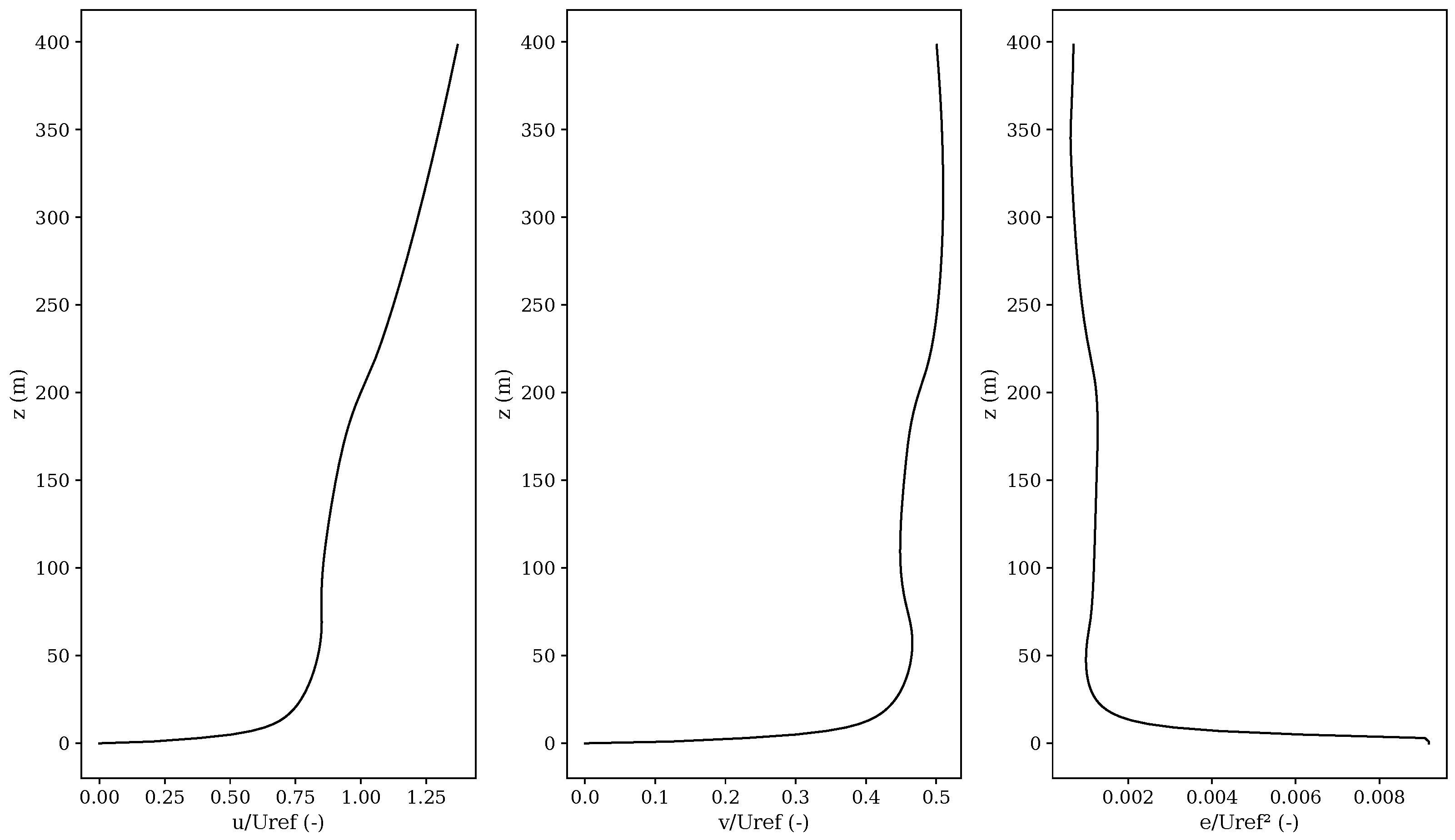
The vertically averaged profiles provide a compact view of how the turbine array modifies the mean flow and turbulence structure across the lower atmosphere (Figure 7). The normalized mean streamwise velocity profile, u ¯ / U ref , shows a pronounced velocity reduction within and above the rotor layer, with the largest deviation occurring around hub height ( z 140 m), consistent with momentum extraction by the turbines. Above the rotor region, u ¯ / U ref recovers gradually with height, indicating progressive replenishment of momentum from aloft through turbulent transport.
The corresponding profile of the normalized lateral velocity component, v ¯ / U ref , indicates a non-zero cross-stream mean flow over a broad vertical range (Figure 7). This reflects the combined impact of the prescribed yaw settings and wake-induced secondary motions, which introduce persistent lateral flow components and contribute to lateral redistribution of momentum in the array.
Turbulence levels, quantified here by the normalized subgrid-scale turbulent kinetic energy e ¯ / U ref 2 , are enhanced throughout the rotor layer and remain elevated up to several hundred meters as shown in Figure 7. The vertical structure suggests that turbine-induced shear production and mixing are not confined to the immediate rotor swept area but influence a deeper layer of the boundary layer, consistent with the broadened wake footprints observed at hub height.
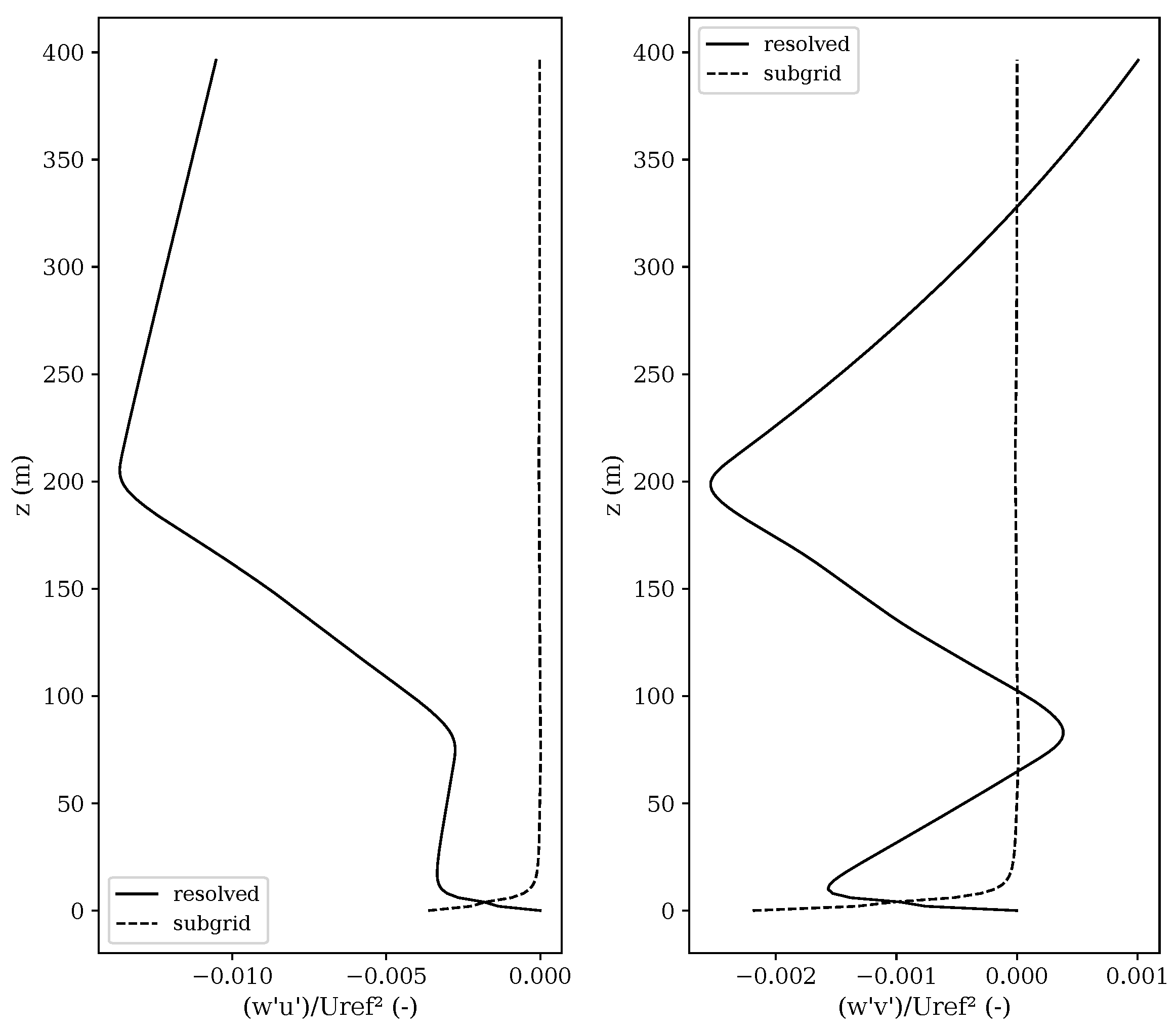
Momentum transport is further illustrated by the vertical turbulent fluxes of horizontal momentum, expressed as w u ¯ / U ref 2 and w v ¯ / U ref 2 , each decomposed into resolved and subgrid-scale contributions (Figure 8). The streamwise momentum flux w u ¯ / U ref 2 is predominantly negative over most of the lower domain, indicating downward transport of higher streamwise momentum from aloft toward the turbine layer. This mechanism supports wake recovery by replenishing the momentum deficit generated by turbine thrust. The relative contributions of the resolved and SGS components show that a substantial fraction of the vertical transport is captured by the resolved eddies, while the SGS flux provides an additional contribution near the surface and within the strongly sheared rotor layer.
The lateral momentum flux w v ¯ / U ref 2 is weaker in magnitude than w u ¯ / U ref 2 but remains systematically non-zero. This indicates the vertical redistribution of cross-stream momentum associated with wake steering and secondary circulations as shown in Figure 8. Similar to the streamwise flux, the resolved component dominates across much of the profile, with SGS contributions becoming relatively more important where turbulence length scales approach the grid scale. Together, these profiles demonstrate that turbine forcing reorganizes both the mean flow and the turbulent momentum exchange, with the vertical fluxes providing the key pathway for momentum replenishment and wake recovery in the extended-farm configuration.

3.4. Turbine Power Response and Inter-Turbine Variability

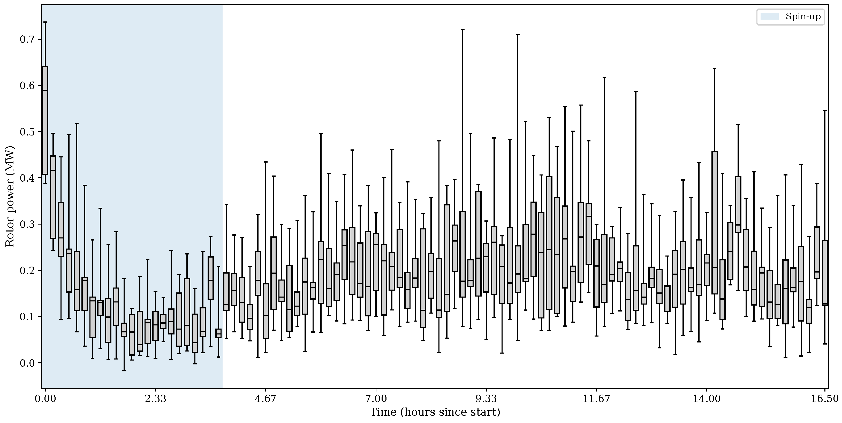
The temporal evolution of turbine power is summarized using boxplots of rotor power across the nine turbines at each output time (Figure 9). This representation highlights both the farm-mean tendency (median line of each box) and the inter-turbine variability (box height and whiskers), which together reflect the combined effects of wake interactions and turbulent inflow fluctuations within the extended-farm setup.
The first 3.5 h of the simulation are treated as a spin-up period (shaded in Figure 9), during which the rotor power exhibits comparatively high median values and a large spread, followed by a rapid reduction as the turbine–wake field develops and adjusts within the periodic domain. After this initial adjustment, the simulation enters a quasi-stationary regime for the remainder of the analysis window, in which the median power fluctuates around an approximately constant level, while the spread across turbines remains pronounced. All reported power statistics in this section are therefore computed over the quasi-stationary period ( 3.5 h to the end of the simulation).
During the quasi-stationary period, the interquartile ranges and whiskers indicate persistent differences in the instantaneous power among turbines, implying systematically different inflow conditions due to spatially varying wake exposure and recovery. The mean turbine power is 192.8 kW lower than the least-waked (upwind) turbine, and the turbine-to-turbine variability is characterized by a mean coefficient of variation of 61.20%, linking the persistent spread in Figure 9 to heterogeneous wake impact across the array. Occasional large whiskers/outliers point to intermittent events with particularly strong deviations from the median (either enhanced inflow or deeper wake deficits), consistent with unsteady wake meandering and turbulence-driven fluctuations that are characteristic of LES wind-farm flows.
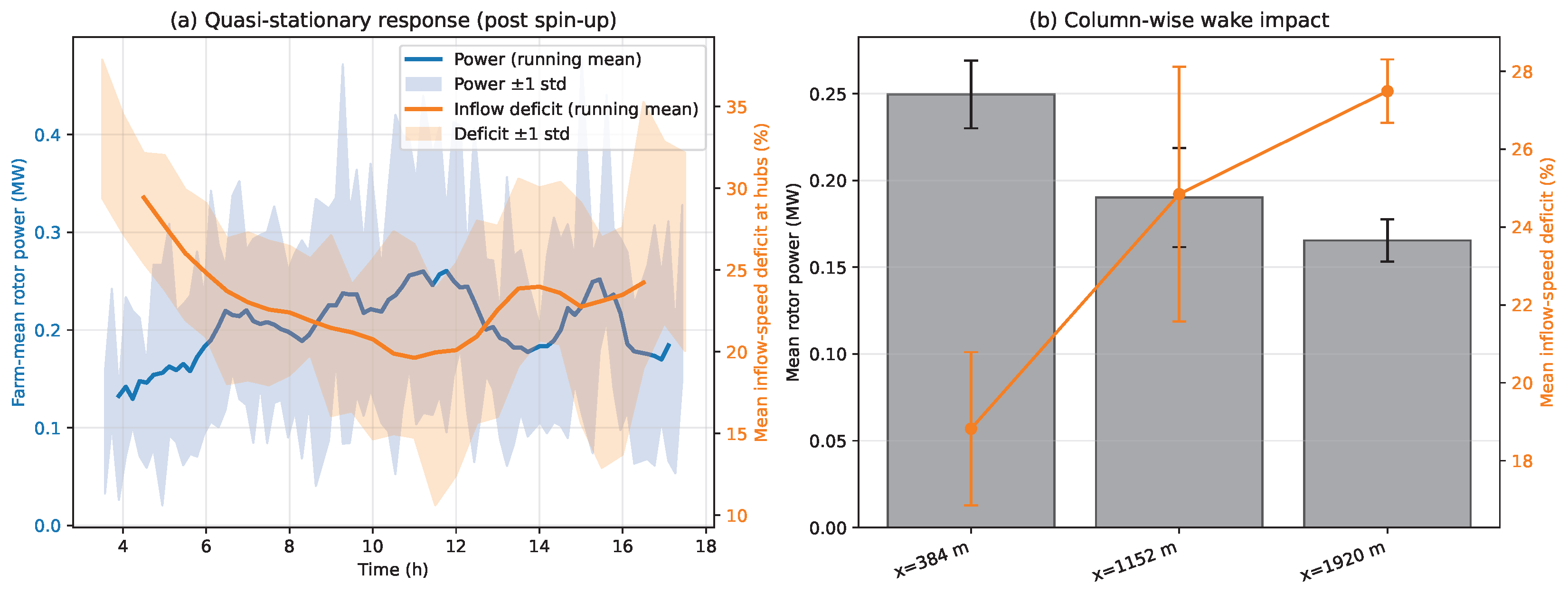
To assess whether the array experiences a stable wake impact under cyclic lateral boundary conditions, we further analyze the temporal evolution of the farm-mean response and the array-scale contrasts (Figure 10). After the initial adjustment period, both the running-mean farm-mean rotor power and the running-mean hub-height inflow-speed deficit at the turbine hubs fluctuate around quasi-stationary levels (Figure 10a), while the shaded bands indicate persistent but bounded inter-turbine variability. The column-wise statistics (Figure 10b) show a systematic array-scale signature, i.e., mean rotor power decreases from the upwind column to downstream columns, concurrent with increasing inflow-speed deficit. This confirms sustained wake interaction across the entire array and provides quantitative evidence that the periodic configuration produces stable interior-farm-like wake coupling over the analyzed period.
Figure 10 also serves as a convergence check for the analysis window. After the initial adjustment period, the running means of both farm-mean rotor power and hub-height inflow-speed deficit approach approximately constant levels, and the inter-turbine spread remains bounded. We therefore define the quasi-stationary regime as the period following this adjustment and compute all reported mean fields, profiles, and power statistics over this common averaging window.
These array-scale diagnostics provide direct support for the intended extended-farm interpretation in the periodic sense: after the initial adjustment, the farm-mean response fluctuates around quasi-stationary levels and the column-wise power/deficit contrasts persist, indicating sustained interior-farm-like wake coupling under cyclic lateral boundary conditions. We therefore refer to this setup as an interior-farm/extended-farm representation under periodic coupling, and we do not interpret it as a validated “deep-farm regime” in the strict benchmark sense.
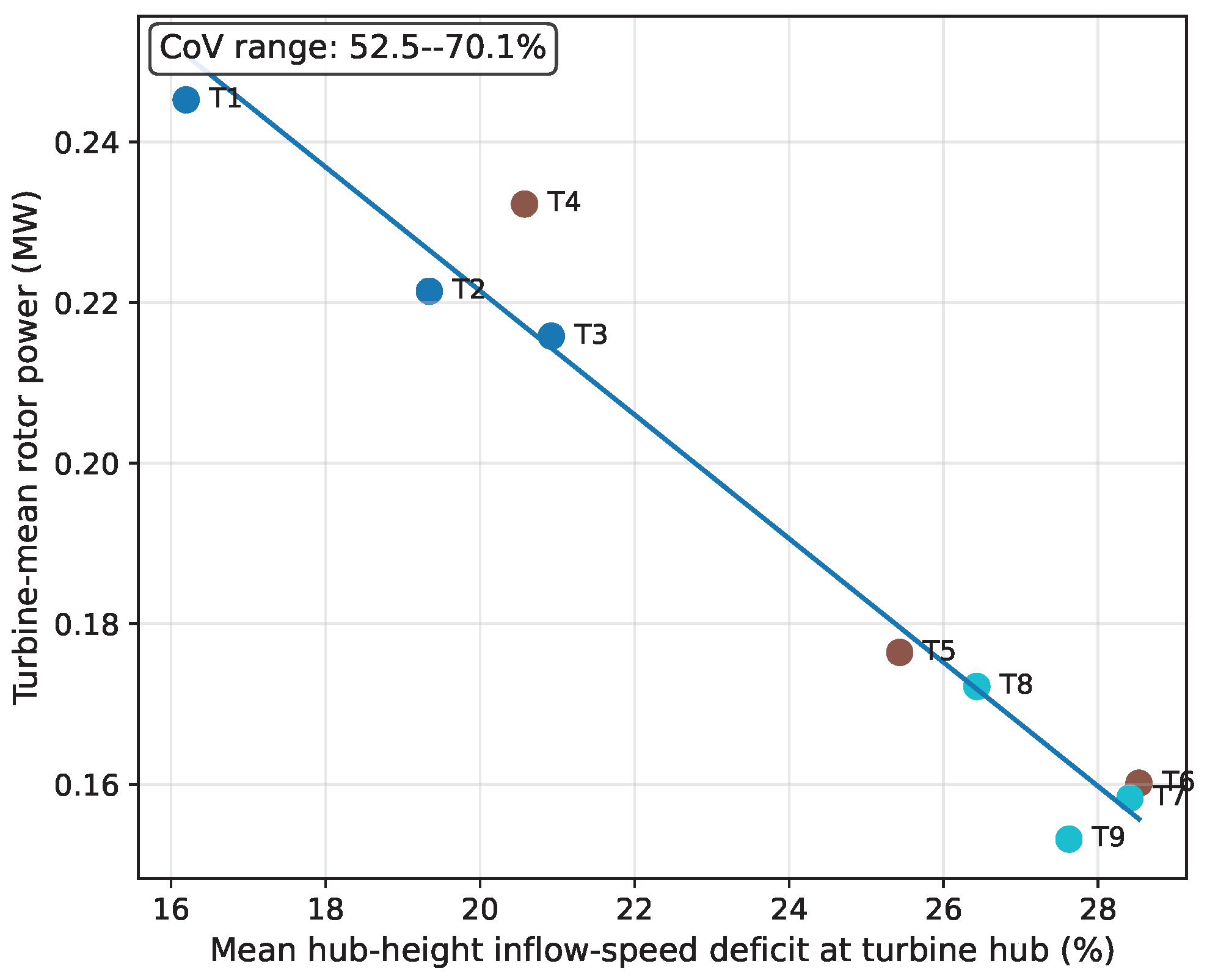
To directly relate the sustained turbine-to-turbine power differences to the flow field, Figure 11 compares the turbine-mean rotor power to the turbine-mean hub-height inflow-speed deficit sampled at each turbine location (relative to the undisturbed background speed U 0 ). The negative relationship confirms that turbines experiencing larger mean wake-induced inflow reduction produce systematically lower mean power, consistent with the hub-height wake corridors in Figure 2 and Figure 3 and the column-wise trend in Figure 10b. Intermittent fluctuations (whiskers/outliers in Figure 9) can be interpreted as periods of transient wake strengthening or partial wake recovery associated with unsteady wake dynamics and turbulence-driven mixing as indicated by elevated SGS-TKE in wake shear layers (Figure 6) and the associated vertical momentum transport (Figure 8).
In addition to the boxplots, Table 5 reports turbine-level mean power and variability metrics together with the corresponding hub-height inflow deficit. The results show systematic power reductions for turbines experiencing larger wake-induced inflow deficits, consistent with the column-wise trend (Figure 10b) and the turbine-level mean power–deficit correlation (Figure 11).

4. Discussion

4.1. Summary of Main Results and Physical Mechanisms

The results provide a consistent picture of wake formation, interaction, and recovery within an extended wind-farm representation, and how these flow processes translate into turbine power variability. At hub height, the normalized mean streamwise velocity field exhibits coherent wake footprints with pronounced velocity deficits that persist over several rotor diameters. These deficits are accompanied by elevated subgrid-scale turbulent kinetic energy concentrated in the wake shear layers, indicating that wake recovery is controlled by the competition between sustained momentum extraction by the turbines and turbulence-enhanced entrainment and mixing at the wake edges. The simultaneous presence of elongated deficit regions and broadened turbulence footprints suggests that wake interactions are not purely local but contribute to array-scale flow modification, consistent with the notion that wind-farm aerodynamics emerge from coupled turbine–ABL dynamics rather than isolated single-wake behavior.
The lateral and vertical velocity components further support this interpretation. The hub-height patterns in v ¯ / U ref indicate persistent cross-stream flow adjustments within and around the wakes, which can be interpreted as a combined effect of turbine forcing and yaw-related wake asymmetry. Similarly, coherent structures in w ¯ / U ref , although smaller in magnitude than the streamwise component, point to secondary circulations that contribute to vertical exchange. Together, these features imply that wake evolution within the array is intrinsically three-dimensional, and that lateral redistribution and vertical motions can influence where and how strongly wakes impinge on downstream turbines. In practical terms, such three-dimensionality is expected to modulate both the mean inflow conditions and the intermittency of wake exposure across the array.
The vertical profiles provide a domain-integrated perspective on these hub-height patterns. The reduction of u ¯ / U ref in the turbine layer is a direct signature of momentum extraction, while the gradual recovery aloft reflects replenishment through turbulent transport. The enhanced turbulence levels in e ¯ / U ref 2 across and above the rotor layer indicate that turbine-induced shear production and wake-related mixing influence a deeper layer than the swept area alone, consistent with the broadened wake footprints observed in plan view. This is corroborated by the turbulent momentum flux profiles. The predominantly negative w u ¯ / U ref 2 indicates the downward transport of higher-momentum air from aloft toward the rotor region, which is a primary mechanism enabling wake recovery and sustaining the mean flow within the turbine layer. The decomposition into resolved and subgrid-scale components shows that a substantial fraction of the vertical transport is carried by resolved eddies, while SGS contributions become more relevant where turbulence length scales approach the grid scale, particularly in strongly sheared regions near the surface and within the rotor layer. The non-zero w v ¯ / U ref 2 further indicates that cross-stream momentum is also redistributed vertically, consistent with wake steering and secondary circulations. Overall, these profiles emphasize that vertical turbulent transport is the key pathway linking turbine forcing, wake recovery, and the mean inflow conditions experienced throughout the array.

4.2. Turbine Power Response and Correlation with Flow-Field Characteristics

The flow-field findings are directly reflected in the rotor power statistics. The boxplot time series demonstrates both a transient adjustment phase and a subsequent quasi-stationary regime with persistent inter-turbine variability. The initial adjustment is consistent with the development of turbulence and the establishment of a wake field within the domain. After this phase, the sustained spread of power across turbines indicates that the array experiences systematically different inflow conditions due to spatially varying wake exposure and recovery. Intermittent excursions and outliers in the power distributions can be interpreted as signatures of unsteady wake dynamics and turbulence-driven variability (e.g., wake meandering and intermittent entrainment events) that temporarily deepen or alleviate wake deficits. From an operational perspective, this behavior implies that farm-level performance is governed not only by the mean wake deficits but also by the temporal variability of wake interaction, which can affect short-term power fluctuations and, by extension, load variability.

4.3. Methodological Discussion, Limitations, and Research Significance

A central methodological aspect of this study is the representation of an extended wind farm using a limited set of turbines. This approach enables sustained turbine–turbine interaction and statistically robust characterization of wake and power behavior at feasible computational cost. Importantly, the resulting flow exhibits features characteristic of wind-farm aerodynamics, including persistent wake footprints, enhanced turbulence in wake shear layers, and a clear momentum-replenishment pathway through downward turbulent transport. The temporal and array-scale diagnostics (Figure 10) further indicate that, after an initial adjustment period, the farm-mean response fluctuates around quasi-stationary levels and that systematic power deficits across the array are consistent with sustained wake coupling in the periodic configuration. By construction, the cyclic lateral boundary conditions recirculate wakes and turbulence structures, which maintains interior-farm interaction and improves statistical sampling for a given computational cost; however, it also implies that finite-farm edge effects and inflow heterogeneity are not represented.
The use of fully periodic lateral boundaries is therefore best interpreted as an interior-farm idealization: wakes and turbulence structures leaving the domain re-enter from the opposite side, enabling sustained wake coupling and efficient statistical sampling. Consequently, the setup does not capture finite-farm edge effects (entrance/exit regions), heterogeneous or time-varying inflow conditions, or mesoscale variability. Absolute values should thus not be interpreted as site-specific predictions but as process-level results under idealized neutral extended-farm conditions.
In this context, the cyclic configuration is interpreted as an interior-farm/extended-farm representation under periodic coupling, i.e., a setup that sustains wake interaction and supports quasi-stationary interior-like statistics, rather than as a validated benchmark “deep-farm regime”. Because yaw misalignment is prescribed and varies among turbines, cross-stream velocity and wake-deflection features are interpreted primarily as yaw-driven signatures, while the extended-farm interpretation relies on yaw-robust metrics such as streamwise deficit, momentum transport, and power statistics.
At the same time, the interpretation of the results must acknowledge the idealized nature of the configuration. The extended-farm representation is designed to capture interior-farm behavior and does not explicitly represent heterogeneous inflow conditions, mesoscale variability, or complex terrain and surface heterogeneity. In addition, quantitative outcomes may depend on model choices such as grid resolution and SGS closure, the turbine parameterization (including airfoil polars and controller settings), and the averaging window used to define U ref and the reported statistics. These factors should be considered when transferring absolute values to real wind farms, while the identified mechanisms linking wakes, turbulence production, momentum transport, and power variability are expected to be robust.

4.4. Future Work Outlook

Future work should extend the present setup to systematically explore the sensitivity of extended-farm wake and power characteristics to atmospheric stability, turbulence intensity, inflow direction, and turbine spacing, as well as to different turbine control strategies (e.g., yaw-based wake steering). Further, comparisons against established wind-energy LES benchmarks and, where available, field observations would strengthen the quantitative interpretation and help constrain uncertainties associated with turbine parameterization and subgrid-scale turbulence modeling. Such developments would provide a pathway toward using PALM-based extended-farm LES not only as a process study tool but also as a basis for evaluating and improving reduced-order wake models and control concepts under realistic atmospheric conditions.

5. Conclusions

This study presented large-eddy simulations of an extended wind-farm configuration using the PALM model system, with the objective of characterizing wake dynamics and their implications for turbine power output. A nine-turbine staggered array was simulated in a computationally efficient setup designed to emulate sustained interior-farm wake coupling under idealized neutral boundary-layer conditions.
At hub height, the time-averaged flow fields revealed coherent wake corridors with a pronounced reduction in turbine inflow conditions. Averaged across all turbines, the mean hub-height inflow speed is reduced by 23.7% relative to an undisturbed background wind speed. The strongest near-wake deficit reaches 71.4% (maximum deficit within 1– 8 D downstream of a turbine), confirming persistent wake interaction over multiple rotor diameters. Wake recovery is accompanied by substantial turbulence enhancement: the rotor-region turbulence intensity increases by 32.2% relative to background, and the peak hub-height SGS-TKE increases by a factor of 6.74 compared to background, with maxima located in the wake shear layers.
The vertically averaged profiles indicate a clear momentum deficit within the turbine layer and gradual recovery aloft, consistent with momentum replenishment through turbulent transport. The streamwise turbulent momentum flux w u ¯ / U ref 2 remains predominantly negative throughout the rotor layer, showing downward transport of higher-momentum air from above as a key recovery mechanism. The resolved/SGS partitioning shows that most of this transport is carried by resolved eddies, while the SGS contribution becomes relatively more important in strongly sheared regions.
Turbine rotor-power statistics exhibit an initial transient adjustment followed by a quasi-stationary regime with persistent inter-turbine variability. The farm-mean turbine power is 192.8 kW, and the amplitude of turbine-to-turbine power fluctuations is substantial, with a mean coefficient of variation of 61.2%. The correlation between turbine-mean power and turbine-mean hub-height inflow deficit demonstrates that sustained power differences across the array are primarily governed by wake-induced inflow reduction, while intermittent excursions are consistent with unsteady wake dynamics and turbulence-driven mixing.
Overall, the results support the use of PALM-based LES for process-level investigation of wind-farm aerodynamics in extended-farm conditions and provide quantitative evidence linking wake deficits, turbulence enhancement, vertical momentum transport, and turbine power variability in an idealized interior-farm regime. Future work should generalize these findings by exploring different atmospheric stabilities, inflow turbulence levels, turbine spacings, and control strategies, and by benchmarking against established wind-energy LES test cases and field observations to further constrain uncertainties and strengthen quantitative interpretation.


Author Contributions

Conceptualization, M.H.S. and M.F.C.E.; methodology, M.H.S. and M.A.M.; software, M.H.S.; validation, I.K.M., M.A.M. and M.F.C.E.; formal analysis, M.H.S.; investigation, M.F.C.E.; resources, M.H.S.; data curation, I.K.M.; writing—original draft preparation, M.H.S.; writing—review and editing, I.K.M.; visualization, M.A.M.; supervision, I.K.M. All authors have read and agreed to the published version of the manuscript.

Funding

This research received no external funding.

Data Availability Statement

The raw data supporting the conclusions of this article will be made available by the authors on request.

Acknowledgments

The simulations were carried out on the supercomputer Lise at the NHR@ZIB center. NHR@ZIB is one of nine centers within the Alliance for National High Performance Computing (Nationales Hochleistungsrechnen, NHR). It is a facility of the Zuse Institute Berlin (ZIB) and provides scientific computing infrastructure to support science and research throughout Germany. Compute time was granted through the peer-reviewed allocation process organized by the NHR scientific board (Wissenschaftlicher Ausschuss). We gratefully acknowledge the support by the NHR@ZIB team and the supra-regional NHR competence network.

Conflicts of Interest

The authors declare no conflicts of interest.

Abbreviations

The following abbreviations are used in this manuscript:
ABLAtmospheric Boundary Layer
ADM-RActuator Disk Model with Rotation
BEMBlade-Element Momentum (method)
CFDComputational Fluid Dynamics
LESLarge-Eddy Simulation
PALMParallelized Large-Eddy Simulation Model (PALM model system)
RANSReynolds-Averaged Navier–Stokes
SGSSubgrid-Scale
TKETurbulent Kinetic Energy
WTWind Turbine
WTMWind Turbine Model (PALM module)

Appendix A. Basic Convergence Assessment

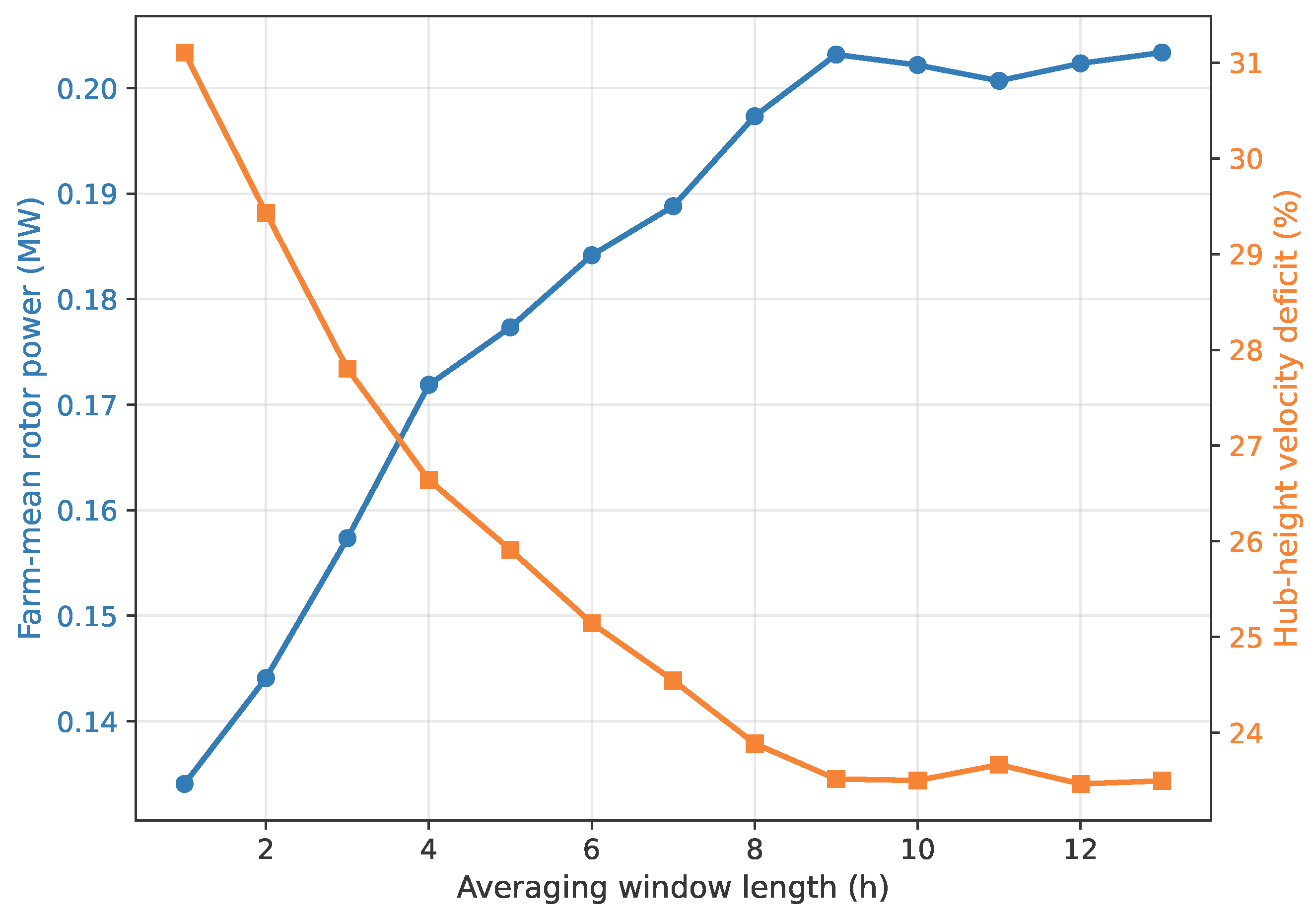
To support the definition of the post-spin-up quasi-stationary regime used throughout this study, we evaluate the convergence of two representative diagnostics as a function of averaging-window length after the spin-up period (3.5 h). Specifically, we compute the cumulative mean farm-mean rotor power and the cumulative mean hub-height inflow-speed deficit sampled at the turbine hubs, using averaging windows of 1 h, 2 h, … up to the end of the available post-spin-up period. Figure A1 shows that both quantities approach approximately stable values as the averaging window increases, supporting the robustness of the mean statistics reported in Section 3.
Figure A1. Basic convergence assessment for representative diagnostics computed over cumulative averaging windows after the spin-up period (3.5 h). Shown are the farm-mean rotor power (left axis) and the mean hub-height inflow-speed deficit at turbine hubs (right axis) as a function of averaging-window length.
Energies 19 02391 g0a1

Appendix B. Quantitative Wake Metrics

This appendix presents the quantitative wake characterization extracted from the time-averaged hub-height ( z = 140   m ) streamwise velocity field discussed in Section 3. All metrics are computed along the local wake centerline, defined parallel to the mean inflow direction, and normalized by the rotor diameter D = 126   m and the hub-height reference velocity U ref .
Figure A2. Time-averaged centerline velocity deficit Δ u ¯ / U ref = 1 u ¯ / U ref as a function of downstream distance x / D for turbines T1–T9. Solid lines are sampled directly from the LES field; dashed lines are least-squares power-law fits of the form Δ u ¯ / U ref = A ( x / D ) k , with the fitted exponent k given in Table A1. The non-monotonic behavior near x / D 1.5 reflects the transition from the near-wake recirculation zone to the expanding far-wake region.
Energies 19 02391 g0a2
Figure A3. Gaussian wake half-width σ / D as a function of downstream distance x / D for turbines T1–T9. At each cross-section, a Gaussian function is fitted to the lateral velocity-deficit profile; σ is the resulting standard deviation. Turbines T3, T8, and T9 exhibit anomalously large or non-monotonic widths at large x / D values, which indicates that the sampled lateral profiles intercept the wakes of adjacent turbines and can no longer be described by a single-peak Gaussian at those downstream distances.
Energies 19 02391 g0a3
Figure A4. Lateral velocity-deficit profiles for turbine T1 at downstream distances x / D = 2 , 4 , 6 , 8 (left to right). The deficit is sampled perpendicular to the inflow direction across ± 3 D of lateral extent. Dashed lines show Gaussian fits whose parameters ( Δ u ¯ 0 , σ , y 0 ) are used to populate Table A1 and Figure A3. The progressive narrowing of the deficit peak and the slight lateral displacement of the profile centroid are consistent with the helical wake meandering visible in the instantaneous velocity fields.
Energies 19 02391 g0a4
Table A1. Summary of quantitative wake metrics for turbines T1–T9. U in / U ref : rotor-disk-averaged inflow velocity normalized by U ref ; Δ u ¯ max : maximum centerline deficit observed within the sampled range; Δ u ¯ | 3 D , Δ u ¯ | 6 D , Δ u ¯ | 9 D : centerline deficit at specific downstream distances; x 95 % / D : downstream distance at which the deficit drops below 0.05 (95% recovery of U ref ), with >12 indicating that the threshold is not reached within the sampled domain; k: power-law decay exponent fitted to the far-wake centerline deficit.
Turbine U in / U ref Δ u ¯ max Δ u ¯ | 3 D Δ u ¯ | 6 D Δ u ¯ | 9 D x 95 % / D k
T10.7190.5280.3770.2480.161>120.794
T20.6950.5680.3920.2510.162>120.820
T30.6790.5710.3920.2230.08511.01.064
T40.6830.5650.3830.2480.155>120.867
T50.6400.5960.3980.2660.175>120.801
T60.6080.6170.3970.2670.182>120.710
T70.6130.6150.3850.0980.0187.51.318
T80.6290.5860.3840.1210.053>121.191
T90.6180.6050.3920.2020.202>120.684
The metrics in Table A1 reveal a clear progression in wake from the front-row to the interior turbines. The rotor-disk inflow ratio U in / U ref decreases monotonically from 0.719 for T1 (first row, unobstructed inflow) to 0.608 for T6 (interior, third row), a reduction of approximately 15%. Maximum centerline deficits increase correspondingly, reaching up to 0.617 for T6, while the power-law decay exponent k spans the range 0.68 1.32 , indicating substantial variability in far-wake recovery rates across turbine positions. Turbines T7 and T8 stand out with notably faster centerline recovery (higher k, lower deficits at 6 D 9 D ), which is consistent with the enhanced turbulent mixing visible in the hub-height velocity maps for those positions. None of the turbines, with the exception of T7 ( x 95 % / D = 7.5 ) and T3 ( x 95 % / D = 11.0 ), achieves 95% recovery of U ref within the 12 D sampled range, underlining the persistence of wake deficits across the entire wind farm layout.

References

  1. Qiao, Y.; Liu, Y.; Chen, Y.; Han, S.; Wang, L. Power Generation Performance Indicators of Wind Farms Including the Influence of Wind Energy Resource Differences. Energies 2022, 15, 1797. [Google Scholar] [CrossRef] [Scilit]
  2. Liu, Y.; Zhao, Z.; Liu, Y.; Liu, H.; Wei, S.; Ma, Y.; Ling, Z.; Luo, Q. Combined wake control of aligned wind turbines for power optimization based on a 3D wake model considering secondary wake steering. Energy 2024, 308, 132900. [Google Scholar] [CrossRef] [Scilit]
  3. Wu, Y.T.; Porté-Agel, F. Large-Eddy Simulation of Wind-Turbine Wakes: Evaluation of Turbine Parametrisations. Bound. Layer Meteorol. 2010, 138, 345–366. [Google Scholar] [CrossRef] [Scilit]
  4. Sedaghatizadeh, N.; Arjomandi, M.; Kelso, R.; Cazzolato, B.; Ghayesh, M.H. Modelling of wind turbine wake using large eddy simulation. Renew. Energy 2018, 115, 1166–1176. [Google Scholar] [CrossRef] [Scilit]
  5. Boettcher, M.; Hoffmann, P.; Lenhart, H.J.; Schlünzen, K.H.; Schoetter, R. Influence of large offshore wind farms on North German climate. Meteorol. Z. 2015, 24, 465–480. [Google Scholar] [CrossRef] [Scilit]
  6. Salim, M.H.; Schlünzen, K.H.; Grawe, D.; Boettcher, M.; Gierisch, A.M.U.; Fock, B.H. The microscale obstacle-resolving meteorological model MITRAS v2.0: Model theory. Geosci. Model Dev. 2018, 11, 3427–3445. [Google Scholar] [CrossRef] [Scilit]
  7. Vollmer, L.; Steinfeld, G.; Kühn, M. Transient LES of an offshore wind turbine. Wind Energy Sci. 2017, 2, 603–614. [Google Scholar] [CrossRef] [Scilit]
  8. Krutova, M.; Paskyabi, M.B.; Nielsen, F.G.; Reuder, J. Evaluation of Gaussian wake models under different atmospheric stability conditions: Comparison with large eddy simulation results. J. Phys. Conf. Ser. 2020, 1669, 012016. [Google Scholar] [CrossRef] [Scilit]
  9. Witha, B.; Steinfeld, G.; Heinemann, D. High-Resolution Offshore Wake Simulations with the LES Model PALM. In Wind Energy-Impact of Turbulence; Springer: Berlin/Heidelberg, Germany, 2014; pp. 175–181. [Google Scholar] [CrossRef] [Scilit]
  10. Witha, B.; Steinfeld, G.; Dörenkämper, M.; Heinemann, D. Large-eddy simulation of multiple wakes in offshore wind farms. J. Phys. Conf. Ser. 2014, 555, 012108. [Google Scholar] [CrossRef] [Scilit]
  11. Vollmer, L.; Steinfeld, G.; Heinemann, D.; Kühn, M. Estimating the wake deflection downstream of a wind turbine in different atmospheric stabilities: An LES study. Wind Energy Sci. 2016, 1, 129–141. [Google Scholar] [CrossRef] [Scilit]
  12. Krutova, M.; Bakhoday-Paskyabi, M.; Reuder, J.; Nielsen, F.G. Self-nested large-eddy simulations in PALM model system v21.10 for offshore wind prediction under different atmospheric stability conditions. Geosci. Model Dev. 2023, 16, 3553–3564. [Google Scholar] [CrossRef] [Scilit]
  13. Cao, L.; Ge, M.; Gao, X.; Du, B.; Li, B.; Huang, Z.; Liu, Y. Wind farm layout optimization to minimize the wake induced turbulence effect on wind turbines. Appl. Energy 2022, 323, 119599. [Google Scholar] [CrossRef] [Scilit]
  14. Yang, R.; Cui, T.; Chen, Z.; Ma, S.; Ping, H.; Wei, F.; Gao, Z.; Lu, G.; Liu, H.; Zhang, L. Review on Dynamic Inflow Sensing Layout Optimization for Large-Scale Wind Farms: Wake Modeling, Data-Driven Prediction, and Multi-Objective Uncertainty Optimization. Energies 2026, 19, 810. [Google Scholar] [CrossRef] [Scilit]
  15. Sanderse, B.; van der Pijl, S.; Koren, B. Review of computational fluid dynamics for wind turbine wake aerodynamics. Wind Energy 2011, 14, 799–819. [Google Scholar] [CrossRef] [Scilit]
  16. Shives, M.; Crawford, C. Adapted two-equation turbulence closures for actuator disk RANS simulations of wind & tidal turbine wakes. Renew. Energy 2016, 92, 273–292. [Google Scholar] [CrossRef] [Scilit]
  17. Naderi, S.; Parvanehmasiha, S.; Torabi, F. Modeling of horizontal axis wind turbine wakes in Horns Rev offshore wind farm using an improved actuator disc model coupled with computational fluid dynamic. Energy Convers. Manag. 2018, 171, 953–968. [Google Scholar] [CrossRef] [Scilit]
  18. Rezaeiha, A.; Montazeri, H.; Blocken, B. CFD analysis of dynamic stall on vertical axis wind turbines using Scale-Adaptive Simulation (SAS): Comparison against URANS and hybrid RANS/LES. Energy Convers. Manag. 2019, 196, 1282–1298. [Google Scholar] [CrossRef] [Scilit]
  19. Qian, Y.; Wang, T.; Yuan, Y.; Zhang, Y. Comparative study on wind turbine wakes using a modified partially-averaged Navier-Stokes method and large eddy simulation. Energy 2020, 206, 118147. [Google Scholar] [CrossRef] [Scilit]
  20. Ghaisas, N.S.; Archer, C.L.; Xie, S.; Wu, S.; Maguire, E. Evaluation of layout and atmospheric stability effects in wind farms using large-eddy simulation. Wind Energy 2017, 20, 1227–1240. [Google Scholar] [CrossRef] [Scilit]
  21. Chanprasert, W.; Sharma, R.; Cater, J.; Norris, S. Large Eddy Simulation of wind turbine wake interaction in directionally sheared inflows. Renew. Energy 2022, 201, 1096–1110. [Google Scholar] [CrossRef] [Scilit]
  22. Cheung, L.; Yalla, G.; Brown, K.; deVelder, N.; Hsieh, A.; Herges, T.; Houck, D.; Maniaci, D.; Sakievich, P.; Abraham, A. Modification of wind turbine wakes by large-scale, convective atmospheric boundary layer structures. J. Renew. Sustain. Energy 2024, 16, 063304. [Google Scholar] [CrossRef] [Scilit]
  23. Breton, S.P.; Sumner, J.; Sørensen, J.N.; Hansen, K.S.; Sarmast, S.; Ivanell, S. A survey of modelling methods for high-fidelity wind farm simulations using large eddy simulation. Philos. Trans. R. Soc. Math. Phys. Eng. Sci. 2017, 375, 20160097. [Google Scholar] [CrossRef] [Scilit]
  24. Mehta, D.; van Zuijlen, A.; Koren, B.; Holierhoek, J.; Bijl, H. Large Eddy Simulation of wind farm aerodynamics: A review. J. Wind Eng. Ind. Aerodyn. 2014, 133, 1–17. [Google Scholar] [CrossRef] [Scilit]
  25. Porté-Agel, F.; Wu, Y.T.; Lu, H.; Conzemius, R.J. Large-eddy simulation of atmospheric boundary layer flow through wind turbines and wind farms. J. Wind Eng. Ind. Aerodyn. 2011, 99, 154–168. [Google Scholar] [CrossRef] [Scilit]
  26. Lu, H.; Porté-Agel, F. Large-eddy simulation of a very large wind farm in a stable atmospheric boundary layer. Phys. Fluids 2011, 23, 065101. [Google Scholar] [CrossRef] [Scilit]
  27. Maronga, B.; Banzhaf, S.; Burmeister, C.; Esch, T.; Forkel, R.; Fröhlich, D.; Fuka, V.; Gehrke, K.F.; Geletič, J.; Giersch, S.; et al. Overview of the PALM model system 6.0. Geosci. Model Dev. 2020, 13, 1335–1372. [Google Scholar] [CrossRef] [Scilit]
  28. Anders, J.; Schubert, S.; Sauter, T.; Tunn, S.; Schneider, C.; Salim, M. Modelling the impact of an urban development project on microclimate and outdoor thermal comfort in a mid-latitude city. Energy Build. 2023, 296, 113324. [Google Scholar] [CrossRef] [Scilit]
  29. Dörenkämper, M.; Witha, B.; Steinfeld, G.; Heinemann, D.; Kühn, M. The impact of stable atmospheric boundary layers on wind-turbine wakes within offshore wind farms. J. Wind Eng. Ind. Aerodyn. 2015, 144, 146–153. [Google Scholar] [CrossRef] [Scilit]
  30. Chatterjee, T.; Peet, Y.T. Contribution of large scale coherence to wind turbine power: A large eddy simulation study in periodic wind farms. Phys. Rev. Fluids 2018, 3, 034601. [Google Scholar] [CrossRef] [Scilit]
  31. Stipa, S.; Ajay, A.; Allaerts, D.; Brinkerhoff, J. TOSCA–An open-source, finite-volume, large-eddy simulation (LES) environment for wind farm flows. Wind Energy Sci. 2024, 9, 297–320. [Google Scholar] [CrossRef] [Scilit]
  32. Roache, P.J. Perspective: A Method for Uniform Reporting of Grid Refinement Studies. J. Fluids Eng. 1994, 116, 405–413. [Google Scholar] [CrossRef] [Scilit]
  33. Hefny, M.M.; Ooka, R. CFD analysis of pollutant dispersion around buildings: Effect of cell geometry. Build. Environ. 2009, 44, 1699–1706. [Google Scholar] [CrossRef] [Scilit]
  34. Mohamed, M.A.; Maksoud, T.; Santos, R.J.; Salim, M.H.; Esmail, M.F. Numerical simulation of the aerodynamic performance of a novel micro-aerial vehicle mimicking a locust. Ain Shams Eng. J. 2021, 12, 2935–2945. [Google Scholar] [CrossRef] [Scilit]
  35. Abo-Zahhad, E.M.; Hachicha, A.A.; Mistarihi, M.Z.; Salim, M.H.; Esmail, M.F. Optimization of ground material properties for enhanced solar chimney power plant efficiency: A CFD and RSM approach. Energy Rep. 2025, 13, 3929–3945. [Google Scholar] [CrossRef] [Scilit]
Figure 1. Plan-view schematic of the domain showing turbine hub locations, with annotations of spacings in meters and in units of D.
Energies 19 02391 g001
Figure 2. Time-averaged streamwise velocity at hub height ( z = 140 m), normalized by the hub-height reference speed U ref . The turbine locations (T1–T9) are indicated. Axes are shown in rotor-diameter units ( x / D , y / D ).
Energies 19 02391 g002
Figure 3. Time-averaged hub-height wind-speed magnitude | V ¯ h | at z = 140 m, normalized by U ref . The turbine locations (T1–T9) are indicated. Axes are shown in rotor-diameter units ( x / D , y / D ).
Energies 19 02391 g003
Figure 4. Time-averaged lateral velocity component at hub height ( z = 140 m), normalized by U ref . The turbine locations (T1–T9) are indicated. Axes are shown in rotor-diameter units ( x / D , y / D ).
Energies 19 02391 g004
Figure 5. Time-averaged vertical velocity component at hub height ( z = 140 m), normalized by U ref . The turbine locations (T1–T9) are indicated. Axes are shown in rotor-diameter units ( x / D , y / D ).
Energies 19 02391 g005
Figure 6. Time-averaged subgrid-scale turbulent kinetic energy e ¯ at hub height ( z = 140 m), normalized by U ref 2 . The turbine locations (T1–T9) are indicated. Axes are shown in rotor-diameter units ( x / D , y / D ).
Energies 19 02391 g006
Figure 7. Vertically averaged profile of the normalized mean streamwise velocity ( u ¯ / U ref ), mean lateral velocity ( v ¯ / U ref ), and normalized subgrid-scale turbulent kinetic energy, e ¯ / U ref 2 , as a function of height z.
Energies 19 02391 g007
Figure 8. Vertically averaged profile of the normalized vertical flux of lateral momentum, w u ¯ / U ref 2 and w v ¯ / U ref 2 , decomposed into resolved and subgrid-scale (SGS) contributions.
Energies 19 02391 g008
Figure 9. Temporal evolution of turbine rotor power shown as boxplots across the nine turbines at each time step. The shaded region denotes the spin-up period (0 h– 3.5 h); statistics reported in Section 3.4 are computed over the subsequent quasi-stationary period. The central line denotes the median, boxes indicate the interquartile range, and whiskers represent the spread of turbine power outputs. Time is given in hours since simulation start; rotor power is reported in MW.
Energies 19 02391 g009
Figure 10. Array-scale stability and wake impact under cyclic lateral boundary conditions. (a) Running-mean farm-mean rotor power and running-mean hub-height inflow-speed deficit at the turbine hubs; shading indicates ± 1 standard deviation across turbines at each time. (b) Column-wise means (grouped by turbine x-location) of rotor power (bars) and inflow-speed deficit (markers) with ± 1 standard deviation across turbines.
Energies 19 02391 g010
Figure 11. Relationship between turbine-mean rotor power and turbine-mean hub-height inflow-speed deficit (relative to the undisturbed background speed U 0 ), computed from hub-height flow fields sampled at turbine locations. Points are labeled by turbine ID (T1–T9).
Energies 19 02391 g011
Table 1. Turbine hub coordinates and prescribed initial yaw angles. Coordinates are in meters.
Turbine ID x h y h z h γ 0 (deg)
T1384640140 20
T2384128014010
T338419201400
T4115232014030
T51152960140 20
T61152160014010
T719206401400
T81920128014030
T919201920140 20
Table 2. Wind-turbine geometric and control parameters used for all turbines in the array.
ParameterValue
Number of turbines, n t 9
Hub height, z h 140 m
Rotor radius, R63 m
Rotor diameter, D = 2 R 126 m
Nacelle radius1.5 m
Tower diameter4.0 m
Rated generator power, P rated 5.29661 × 10 6  W
Rotor speed (initial/prescribed in module)0.9
Tilt angle 0
Speed controlenabled
Pitch control (initial pitch angle 0 )enabled
Yaw controlenabled
Yaw speed0.01
Tower drag coefficient, C d 1.2
Segment length (tangential)1.0 m
Segment width (radial)0.5 m
Number of airfoils8
Table 3. Numerical setup and boundary conditions used in the PALM simulations.
ItemValue
Domain and grid
Grid points n x = 575 , n y = 559 , n z = 256
Horizontal grid spacing Δ x = Δ y = 4  m
Vertical grid spacing Δ z = 2  m (up to z = 350  m)
Vertical stretchingfactor 1.04 above z = 350  m, Δ z max = 60  m
Domain size (physical) L x = 2304  m, L y = 2240  m, L z 1545  m
Numerics and turbulence modeling
Time integrationthird-order Runge–Kutta (RK3)
Advection (momentum, scalars)Wicker–Skamarock, 5th order
SGS turbulence closure1.5-order SGS-TKE closure (LES mode)
Governing-equation approximationBoussinesq approximation
Pressure solvermultigrid (W-cycle); Gauss–Seidel iterations
Stratificationneutral; no prognostic p t equation; p t = 300  K
Boundary/initial conditions and forcing
Lateral boundariescyclic (left/right) and cyclic (north/south)
Top boundary forcinggeostrophic forcing at the model top
Turbulence triggeringrandom perturbations: amplitude 0.25 m s−1
Table 4. Grid-convergence assessment using two refinement steps. For each target variable, ε rms denotes the RMS relative difference between the two grids of the step. The GCI values are computed conservatively using safety factor F = 5 and order p = 2 .
Refinement Step r = l fine / l coarse uvwRotor Power
ε rms (%)GCI (%) ε rms (%)GCI (%) ε rms (%)GCI (%) ε rms (%)GCI (%)
Coarse-2 → Coarse-10.7500.603.860.704.501.006.430.503.21
Coarse-1 → Fine0.6670.401.600.602.400.803.200.451.80
Table 5. Turbine-level power statistics and hub-height inflow conditions computed over the post-spin-up (quasi-stationary) period. The inflow deficit is defined relative to the undisturbed background speed U 0 .
Turbine P ¯ (MW) σ P (MW)CoV (%)Deficit (%)Column (x)
T10.2750.12946.816.2
T20.2460.14057.119.3384
T30.2280.11148.720.9
T40.2290.10847.120.6
T50.1810.09451.925.41152
T60.1610.09458.328.5
T70.1600.09257.228.4
T80.1820.09552.026.41920
T90.1540.07749.927.6
Disclaimer/Publisher’s Note: The statements, opinions and data contained in all publications are solely those of the individual author(s) and contributor(s) and not of MDPI and/or the editor(s). MDPI and/or the editor(s) disclaim responsibility for any injury to people or property resulting from any ideas, methods, instructions or products referred to in the content.