A Two-Stage Energy and Service Market Framework Involving Unit Commitment and Network-Based Redispatch

Abstract

The provision of power and grid services requires the co-ordination between Day-Ahead Market (DAM) and Ancillary Service Market (ASM) to attain reserve services and technically feasible operating conditions for market players and for the network. In this context, this work proposes a multi-stage approach to evaluate the dispatched power to balance the forecast updates of renewable energy sources and load from DAM to ASM, taking into account network and Unit Commitment (UC) constraints. The DAM is solved considering a zonal market framework and neglecting the UC constraints. Then, a mechanism to adjust the ASM bids is developed, defining time-varying costs for each regulation. Finally, the ASM is modelled as a network-constrained UC and economic redispatch (NCUCER) optimization problem, aiming at minimizing the overall cost, in order to procure secondary reserve requirement and to adjust the DAM schedules, taking into account network and UC constraints and balancing forecast updates. DC load flow sensitivity factors are exploited to evaluate the influence of redispatch actions and forecast updates on the observed power flow. This procedure is applied to NREL 118-Bus Test System assessing its performances throughout a yearly time horizon.

1. Introduction

Network security issues related to renewable energy sources (RES) and load forecast errors are faced by transmission system operators (TSOs) by means of redispatching and balancing services. Balancing resources are exploited to restore system frequency in real-time (RT) operation, whereas redispatch mechanism can be used when energy market outcomes do not fulfil power flow bounds [1], showcasing a high potential for cost optimization to remedy network congestions and to compensate for power fluctuations. Redispatch mechanism is managed by different procurement and remuneration models, depending on national grid rules [2].

In the last years, coupled energy markets were created in order to increase the utilisation of generation sources among European market operator members (Nominated Electricity Market Operators, NEMOs), resulting in Single Day-ahead Coupling and Single Intraday Coupling markets [3,4]. This new joint governance structure aims at achieving a better co-operation between NEMOs and TSOs. In fact, the inputs of these markets are the network capacities and constraints provided by the TSOs and the bids and offers provided by the NEMOs. In this structure, the ancillary service provision/delivery is managed in a successive market platform, where a harmonized market among European regions is still in a preliminary stage with some pilot projects, due to the different market frameworks [5]. Further insights into European market context and pilot projects are provided in [6].

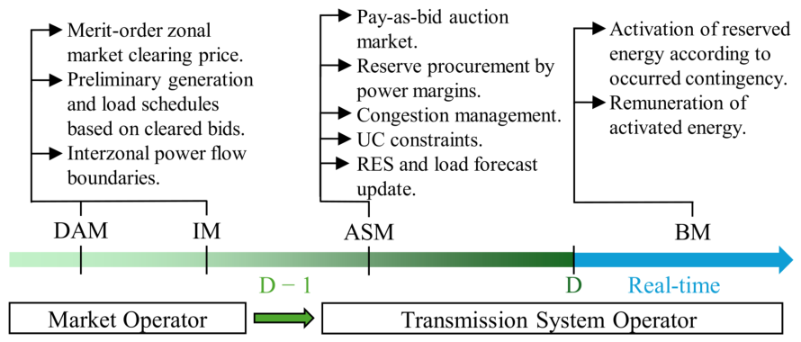
Among European countries, Italian TSO has developed a comprehensive expertise in handling generating units and network constraints in market sessions downstream merit-order energy markets, as highlighted in Figure 1 [7]. In particular, the energy markets are the Day-ahead (DAM) and the Intraday (IM) markets, managed by Italian Market Operator, aiming at maximising the social welfare through a merit-order zonal clearing price mechanism. In this session, the main energy amount is traded defining the preliminary generation and load schedules considering step-wise bids and interzonal power flow constraints. Downstream, the Ancillary Service market (ASM) sessions take place, managed by the TSO, to provide the required services according to a pay-as-bid auction market. Specifically, the TSO, based on energy market schedules, can redispatch units to procure upward and downward power margin, depending on the needed reserve, while complying with line power flows and unit commitment (UC) constraints along with the RES and load forecasts updates. Finally, Balancing Market (BM) is carried out over the whole day, activating the amounts reserved in ASM to mitigate any contingency, e.g., load and RES mismatches, generation outage, etc., and remunerating only the activated energy.

On the methodological point of view, security-constrained unit commitment (SCUC) and economic dispatch (ED) have been extensively investigated [8,9]. These works provide comprehensive state-of-the-art reviews of the mathematical modeling and solving of these problems, tracing their evolution from deterministic approaches to stochastic and robust optimization frameworks, while emphasizing the integration of intermittent RES in the current energy context of decarbonization.

While these works establish a robust foundation for preventive generation scheduling—addressing the uncertainty management [10,11], grid security and more recently computational efficiency in terms of flexible temporal resolution [12]—only a few works deal with market-based power redispatch to update the production levels of generating units depending on power system operating conditions. The amount of redispatched power derives from an optimization problem aiming at solving congestions [10,11,12,13,14], balancing RES and/or load due to uncertainties [10,11,15,16], facing outage in the presence of extreme weather events [17], or procuring reserve requirements [18,19]. In the most employed deterministic formulations, units are allowed to be started-up or shut-down to provide redispatch, adopting integer variables, resulting in a mixed-integer linear programming (MILP) problem [14,20], and other formulations are seldom used, such as linear programming [10,11,16], dynamic non-linear programming [21], mixed-integer non-linear programming [13], or robust optimization [18]. The optimization problem has an economic purpose, mainly aiming at minimizing active power redispatch and start-up costs, and further costs can be due to shut-down, reserve provision or deployment, RES and/or load curtailment [10,15,16,17,18]. On the other hand, technical objective functions involve congestions mitigation [10,13] or the minimization of the overload probability risk [11]. In this regard, the inclusion of both technical and economic constraints is therefore necessary, albeit computationally costly, in order to ensure that the market outcomes are technically feasible. In addition to power balance and power flow limits, modeled by means of sensitivity factors [10,11,13] or DC load flow (DCLF) equations [15,17,18], constraints could involve generator technical limits [14,15,16,17,21], RES and/or load curtailment limits [16,17], along with reserve provision, deployment or allocation limits [15,18].

Most traditional UC/ED mathematical models focus on either the DAM or the ASM, overlooking the fact that decisions made in the former heavily constrain the latter. In particular, in the redispatching action modeling the status of generators (on/off) is often considered as fixed by the DAM, so that only units that are already in operation are able to adjust their power production in the real-time markets [22]. However, the inherent RES stochasticity makes these methods excessively rigid and unrealistic requiring a re-evaluation of the operational status during ASM phase.

A well-established line of research addresses the interdependence between markets using multi-stage models. The co-ordination between consecutive market sessions has been investigated, especially for energy and real-time markets in the American framework, as in [23], dealing with a two-stage day-ahead (DA) clearing model for the energy and RT markets in the presence of high RES penetration considering fast-start generator behaviors as non-spinning reserve providers. In particular, the energy market optimization problem embeds the required amount of energy and reserves. Moreover, the work proposed in [24] deals with a stochastic model predictive control scheme used to handle the uncertainty related to generation and load profiles combining Chance-Constrained and Machine Learning techniques. This approach can be applied to participate simultaneously in different energy markets. The authors of [25] analyze the impact of wind farm (WF) power forecast on the co-ordination between energy and RT markets, and particularly focusing on cost implication between DA and RT due to WF uncertainties, handled by the system operator through anticipated RT adjustment bids, aiming to minimize the costs associated with conventional thermal generators and WF generators. In [26], a day-ahead reserve determination method based on two-stage stochastic programming approach is proposed. In the first stage the commitment of thermal units is carried out, whereas in the second stage the operation of the system with and without the failure of key thermal units is evaluated. Further methods, aims, and perspectives on market sessions co-ordination are available in the review paper [27].

Regarding the European framework, the work developed in [19] defines three optimization problems to model consecutive markets connecting intraday and reserve markets, in order to find feasible power profiles, provide secondary reserve (SR), and deploy the energy and SR, respectively, defining unit-state constraints for the already committed units. In addition, ref. [28] presents a meta-analysis of the evolution of ASMs and the underlying regulatory trade-offs, aiming to provide an evaluation of each trend regarding the architecture, the services, and the products of the ASMs, based on the level of agreement of the two main counter-parties: the TSO who manages the system and the Balancing Services Provider (BSP) that delivers the service. Moreover, in [29] it is noted that European zonal markets neglect congestion within a zone during the DAM phase, necessitating a subsequent generation redispatch. In the Italian context, instead, ref. [30] explores how UC and ED algorithms are integrated in the current market structure and exploited by the TSO to ensure grid security, pointing out that investigating market-based redispatch mechanisms becomes even more crucial for correcting imbalances and addressing physical network constraints without altering economic price signals. The work proposed in [6] presents three models to represent DAM, ASM, and the RT market in a renewable-dominated power system. In particular, the market configurations are compared to commit the reserves in DAM, ASM, or in a joined co-optimized market. The problem considers units and network constraints along with reserve provision considering RES and load uncertainties.

From the analysis illustrated so far, the need for a clearing procedure accounting for the DAM-ASM interaction arises in order to draw energy price signals in DAM for all participants, including final users, and solving the technical feasibility for units and network in the specific ASM framework for selected operators. To this purpose, in this paper, a multi-stage procedure for modeling the electricity market sessions up to ASM schedules is presented. This method, accounting for network operator viewpoint, is fourfold and includes: the merit-order zonal DAM clearance, that provides an initial generation profile coping with forecast load demand and RES generation based on marginal cost bids; the adjustment of ASM bids depending on DAM outcomes and technical operational limits of the dispatchable generators; the preliminary evaluation of DAM solution feasibility and network sensitivities; the nodal ASM solution by redispatching generator schedules through a MILP optimization problem. The proposed ASM model aims at minimizing redispatching costs, fulfilling power flow and UC constraints, procuring SR and balancing RES and load forecast updates. To this purpose, a Network-Constrained UC and economic redispatch (NCUCER) optimization problem is proposed, accounting for specific influence of unit status after DAM on operation modes in ASM. Particularly, the redispatching actions are referred to the start-up (SU) and shut-down (SD) constraints of dispatchable thermal (DT) units which could arise downstream of the energy market, along with different technical constraints for DT and dispatchable hydroelectric (DH) units. The approach is applied to the modified version of the IEEE 118-bus test system [31], analyzing proper sensitivities and comparing with a benchmark DAM market model including UC and reserve constraints [32,33].

The main contributions of this work can be summarized:

• Modeling the sequential interaction between zonal DAM and nodal ASM through a deterministic two-stage optimization framework.
• The formulation of a NCUCER optimization problem to model ASM, entailing the determination of the status and the active power production of DT units in accordance with UC constraints, RES and load forecast variations, branch power flow limits, and secondary reserve requirement (SRR) provision.
• The formulation of specific constraints to handle the service provision, taking into account DT unit operating points derived from DAM clearing process and UC constraints.
• The inclusion of inter-temporal dependencies in terms of availability, minimum up time (MUT) and minimum down time (MDT) of unit clearing process in ASM.
• Application of the methodology to a highly RES-dominated transmission system model featuring hundreds of generation units.

Numerical results demonstrate the practical applicability of the methodology, yielding a complete set of hourly feasible dispatch solutions for an entire year of operation.

The paper is organized as follows: in Section 2, the methodology for modeling NCUCER based on generator bid adjustment is presented. In Section 3, the test system features are described. The NCUCER optimization yields for a leap year are shown and discussed in Section 4, along with computational performances, providing further sensitivity analysis and benchmark comparison. Finally, some conclusions and future directions of research are proposed in Section 5.

2. Methodology

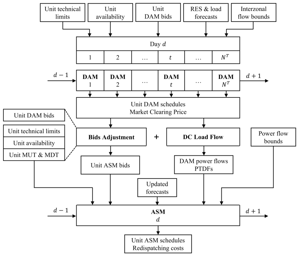
In market-based power systems the ancillary services for the network security can be procured together with energy in a single market session or in a dedicated market downstream the energy procurement [34]. The market process proposed in this work bases its management on the European mechanism involving a multi-stage framework to handle UC and network constraints in the ASM. Particularly, the proposed procedure is composed of four-stages, solved $\forall d\in {\Omega }^D$, as depicted in Figure 2, each one synthesized in the following:

• DAM model: an economic-based merit-order zonal market optimization problem is carried out to define preliminary generation schedules;
• Unit bids adjustment for ASM: a bid adjustment mechanism is carried out to participate to the ASM, based on DAM results, unit technologies and technical limits;
• DCLF and sensitivity factors: a network feasibility analysis of the DAM outcomes is assessed, and the power transfer distribution factors (PTDFs) for the redispatch actions are determined;
• ASM optimization problem: a redispatch procedure that minimizes system costs, with a pay-as-bid mechanism, in the presence of UC and network constraints is employed.

The first stage consists in solving the zonal DAM for each time step t of day d knowing the units’ technical limits, availability and DAM bids. All the units are dispatched according to the economic merit-order, taking into account DA RES and load forecasts, as well as the exchange limits between market zones. This yields a preliminary generation schedule and the Market Clearing Price (MCP). The resulting active power flows are then computed through successive DCLF analyses based on the DAM outcomes, while the cleared bids are adjusted starting from the operating condition defined in the DAM, compatibly with the services that will be offered in the ASM. Once the RES and load forecasts are updated, this latter can be solved for day d.

2.1. DAM Model

The proposed DAM is based on [35] aiming at minimizing step-wise generators bid costs and subject to zonal power flow limits, zonal active power balance, unit maximum bid steps, and generator maximum power in the absence of UC relations. With respect to [35], the thermal unit time-varying maximum power and availability are here considered, along with the DH unit strategy to bid in the DAM. The thermal generator maximum power is determined by means of monthly escalators that consider weather influence on thermal unit rated power and availability due to maintenance, as in (1). The DH unit strategy consists in bidding a certain power amount, lower than maximum available level, in the DAM, with a bidding cost equal to 0 $/MWh, and holding the remaining power amount for the ASM bids.

$$P_{i,t}^{max}=P_i^{max}·e_{i,t}·a_{i,t}$$

(1)

Assuming that load demand is inelastic with respect to price, the DAM is formulated as a linear programming (LP) optimization problem representative of a zonal market. The goal is minimizing the stepwise generation costs at a single time step $t\in {\Omega }^T$ over a time window composed of $N^T$ time steps, each with duration $\tau$. The resulting DAM formulation is stated below:

$$\underset{P_{i,s,t}}{min}\tau ·\sum _{i\in {\Omega }^G}\sum _{s\in {\Omega }_i^S}{c}_{i,s}{P}_{i,s,t}$$

(2)

subject to:

$$P_{i,t}^D=\sum _{s\in {\Omega }_i^S}{P}_{i,s,t},\forall i\in {\Omega }^G$$

(3)

$$0\le P_{i,s,t}\le \Delta P_{i,s,t}^{max},\forall i\in {\Omega }^G,\forall s\in {\Omega }_i^S$$

(4)

$$0\le P_{i,t}^D\le P_{i,t}^{max},\forall i\in {\Omega }^{DT}\cup {\Omega }^{ND}$$

(5)

$$0\le P_{i,t}^D\le P_{i,t}^{da},\forall i\in {\Omega }^R$$

(6)

$$0\le P_{i,t}^D\le k^H{P}_{i,t}^{H,max},\forall i\in {\Omega }^H$$

(7)

$$\sum _{i\in {\Omega }^G}{\alpha }_{i,z}^G{P}_{i,t}^D-\sum _{l\in {\Omega }^L}{\alpha }_{z,l}^F{F}_{l,t}=D_{z,t}^{da},\forall z\in {\Omega }^Z$$

(8)

$$F_l^{lb}\le F_{l,t}\le F_l^{ub},\forall l\in {\Omega }^L$$

(9)

The equality constraint (3) defines the dispatched power of each generator equal to the sum of the cleared bid steps. Inequality (4) limits the power of each bid step within its maximum width. Constraints (5) and (6) are required to ensure that the thermal units never exceed the maximum power and RES never exceed their hourly forecasted power, respectively. For DH units, (7) specifies the maximum power available for each hour according to the dispatch strategy. The zonal active power balance of the system is presented in (8), whereas (9) expresses the active power exchange boundaries on each interzonal connection. In particular, $\Delta P_{i,s,t}^{max}$ is the maximum bid step width, obtained as below:

$$\Delta P_{i,s,t}^{max}=\Delta P_{i,s}^{max}·e_{i,t}$$

(10)

2.2. Unit Bids Adjustment and DCLF Sensitivity Factors

In the framework of distinct energy and service market sessions, the market participants could be called to submit ASM bids prior to the determination of energy market schedules [7]. Therefore, the TSO is called to adjust the submitted bids in order to fit the technical features of the units depending on the closest energy market session results.

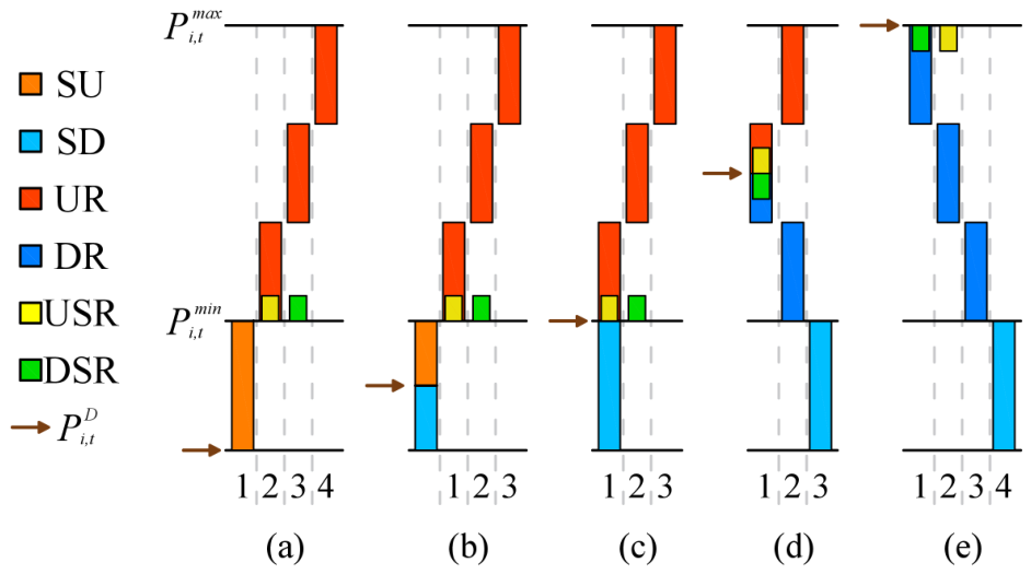
On these bases, the proposed bid adjustment process from TSO perspective is aimed at providing different services depending on DAM schedules and generator technical features, and the economic value of each service is weighted by time-varying factors applied to the DAM bid prices. In particular, the DT units are assumed to provide SU, SD, upward redispatch (UR), downward redispatch (DR), and upward (USR) and downward (DSR) SR services, whereas DH units, equipped with a basin, can only bid UR and DR services, thanks to their higher flexibility and the absence of technical minimum, for each time step t. The bid adjustment process for DT units is described by means of the graphical representation shown in Figure 3, where the numbers represent the clearing order of bids.

In particular, case (a) represents a DT unit not cleared in DAM, and the first bid that could be cleared in ASM is the SU, followed by the first UR step and the USR bids, whereas the DSR bid can be cleared only if the DT unit is above the technical minimum, and the other UR bid steps can be cleared only after using up the previous bid step. Case (b) is similar to case (a); however, the DT unit is cleared below the technical minimum, and the SU bid, up to the technical minimum, or the SD bid, down to zero, must be cleared to comply with the unit constraint. The SU and SD bids are not numbered because the acceptance of one of the two bids is mandatory. Instead, case (c) shows the condition of a DT unit cleared at technical minimum, pointing out the possibility to be shut down, by clearing the SD bid, or to provide upward services, as first action. In case (d) the DT unit is dispatched within its minimum and maximum power levels allowing the unit to clear UR or DR bid along with both SR bids. Finally, in case (e) the unit is cleared at its rated power, hence the first bids that can be cleared are the first DR step and DSR, while the following DR step bids can be cleared only after using up the previous one.

In order to evaluate the power flows ($F_{b,t}^D$) deriving from DAM schedules at each time step t of the considered time horizon, the DCLF procedure is carried out [36]. Moreover, PTDFs ($S_{n,b}$) are calculated to quantify how an incremental change in the nodal active power $\Delta P_n$ affects the branch power flows [37], and to keep generality, PTDFs are calculated by a distributed slack bus DCLF [38], considering all generation nodes as slack buses.

2.3. ASM Optimization Problem

In the nodal ASM optimization problem, assuming TSO viewpoint, the ASM bidding units are redispatched taking into account UC and network constraints to be compliant with SRR procurement and load and RES forecast update. The problem is solved each day over a yearly horizon, composed of $N^D$ days. To this purpose, the objective function $f_d$ aims at minimizing the bid service costs, along with possible load shedding (LS) and RES curtailment (RC) penalties over all time intervals of the day, as follows:

$$f_d=\tau ·{\displaystyle \sum _{t=1}^{N^T}}(C_t^R+C_t^{UD}+C_t^{SR}+C_t^{LS}+C_t^{RC})$$

(11)

where each term of the objective function is defined as:

$$C_t^R=\sum _{i\in {\Omega }^D}\left({\displaystyle \sum _{s=1}^{N_i^S}}{c}_{i,s,t}^{\uparrow }\Delta P_{i,s,t}^{\uparrow }-{\displaystyle \sum _{s=1}^{N_i^S}}{c}_{i,s,t}^{\downarrow }\Delta P_{i,s,t}^{\downarrow }\right)$$

(12)

$$C_t^{UD}=\sum _{i\in {\Omega }^{DT}}\left(C_i^{su}{z}_{i,t}^D{z}_{i,t}^{mu}+c_{i,t}^{su}{P}_{i,t}^{su}{z}_{i,t}^{su}-c_{i,t}^{sd}{P}_{i,t}^{sd}{z}_{i,t}^{sd}\right)$$

(13)

$$C_t^{SR}=\sum _{i\in {\Omega }^{DT}}(c_{i,t}^{sr\uparrow }{P}_{i,t}^{sr\uparrow }-c_{i,t}^{sr\downarrow }{P}_{i,t}^{sr\downarrow })$$

(14)

$$C_t^{LS}=\sum _{n\in {\Omega }^N}{C}^{voll}{D}_{n,t}^{ls}$$

(15)

$$C_t^{RC}=\sum _{i\in {\Omega }^R}{C}^{rc}{P}_{i,t}^{rc}$$

(16)

in which $C_t^R$ is the redispatching cost, $C_t^{UD}$ is the difference between SU and SD costs, $C_t^{SR}$ is the SR provision cost with asymmetric bids. In particular, $C_i^{su}$ is the fixed SU cost, accounted only at first SU time-step through the minimum up time (MUT) binary variable. In addition, $P_{i,t}^{su}$ is the minimum positive value between $P_{i,t}^{min}$ and $P_{i,t}^{min}-P_{i,t}^D$, whereas $P_{i,t}^{sd}$ is the minimum positive value between $P_{i,t}^{min}$ and $P_{i,t}^D$, obtaining $P_{i,t}^{min}$ as in (1) for $P_{i,t}^{max}$.

It has to be noted that from TSO perspective, accepted bids for generation decrease (SD, DR, and SR downward) represent an income for the TSO and are assumed negative in the respective equations, whereas accepted bids for generation increase (SU, UR, and SR upward) are expenses for the TSO, along with LS and RC.

For each $i\in {\Omega }^{DU}$ the DR and UR constraints limit the accepted quantities up to the relevant ASM power bid amount in each step, as in (17) and (18), respectively, whereas (19) allows either UR or DR action:

$$\Delta P_{i,s,t}^{\downarrow }-{\overline{\Delta P}}_{i,s,t}^{\downarrow }{z}_{i,t}^{\downarrow }\le 0,s=1,\dots ,N_i^S$$

(17)

$$\Delta P_{i,s,t}^{\uparrow }-{\overline{\Delta P}}_{i,s,t}^{\uparrow }{z}_{i,t}^{\uparrow }\le 0,s=1,\dots ,N_i^S$$

(18)

$$z_{i,t}^{\uparrow }+z_{i,t}^{\downarrow }\le 1$$

(19)

For each $i\in {\Omega }^{DT}$, the DT unit ASM power redispatch is defined as the algebraic sum of the accepted quantities, except for the SR:

$$\begin{array}{c}\hfill \Delta P_{i,t}^A={\displaystyle \sum _{s=1}^{N_i^S}}\Delta P_{i,s,t}^{\uparrow }-{\displaystyle \sum _{s=1}^{N_i^S}}\Delta P_{i,s,t}^{\downarrow }+P_{i,t}^{su}{z}_{i,t}^{su}-P_{i,t}^{sd}{z}_{i,t}^{sd}\end{array}$$

(20)

Since the bid types and their size and order for the ASM depend on the DAM output, the following DT unit-state constraints are defined taking into account the unit-state due to ASM clearing $\forall t\in {\Omega }^T$:

$$z_{i,t}\le a_{i,t}$$

(21)

$$P_{i,t}^{sr\downarrow }-\Delta P_{i,t}^A\le P_{i,t}^D-P_{i,t}^{min}{z}_{i,t}$$

(22)

$$P_{i,t}^{sr\uparrow }+\Delta P_{i,t}^A\le P_{i,t}^{max}{z}_{i,t}-P_{i,t}^D$$

(23)

$$z_{i,t}^{sr\downarrow }\le z_{i,t}\wedge z_{i,t}^{sr\uparrow }\le z_{i,t}$$

(24)

$$P_{i,t}^{sr\downarrow }-P_i^{sh}{z}_{i,t}^{sr\downarrow }\le 0\wedge P_{i,t}^{sr\uparrow }-P_i^{sh}{z}_{i,t}^{sr\uparrow }\le 0$$

(25)

$$z_{i,t}^{su}\le z_{i,t}\wedge z_{i,t}+z_{i,t}^{sd}\le 1$$

(26)

$${\displaystyle \sum _{t^{\prime }=t}^{t+t_{i,t}^{mu}-1}}{z}_{i,t^{\prime }}\ge t_{i,t}^{mu}{z}_{i,t}^{mu}$$

(27)

$${\displaystyle \sum _{t^{\prime }=t}^{t+t_{i,t}^{md}-1}}(1-z_{i,t^{\prime }})\ge t_{i,t}^{md}{z}_{i,t}^{md}$$

(28)

where, in (21) the unit state is bound by its availability $a_{i,t}$, and it is considered in DAM as well. The minimum and maximum power constraints are defined in (22) and (23), respectively, where the units can provide the SR only if they have suitable upward or downward margins. With (24), upward and downward SR can be bid only by active DT, respectively, whereas (25) limit the downward and upward SR provision up to the unit SRH. In (26), the unit state is consequent to SU and SD cleared bids, respectively, i.e., if the DT unit is started up in ASM it has to be $z_{i,t}=1$, whereas if the DT unit is shut down it yields $z_{i,t}=0$. DT units are subject by MUT and minimum down time (MDT) constraints, respectively, modelled in (27) and (28), where $t_{i,t}^{mu}$ ($t_{i,t}^{md}$) is the minimum between the unit MUT (MDT) and the remaining time steps of the day as defined below:

$$t_{i,t}^{mu}=min\{M{U}_i,N^T-t\};t_{i,t}^{md}=min\{M{D}_i,N^T-t\}$$

(29)

Constraints (30)–(34) explicitate the conditions of all cases illustrated in Figure 3, and their activation depends on the DAM schedule $P_{i,t}^D$. If it is below $P_{i,t}^{min}$, the unit is forced in (30) to firstly clear the SU bid before the UR ones, as in the conditions (a) and (b); moreover, if it is not null the unit must clear either SU bid or SD bid in (31), this condition is depicted in (b). If the DAM schedule is greater than $P_{i,t}^{min}$, in (32) the SU bid cannot be cleared—as in the conditions (c)–(e)—whereas if the DAM schedule is null, in (33) the SD bid cannot be cleared, as in (a). Instead, in (34) the SD bid can be accepted only if all the DR bids are cleared, reaching the minimum power, as in the conditions (d) and (e).

$$z_{i,t}^{\uparrow }\le z_{i,t}^{su}\mathrm{if}{P}_{i,t}^D<P_{i,t}^{min}$$

(30)

$$z_{i,t}^{su}+z_{i,t}^{sd}=1\mathrm{if}0<P_{i,t}^D<P_{i,t}^{min}$$

(31)

$$z_{i,t}^{su}=0\mathrm{if}{P}_{i,t}^D\ge P_{i,t}^{min}$$

(32)

$$z_{i,t}^{sd}=0\mathrm{if}{P}_{i,t}^D=0$$

(33)

$${\displaystyle \sum _{s=1}^{N_i^S}}{\overline{\Delta P}}_{i,s,t}^{\downarrow }{z}_{i,t}^{sd}\le {\displaystyle \sum _{s=1}^{N_i^S}}\Delta P_{i,s,t}^{\downarrow }\mathrm{if}{P}_{i,t}^D>P_{i,t}^{min}$$

(34)

Although the optimization problem is solved on a daily horizon, MUT and MDT constraints introduce inter-temporal dependencies on i-th DT unit. Specifically, if a unit is turned on (off) during the ending hours of day $d-1$, it could still be under MUT (MDT) constraint at the beginning of day d.

To enforce constraint continuity between days, two auxiliary parameters are introduced downstream the ASM solution of the day $d-1$, named $t_{i,d-1}^{on}$ and $t_{i,d-1}^{off}$, representing the number of consecutive time steps with $z_{i,t}=1$ and $z_{i,t}=0$, respectively, from the last time-step of the day $d-1$. The conditional constraint provided in Algorithm 1 is defined based on d and t, linking $t_{i,d-1}^{on}$ with $M{U}_i$ and $t_{i,d-1}^{off}$ with $M{D}_i$. This ensures that $z_{i,t}^{mu}$, $z_{i,t}^{md}$, and $z_{i,t}$ are either fixed to specific values or related through an additional constraint.

Algorithm 1 MUT & MDT Continuity Algorithm

1: Set $d\leftarrow {\Omega }^D$   2: for  $i=1,\dots ,N^{DT}$  do   3:      Set $t_{i,d-1}^{on},t_{i,d-1}^{off},M{U}_i,M{D}_i\leftarrow {\Omega }^{DT}$   4:      for $t=1,\dots ,N^T$ do   5:            if $t_{i,d-1}^{on}=0$ then   6:               if $t_{i,d-1}^{off}<M{D}_i\wedge t<M{D}_i-t_{i,d-1}^{off}$ then   7:                    $z_{i,t}=z_{i,t}^{mu}=z_{i,t}^{md}=0$   8:               else   9:                    $z_{i,t}^{mu}-z_{i,t}^{md}=z_{i,t}-z_{i,t-1}$ 10:               end if 11:            else if $t_{i,d-1}^{off}=0$ then 12:               if $t_{i,d-1}^{on}<M{U}_i\wedge t<M{U}_i-t_{i,d-1}^{on}$ then 13:                    $z_{i,t}=1\wedge z_{i,t}^{mu}=z_{i,t}^{md}=0$ 14:               else 15:                    $z_{i,t}^{mu}-z_{i,t}^{md}=z_{i,t}-z_{i,t-1}$ 16:               end if 17:            end if 18:      end for 19: end for

For the sake of clarity, consider a unit with $M{U}_i=4$ and $t_{i,d-1}^{on}=2$, hence the unit is operating since the last two hours of the day $d-1$ and it must operate for 2 more hours at d. Therefore, at $t=$ 1 and $t=$ 2, $z_{i,t}=1$ and $z_{i,t}^{mu}=z_{i,t}^{md}=0$, whereas for the rest of the day the unit can keep operating or can be shut down.

An additional inter-temporal dependency involves the programmed availability of the i-th DT unit at day $d+1$ and its MUT constraints at ending hours of the day d. To ensure constraint consistency between MUT at d and availability at $d+1$ a further auxiliary parameter is introduced upstream the ASM solution named $a_{i,d+1}^{re}$ which counts the $a_{i,t}=1$ at $d+1$ from the beginning of the day up to the first $a_{i,t}=0$. The implemented rule, provided in Algorithm 2, relates $a_{i,d+1}^{re}$ and $M{U}_i$ to fix $z_{i,t}^{mu}=0$. For example, if the i-th DT unit has $a_{i,d+1}^{re}=2$ and $M{U}_i=4$, the unit can be started up to $t=23$ of d to make MUT compliant with its availability at $d+1$.

Algorithm 2 MUT & Availability Continuity Algorithm

1: Set $d\leftarrow {\Omega }^D$ 2: for  $i=1,\dots ,N^{DT}$  do 3:       Set $a_{i,d+1}^{re},M{U}_i\leftarrow {\Omega }^{DT}$ 4:       if $a_{i,d+1}^{re}<M{U}_i$ then 5:           for $t=24,\dots ,24-(M{U}_i-a_{i,d+1}^{re}+1)$ do 6:                 $z_{i,t}^{mu}=0$ 7:           end for 8:       end if 9: end for

For the DH units, the constraints (17)–(19) are still valid, whereas (20) is modified eliminating SU and SD terms. Specific DH unit constraints are, $\forall i\in {\Omega }^H$ and $\forall t\in {\Omega }^T$:

$$E_i^{lb}\le E_{i,t}^{av}-\tau \Delta P_{i,t}^A\le E_i^{ub}$$

(35)

$$-P_{i,t}^D\le \Delta P_{i,t}^A\le min\{P_i^{max}-P_{i,t}^D,(E_i^{ub}-E_{i,t}^{av})/\tau \}$$

(36)

$$z_{i,t}^{ns}{E}_i^{ub}/\tau \le {\displaystyle \sum _{s=1}^{N_i^S}}\Delta P_{i,s,t}^d+E_{i,t-1}^{av}/\tau$$

(37)

The energy balance is limited in (35) within the upper and the lower boundaries of the DH basin, (36) defines the limits of the total DH redispatched power, where the maximum power is the minimum between the available energy over the time interval and the upper power margin, whereas the minimum power is the opposite of the DAM schedule. The DH unit stops storing energy when the sum of the available energy and the DR power reaches the upper bound as in (37). At each time step t, $E_{i,t}^{av}$ is updated according to the initial available energy ($E_{i,0}^{av}$), the inlet energy ($E_{i,t}^M$) and the DAM schedules up to the actual time step t, and the ASM cleared bids until the time step $t-1$ as follows:

$$\begin{array}{c}\hfill E_{i,t}^{av}=E_{i,0}^{av}+{\displaystyle \sum _{\widehat{t}=1}^t}(E_{i,\widehat{t}}^M-\tau P_{i,\widehat{t}}^D)-{\displaystyle \sum _{\widehat{t}=1}^{t-1}}\tau \Delta P_{i,\widehat{t}}^A\end{array}$$

(38)

The RC and LS are limited to an upper bound defined as:

$$0\le P_{i,t}^{rc}\le P_{i,t}^{rt},\forall i\in {\Omega }^R$$

(39)

$$0\le D_{n,t}^{ls}\le D_{n,t}^{rt},\forall n\in {\Omega }^N$$

(40)

Finally, network constraints are:

$$\begin{array}{c}\hfill \sum _{i\in {\Omega }^D}[P_{i,t}^D+\Delta P_{i,t}^A]+\sum _{i\in {\Omega }^{ND}}{P}_{i,t}^D+\sum _{i\in {\Omega }^R}[P_{i,t}^{rt}-P_{i,t}^{rc}]=\sum _{n\in {\Omega }^N}[D_{n,t}^{rt}-D_{n,t}^{ls}],\forall n\in {\Omega }^N\end{array}$$

(41)

$$F_b^{lb}\le F_{b,t}^D+\Delta F_{b,t}\le F_b^{ub},\forall b\in {\Omega }^B$$

(42)

$$\begin{array}{cc}\hfill \Delta F_{b,t}& =\sum _{n\in {\Omega }^N}{S}_{n,b}\left(\sum _{i\in {\Omega }^D}{\beta }_{i,n}\Delta P_{i,t}^A+\sum _{i\in {\Omega }^R}{\beta }_{i,n}\Delta P_{i,t}^R-\right.\hfill \\ \hfill & \left.-\Delta D_{n,t}^L+D_{n,t}^{ls}-\sum _{i\in {\Omega }^R}{\beta }_{i,n}{P}_{i,t}^{rc}\right),\forall b\in {\Omega }^B\hfill \end{array}$$

(43)

$$\sum _{i\in {\Omega }^{DT}}{P}_{i,t}^{sr\downarrow }=SR{R}_t\wedge \sum _{i\in {\Omega }^{DT}}{P}_{i,t}^{sr\uparrow }=SR{R}_t$$

(44)

where (41) represents the power balance of the system, (42) limits the branches power flow up to the upper or lower bound, neglecting interzonal limitations in accordance with the ASM nodal approach, (43) defines the power flow variation according to the PTDF, the redispatched quantities, the curtailed resources, and the forecast update of load demand and of non-dispatchable RES productions, whereas (44) defines the UR and DR SR amounts to be procured. Particularly, since the DR SR is an income for the TSO, the equality constraint is required for the SR to avoid an over-reservation.

3. Test System Features

The proposed methodology is applied to the NREL-118 Bus System which includes datasets of load demand and WF and PV production for a leap year with hourly resolution ($N^T=$ 8784), along with costs, availability and escalators of the generation mix, and monthly energy availability of the DH units [31,39]. The generation set consists of 327 units for a total installed capacity of 40.5 GW, composed of 11.0 GW combined cycle (CC), 3.6 GW combustion turbine (CT), 2.5 GW steam turbine (ST), 10.2 GW non dispatchable hydroelectric, 8.5 GW DH, 1.0 GW WF, and 3.4 GW of PV, and the remaining is distributed among internal combustion engine (ICE), biomass (Bio), and geothermal (Geo) technologies.

The rated power of DT and DH units is supposed equal to or greater than 10 MW. Therefore, 89 DT are involved in the ASM, as reported in

Table 1. DT unit parameters.

Technology	n.	${\mathit{P}}_{\mathit{i}}^{\mathit{min}}$ [MW]	${\mathit{P}}_{\mathit{i}}^{\mathit{max}}$ [MW]	${\mathit{c}}_{\mathit{i},\mathit{s}}$ [$/MW]	${\mathit{C}}_{\mathit{i}}^{\mathit{su}}/{\mathit{P}}_{\mathit{i}}^{\mathit{max}}$ [$/MW]	MUT [h]	MDT [h]
CC NG	28	[4.1, 503.9]	[13.5, 943.5]	[24.5, 61.3]	[83.6, 83.7]	[2, 6]	[2, 8]
CT NG	47	[4.5, 81.0]	[15.0, 180.0]	[27.9, 65.7]	[33.9, 109.2]	[1, 8]	[1, 8]
CT Oil	5	[21.4, 22.4]	[71.2, 74.5]	[192.3, 242.3]	31.8	2	2
Geo	1	11.0	22.0	2.7	0	6	6
ST NG	8	[8.5, 57.0]	[106.3, 712.0]	[43.1, 60.0]	79.5	8	12

, where per each technology and fuel–natural gas (NG) and oil–the total number, the $P_i^{min}$, the $P_i^{max}$ along with the steps costs $c_{i,s}$ and the specific SU fixed cost $C_i^{su}/P_i^{max}$ are reported, and the $P_i^{sh}$ is supposed the 6% of $P_i^{max}$.

Moreover, 15 DH units are individuated, and in

Table 2. DH unit parameters.

		DH Basin Features		DH Inlet Energy
DH	${\mathit{P}}_{\mathit{i}}^{\mathit{max}}$ [MW]	${\mathit{E}}_{\mathit{i}}^{\mathit{lb}}$ [MWh]	${\mathit{E}}_{\mathit{i}}^{\mathit{ub}}$ [GWh]	Daily Min [h/d]	Daily Max [h/d]	Yearly [h/y]
1–2	75.0	300	12.60	1.44 (November)	7.13 (May)	1701.1
3–4	77.0	308	12.94	2.53 (November)	10.14 (May)	2517.2
5	82.0	328	13.78	0.30 (February)	7.09 (June)	842.1
6–10	1225.3	4901	205.85	2.13 (March)	15.08 (July)	2797.2
11–12	810.8	3243	136.21	0.59 (January)	8.84 (May)	1476.2
13	46.7	187	7.85	2.14 (September)	3.75 (May)	1139.9
14	110.0	440	18.48	1.51 (November)	12.56 (May)	2314.3
15	140.0	560	23.52	1.92 (November)	15.98 (May)	2945.5

, $P_i^{max}$, the features of DH basin ($E_i^{ub}$ and $E_i^{lb}$) and the inlet energy are described.

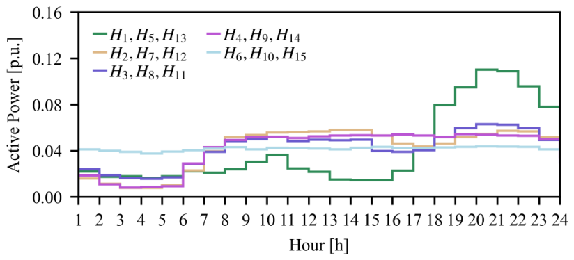
For DH units, the 90% of the daily inlet energy is bid to the DAM, where the hourly quantity of the submitted bids follow five different behaviours as shown in Figure 4, based on [40], the remaining 10% is held for the ASM. For the elaboration of UR and DR bid prices in Section 2, an equivalent DAM price bid is supposed to equal the daily median value of the DAM zonal price of the pertaining market zone.

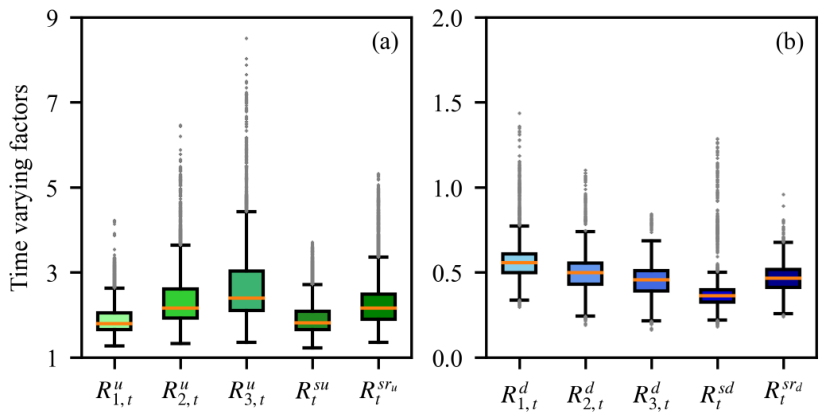
The time-varying factors of the bid adjustment process are shown in Figure 5a and Figure 5b for the selling and buying bids, respectively. They have been obtained by processing the hourly Italian market bids, thanks to the similarity of system features in terms of RES impact and the analogous multi-stage market structure by averaging the hourly ratio between the ASM bid prices of each service and the DAM step prices submitted by each market participant [41]. It has to be noticed that, as expectable in a pay-as-bid framework, the selling ASM prices are greater than the selling DAM ones (i.e., time-varying factors for UR, SU, and positive SR are greater than 1), in order to make ASM power increase more profitable, whereas the buying ASM prices are mainly lower than the selling DAM ones (i.e., time-varying factors for DR, SD and negative SR are lower than 1), since the buying bids represent an expense for the market participants that should be lower than the marginal production price to ensure a revenue. These average hourly values are therefore assigned to each dispatchable unit considering a gaussian variation with 99.7% confidence interval set at 10% of the value.

In order to allow the activation of RC and LS actions as last resources, the values of $C^{rc}$ and $C^{voll}$ are high enough to represent the most expensive services representing a cost in the objective function, as follows:

$$C^{rc}=max\left(c_{i,s,t}^{\uparrow }\right)+10$$

(45)

$$C^{voll}=max\left({\displaystyle \frac{C_i^{su}}{P_i^{min}}}\right)+10$$

(46)

The load forecast error between DAM and ASM is taken from zonal load [31] and split among nodes through participation factors, whereas RES errors are treated separately for each PV units and WFs. The maximum, minimum, and average errors of each resource are reported in

Table 3. Maximum, minimum, and average forecast error values [MW].

	Load	PV	WF	NFE
Max	2987.90	500.82	411.95	3312.48
Min	−3654.28	−1223.80	−391.00	−3667.76
Avg	55.33	−70.01	−15.88	141.21

, noting that load error reaches roughly 10% of peak load, whereas error on PV and WF can reach roughly 40% of installed power. In Table 3, the analogous values for the net forecast error (NFE), defined as the difference in each time interval between total load error and total RES errors, are reported as well.

4. Result Analyses

The whole framework is implemented in Python (v. 3.10)-based environment where the DAM and ASM optimizations are developed by means of Pyomo library [42] using Gurobi solver [43] and DIgSILENT PowerFactory is employed for the DCLF and sensitivity analysis, exploiting the Python API to automatize the simulation process. Simulations are performed on a computer with 32 GB RAM, 12th Gen Intel^® Core™ i9-12900F CPU @ 2.40 GHz, 16 physical cores, and 24 logical processors, using up to 24 threads. The daily process is averagely solved within 4 min, where the ASM solution represents the highest computational burden with an average elapsed time by roughly 2.5 min, in line with the time requirements of SCADA/EMS systems.

4.1. Elaboration of ASM Inputs

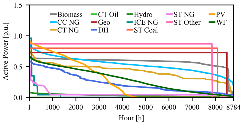
The generation schedules yielded by DAM solution, normalized for each technology installed capacity, are reported in Figure 6. CC NG technology is most frequently called to produce due to lower production cost, providing 51.48 TWh during the year, followed by DH and CT NG supplying 16.98 TWh and 12.20 TWh, respectively. The total RES contribution amounts to 31.2%, (i.e., 30.00 TWh). ST NG and ICE NG turn out to cover the demand peaks, due to higher DAM bid prices. Some technologies have constant escalators at low price therefore, quite constant power levels are observed. The DAM zonal prices over the year are reported in

Table 4. DAM zonal prices in $/MWh.

	Zone	Zone 1	Zone 2	Zone 3
Value
Maximum		54.72	54.72	54.72
Average		34.75	34.74	34.74
Minimum		27.02	27.02	27.02

. Negligible differences among market zones are observed, due to sporadic interzonal congestions (56 occurrences on Zone 1-Zone 2).

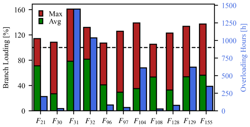
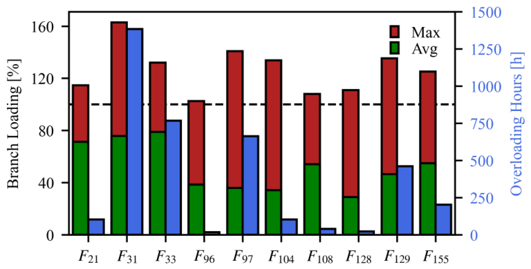
The DCLF outcomes show that 11 branches experience DAM overloads, as reported in Figure 7. These are most frequent in branches 31 and 32 since they are close to the most convenient units. Further overloads are detected on contiguous lines 96, 97, and 104.

The SRR values are determined as in [44], and range from 94.4 MW to 302.5 MW according to load demand. The upward (downward) SR margin, USM (DSM), is the sum of the minimum value between the SRH and the upward (downward) margin of each cleared DT unit after DAM solution. During the year, the DSM is sufficient to cover the SRR, whereas for 741 time steps the USM is lower than the SRR, which, in turn, requires SU or DR bid clearances in ASM to fulfil the constraint (44).

4.2. Yearly ASM Results

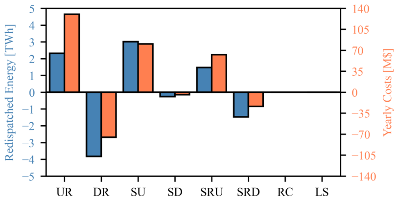
The NCUCER yearly costs and the redispatched amounts per each service are shown in Figure 8. The yearly TSO disbursement (obtained by summing the objective function (11) over the year) is equal to USD 170.2 M due to the higher costs for upward actions with respect to revenues for downward ones. Since the dispatchable units are able to provide the services required by the network, without curtailing any RES production or shedding any load consumption, the system adequacy is proved. It has to be noted that the most cleared amounts are DR and SU bids, since the former is a revenue for the TSO, whereas the latter is cheaper than UR bids.

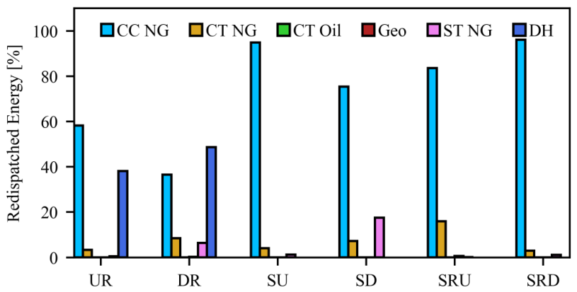
The contributions of each generation technology to service provision are depicted in Figure 9. It can be stated that CC NG technology is the most exploited thanks to its economic viability, followed by the DH for the UR and DR services. On the other hand, CT NG technology is marginally cleared, mainly providing SRU service due to its higher cost and greater upward and downward availability. Finally, ST NG are mostly cleared for SU and SD due to higher costs.

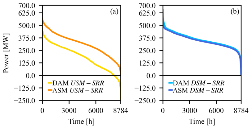
Regarding the SRR fulfillment, Figure 10a shows the difference between USM and SRR after DAM and ASM, and analogously in Figure 10b for the difference between DSM and SRR. It can be observed that DSM is enough to cover SRR and a very slight variation from DAM to ASM is registered. On the contrary, USM in ASM is increased due to SU and DR clearance, to create a suitable margin to be compliant with SRR constraint, i.e., the illustrated difference is always non-negative.

The number of cleared SU and SD bids in the whole year, for each technology, is reported in

Table 5. Yearly number of occurrences of SU and SD.

Technology	Total SU	Total SD	Total Activation of (31)	of Which SU	of Which SD
CC NG	28,206	1718	1820	1412	408
CT NG	6176	1200	339	99	240
ST NG	1448	962	64	5	59

. It can be noted that the occurrences in which (31) is activated, mainly to comply with UC feasibility, represent a quarter of the yearly horizon. Since CC NG represents the most recurrent marginal technology in DAM over year, its SU bid is cleared for three quarter of (31) activation occurrences. Comparing with technologies, the higher SU costs of CT NG and ST NG units imply a greater occurrence of SD with respect to SU.

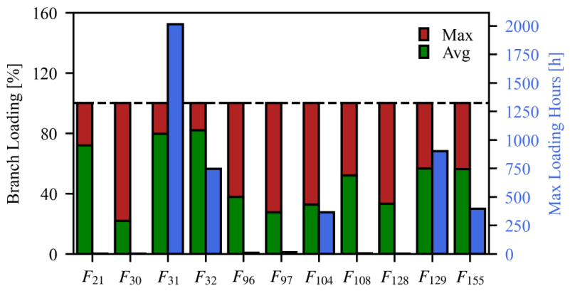
After ASM, the overloads experienced on the 11 branches are all solved within the maximum loading, as reported in Figure 11. When comparing with Figure 7, the maximum loading after ASM is experienced for less hours with respect to DAM overloads, for all branches, except for $F_{31}$ and $F_{129}$ due to the clearance of cheapest units with a concordant PTDF with the branch flows.

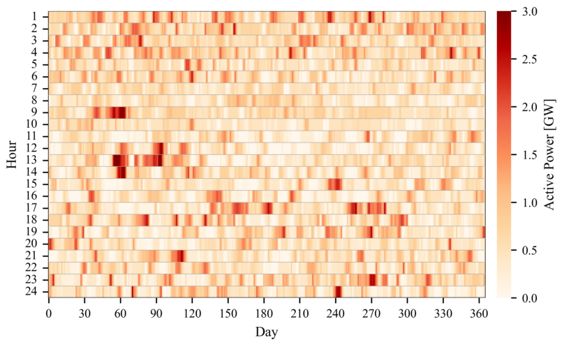
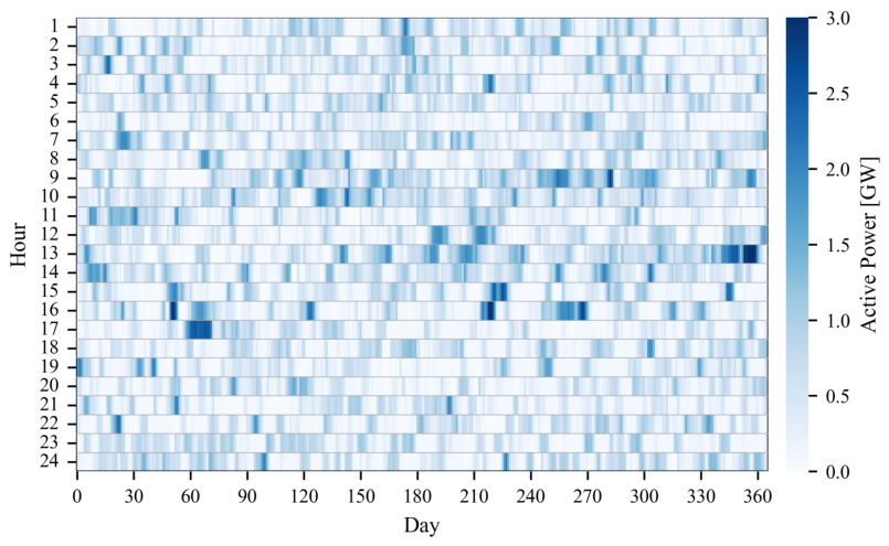
The heat maps depicted in Figure 12 and Figure 13 provide the yearly profile of the total upward and downward redispatched energy, respectively, highlighting the hours of the days with highest and lowest movements. In particular, from Figure 12 can be inferred that in weeks 9 (days 57–63) and 2 (days 8–14) the highest and lowest upward cleared amount are stated, amounting to 98.5 GWh and 55.1 GWh, respectively. Instead, from Figure 13 it can be observed that in weeks 43 (days 295–301) and 15 (days 99–105) the highest and lowest downward cleared amount occur, accounting for 98.5 GWh and 55.1 GWh, respectively.

4.3. Weekly ASM Results with the Most Redispatched Energy

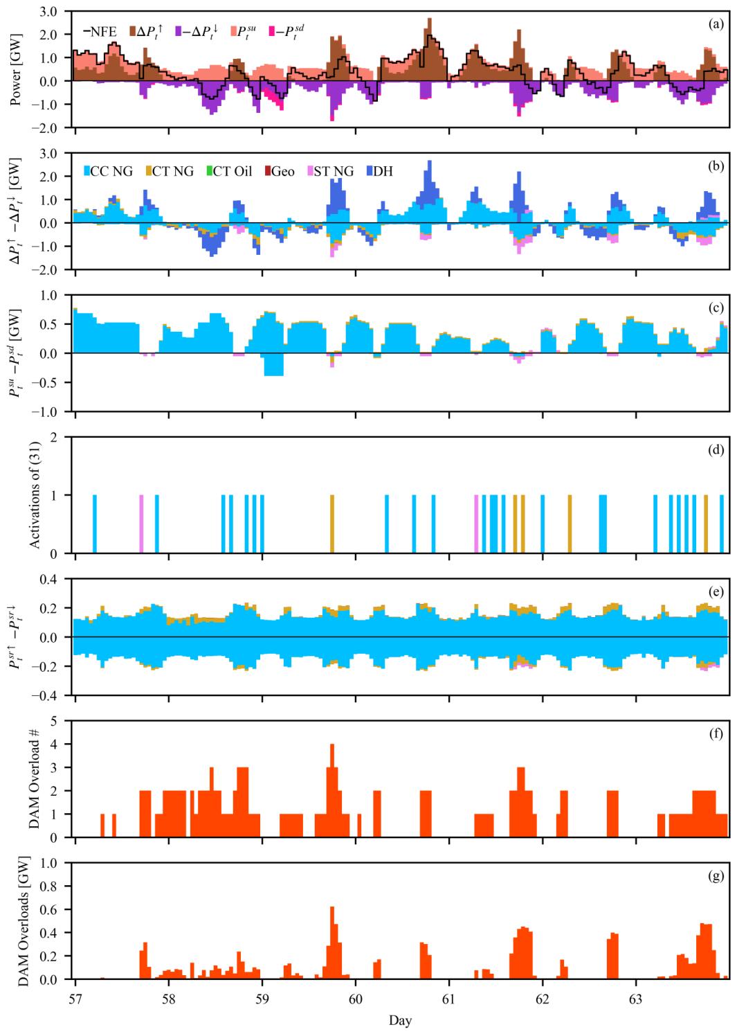
In addition to the yearly analysis, the results depicted in Figure 14 show the details of week 9 with the highest redispatched energy among all services, accounting for 210.2 GWh. In particular, Figure 14a depicts the hourly NFE along with the total cleared amounts of UR, DR, SU, and SD, observing some intervals with total redispatched amount greater than the NFE due to the need for mitigation of network or units constraints.

Particularly, in Figure 14b and Figure 14c the UR and DR and the SU and SD cleared amounts are provided, respectively per technology, remarking the economic driver of the ASM, since the most expensive units are mainly called to reduce their production or to be shut down. In particular, ST NG units are mainly shut down due to great MUT and MDT values, CT NG SU bids are cleared only with positive NFE, whereas CC NG are shut down only with negative NFE lasting longer than their MDT value. However, some SU and SD cleared bids depend on the activation of (31), as highlighted in Figure 14d, observing that only for the CC NG the SU bid is cleared even for negative NFE. This technological feature is mirrored in SRR provision as well, observing in Figure 14e that ST NG provides the downward SR only in the hours with a cleared amount in DAM, while fulfilling the MUT. Finally, Figure 14f and Figure 14g depict the DAM overloaded line number and power, respectively, stating that the hours with the greatest redispatched power require overloads mitigation, whereas the hours with a redispatch slightly higher than the NFE are present to comply with MUT and MDT constraints.

4.4. Sensitivity Analysis on ASM Bid Factors and DH Bidding Strategy

In order to provide insight on the influence of specific aspects on the model performance, a set of sensitivities is carried out.

A first sensitivity analysis considers ASM bid prices, with two cases on time-varying factors, in particular a simulation with larger prices increasing the selling bid time-varying factors by 10% while decreasing the buying bid time-varying factors by 10%, magnifying the variation w.r.t. DAM bids, and a simulation with narrower prices with opposite variation, reducing the difference from DAM bids. The objective function outcomes are provided in

Table 6. Sensitivity on ASM bid factors. Yearly service provision and costs.

ASM Service	Base Case		Narrower Prices				Larger Prices
	Power [TWh]	Cost [M$]	Power [TWh]	Cost [M$]	$\mathbf{\Delta }$P [%]	$\mathbf{\Delta }$$ [%]	Power [TWh]	Cost [M$]	$\mathbf{\Delta }$P [%]	$\mathbf{\Delta }$$ [%]
UR	2.315	130.20	2.301	116.19	−0.6	−10.8	2.304	162.85	−0.5	+9.7
DR	3.822	75.22	4.223	90.91	+10.5	+20.9	3.496	62.46	−8.5	−17.0
SU	3.016	88.05	3.429	81.79	+13.7	−7.1	2.686	82.75	−10.9	−6.0
SD	0.268	4.13	0.265	4.81	−1.1	+16.5	0.253	3.42	−5.6	−17.2
SRU	1.470	62.56	1.470	53.93	0.0	−13.8	1.470	71.16	0.0	+13.7
SRD	1.470	23.78	1.470	26.13	0.0	+10.9	1.470	21.43	0.0	−9.9

along with the base case yields. The provided UR amount is almost unaffected by the price variation, and this could infer that UR service is mainly cleared to mitigate line overloads. On the contrary, the other services are affected by price variation, resulting in greater cleared quantities with narrower prices, being more convenient for the TSO, and lower market movements with larger prices, being more expensive for the TSO.

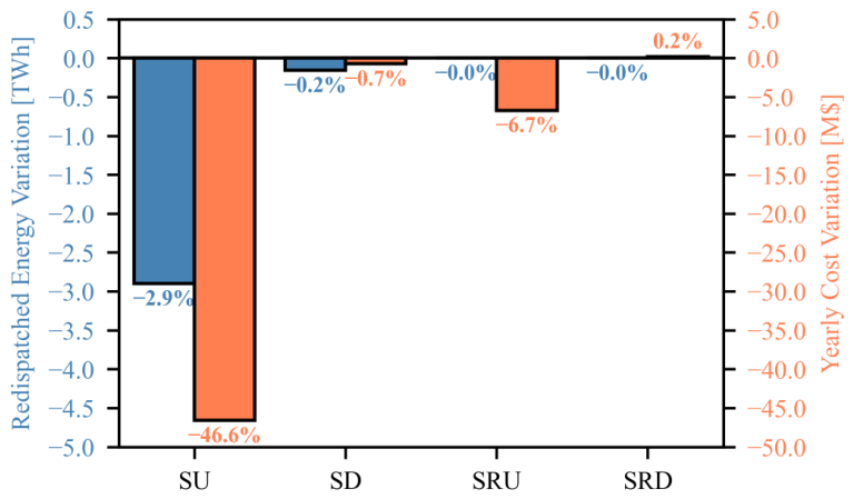
Moreover, to assess the relevance of the bidding strategy by DH, a new strategy is tested, where 85% of the daily inlet energy is bid to the DAM and the remaining 15% is held for the ASM. As a result, DH production in DAM is reduced by roughly 0.94 TWh over the year. CC NG covers roughly 72.7% of this energy, mainly employing units installed in same market zone of DH, previously limited by interzonal congestions, reduced to 36 occurrences. In fact, the maximum, average and minimum zonal prices are roughly increased by 1%, as shown by the prices provided in

Table 7. DAM zonal price with 85% of Hydro energy bid in USD/MWh.

	Zone	Zone 1	Zone 2	Zone 3
Value
Maximum		55.58	55.58	55.58
Average		34.99	34.99	34.99
Minimum		27.41	27.41	27.41

.

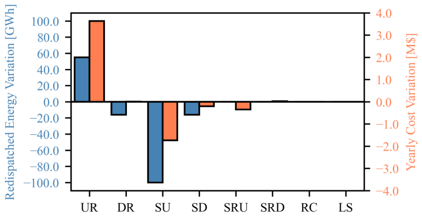
The DCLF with the new generation profiles yielded the same branches affected by overloads; however, the total occurrences increased from 4517 to 4537 and the greatest overload obtained on $F_{31}$ is increased to 161.5%, implying more UR for mitigation. The redispatched energy and cost variation, depicted in Figure 15, show an increase of UR clearing by roughly 55 GWh, whereas DR, SU and SD energies are all decreased. Particularly, the great reduction of SU is ascribable to the higher number of cleared units in DAM, able to directly provide SR avoiding unit startings. Regarding the overall costs, the TSO expense is increased by roughly USD 1.72 M, mainly due to the UR provision by more expensive DT units.

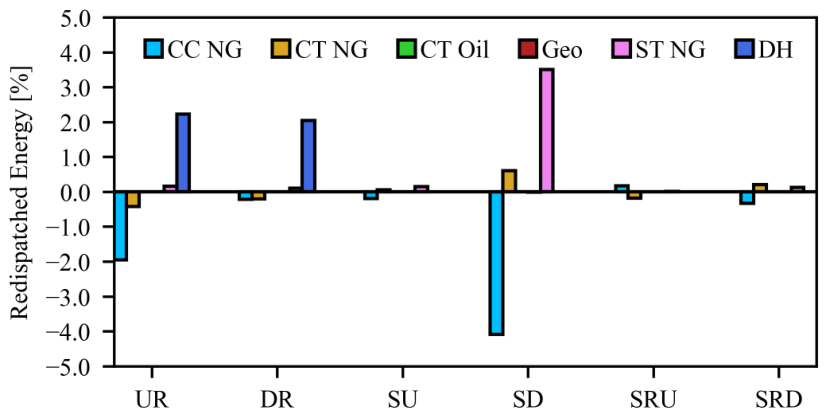
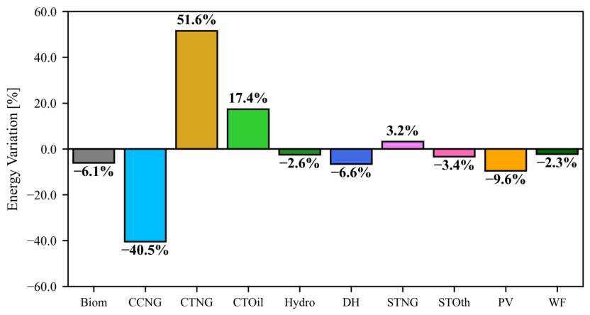
The variations of the contributions of each technology to service provision are depicted in Figure 16. The greater DH unit availability in ASM makes the CC NG contribution to UR reduce by roughly 2%, whereas for DR the DH units have greater prevalence to mitigate local network overloads. The DAM clearance of costly ST NG units implies their wider use for SD service in the place of cheaper CC NG.

4.5. Comparison with Benchmark DAM Model

The proposed approach is compared with a benchmark DAM model with UC and reserve provision, based on [32] including MUT and MDT constraints as in [33] along with Algorithms 1 and 2 to ensure feasibility among days, keeping the zonal market framework. Its formulation is provided in Appendix A, and analogies with constraints of the proposed DAM-ASM framework are pointed out. The average simulation time of the benchmark model is 2 min/day, roughly halving the time consumption of the proposed approach but not considering forecast updates and nodal redispatch.

The benchmark model provides 56 congestions as well; however, as reported in

Table 8. Benchmark model DAM zonal prices in USD/MWh.

	Zone	Zone 1	Zone 2	Zone 3
Value
Maximum		242.27	242.27	242.27
Average		199.25	199.39	199.39
Minimum		45.21	45.21	45.21

, the maximum, average, and minimum zonal prices are roughly 5, 6, and 2 times greater than the base case reported in Table 4. This is ascribable to the necessity of keeping start-up a due number of DT units to fulfill the SR provision, being the SRH limited to the 6% of DT unit maximum power. This can be inferred by the dispatched energy variation depicted in Figure 17. In particular, in the proposed DAM model, CC NG units are cleared up to the maximum power, as well as non-dispatchable units. Instead, in the benchmark model, CC NG units cannot provide the maximum power to comply with USR constraints, and more expensive units—i.e., CT NG, CT Oil, and ST NG—are cleared above the technical minimum in order to reach the required amount of both DSR and USR margins, involving a reduction of cleared bids of units with null bid price.

The higher energy costs imply a reduction of SU costs of DT units along with the SRU provision as can be observed in Figure 18. Specifically, only 115.0 GWh of SU occurs over the year resulting in USD 34.0M of expense and this implies smaller SD actions. Despite the SRU and SRD amounts being unvaried, the cleared DT units to provide the service are cheaper allowing savings of USD 6.93M. However, comparing the overall cost of DAM energy along with SU, SD, SRU, and SRD service costs, the proposed approach provides an expense of USD 3.49B against the USD 19.50B of the benchmark model (i.e., 5.6 times smaller). Additionally, downstream the DAM with UC and reserve constraints, DCLF simulations are carried out and relevant outcomes are depicted in Figure 19 observing a lower amount of overloaded lines (10) and occurrences (3755) w.r.t. the base case, though arising the need of nodal redispatch for their mitigation, with consequent costs not included in the benchmark.

5. Conclusions

In this paper, a NCUCER optimization problem has been employed to efficiently redispatch power from zonal DAM to nodal ASM to meet load and RES forecast updates complying with UC and network constraints, according to the European approach. The sequential interaction of the two markets has been managed with a bid adjustment process for ASM to fit the units’ technical limits with respect to the DAM schedules. The proposed procedure has proved to successfully handle RES variability, unit state constraints, and network requirements (e.g., SRR or overloads) with a reasonable computational burden. The developed approach provides a useful tool for evaluating the services needed by the TSOs to comply with the security requirements of the system. Sensitivity analysis has demonstrated the strategies on bid escalators and DH availability most affecting ASM outcomes. Furthermore, compared to benchmark market model with UC and reserve constraints, the proposed approach allows a reduction in the total costs thanks to greater flexibility for starting-up or shutting-down units depending on the contingency, i.e., overload mitigation, SR provision, or NFE mitigation.

The tool could be a promising solution for ASM participants with relevant information levels: the TSO could derive indications about network criticalities and total occurred costs, whereas generation companies could evaluate bidding strategies able to satisfy both network service requirements and operating points. The proposed approach, framing zonal DAM-nodal ASM interaction as in European context, could be applicable to different systems, providing the needed inputs (e.g., marginal costs, network parameters, bid factors).

Possible future work could deal with the provision of tertiary reserve services into NCUCER optimization, as well as security-constrained approach. Furthermore, the framework could be extended by adopting stochastic or robust optimization techniques to better hedge against load and RES uncertainties. Finally, the integration of emerging flexibility resources, such as Energy Storage Systems and demand-side management, represents a key step to further enhance the economic efficiency and security of the proposed methodology.

References

1. Poplavskaya, K.; Joos, M.; Krakowski, V.; Knorr, K.; de Vries, L. Redispatch and balancing: Same but different. Links, conflicts and solutions. In Proceedings of the 2020 17th International Conference on the European Energy Market (EEM), Stockholm, Sweden, 16–18 September 2020; pp. 1–6. [Google Scholar] [CrossRef] [Scilit]
2. ENTSO-E. Cross Border Electricity Balancing Pilot Projects. 2026. Available online: https://eepublicdownloads.entsoe.eu/clean-documents/Network%20codes%20documents/Implementation/Pilot_Projects/151130_Report_P9.pdf (accessed on 21 February 2026).
3. All NEMO Committee. Single Day-Ahead Coupling (SDAC). 2026. Available online: https://www.nemo-committee.eu/sdac (accessed on 17 February 2026).
4. All NEMO Committee. Single Intraday Coupling (SIDC). 2026. Available online: https://www.nemo-committee.eu/sidc (accessed on 19 February 2026).
5. ENTSO-E. Electricity Balancing. 2026. Available online: https://www.entsoe.eu/network_codes/eb/ (accessed on 21 January 2026).
6. Domínguez, R.; Oggioni, G.; Smeers, Y. Reserve procurement and flexibility services in power systems with high renewable capacity: Effects of integration on different market designs. Int. J. Electr. Power Energy Syst. 2019, 113, 1014–1034. [Google Scholar] [CrossRef] [Scilit]
7. Gestore Mercati Energetici (GME). Spot Market MPE. Available online: https://www.mercatoelettrico.org/en-us/Home/Markets/ElectricityMarket/Spot-Market-MPE#MGP (accessed on 29 September 2025).
8. Yang, N.; Dong, Z.; Wu, L.; Zhang, L.; Shen, X.; Chen, D.; Zhu, B.; Liu, Y. A Comprehensive Review of Security-constrained Unit Commitment. J. Mod. Power Syst. Clean Energy 2022, 10, 562–576. [Google Scholar] [CrossRef] [Scilit]
9. Tsegaye, S.; Shewarega, F.; Bekele, G. A Review on Security Constrained Economic Dispatch of Integrated Renewable Energy Systems. EAI Endorsed Trans. Energy Web 2020, 8, e13. [Google Scholar] [CrossRef] [Scilit]
10. Pitto, A.; Cirio, D.; Ciapessoni, E. Probabilistic security-constrained preventive redispatching in presence of correlated uncertainties. In Proceedings of the 2020 AEIT International Annual Conference (AEIT), Catania, Italy, 23–25 September 2020; pp. 1–6. [Google Scholar] [CrossRef] [Scilit]
11. Fan, M.; Huang, L. Generator Redispatch Control Strategy with Big Data for Power Systems with Renewable Energy. In Proceedings of the 2019 IEEE Power & Energy Society General Meeting (PESGM), Atlanta, GA, USA, 4–8 August 2019; pp. 1–5. [Google Scholar] [CrossRef] [Scilit]
12. Yu, Z.; Zhong, H.; Ruan, G.; Yan, X. Network-Constrained Unit Commitment With Flexible Temporal Resolution. IEEE Trans. Power Syst. 2025, 40, 73–84. [Google Scholar] [CrossRef] [Scilit]
13. Mende, D.; Stock, D.S.; Hennig, T.; Löwer, L.; Hofmann, L. Multiobjective optimization in congestion management considering technical and economic aspects. In Proceedings of the 2016 IEEE PES Asia-Pacific Power and Energy Engineering Conference (APPEEC), Xi’an, China, 25–28 October 2016; pp. 1061–1066. [Google Scholar] [CrossRef] [Scilit]
14. Klabunde, C.; Wolter, M. Mixed Integer Linear Programming Time-Series Based Redispatch Optimization. In Proceedings of the 2020 IEEE PES Innovative Smart Grid Technologies Europe (ISGT-Europe), The Hague, The Netherlands, 26–28 October 2020; pp. 504–508. [Google Scholar] [CrossRef] [Scilit]
15. Morales, J.M.; Conejo, A.J.; Perez-Ruiz, J. Economic Valuation of Reserves in Power Systems With High Penetration of Wind Power. IEEE Trans. Power Syst. 2009, 24, 900–910. [Google Scholar] [CrossRef] [Scilit]
16. Silva Pinto, M.S.; Pinto, M.S.S.; Saavedra, O.R. Power Reserve Dispatch to Mitigate Variability of Generation Output due to Wind Ramps. In Proceedings of the 2020 IEEE PES Transmission & Distribution Conference and Exhibition—Latin America (T&D LA), Montevideo, Uruguay, 28 September–2 October 2020; pp. 1–6. [Google Scholar] [CrossRef] [Scilit]
17. Abdelmalak, M.; Benidris, M. Proactive Generation Redispatch to Enhance Power System Resilience During Hurricanes Considering Unavailability of Renewable Energy Sources. IEEE Trans. Ind. Appl. 2022, 58, 3044–3053. [Google Scholar] [CrossRef] [Scilit]
18. Münz, U.; Mesanovic, A. Optimal redispatch and primary reserve allocation for power systems with uncertain load and generation. In Proceedings of the 2016 European Control Conference (ECC), Aalborg, Denmark, 29 June–1 July 2016. [Google Scholar] [CrossRef] [Scilit]
19. García-González, J.; Roque, A.M.S.; Campos, F.A.; Villar, J. Connecting the Intraday Energy and Reserve Markets by an Optimal Redispatch. IEEE Trans. Power Syst. 2007, 22, 2220–2231. [Google Scholar] [CrossRef] [Scilit]
20. IEEE Power & Energy Society. Security Constrained Unit Commitment for Electricity Market: Modeling, Solution Methodology and Future Challenges; Technical Report PES-TR96; IEEE Power & Energy Society: Piscataway, NJ, USA, 2022. [Google Scholar] [CrossRef]
21. De Tuglie, E.; Dicorato, M.; La Scala, M.; Scarpellini, P. Dynamic security preventive control in a deregulated electricity market. In Proceedings of the PSCC 1999, Trondheim, Norway, 28 June–2 July 1999; pp. 125–131. [Google Scholar]
22. Nycander, E.; Morales-España, G.; Söder, L. Capacity and Intra-Hour Ramp Reserves for Wind Integration. IEEE Trans. Sustain. Energy 2022, 13, 1430–1443. [Google Scholar] [CrossRef] [Scilit]
23. Goudarzi, H.; Rayati, M.; Sheikhi, A.; Ranjbar, A.M. A clearing mechanism for joint energy and ancillary services in non-convex markets considering high penetration of renewable energy sources. Int. J. Electr. Power Energy Syst. 2021, 129, 106817. [Google Scholar] [CrossRef] [Scilit]
24. Aguilar, J.; Bordons, C.; Arce, A. Chance Constraints and Machine Learning integration for uncertainty management in Virtual Power Plants operating in simultaneous energy markets. Int. J. Electr. Power Energy Syst. 2021, 133, 107304. [Google Scholar] [CrossRef] [Scilit]
25. Reddy, S.S.; Bijwe, P.; Abhyankar, A. Optimum day-ahead clearing of energy and reserve markets with wind power generation using anticipated real-time adjustment costs. Int. J. Electr. Power Energy Syst. 2015, 71, 242–253. [Google Scholar] [CrossRef] [Scilit]
26. Liu, X.; Conejo, A.J. Day-ahead reserve determination in power systems with high renewable penetration. Int. J. Electr. Power Energy Syst. 2024, 156, 109703. [Google Scholar] [CrossRef] [Scilit]
27. Charbonnier, F.; Morstyn, T.; McCulloch, M.D. Coordination of resources at the edge of the electricity grid: Systematic review and taxonomy. Appl. Energy 2022, 318, 119188. [Google Scholar] [CrossRef] [Scilit]
28. Rancilio, G.; Rossi, A.; Falabretti, D.; Galliani, A.; Merlo, M. Ancillary services markets in europe: Evolution and regulatory trade-offs. Renew. Sustain. Energy Rev. 2022, 154, 111850. [Google Scholar] [CrossRef] [Scilit]
29. Honkapuro, S.; Jaanto, J.; Annala, S. A Systematic Review of European Electricity Market Design Options. Energies 2023, 16, 3704. [Google Scholar] [CrossRef] [Scilit]
30. Falvo, M.C.; Panella, S.; Caprabianca, M.; Quaglia, F. A Review on Unit Commitment Algorithms for the Italian Electricity Market. Energies 2022, 15, 18. [Google Scholar] [CrossRef] [Scilit]
31. Peña, I.; Martinez-Anido, C.B.; Hodge, B.M. An Extended IEEE 118-Bus Test System With High Renewable Penetration. IEEE Trans. Power Syst. 2018, 33, 281–289. [Google Scholar] [CrossRef] [Scilit]
32. Conejo, A.J.; Baringo, L. Unit commitment and economic dispatch. In Power System Operations; Springer International Publishing AG: Cham, Switzerland, 2017; pp. 197–232. [Google Scholar]
33. Morales-España, G.; Tejada-Arango, D.A. Modeling the hidden flexibility of clustered unit commitment. IEEE Trans. Power Syst. 2019, 34, 3294–3296. [Google Scholar] [CrossRef] [Scilit]
34. Shah, D.; Chatterjee, S. A comprehensive review on day-ahead electricity market and important features of world’s major electric power exchanges. Int. Trans. Electr. Energy Syst. 2020, 30, e12360. [Google Scholar] [CrossRef] [Scilit]
35. Tricarico, G.; Wagle, R.; Dicorato, M.; Forte, G.; Gonzalez-Longatt, F.; Rueda, J.L. Zonal Day-Ahead Energy Market: A Modified Version of the IEEE 39-bus Test System. In Proceedings of the 2022 IEEE PES Innovative Smart Grid Technologies—Asia (ISGT Asia), Singapore, 1–5 November 2022; pp. 86–90. [Google Scholar] [CrossRef] [Scilit]
36. Stott, B. Review of load-flow calculation methods. Proc. IEEE 1974, 62, 916–929. [Google Scholar] [CrossRef] [Scilit]
37. Ronellenfitsch, H.; Timme, M.; Witthaut, D. A Dual Method for Computing Power Transfer Distribution Factors. IEEE Trans. Power Syst. 2017, 32, 1007–1015. [Google Scholar] [CrossRef] [Scilit]
38. Exposito, A.; Ramos, J.; Santos, J. Slack bus selection to minimize the system power imbalance in load-flow studies. IEEE Trans. Power Syst. 2004, 19, 987–995. [Google Scholar] [CrossRef] [Scilit]
39. Dicorato, M.; Tricarico, G.; Forte, G.; Marasciuolo, F. Technical Indicators for the Comparison of Power Network Development in Scenario Evaluations. Energies 2021, 14, 4179. [Google Scholar] [CrossRef] [Scilit]
40. Comanescu, D.; Grigoras, G.; Cartina, G.; Rotaru, F. Determination of typical load profiles in hydro-power plant by clustering techniques. In Proceedings of the 2010 12th International Conference on Optimization of Electrical and Electronic Equipment, Brasov, Romania, 20–22 May 2010; pp. 1294–1297. [Google Scholar] [CrossRef] [Scilit]
41. Gestore Mercati Energetici (GME). Public Domain Bids. Available online: https://www.mercatoelettrico.org/en-us/Home/Results/Electricity/MSD/ExAnte/Download/Download?valore=OffertePubbliche (accessed on 14 September 2023).
42. Hart, W.E.; Laird, C.D.; Watson, J.P.; Woodruff, D.L.; Hackebeil, G.A.; Nicholson, B.L.; Siirola, J.D. Pyomo-Optimization Modeling in Python; Springer Nature: Cham, Switzerland, 2017; Volume 67. [Google Scholar]
43. Gurobi Optimization. 2026. Available online: https://www.gurobi.com (accessed on 25 November 2025).
44. Tricarico, G.; Dicorato, M.; Forte, G.; Gonzalez-Longatt, F. Contributions to Tertiary Reserve Requirements under Operating Conditions and Uncertainties. In Proceedings of the 2022 18th International Conference on the European Energy Market (EEM), Ljubljana, Slovenia, 13–15 September 2022; pp. 1–6. [Google Scholar] [CrossRef] [Scilit]
Figure 1. Italian market framework and main features.
Energies 19 02377 g001
Figure 2. Workflow of the proposed procedure to model DAM/ASM sequential interaction.
Energies 19 02377 g002
Figure 3. Bids’clearing order: not cleared unit (a), unit cleared below the technical minimum (b), unit cleared at the technical minimum (c), unit cleared between the technical limits (d), unit cleared at the rated power (e).
Energies 19 02377 g003
Figure 4. DH daily power bid profiles.
Energies 19 02377 g004
Figure 5. Selling (a) and buying (b) bid time-varying factors boxplots.
Energies 19 02377 g005
Figure 6. DAM dispatched power duration curve.
Energies 19 02377 g006
Figure 7. Branches overloads after DAM.
Energies 19 02377 g007
Figure 8. Yearly costs and redispatched energy.
Energies 19 02377 g008
Figure 9. Services provided for each technology.
Energies 19 02377 g009
Figure 10. SRR and USM difference between DAM and ASM (a) and SRR and DSM difference between DAM and ASM (b).
Energies 19 02377 g010
Figure 11. Loading after ASM of branches overloaded in DAM.
Energies 19 02377 g011
Figure 12. Yearly heatmap of UR + SU cleared amounts.
Energies 19 02377 g012
Figure 13. Yearly heatmap of DR + SD cleared amounts.
Energies 19 02377 g013
Figure 14. Results of the week 9. Hourly NFE and total cleared amounts (a), UR and DR by technology (b), SU and SD by technology (c), activations of (31) (d), SRR provision by technology (e), DAM overloaded lines (f), DAM overload power (g).
Energies 19 02377 g014
Figure 15. ASM redispatched energy and cost variation with 85% of DH energy bid in DAM.
Energies 19 02377 g015
Figure 16. Services provision variation for each technology with 85% of DH energy bid in DAM.
Energies 19 02377 g016
Figure 17. Benchmark model. Yearly dispatched energy variation w.r.t. the proposed model.
Energies 19 02377 g017
Figure 18. Benchmark model. Yearly SU, SD, SRU, and SRD energy and cost variations w.r.t. the proposed model.
Energies 19 02377 g018
Figure 19. Benchmark model. Branches overloads in UC with reserve DAM.
Energies 19 02377 g019