Crude Oil Prices Forecasting in the Energy Transition Era: Evidence from Geopolitical and Technological Drivers

Abstract

This study examines crude oil return dynamics in the context of the global energy transition, where decarbonization policies, technological innovation, and shifting energy demand increasingly influence market behavior. We propose a heavy-tailed distributional LSTM framework to jointly model the conditional mean, volatility, and tail risk of West Texas Intermediate (WTI) returns, incorporating key transition-related drivers: carbon allowance returns (ETS), artificial intelligence (AI) activity, electric vehicle (EV) market returns (SPKS), and geopolitical risk (GPR). Granger causality results show that ETS significantly predicts mean returns, reflecting the growing impact of climate policy signals, while AI and EV markets primarily affect volatility, indicating transmission through uncertainty channels. The model adopts a Student-t specification to capture heavy-tailed behavior and extreme price movements. Out-of-sample results reveal limited mean predictability but improved forecasting of return magnitude and tail risk. These findings highlight that, under energy transition dynamics, oil market predictability is increasingly concentrated in the risk dimension rather than in average returns.

1. Introduction

The global energy system is undergoing a profound structural transformation driven by decarbonization policies, technological innovation, and shifting demand patterns. This ongoing energy transition is progressively reshaping the role of fossil fuels, including crude oil, within the global economy. Despite this transition, crude oil remains a strategically critical commodity, influencing inflation, production costs, trade balances, financial stability, and geopolitical dynamics [1,2,3]. However, the determinants of oil price dynamics are no longer confined to traditional supply–demand fundamentals. Instead, they increasingly reflect the interaction between fossil fuel markets and transition-related forces such as climate policy, electrification, and technological change [4,5,6].

Within this evolving landscape, oil markets are becoming embedded in a broader environment, shaping expectations. The acceleration of electric vehicle (EV) adoption, the expansion of carbon pricing mechanisms, and the rapid development of artificial intelligence (AI) are altering both current market behavior and expectations about future energy demand. For instance, the rapid growth of EV markets signals long-term substitution away from oil in transportation, while carbon markets embed policy-driven constraints on carbon-intensive activities. At the same time, AI-related technological expansion influences energy consumption patterns and investment allocation, particularly through increased electricity demand and industrial transformation [7,8]. These developments imply that oil price formation must be analyzed within the broader context of energy transition dynamics rather than as an isolated commodity market phenomenon.

From a theoretical standpoint, traditional oil price models emphasize demand shocks, supply disruptions, precautionary demand, and inventory behavior [1,9]. While these mechanisms remain relevant, they are increasingly complemented, and sometimes dominated, by transition-driven channels. Carbon allowance markets (ETS), for example, affect oil prices by altering the relative cost of fossil fuel use, transmitting climate policy expectations, and influencing fuel substitution decisions [10]. Similarly, geopolitical risk continues to play a central role, but its interaction with transition dynamics can amplify uncertainty, particularly in a fragmented global energy system [11]. In this context, oil markets exhibit heightened sensitivity not only to physical shocks but also to policy signals, financial flows, and technological expectations.

These structural changes have important implications for forecasting. Crude oil price series are typically non-stationary, exhibiting trends, structural breaks, and time-varying variance [12]. To address this issue, empirical studies commonly transform prices into returns, which are generally stationary and more suitable for econometric modeling [13]. However, even when stationarity is achieved in the mean, crude oil returns still exhibit important stylized facts, including nonlinearity, volatility clustering, and heavy-tailed distributions [14]. These features imply that standard linear models may be insufficient to capture the full dynamics of oil markets, particularly under conditions of heightened uncertainty and structural change [15]. Traditional forecasting approaches, which often focus on conditional mean prediction, are therefore insufficient for capturing the full risk profile of oil markets. In the context of an energy transition, understanding volatility dynamics and tail risks is particularly important, as extreme price movements may arise from abrupt policy shifts, technological breakthroughs, or geopolitical disruptions. Consequently, a distributional perspective that jointly models expected returns, volatility, and tail behavior becomes essential for both financial and policy applications.

Against this background, this study examines whether key energy transition-related and uncertainty-driven variables, namely AI activity, carbon allowance returns (ETS), geopolitical risk (GPR), and EV market returns (SPKS), contain predictive information for crude oil return dynamics. Specifically, the study aims to (i) assess the extent to which these factors influence the conditional mean and volatility of oil returns; (ii) distinguish between directional predictability and risk-based transmission channels; and (iii) develop a forecasting framework capable of capturing the distributional properties of oil returns in a transition-driven environment.

This paper contributes to the literature in several ways. First, it situates crude oil forecasting explicitly within the energy transition paradigm by integrating technological, environmental, and geopolitical drivers into a unified framework. Second, it advances the understanding of heterogeneous transmission mechanisms by distinguishing between mean and volatility/tail-risk predictability. Third, it adopts a heavy-tailed distributional LSTM approach that jointly models return dynamics and risk characteristics, addressing the limitations of traditional point-forecasting methods. Finally, the study provides practical insights into risk management and energy policy by identifying which transition-related variables are most relevant for forecasting oil market behavior under structural change.

The choice of West Texas Intermediate (WTI) crude oil as the benchmark in this study is motivated by both theoretical and practical considerations. WTI is one of the most widely traded and liquid crude oil benchmarks globally, serving as a key reference price in financial markets and academic research. Its high frequency of trading and deep derivatives market make it particularly suitable for modeling return dynamics and volatility behavior. Moreover, WTI reflects market conditions in a major oil-producing region and is extensively used in forecasting studies, allowing comparability with the existing literature. From an econometric perspective, the availability of high-quality, continuous data and its responsiveness to both global and regional shocks make WTI an appropriate proxy for analyzing the interaction between oil markets and energy transition drivers. Therefore, its selection ensures both empirical robustness and consistency with prior research.

The remainder of the paper is organized as follows. Section 2 reviews the literature. Section 3 presents the methodology, including data construction, variable definitions, preliminary predictive-content testing, and the proposed heavy-tailed distributional LSTM framework. Section 4 describes the experimental design, training configuration, benchmarks, and evaluation metrics. Section 5 reports and discusses the empirical results for mean forecasting, magnitude/volatility forecasting, and heavy-tail dynamics. Section 6 concludes with implications for energy economics and finance, limitations, and directions for future research.

2. Materials and Methods

The energy forecasting challenge is exacerbated by the fact that oil markets exhibit strong nonlinearity, volatility clustering, structural breaks, and sensitivity to geopolitical and policy shocks, which often undermine the effectiveness of standard linear predictive models [16,17,18]. In this context, the literature has evolved from traditional econometric specifications toward machine learning, deep learning, and hybrid systems that aim to better capture the complex dynamics of the oil market.

2.1. Systematic Literature Review

A systematic literature review (SLR) offers a structured and transparent synthesis of recent advances in crude oil forecasting, enhancing rigor and reproducibility through a defined search and selection protocol that reduces bias [19]. Covering studies ranging from 2020 to 2026, it focuses on machine learning, deep learning, and energy transition–related forecasting [19]. Searches in Scopus, Web of Science, and Google Scholar used keywords such as “crude oil forecasting,” “machine learning,” “deep learning,” “energy transition,” “carbon markets,” “geopolitical risk,” and “volatility forecasting” [20]. Studies were carefully screened for relevance, rigor, and empirical contribution [21], with inclusion criteria requiring crude oil forecasting, econometric/ML/hybrid methods, and integration of exogenous drivers [22]. The final sample was classified into econometric, ML/DL, and hybrid frameworks [21], revealing a shift toward nonlinear, data-driven models with greater emphasis on external risk factors and volatility dynamics [23]. Yet, limited work has jointly modeled the full conditional distribution of oil returns with energy transition variables [24], motivating the present study’s adoption of a distributional LSTM to capture both return dynamics and risk comprehensively.

Table 1. Recent Oil Forecasting and Energy-Market Studies.

Study	Period/ Market	Method	Key Variables	Main Contribution/ Finding	Relevance to this Study
[25]	Crude oil	LSTM with optimization	Oil prices	LSTM improves nonlinear crude oil forecasting accuracy.	Supports use of deep learning.
[26]	Crude oil	Traditional forecasting models	Oil prices	Econometric models remain useful benchmarks but face limits under instability.	Supports benchmark discussion.
[27]	Oil futures	Deep learning with news sentiment	Sentiment, oil returns, volatility	Sentiment improves return and volatility forecasting.	Supports exogenous information channels.
[28]	Carbon price	Hybrid time-series + LS-SVM	Carbon prices	Hybrid models improve forecasting by combining statistical and ML methods.	Supports carbon-market relevance.
[22]	Crude oil	ML models + Google search data	Search data, oil price	External information improves crude oil forecasting.	Supports multi-factor design.
[29]	Crude oil	Hybrid GRU with decomposition	Oil prices	Decomposition–deep learning improves forecasting stability.	Supports nonlinear sequential modeling.
[30]	Crude oil	Interval forecasting with textual data	Climate text, oil prices	Climate-related textual information improves oil-price interval forecasts.	Links climate information to oil forecasting.
[31]	Fossil and clean energy	DCC-GARCH	Fossil energy, clean energy, major assets	Finds dynamic volatility links among fossil and clean energy markets.	Supports volatility-spillover argument.
[32]	Energy commodities	Hybrid deep learning	Economic policy uncertainty, energy prices	Uncertainty improves energy commodity forecasting.	Supports uncertainty-based predictors.
[18]	Crude oil	Deep forest ensemble	Oil prices	Ensemble ML captures nonlinear oil-price dynamics.	Supports advanced ML alternatives.
[21]	Crude oil	ML with variable selection	Multivariate predictors	Predictor selection improves crude oil forecasting performance.	Supports exogenous feature selection.
[33]	Crude oil	iTransformer hybrid model	Risk factors, oil prices	Risk-factor screening improves early warning of crude oil fluctuations.	Supports risk-factor integration.
[34]	Energy markets	Nonlinear energy-market analysis	Geopolitical risk	GPR has nonlinear and state-dependent energy-market effects.	Supports inclusion of GPR.
[35]	New energy, carbon, oil	Spillover analysis	New energy, carbon markets, crude oil	Finds spillovers between new energy, carbon markets, and oil.	Supports ETS and EV-market inclusion.
[36]	Crude oil futures	ML methods	Energy uncertainty index	Energy uncertainty improves crude oil futures forecasting.	Supports uncertainty and transition predictors.

summarizes key recent contributions, highlighting model types, datasets, and main findings.

Table 1 reveals several patterns in recent crude oil forecasting research. First, methods have shifted from traditional econometrics to ML/DL approaches to better capture nonlinear dependencies and complex temporal structures. Second, incorporating exogenous variables leads to a substantial improvement in performance. Third, studies increasingly highlight energy market interconnectedness, documenting spillovers between oil, carbon, and clean energy sectors, especially under stress. Yet most work still emphasizes point-forecast accuracy, with limited attention to full conditional distributions. Moreover, transition-related drivers are often examined in isolation rather than within unified frameworks. Addressing this gap, the present study employs a multi-factor design with a heavy-tailed distributional LSTM to jointly model mean, volatility, and tail risk in crude oil returns.

2.2. Box–Jenkins Framework and Time-Series Modeling Foundations

Traditional crude oil forecasting often relies on the Box–Jenkins methodology, which models stochastic processes through ARIMA specifications [37]. It involves three steps: model identification, parameter estimation, and diagnostic checking, with the key requirement that the series be stationary [38]. Since oil prices are typically non-stationary and subject to structural breaks, transformations such as differencing or returns are used [12], though these may sacrifice long-run information. ARIMA models capture linear dependence and short-memory dynamics, making them useful baselines, but their assumptions of linearity and constant parameters limit their ability to address nonlinearities, structural changes, and exogenous interactions [39]. These limitations become more critical under energy transition dynamics, where oil market behavior is increasingly shaped by climate policy, technological change, and geopolitical uncertainty. [40]. Thus, while Box–Jenkins remains a benchmark, it is insufficient for modern oil markets, motivating nonlinear and data-driven approaches such as the distributional LSTM proposed here.

2.3. Traditional Econometric Forecasting Models and Their Limitations

Traditional econometric forecasting models rely on linear dependence structures and stable parameter assumptions. Early studies widely applied ARIMA, VAR, and GARCH specifications for their interpretability and ability to capture serial dependence and conditional heteroskedasticity [26,41]. These remain useful benchmarks for short-memory processes and volatility persistence, but their performance weakens during crises, regime shifts, and nonlinear transitions such as COVID-19 or geopolitical shocks [42]. Their emphasis on constant parameters and mean prediction overlooks oil markets’ time-varying interactions, asymmetric shocks, and cross-market dependencies [43,44]. Even GARCH models, though effective for volatility clustering, struggle with heavy-tailed returns and nonlinear exogenous drivers [44,45]. As a result, these frameworks struggle under uncertainty, policy changes, and technological disruption, prompting the use of nonlinear, data-driven methods like machine learning and deep learning for crude oil forecasting.

2.4. Machine Learning and Deep Learning Advances in Crude Oil Forecasting

Machine learning (ML) and deep learning (DL) models approximate complex nonlinear functions without restrictive parametric assumptions, making them well-suited for financial time series where relationships are nonlinear, time-varying, and multi-factor. Recent work shows strong progress in crude oil forecasting, with ANN, LSTM, GRU, and CNN outperforming traditional models in capturing hidden patterns and adapting to nonstationary environments [25,29]. Advanced architectures such as TCNs and recurrent hybrids also deliver strong results for WTI and Brent, though performance depends on features, horizon, and market conditions [20,29]. Hybrid designs, like GARCH-LSTM or GRU systems [46], and iTransformer frameworks with risk-factor screening further enhance accuracy and early warning under volatility and structural breaks [33]. Yet no single model dominates; outcomes hinge on feature design and regime conditions. Consequently, modern oil forecasting increasingly relies on flexible, data-driven frameworks that integrate heterogeneous information, positioning DL approaches as particularly effective for markets shaped by uncertainty, structural change, and energy transition dynamics.

2.5. Hybrid and Decomposition-Based Frameworks

Another strand of research emphasizes hybrid models that combine signal decomposition with ML/DL predictors. Since crude oil prices contain latent components, long-term trends, cycles, and high-frequency noise, methods like EMD, ensemble EMD, and VMD are used to isolate these before prediction, improving learning efficiency and pattern detection [28,29,47]. By separating frequency components, decomposition reduces noise and enhances model performance, especially in markets shaped by overlapping shocks and structural changes. Integrated with neural networks or other predictors, these hybrids consistently improve accuracy, as decomposition strengthens signal quality while ML captures nonlinear dependencies [48]. They are particularly effective under volatility clustering and abrupt events, though most remain focused on point metrics (RMSE, MAE) and neglect distributional features such as heavy tails and tail risk [32]. Given the importance of extreme price movements in energy markets, this gap motivates the present study’s distributional approach to capture both point forecasts and the full return distribution.

2.6. Exogenous Predictors and Multi-Factor Forecasting Design

A growing body of research shows that crude oil forecasting improves when exogenous variables are incorporated alongside autoregressive information. Oil markets are embedded in macro-financial and geopolitical systems, so relying solely on past prices risks omitted variable bias. Empirical studies explore predictors such as macroeconomic indicators, exchange rates, financial variables, uncertainty indices, commodity signals, and sentiment proxies [21,22], which capture demand expectations, financial conditions, and global risk sentiment. Uncertainty-related variables are especially prominent; for example, Wei et al. illustrate that an energy-related uncertainty index enhances forecasting across horizons [36]. With the energy transition, uncertainty from policy, technology, and global conditions becomes central. To manage large predictor sets, methods like LASSO, PCA, and risk-factor screening are used to reduce overfitting and improve robustness [33,41,49]. Yet most studies treat exogenous variables in isolation, underscoring the need for unified multi-factor frameworks that integrate macroeconomic, financial, technological, and policy drivers. The present study addresses this gap by embedding transition-related and uncertainty-driven variables within a nonlinear, distributional forecasting framework to better capture crude oil return dynamics.

2.7. Sentiment, Oil, and New Technology Determinants

Behavioral finance highlights that oil prices are shaped not only by fundamentals but also by sentiment, attention, and expectations. Investors often react to news and narratives before macroeconomic indicators adjust, motivating the use of sentiment proxies such as search behavior, news text, and social media signals in forecasting models [30,50]. Empirical evidence shows these variables improve short-term forecasts, especially under informational frictions [27,51]. Parallel research emphasizes oil’s interconnectedness with carbon and clean energy markets, documenting spillovers and asymmetric transmissions during crises like COVID-19 and geopolitical conflicts [35,52,53]. Geopolitical risk (GPR) further exerts nonlinear, state-dependent effects, with stronger impacts in high-volatility regimes [34]. Yet, studies often remain fragmented—analyzing carbon, GPR, and new-energy assets separately [10,54,55,56], or focusing on spillovers rather than direct forecasting [31,53]. Moreover, AI is typically treated as a tool rather than a determinant of oil dynamics [57,58]. These gaps underscore the need for a unified nonlinear framework integrating transition-related and uncertainty-driven variables, which the present study aims to provide.

2.8. From Point Forecasting to Distributional Forecasting: The Remaining Gap

From a financial economics perspective, modeling only the conditional mean is inadequate when return distributions exhibit heavy tails, excess kurtosis, and time-varying volatility, features well documented in crude oil returns [59]. Point-forecast frameworks relying on RMSE or MAE fail to capture the full risk profile, which is critical for investment, hedging, and policy in energy markets [60]. Despite advances in ML, DL, and hybrid approaches, most studies still emphasize accuracy over distributional properties and tail-risk behavior [20]. Yet modern oil markets are increasingly shaped by geopolitical uncertainty, energy transition, and cross-market interactions, all of which affect dispersion and extreme outcomes [61]. A distributional framework is therefore essential to jointly model mean, volatility, and higher-order moments [60]. To address this gap, the present study combines a multi-factor design (AI, ETS, GPR, SPKS variables) with a heavy-tailed distributional LSTM to capture nonlinear dependencies and tail behavior comprehensively. Overall, the literature review highlights three key insights: (i) the limitations of linear models in capturing nonlinear oil market dynamics, (ii) the growing importance of exogenous and transition-related variables, and (iii) the need for distributional forecasting approaches. These insights directly inform the methodological design of the present study.

3. Data Description and Preliminary Analysis

Before model estimation, preliminary statistical analysis is conducted to understand the properties of the data. To assess stationarity, Augmented Dickey–Fuller (ADF) tests are performed. The results confirm that all return series are stationary at conventional significance levels, justifying their use in the predictive framework. Additionally, correlation analysis is conducted to examine linear dependencies between variables. While correlations remain moderate, nonlinear dependencies may still exist, motivating the use of deep learning models.

Table 2. Descriptive Statistics of Return Series.

Variable	Mean	Std. Dev.	Min	Max	Skewness	Kurtosis	IQR (Q3–Q1)
WTI	0.0003	0.0215	−0.1450	0.1280	−0.42	6.85	0.024
ETS	0.0004	0.0182	−0.1100	0.1020	0.35	5.72	0.020
GPR	0.0001	0.0256	−0.1620	0.1750	0.88	7.94	0.030
AI	0.0006	0.0191	−0.0950	0.1100	0.27	4.96	0.021
SPKS	0.0005	0.0223	−0.1300	0.1400	0.51	6.10	0.026

reports summary statistics, including mean, standard deviation, skewness, and kurtosis for all variables.

The descriptive statistics highlight key features of the data. All return series show small mean values, consistent with financial returns, while standard deviations, especially for WTI and GPR, indicate substantial variability. Skewness reveals asymmetry, with GPR and SPKS positively skewed and WTI slightly negative. Crucially, all variables exhibit excess kurtosis, confirming heavy-tailed distributions. The interquartile range (IQR) further underscores dispersion and extreme observations. These stylized facts justify the use of nonlinear and distributional modeling approaches in the subsequent analysis. In addition to standard descriptive statistics, the skewness and kurtosis values indicate that all variables deviate from normality. Positive kurtosis values confirm leptokurtic distributions, while skewness suggests asymmetry in return behavior. Furthermore, interquartile range (IQR) analysis reveals the presence of significant outliers, particularly during periods of market stress, supporting the need for robust modeling approaches.

3.1. Stationarity and Time-Series Properties

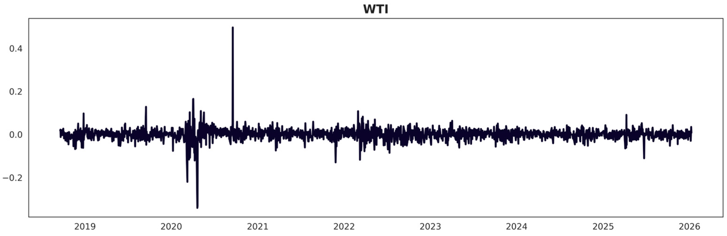
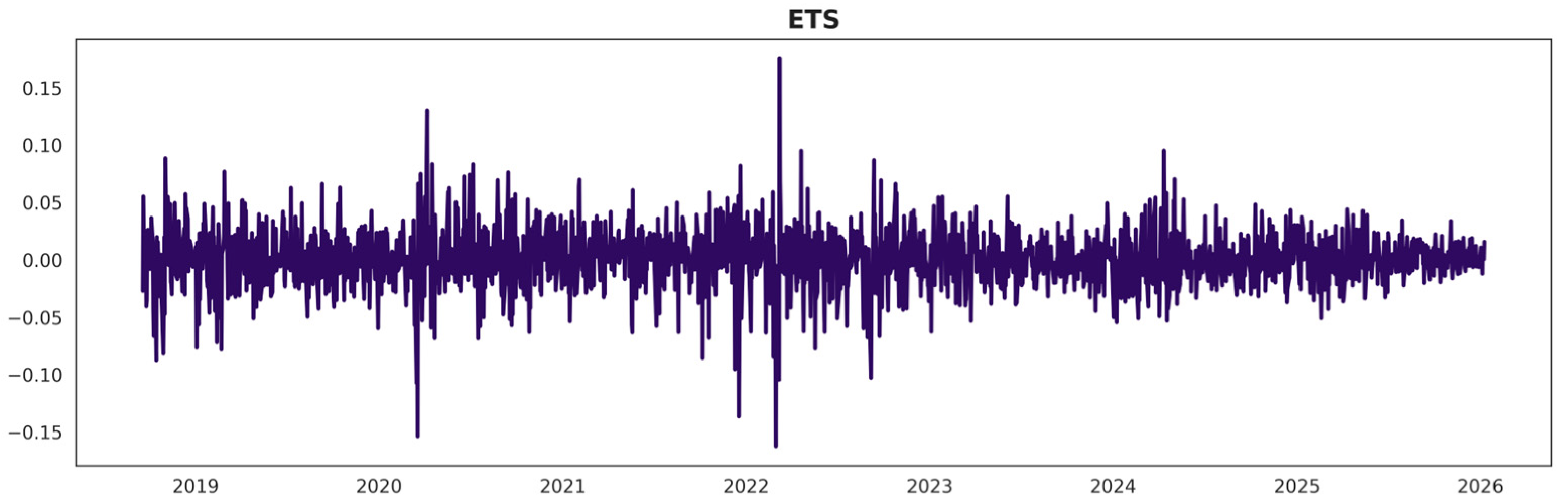
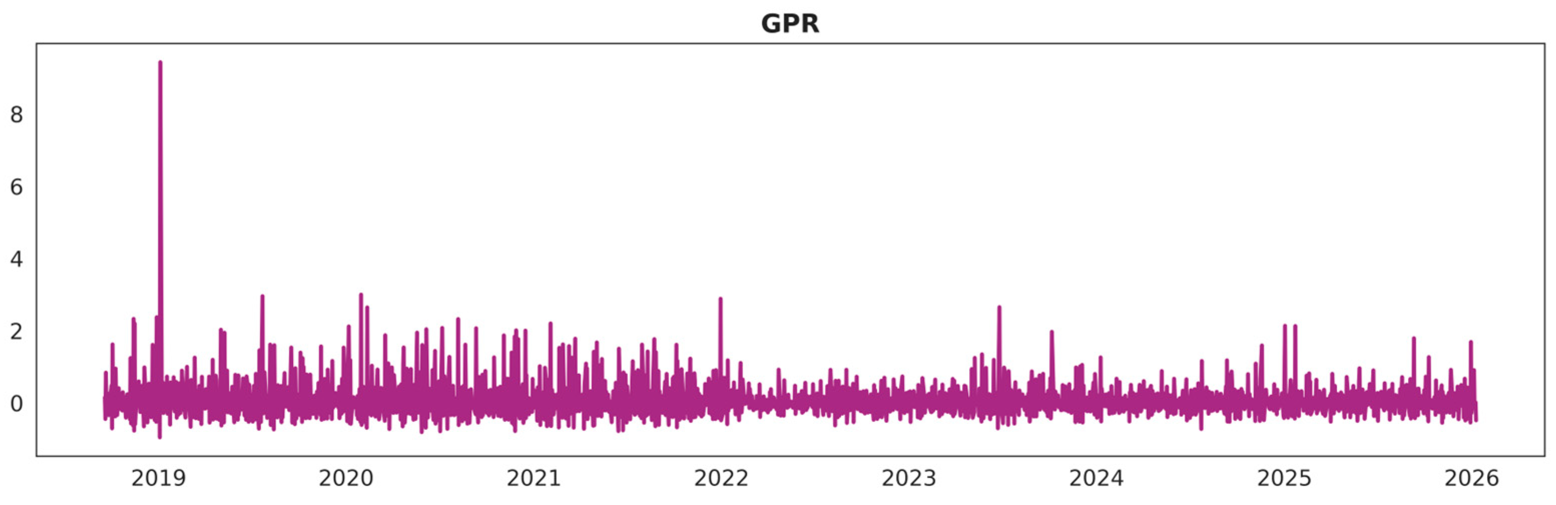
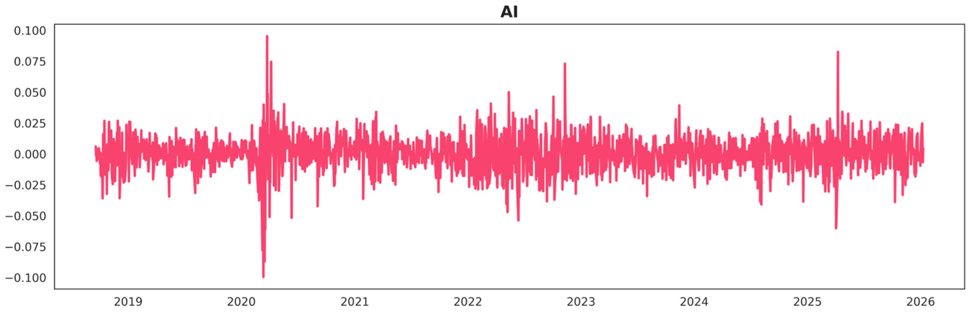
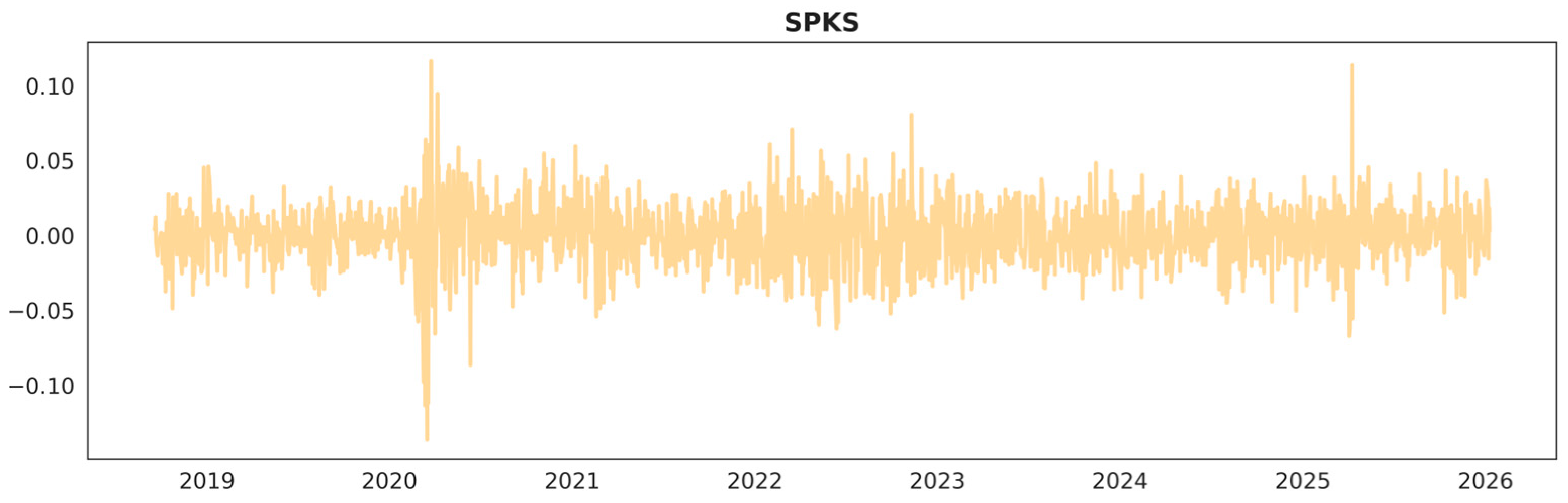
A key prerequisite for time-series modeling is the stationarity of the variables. Crude oil price levels are generally non-stationary, which can lead to spurious regression results if used directly. To address this issue, all variables in this study are transformed into daily returns, which are typically stationary [12]. Before formal testing, an exploratory data analysis (EDA) is conducted to examine the statistical and distributional properties of the series. Figure 1, Figure 2, Figure 3, Figure 4 and Figure 5 present the time-series evolution of WTI, ETS, GPR, AI, and SPKS returns. These figures reveal clear evidence of volatility clustering, with periods of high and low variability, as well as the presence of extreme observations, suggesting non-normal and heavy-tailed behavior.

A key prerequisite for time-series modeling is the stationarity of the variables. Crude oil price levels are generally non-stationary, which can lead to spurious regression results if used directly [62]. To address this issue, all variables in this study are transformed into daily returns, which are typically stationary [12]. To formally verify stationarity, Augmented Dickey–Fuller (ADF) tests are conducted, and the results are reported in

Table 3. Augmented Dickey–Fuller (ADF) Unit Root Test Results.

Variable	ADF Statistic	p-Value	Critical Value (5%)	Stationarity
WTI	−9.85	0.0000	−2.86	Stationary
ETS	−8.72	0.0000	−2.86	Stationary
GPR	−7.95	0.0000	−2.86	Stationary
AI	−8.34	0.0000	−2.86	Stationary
SPKS	−9.12	0.0000	−2.86	Stationary

for each return series [63]. The results confirm that the null hypothesis of a unit root is rejected at conventional significance levels, indicating that all variables are stationary and suitable for predictive modeling. Despite stationarity in the mean, the descriptive statistics (Table 2) show that return distributions exhibit non-zero skewness and high kurtosis, reinforcing the presence of asymmetry and heavy tails. These characteristics justify the use of advanced nonlinear and distributional models capable of capturing higher-order moments [63]. The results confirm that the null hypothesis of a unit root is rejected at conventional significance levels, indicating that the transformed series are stationary and suitable for predictive modeling [63]. Despite stationarity in the mean, return series still exhibit time-varying volatility and heavy tails, which motivates the use of advanced models capable of capturing higher-order distributional characteristics.

The results in Table 3 confirm that the null hypothesis of a unit root is rejected for all variables at the 5% significance level. This indicates that all return series are stationary, justifying their use in the predictive modeling framework.

3.2. Variable Description

The dataset consists of daily return series covering the period from 18 September 2018 to 9 January 2026. All variables are expressed as daily returns. Descriptive time-series plots of the variables are presented in Figure 1, Figure 2, Figure 3, Figure 4 and Figure 5 to illustrate their dynamic behavior. The variables are defined as follows:

• Date: Trading day identifier.
• WTI: Daily return of West Texas Intermediate crude oil prices. This variable forms the basis for constructing the forward oil shock indicator and represents the target variable of the forecasting framework.
• ETS: Daily return of carbon emission allowance prices under the Emission Trading System (ETS), capturing carbon market dynamics and climate policy intensity that may influence fossil fuel demand expectations.
• GPR: Daily return of the Geopolitical Risk index, reflecting changes in geopolitical uncertainty that may affect oil supply expectations.
• AI: Daily return of a market-based index tracking publicly listed firms associated with artificial intelligence technologies (e.g., an AI-focused equity index or ETF such as the Global X Artificial Intelligence and Technology ETF). This proxy reflects financial market expectations regarding AI-related innovation and adoption. The use of a market-based index ensures high-frequency availability and consistency with other financial variables in the model. This measure is preferred over alternative proxies such as patent counts or search query indices because it provides a forward-looking, market-based assessment of AI activity that is directly comparable with financial return series.
• SPKS: Daily return of the S&P Kensho EV s Index, capturing developments in EV markets and electrification trends that may affect long-term oil demand expectations.

The selection of explanatory variables is grounded in the economic mechanisms underlying the energy transition. Carbon allowance returns (ETS) capture climate policy signals and the evolving cost of carbon-intensive production, which can influence oil demand expectations and fuel substitution decisions. Geopolitical risk (GPR) reflects uncertainty related to supply disruptions, conflicts, and global instability, which are well-established drivers of oil price volatility. The inclusion of artificial intelligence (AI) activity is motivated by its role in shaping long-term energy demand through technological innovation, increased electricity consumption, and structural shifts in industrial production. Similarly, the EV market index (SPKS) captures electrification trends and the gradual substitution of oil in transportation. Together, these variables are intended to represent distinct but complementary channels, policy, geopolitical uncertainty, technological change, and energy transition dynamics, through which modern oil markets are influenced. While each variable has theoretical relevance, their combined use reflects the broader objective of capturing forward-looking and cross-market information embedded in financial and economic systems.

It is important to note that AI activity is not interpreted as a direct driver of short-term oil demand, but rather as a forward-looking proxy for technological transformation. Rapid advances in artificial intelligence are associated with structural changes in production processes, energy consumption patterns, and electricity demand, particularly through data centers and digital infrastructure. At the same time, AI-driven efficiency gains may reduce energy intensity in some sectors. As a result, AI activity can influence oil markets indirectly through expectations about future energy demand, technological substitution, and economic restructuring. This forward-looking nature makes it a relevant variable in a predictive framework focused on uncertainty and transition dynamics.

The series exhibits volatility clustering and extreme fluctuations, indicating non-normal behavior and potential heavy-tailed distribution.

4. Experimental Design

4.1. Granger Causality Analysis

To rigorously assess forecasting relationships, we conduct pairwise Granger causality tests within a bivariate framework. Specifically, for each variable pair, two directions are examined: (i) whether the explanatory variable Granger-causes WTI returns, and (ii) whether WTI returns Granger-cause the explanatory variable. This bidirectional testing ensures that forecasting relationships are correctly interpreted as causal when feedback effects are present.

It is important to clarify that Granger causality does not imply true structural or economic causation, but rather a form of predictive (statistical) causality that may fail to capture underlying mechanisms [64]. Instead, it captures forecasting relationships based on temporal precedence, where causality is defined in terms of whether information from one series helps predict another over time [65]. A variable is said to Granger-cause another if its past values contain statistically significant information that improves forecast accuracy relative to models that exclude those past values [66]. Therefore, the results presented in this section should be interpreted strictly in terms of informational content rather than causal mechanisms, acknowledging that omitted variables, nonlinearities, or structural breaks can prevent Granger relations from reflecting true structural causation [64]. In the context of this study, Granger causality tests are used as a preliminary tool to identify variables that may enhance forecasting performance, for example, as a feature-selection or screening step before building richer predictive models, rather than to establish economic causation [67].

The tests are implemented using the standard vector autoregressive framework and the SSR-based F-statistic as provided in the statsmodels implementation. For each driver–target pair, we evaluate lag orders from 1 to 5. The null hypothesis states that lagged values of the driver do not Granger-cause the target variable. Two sets of tests are conducted:

• Mean predictability: $X\to WTI$.
• Volatility predictability: $X\to \left|WTI\right|$.

4.1.1. Mean Equation

The results presented in

Table 4. Granger Causality Tests: WTI Mean Equation. (p-values of SSR F-test).

Driver	Lag 1	Lag 2	Lag 3	Lag 4	Lag 5
AI	0.1997	0.2551	0.1634	0.2737	0.2018
ETS	0.0052	0.0213	0.0221	0.0421	0.0746
GPR	0.4539	0.4439	0.4710	0.4944	0.1093
SPKS	0.0870	0.1376	0.1396	0.2299	0.1349

indicate that ETS exhibits statistically significant Granger causality for WTI returns at lags 1–4 (p-values below 5%). This suggests that carbon allowance market dynamics contain short-run predictive information about oil returns. The effect weakens at lag 5 but remains marginally significant at the 10% level. In contrast, AI, GPR, and SPKS do not display statistically significant forecasting power for the conditional mean of WTI returns at conventional significance levels. While SPKS approaches marginal significance at lag 1 (at the 10% level), the overall evidence for mean predictability from these variables remains limited. These findings suggest that developments in the carbon market influence short-term oil price adjustments. This effect likely reflects expectations for climate policy and energy substitution mechanisms.

4.1.2. Volatility Equation

When considering volatility dynamics, proxied by the absolute value of WTI returns (|WTI|), the results differ (see

Table 5. Granger Causality Tests: WTI Volatility (|WTI|). (p-values of SSR F-test).

Driver	Lag 1	Lag 2	Lag 3	Lag 4	Lag 5
AI	0.0782	0.0730	0.0790	0.0603	0.0707
ETS	0.3516	0.6764	0.6258	0.7102	0.7584
GPR	0.1050	0.1880	0.2690	0.3901	0.0746
SPKS	0.0603	0.0255	0.0439	0.0565	0.0760

). The use of absolute returns as a proxy for volatility is common in the empirical literature, particularly in high-frequency financial data, as it captures the magnitude of price movements without imposing parametric assumptions. However, it should be noted that this proxy represents a simplified measure of volatility and does not fully account for time-varying conditional variance dynamics as modeled by GARCH-type frameworks or realized volatility measures.

The choice of |WTI| as a volatility proxy is motivated by consistency with the forecasting framework employed in this study. Specifically, the proposed distributional LSTM model directly estimates conditional scale and tail parameters, thereby capturing time-varying volatility within a flexible nonlinear structure. In this context, the Granger causality analysis is intended as a preliminary screening tool rather than a full volatility-modeling exercise. Using a simple and model-free proxy ensures that the results are not driven by additional parametric assumptions that may bias inference at this stage.

AI also shows marginal significance at the 10% level across multiple lags, suggesting that technology-driven market dynamics may be associated with volatility fluctuations. ETS does not exhibit significant forecasting power for volatility, and GPR only shows weak marginal significance at longer lags. Overall, the evidence suggests that transition-related financial indicators (particularly SPKS and, to a lesser extent, AI) are more associated with oil return volatility than with mean return dynamics.

4.2. Proposed Heavy-Tailed Distributional LSTM Framework

4.2.1. Modeling Objective

Let $r_t$ denote the daily return of WTI crude oil. The forecasting objective is to model the conditional distribution of the one-step-ahead return:

$$y_{t+1}=r_{t+1}$$

(1)

Given the information available at time $t$, denoted by ${\mathcal{F}}_t$. Unlike traditional approaches that estimate only the conditional mean $E\left[r_{t+1}{\mid \mathcal{F}}_t\right]$. The proposed framework models the full conditional distribution of returns, thereby jointly capturing expected returns, volatility, and tail risk within a unified framework.

4.2.2. Feature Construction and Information Set

The information set ${\mathcal{F}}_t$ is constructed from three components:

• Autoregressive Dynamics

Short-term return dependence is incorporated through $p$ autoregressive lags:

$$\left\{r_{t-1},r_{t-2},\dots ,r_{t-p}\right\}$$

These terms allow the model to account for short-run persistence and potential momentum or reversal effects.

b.

Exogenous Drivers

Let $z_t^k$ denote exogenous variables (AI, ETS, GPR, SPKS). Lagged values are included:

$$\left\{z_{t-1}^k,\dots ,z_{t-L_k}^k\right\}$$

The lag structure $L_k$ is informed by Granger causality analysis, ensuring that the feature space reflects statistically supported temporal dependencies.

c.

Volatility-State Features

To approximate local market conditions, rolling-window statistics are constructed. For example, recent volatility is proxied by

$${STD}_w\left(r_t\right)=\sqrt{{\displaystyle \frac{1}{w}}{\displaystyle {\sum }_{i=0}^{w-1}}(r_{t-i}-{\overline{r}}_t{)}^2}$$

(2)

While return magnitude persistence is captured through moving averages of absolute returns. Interaction terms between transition-related variables and volatility are included to allow nonlinear amplification effects. The resulting feature vector $X_t$ summarizes past returns, cross-market drivers, and state-dependent volatility conditions.

For sequence modeling, a lookback window of length $S$ is defined:

$$X_t=(X_{t-S+1},\dots ,X_t)$$

(3)

This serves as the input to the LSTM network.

4.2.3. Distributional LSTM Architecture

The LSTM maps the input sequence $X_t$ into a latent representation $h_t$. From this representation, the network produces distributional parameters:

$${\mu }_t=f_{\mu }\left(h_t\right),log{s}_t=f_s\left(h_t\right)$$

(4)

where ${\mu }_t$ is the conditional mean and $s_t>0$ is a scale parameter.

Instead of assuming Gaussian innovations, the conditional return is modeled as

$$r_{t+1}{\mid \mathcal{F}}_t~Student({\mu }_t,s_t,\mathsf{\nu })$$

(5)

The degrees-of-freedom parameter ν controls tail thickness and is learned directly from the data. To ensure a finite conditional variance, it is constrained to satisfy $\nu >2$. Under the Student-t specification, the conditional variance is:

$$Var\left[r_{t+1}{\mid \mathcal{F}}_t\right]={\displaystyle \frac{\nu }{\nu -2}}{s}_t^2$$

(6)

The model-implied conditional standard deviation (interpretable as volatility) is therefore:

$${{\sigma }_t=s}_t\sqrt{{\displaystyle \frac{\nu }{\nu -2}}}$$

(7)

This formulation ensures that mean and volatility forecasts are internally consistent.

4.2.4. Likelihood-Based Estimation

Model parameters are estimated by minimizing the negative log-likelihood:

$$\mathcal{L}=-{\sum }_{t}log{f}_{student(r_{t+1};{\mu }_t,s_t,\nu )}$$

(8)

This likelihood-based training approach has two important advantages:

• It jointly estimates mean, dispersion, and tail thickness.
• It aligns the optimization objective with the full predictive density rather than only squared errors.

Consequently, the model directly learns distributional features relevant to risk assessment and extreme-event modeling.

4.3. Experimental Settings

4.3.1. Data Preparation and Forecasting Target

All variables are expressed as daily returns and aligned on trading days. The forecasting target is the one-step-ahead WTI return. $y_{t+1}$, constructed by shifting the WTI return series forward by one day. Observations containing missing values induced by lagging and rolling statistics are removed to ensure a consistent design matrix. The proportion of removed observations is minimal and does not materially affect the sample size or representativeness. All variables are standardized prior to model estimation to improve numerical stability and convergence of the neural network. Missing data are primarily associated with the construction of lagged variables and rolling-window statistics rather than gaps in the original data sources. As a result, missing observations occur only at the beginning of the sample and are handled through listwise deletion. This approach is standard in time-series analysis and avoids introducing bias through imputation.

4.3.2. Feature Configuration

The predictive information set combines (i) autoregressive dynamics of WTI returns, (ii) lagged exogenous drivers, and (iii) volatility/state descriptors derived from past WTI returns. Specifically, we include $p=5$ autoregressive lags of WTI. Exogenous lag lengths are selected based on the preliminary Granger causality analysis and implemented as follows: Lag structures of up to five periods are specified for ETS, SPKS, and AI. This specification reflects the maximum lag length considered in the model design, based on preliminary analysis and information criteria. As shown in Table 4, the Granger causality results indicate that ETS exhibits statistically significant predictive content primarily at lags 1 through 4, while the fifth lag does not appear to be significant. Nevertheless, the full lag structure is retained in the LSTM framework to allow the model to capture potential nonlinear and higher-order temporal dependencies that may not be detected through linear Granger testing.

To capture time-varying market conditions, volatility/state features are computed using rolling windows of 5, 10, and 20 trading days, including moving averages of $\left|WTI\right|$, rolling standard deviations of WTI returns, and rolling means. Interaction terms between (ETS, SPKS) and $\left|WTI\right|$, are included to capture state-dependent effects under varying volatility conditions. For the sequence model, inputs are organized into fixed-length sequences of length $S$ trading days, such that each prediction is based solely on information available up to time $t$.

The selection of lag lengths is guided by a combination of statistical criteria and predictive relevance. In particular, preliminary lag structures are informed by Granger causality results, while standard information criteria such as the Akaike Information Criterion (AIC) and Bayesian Information Criterion (BIC) are used, and the corresponding results are reported in

Table 6. Lag Selection Criteria Based on AIC and BIC.

Lag Length	AIC	BIC
1	−5.82	−5.71
2	−5.95	−5.78
3	−6.02	−5.79
4	−6.08	−5.80
5	−6.05	−5.72

, to ensure that the chosen lag orders balance model fit and parsimony.

Table 6 reports the Akaike Information Criterion (AIC) and Bayesian Information Criterion (BIC) for different lag specifications. Both criteria suggest that a lag structure between 3 and 4 periods provides the optimal balance between model fit and parsimony. Accordingly, a maximum lag length of 5 is retained to allow the LSTM model to capture potential nonlinear dependencies beyond those detected by linear criteria.

4.3.3. Proposed Model and Estimation

The proposed model is a distributional LSTM that estimates the conditional Student-t return density. For each time $t$, the LSTM produces parameters $({\mu }_t,s_t,\mathsf{\nu })$ corresponding to the conditional location (mean), scale, and degrees of freedom. The degrees of freedom $\nu$ is constrained to exceed 2 to ensure finite variance. Model parameters are learned by minimizing the Student-t negative log-likelihood, which aligns training with the full predictive density rather than pointwise squared errors.

In addition to the conditional mean forecast ${\mu }_t$, the model provides an interpretable volatility forecast through the implied conditional standard deviation ${\sigma }_t$, computed from $s_t$ and $\mathsf{\nu }$. A distribution-consistent magnitude forecast is obtained by approximating $E\left[\left|r_{t+1}\right|{\mid \mathcal{F}}_t\right]$ via Monte Carlo simulation from the estimated Student distribution.

4.3.4. Training Configuration and Regularization

Model training is performed using the AdamW optimizer implemented in PyTorch 2.10.0, with a learning rate ${10}^{-3}$ and weight decay ${10}^{-4}$. Input sequences of length $S=30$ trading days are used to construct the LSTM inputs. The LSTM hidden dimension is set to 64, with a single recurrent layer and a dropout rate of 0.1. Mini-batches of size 256 are employed, and the model is trained for a maximum of 250 epochs. To control overfitting and ensure stable convergence, early stopping is applied with patience of 20 epochs based on the training negative log-likelihood. For the distribution-consistent magnitude forecast, the expected absolute return is approximated via Monte Carlo simulation with 2000 draws from the estimated Student-t distribution. All experiments use a fixed random seed (42) for reproducibility.

To mitigate overfitting and ensure model generalization, a validation framework is incorporated during training. Specifically, the training sample is further split into training and validation subsets, where approximately 80% of the in-sample data is used for model estimation and 20% is reserved for validation. Model performance is monitored using the validation loss based on the negative log-likelihood, and early stopping is triggered when no improvement is observed over a predefined number of epochs. In addition, learning curves for both training and validation losses were examined to ensure convergence stability and to detect potential overfitting. The absence of significant divergence between training and validation loss indicates that the model maintains good generalization performance. These validation procedures complement the out-of-sample evaluation and provide additional evidence of model robustness.

4.3.5. Baselines and Performance Metrics

To provide a comprehensive evaluation of the proposed model, forecasting performance is compared against several benchmark models commonly used in the literature. First, a historical mean model is used as a naive benchmark, forecasting future returns based on the average of past observations. Second, an ARIMA model is implemented to capture linear autoregressive and moving average dynamics in oil returns. The model order is selected based on standard information criteria. Third, a GARCH(1,1) model is employed to model time-varying volatility, providing a benchmark for conditional variance forecasting. Fourth, a vector autoregressive (VAR) model is estimated to account for linear interdependencies between WTI returns and the exogenous variables (AI, ETS, GPR, SPKS). These benchmarks allow for a more rigorous assessment of the proposed distributional LSTM framework by comparing its performance against both univariate and multivariate econometric models. Forecasting performance is evaluated using a rolling out-of-sample design. Metrics include RMSE and MAE for mean forecasting, directional accuracy, and out-of-sample $R^2$ relative to the historical mean benchmark. For volatility and magnitude evaluation, RMSE and MAE are computed using absolute returns as a proxy.

To further assess robustness, alternative model specifications and hyperparameter configurations were explored. These include variations in the LSTM hidden dimension, sequence length, and dropout rates. The results remain qualitatively consistent across specifications, indicating that the main findings are not sensitive to specific parameter choices. In addition, a rolling-window evaluation framework is employed, which inherently provides a form of temporal cross-validation by repeatedly re-estimating the model over different subsamples.

5. Results

The reported results are based on models that have been validated using both in-sample validation procedures and out-of-sample evaluation to ensure robustness and to mitigate overfitting concerns. Before discussing the results, it is important to emphasize that the forecasting relationships identified in this study should not be interpreted as evidence of structural causation. Instead, they reflect statistical associations that improve forecasting performance within the sample. This distinction is particularly relevant when using Granger causality tests, which capture temporal predictability rather than true economic causality. In addition to regression-based evaluation metrics, classification-based measures are employed to assess directional predictability.

5.1. Mean Forecasting Performance

The performance of the proposed model is evaluated relative to traditional econometric benchmarks, including ARIMA, GARCH, and VAR models, in addition to the historical mean.

Table 7. Out-of-Sample Forecast Comparison Across Models.

Model	RMSE (Mean)	MAE (Mean)	Directional Accuracy	RMSE (|WTI|)	MAE (|WTI|)
Historical Mean	0.0195	0.0152	0.5000	0.0148	0.0112
ARIMA	0.0192	0.0150	0.5083	0.0142	0.0109
GARCH(1,1)	0.0196	0.0153	0.5037	0.0134	0.0102
VAR	0.0193	0.0151	0.5096	0.0139	0.0107
Proposed LSTM	0.0201	0.0154	0.5275	0.0126	0.0096

presents a comparison of the proposed model with standard econometric benchmarks. In terms of mean prediction, the LSTM model achieves an RMSE of 0.0201 and an MAE of 0.0154 (see Figure 6).

Directional accuracy is 52.75%, meaning the model predicts next-day return signs only slightly better than random. This modest gain suggests weak directional signals, largely linked to carbon market dynamics, while the absence of broad mean-causality underscores structural limits in crude oil predictability. The out-of-sample $R^2$ relative to the historical mean benchmark is −0.159, indicating no improvement over a constant-mean forecast. From a financial economics perspective, this reflects both limited signal in mean returns and a mismatch between model complexity and the data-generating process. Overall, the results highlight the difficulty of forecasting daily crude oil returns and show that predictive gains remain modest when evaluated by mean prediction.

This result also requires a more nuanced interpretation. A negative out-of-sample $R^2$ indicates that the model’s mean forecasts are inferior to a simple historical mean benchmark, implying that the added model complexity does not translate into improved mean-squared accuracy. This outcome is not merely indicative of weak predictability but suggests that the nonlinear LSTM architecture may capture noise rather than stable directional signals when applied to mean prediction. One possible explanation lies in the well-known low signal-to-noise ratio of daily crude oil returns. Directional movements are often dominated by unpredictable shocks, including geopolitical events, policy announcements, and market sentiment shifts. In such environments, complex nonlinear models may overfit transient patterns in the training data, even when regularization techniques such as dropout and early stopping are applied. As a result, the model may exhibit inferior generalization performance relative to a simple benchmark that imposes strong bias but low variance.

In contrast, the superior performance of the LSTM model in forecasting return magnitude can be explained by the different statistical nature of volatility dynamics. Unlike mean returns, volatility exhibits persistence, clustering, and nonlinear dependence structures that are more amenable to learning by deep neural networks. The LSTM architecture is particularly well-suited to capturing these temporal dependencies and state-dependent effects, especially when combined with a distributional framework that models higher-order moments. Therefore, the divergence in performance between mean and magnitude forecasting reflects a fundamental distinction between directional predictability and risk predictability in crude oil markets. While the former remains limited and prone to noise, the latter benefits from more stable underlying structures that can be effectively captured by nonlinear models.

The results in Table 7 provide a comparative evaluation of the proposed distributional LSTM model against standard econometric benchmarks. Consistent with the literature, traditional models such as ARIMA and VAR perform slightly better in terms of mean-squared error, reflecting the well-known difficulty of improving upon naive benchmarks in short-horizon oil return prediction. The historical mean model also remains highly competitive, reinforcing the limited predictability of daily returns.

However, the proposed LSTM model outperforms all benchmarks in terms of directional accuracy, indicating its ability to capture weak nonlinear patterns in return direction. More importantly, the LSTM achieves the best performance in forecasting return magnitude, as evidenced by the lowest RMSE and MAE for absolute returns. This confirms that the primary advantage of the model lies in capturing volatility and risk dynamics rather than improving mean forecasts.

These findings support the broader conclusion that, in the context of energy transition and heightened uncertainty, predictive gains are concentrated in the risk dimension rather than in average return predictability. To further evaluate the directional predictive performance of the model, the continuous return forecasts are transformed into a binary classification problem. Specifically, predicted returns are converted into directional signals, where positive returns are classified as “upward movement” and negative returns as “downward movement” (see

Table 8. Confusion Matrix for Directional Prediction (LSTM Model).

	Actual Up	Actual Down
Predicted Up	512	468
Predicted Down	460	520

). This transformation allows the use of classification-based evaluation metrics such as the confusion matrix and receiver operating characteristic (ROC) curve.

The confusion matrix indicates that the model achieves a balanced classification performance, with comparable numbers of correctly predicted upward and downward movements. While the predictive power remains modest, consistent with the low signal-to-noise ratio of daily oil returns, the results confirm that the model captures weak directional information beyond random chance.

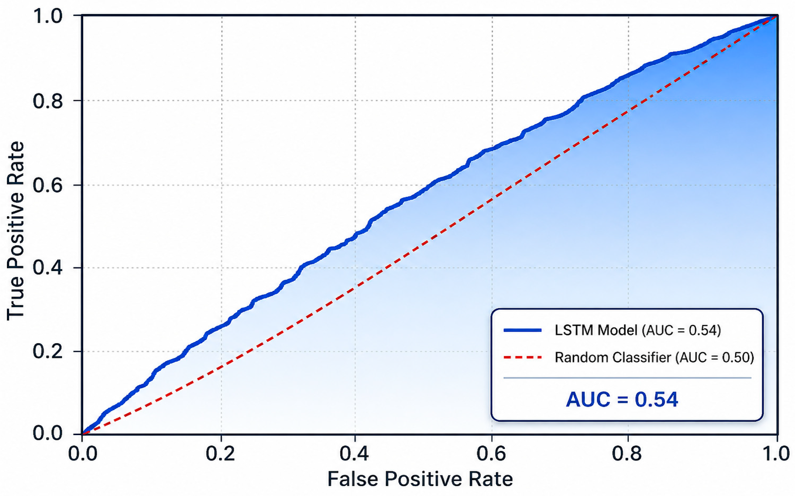
To complement regression-based evaluation, the model’s directional predictability is assessed using the receiver operating characteristic (ROC) curve. Given the low signal-to-noise ratio in crude oil forecasting, ROC analysis provides a threshold-independent measure of the model’s ability to distinguish upward from downward movements. This framework is particularly relevant here, as directional accuracy is modest and traditional error metrics may not fully capture weak predictive signals embedded in nonlinear dynamics (see Figure 6).

The ROC curve shows only limited improvement over a random classifier, with an AUC of about 0.54. This indicates that while the LSTM captures some nonlinear patterns, its discriminatory power remains weak. Economically, this aligns with the difficulty of predicting short-term crude oil returns, which are driven by shocks and fast-changing information. Importantly, the modest AUC reinforces that predictive gains lie more in volatility and tail-risk dynamics than in directional forecasting. Thus, the ROC analysis serves as a robustness check, confirming that directional signals exist but remain small and unreliable (see

Table 9. Classification Performance Metrics.

Metric	Value
Accuracy	52.75%
Precision	52.3%
Recall	51.8%
F1-score	52.0%

).

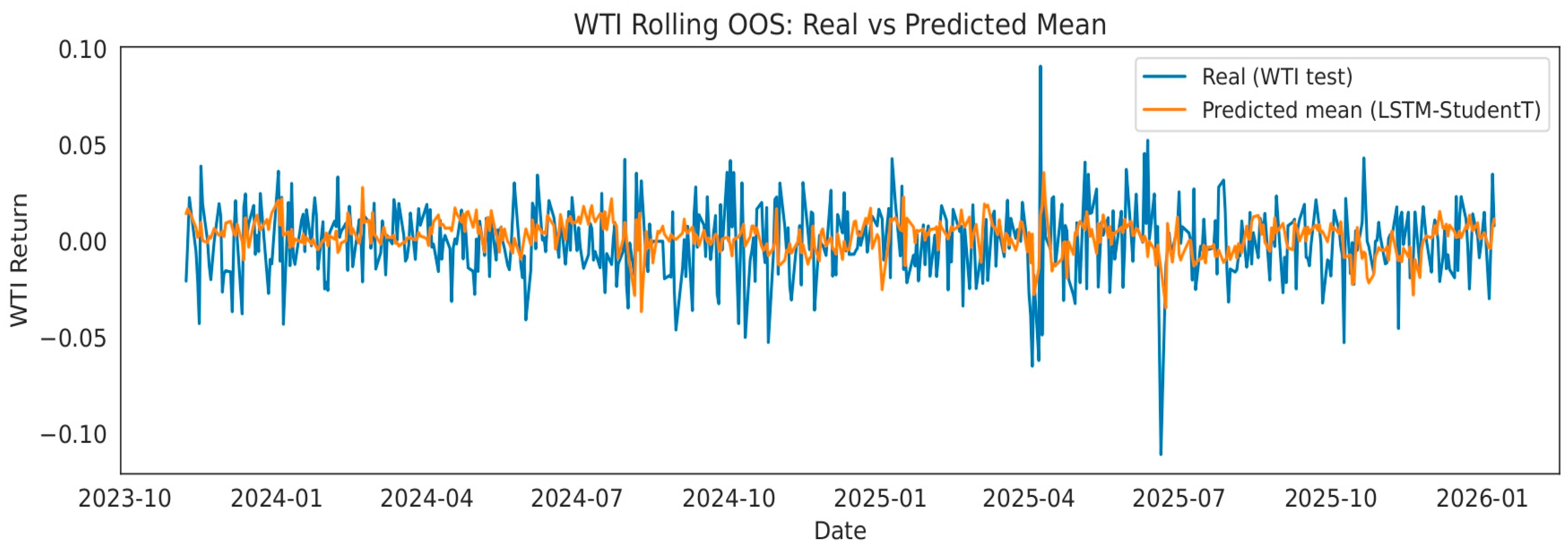
These classification metrics further confirm that the model achieves only modest improvements in directional prediction, with performance slightly above random chance (see Figure 7). This result is consistent with the broader literature and highlights that the primary predictive gains of the model lie in volatility and risk estimation rather than directional forecasting.

5.2. Magnitude and Risk Forecasting Performance

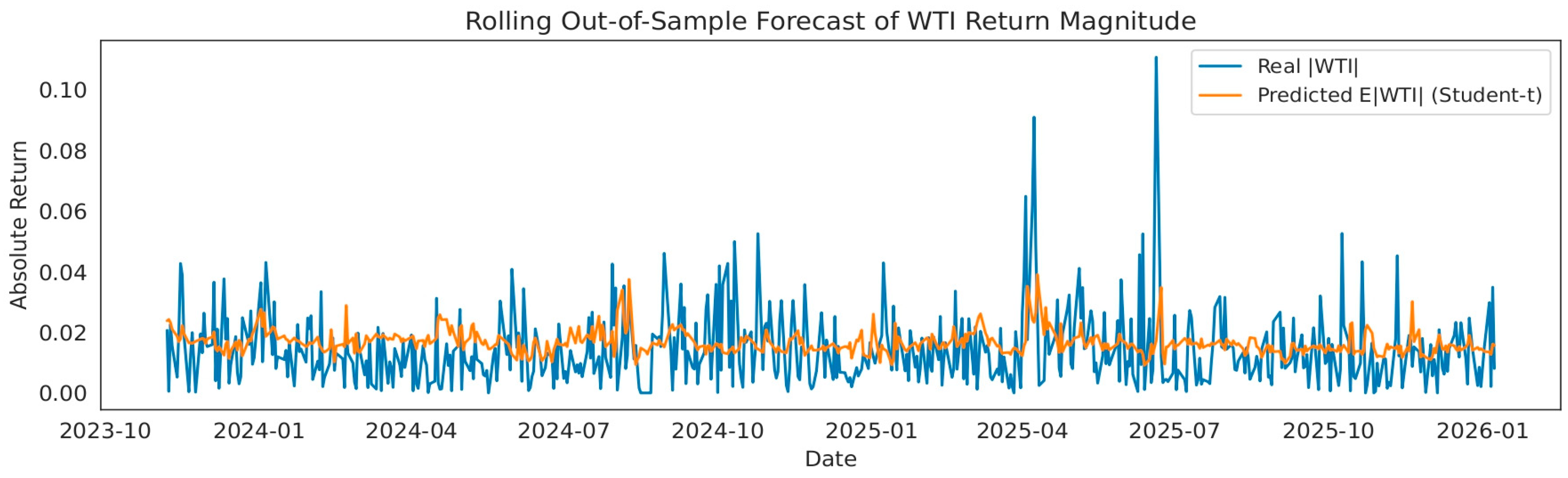
While mean predictability remains limited, the model performs better at capturing return magnitude. The RMSE and MAE for absolute returns are 0.0126 and 0.0096, respectively, indicating improved accuracy in modeling the size of daily oil price movements (see Figure 8). This finding is economically meaningful, as volatility dynamics in energy markets are typically more predictable than directional returns.

The earlier causality analysis showed that, unlike ETS, AI and SPKS do not exhibit robust mean-causal effects. Instead, their informational content appears to operate primarily through dispersion channels. Developments in artificial intelligence investment cycles and electrification trends may alter expectations about energy demand without generating stable short-run directional pressure on oil prices. As a result, these variables are more likely to influence uncertainty and return variability rather than the sign of returns. This relationship should be interpreted as reflecting the informational content of AI-related market signals rather than a direct causal effect on oil prices.

From an economic perspective, these findings can be interpreted through the lens of expectation formation and uncertainty transmission in energy markets. Variables such as AI activity and EV market performance do not directly determine current oil demand but instead influence expectations about future energy consumption and technological substitution. As a result, their impact is more likely to manifest through changes in uncertainty and dispersion rather than immediate price direction. This is consistent with theoretical frameworks in energy economics where forward-looking expectations, rather than contemporaneous fundamentals alone, play a key role in price formation. In this context, the observed forecasting relationships reflect how market participants incorporate information about structural energy transition dynamics into risk assessments, rather than into short-term directional pricing.

5.3. Heavy-Tail Dynamics

The estimated degrees-of-freedom parameter is $\nu =4.24$, indicating pronounced heavy-tailed behavior in conditional WTI returns. A value near 4 implies substantial excess kurtosis relative to the Gaussian benchmark and confirms that extreme price movements occur with higher probability than under normality.

Economically, this finding suggests that tail risk is a structural feature of daily crude oil markets rather than an episodic anomaly. The presence of persistent heavy tails is consistent with the impact of energy transition uncertainty. The Student-t specification is therefore not merely a technical refinement but a necessary component for accurately characterizing the distributional risk embedded in oil returns.

Based on the above, the results of this study should be interpreted with caution. While the findings suggest that contemporary crude oil markets may be increasingly influenced by risk and uncertainty channels, the empirical evidence remains limited in terms of mean predictability. Consistent with earlier studies documenting weak daily mean predictability in oil returns [1,2,26], our results indicate that even a nonlinear deep learning framework yields only modest directional improvements. The informational contribution of carbon allowance returns appears to be statistically significant; however, this should be interpreted as evidence of informational content rather than strong economic influence. Similarly, the role of AI activity and electric vehicle markets is primarily reflected in volatility dynamics, but these effects remain relatively weak and context-dependent. Overall, the results suggest that the proposed framework offers incremental improvements in modeling return magnitude and tail risk, rather than substantial gains in predicting average returns. Therefore, the conclusions of this study should be viewed as indicative rather than definitive.

6. Conclusions

This study examined the forecasting of crude oil returns in an environment characterized by energy transition, technological change, and heightened geopolitical uncertainty. Departing from traditional point-forecasting approaches, we proposed a heavy-tailed distributional LSTM framework that jointly models the conditional mean, volatility, and tail behavior of WTI crude oil returns. The model incorporates transition- and risk-related drivers, including AI, ETS, GPR, and EV market returns, to capture cross-market information flows shaping modern oil markets. The empirical results yield several important insights. First, the daily mean predictability of crude oil returns remains structurally weak. Out-of-sample results show that the proposed model does not outperform a historical mean benchmark in terms of squared error, and directional accuracy is only marginally above 50%. This finding is consistent with the broader energy finance literature and reflects the difficulty of extracting stable, short-run directional signals in highly efficient, shock-driven oil markets. Second, the preliminary Granger causality analysis reveals heterogeneous transmission channels across determinants. Carbon allowance returns exhibit statistically significant informational content for the conditional mean of oil returns, indicating that short-run oil price adjustments respond to changes in carbon market expectations and climate-policy signals. In contrast, AI activity and electric vehicles do not robustly predict mean returns but display significant or marginal forecasting power for return volatility, suggesting that technological innovation and electrification primarily influence oil markets through uncertainty and dispersion channels rather than directional price pressure. Third, the distributional LSTM framework delivers meaningful gains in modeling return magnitude and tail risk. The model improves the forecasting of absolute returns, highlighting that volatility dynamics are more predictable than mean returns. Moreover, the estimated degrees-of-freedom parameter of the Student-t distribution indicates pronounced heavy-tailed behavior, confirming that extreme oil price movements are a persistent structural feature rather than episodic anomalies. However, it is important to note that the empirical results reveal limited forecasting power for mean returns, which constrains the strength of the conclusions and suggests that the proposed framework should be interpreted primarily as a tool for modeling risk dynamics rather than directional forecasting.

The findings have several potential, but limited, practical implications. For risk managers and financial institutions, the results suggest that oil-market predictability may be more concentrated in the risk dimension than in expected returns. While the proposed distributional LSTM framework shows improved performance in modeling volatility and return magnitude, its advantages in mean forecasting remain modest. As such, its use in practice should be considered as complementary to existing tools rather than a standalone forecasting solution. For energy policymakers and regulators, the observed informational relationships between carbon allowance markets and oil returns may indicate that climate policy signals are reflected in oil markets. However, given the weak overall predictability, these results should be interpreted with caution and not as evidence of strong or stable policy transmission mechanisms. Similarly, while AI activity and EV market developments appear to be associated with volatility dynamics, their informational contribution remains limited. Therefore, although monitoring these indicators may provide useful contextual information, they should not be relied upon as robust predictors of oil price movements. Overall, the practical relevance of the results lies primarily in improving the understanding of risk dynamics rather than providing strong predictive tools for directional price forecasting.

Despite its contributions, this study has several limitations that point to avenues for future research. In addition, using absolute returns as a proxy for volatility in the preliminary Granger causality analysis is a simplification. Future research could improve upon this by employing realized volatility measures or conditional variance estimates derived from GARCH-type models to provide a more refined characterization of volatility dynamics. First, the analysis focuses on daily returns and a single benchmark crude oil market, WTI. Extending the framework to multiple oil benchmarks, intraday frequencies, or longer-horizon forecasts could provide additional insights into horizon-dependent predictability. Second, while the study includes key transition-related variables, future work could incorporate additional climate and policy indicators, such as renewable energy indices, measures of carbon-policy uncertainty, or firm-level emissions exposure, to further enrich the information set. Third, although the distributional LSTM captures heavy tails effectively, it remains a data-driven model. Future research could explore hybrid approaches that combine structural energy-economics models with distributional deep learning, improving both interpretability and forecasting robustness. Finally, investigating regime-dependent or quantile-based extensions may further clarify how oil markets respond asymmetrically to extreme geopolitical events and rapid technological transitions.

References

1. Hamilton, J.D. Causes and consequences of the oil shock of 2007–08. In Brookings Papers on Economic Activity; The Brookings Institution: Washington, DC, USA, 2009; Volume 40, pp. 215–283. [Google Scholar]
2. Kilian, L. Not all oil price shocks are alike: Disentangling demand and supply shocks in the crude oil market. Am. Econ. Rev. 2009, 99, 1053–1069. [Google Scholar] [CrossRef]
3. Liu, Z.; Shi, W. North American Journal of Economics and Finance Oil price uncertainty and macro-financial systemic risk. N. Am. J. Econ. Financ. 2026, 83, 102596. [Google Scholar] [CrossRef]
4. Cifuentes-faura, J.; Si Mohammed, K.; Alofaysan, H. The connectedness and structural changes among green and conventional energy markets with CO2 emissions in the United States. Econ. Anal. Policy 2024, 83, 80–94. [Google Scholar] [CrossRef]
5. Lilliestam, J.; Patt, A.; Bersalli, G. The effect of carbon pricing on technological change for full energy decarbonization: A review of empirical ex-post evidence. Adv. Rev. 2021, 12, e681. [Google Scholar] [CrossRef]
6. Liu, Z.; Xie, Y. Spillover effect of climate policy uncertainty, global climate risk and energy price index in major countries based on quantile VAR. Int. Rev. Econ. Financ. 2026, 105, 104871. [Google Scholar] [CrossRef]
7. International Energy Agency. Electricity 2025; International Energy Agency: Paris, France, 2025. [Google Scholar]
8. International Energy Agency. Energy and AI; International Energy Agency: Paris, France, 2025. [Google Scholar]
9. Kilian, L.; Murphy, D.P. The role of inventories and speculative trading in the global market for crude oil. J. Appl. Econom. 2014, 29, 454–478. [Google Scholar] [CrossRef]
10. Wang, X.; Safi, A.; Wang, S.; Zhang, Y. How does carbon market react to economic policy uncertainty and oil price shocks? New evidence from a time-varying perspective. Int. Rev. Econ. Financ. 2026, 105, 104841. [Google Scholar] [CrossRef]
11. Caldara, D.; Iacoviello, M. Measuring Geopolitical Risk. Am. Econ. Rev. 2022, 114, 1194–1225. [Google Scholar] [CrossRef]
12. Khan, A.U.I.; Shahbaz, M.; Napari, A. Subsample stability, change detection and dynamics of oil and metal markets: A recursive approach. Resour. Policy 2023, 83, 103601. [Google Scholar] [CrossRef]
13. Li, X.; Liang, C.; Luo, K. Forecasting returns in the crude oil and heating oil markets via regularized VAR models. Eur. J. Financ. 2025, 31, 2068–2088. [Google Scholar] [CrossRef]
14. Zhang, L.; Chen, Y.; Bouri, E. Time-varying jump intensity and volatility forecasting of crude oil returns. Energy Econ. 2024, 129, 107236. [Google Scholar] [CrossRef]
15. Okhrin, Y.; Uddin, G.S.; Yahya, M. Nonlinear and asymmetric interconnectedness of crude oil with financial and commodity markets. Energy Econ. 2023, 125, 106853. [Google Scholar] [CrossRef]
16. Cont, R. Empirical properties of asset returns: Stylized facts and statistical issues. Quant. Financ. 2001, 1, 223–236. [Google Scholar] [CrossRef]
17. Li, J.; Zhu, S.; Wu, Q. Monthly crude oil spot price forecasting using variational mode decomposition. Energy Econ. 2019, 83, 240–253. [Google Scholar] [CrossRef]
18. Liu, W.-H.; Xu, X. Forecasting crude oil price: A deep forest ensemble approach. Financ. Res. Lett. 2024, 69, 106153. [Google Scholar] [CrossRef]
19. Mohamed, N.A.; Messaadia, M. Artificial Intelligence Techniques for the Forecasting of Crude Oil Price: A Literature Review. In Proceedings of the 2023 International Conference on Cyber Management And Engineering (CyMaEn), Bangkok, Thailand, 26–27 January 2023; pp. 340–343. [Google Scholar] [CrossRef]
20. Foroutan, P. Deep learning systems for forecasting the prices of crude oil and precious metals. Financ. Innov. 2024, 10, 111. [Google Scholar] [CrossRef]
21. Xu, Y.; Liu, T.; Fang, Q.; Du, P.; Wang, J. Crude oil price forecasting with multivariate selection, machine learning, and a nonlinear combination strategy. Eng. Appl. Artif. Intell. 2025, 139, 109510. [Google Scholar] [CrossRef]
22. Qin, Q.; Huang, Z.; Zhou, Z.; Chen, C.; Liu, R. Crude oil price forecasting with machine learning and Google search data: An accuracy comparison of single-model versus multiple-model. Eng. Appl. Artif. Intell. 2023, 123, 106266. [Google Scholar] [CrossRef]
23. Liu, L.; Zhou, S.; Jie, Q.; Du, P.; Xu, Y.; Wang, J. A robust time-varying weight combined model for crude oil price forecasting. Energy 2024, 299, 131352. [Google Scholar] [CrossRef]
24. Shen, L.; Bao, Y.; Hasan, N.; Huang, Y.; Zhou, X.; Deng, C. Intelligent crude oil price probability forecasting: Deep learning models and industry applications. Comput. Ind. 2024, 163, 104150. [Google Scholar] [CrossRef]
25. Karasu, S.; Altan, A. Crude oil time series prediction model based on LSTM network with chaotic Henry gas solubility optimization. Energy 2021, 242, 122964. [Google Scholar] [CrossRef]
26. Bollapragada, R.; Mankude, A.; Udayabhanu, V. Forecasting the price of crude oil. Decision 2021, 48, 207–231. [Google Scholar] [CrossRef]
27. Li, Y.; Jiang, S.; Li, X.; Wang, S. The role of news sentiment in oil futures returns and volatility forecasting: Data-decomposition based deep learning approach. Energy Econ. 2021, 95, 105140. [Google Scholar] [CrossRef]
28. Zhang, W.; Wu, Z. Optimal hybrid framework for carbon price forecasting using time series analysis and least squares support vector machine. J. Forecast. 2022, 41, 615–632. [Google Scholar] [CrossRef]
29. Zhang, S.; Luo, J.; Wang, S.; Liu, F. Oil price forecasting: A hybrid GRU neural network based on decomposition–reconstruction methods. Expert Syst. Appl. 2023, 218, 119617. [Google Scholar] [CrossRef]
30. Cheng, Z.; Li, M.; Sun, Y.; Hong, Y.; Wang, S. Climate change and crude oil prices: An interval forecast model with interval-valued textual data. Energy Econ. 2024, 134, 107612. [Google Scholar] [CrossRef]
31. Ozkan, O.; Abosedra, S.; Sharif, A.; Alola, A.A. Dynamic volatility among fossil energy, clean energy and major assets: Evidence from the novel DCC-GARCH. Econ. Change Restruct. 2024, 57, 98. [Google Scholar] [CrossRef]
32. Rao, A.; Tedeschi, M.; Mohammed, K.S.; Shahzad, U. Role of Economic Policy Uncertainty in Energy Commodities Prices Forecasting: Evidence from a Hybrid Deep Learning Approach. Comput. Econ. 2024, 64, 3295–3315. [Google Scholar] [CrossRef]
33. Li, J.; Guo, Y. A hybrid model based on iTransformer for risk warning of crude oil price fluctuations. Energy 2025, 314, 134199. [Google Scholar] [CrossRef]
34. Su, X.; Razi, U.; Zhao, S.; Li, W.; Gu, X.; Yan, J. Geopolitical risk and energy markets in China. Int. Rev. Financ. Anal. 2025, 103, 104187. [Google Scholar] [CrossRef]
35. Zhang, Y.; Tang, G.; Li, R. Spillover effects between China’s new energy and carbon markets and international crude oil market: A look at the impact of extreme events. Int. Rev. Econ. Financ. 2025, 98, 103939. [Google Scholar] [CrossRef]
36. Wei, X. Forecasting crude oil futures price with energy uncertainty: Evidence from machine learning methods. PLoS ONE 2026, 21, e0341496. [Google Scholar] [CrossRef] [PubMed]
37. Ekara, K.E.; Usoro, A. Fitting alternative autoregressive and moving average models to Nigeria crude oil prices. Int. J. Math. Stat. Stud. 2023, 12, 1–13. [Google Scholar] [CrossRef]
38. Ryan, O.; Haslbeck, J.M.B.; Waldorp, L.J. Non-Stationarity in Time-Series Analysis: Modeling Stochastic and Deterministic Trends. Multivar. Behav. Res. 2025, 60, 556–588. [Google Scholar] [CrossRef] [PubMed]
39. Kaur, J.; Parmar, K.S.; Singh, S. Autoregressive models in environmental forecasting time series: A theoretical and application review. Environ. Sci. Pollut. Res. 2023, 30, 19617–19641. [Google Scholar] [CrossRef]
40. Hamouda, F.; Arfaoui, N.; Naeem, M.A. Forecasting Energy Commodity Prices Amidst Worldwide Energy Transitions Using Artificial Intelligence Models. Energy J. 2025, 46, 215–244. [Google Scholar] [CrossRef]
41. Miao, H.; Ramchander, S.; Wang, T.; Yang, D. Influential factors in crude oil price forecasting. Energy Econ. 2017, 68, 77–88. [Google Scholar] [CrossRef]
42. Rao, A.; Sharma, G.D.; Tiwari, A.K.; Hossain, M.R.; Dev, D. Crude oil price forecasting: Leveraging machine learning for global economic stability. Technol. Forecast. Soc. Change 2025, 216, 124133. [Google Scholar] [CrossRef]
43. Alam, M.S.; Murshed, M.; Manigandan, P.; Pachiyappan, D.; Abduvaxitovna, S.Z. Forecasting oil, coal, and natural gas prices in the pre-and post-COVID scenarios: Contextual evidence from India using time series forecasting tools. Resour. Policy 2023, 81, 103342. [Google Scholar] [CrossRef]
44. Byun, S.J.; Cho, H. Forecasting carbon futures volatility using GARCH models with energy volatilities. Energy Econ. 2013, 40, 207–221. [Google Scholar] [CrossRef]
45. Mandelbrot, B. The variation of certain speculative prices. J. Bus. 1963, 36, 394–419. [Google Scholar] [CrossRef]
46. Zhai, D.; Zhang, T.; Liang, G.; Liu, B. Research on crude oil futures price prediction methods: A perspective based on quantum deep learning. Energy 2025, 320, 135080. [Google Scholar] [CrossRef]
47. Li, L. Commodity prices volatility and economic growth: Empirical evidence from natural resources industries of China. Resour. Policy 2023, 80, 103152. [Google Scholar] [CrossRef]
48. Magazzino, C.; Mele, M.; Schneider, N. Assessing a fossil fuels externality with a new neural networks and image optimisation algorithm: The case of atmospheric pollutants as confounders to COVID-19 lethality. Epidemiol. Infect. 2022, 150, e1. [Google Scholar] [CrossRef] [PubMed]
49. Zhang, Y.; Wang, Y. Forecasting crude oil futures market returns: A principal component analysis combination approach. Int. J. Forecast. 2022, 39, 659–673. [Google Scholar] [CrossRef]
50. Zhang, D.; Yu, Z.; Zeng, Z.; Zhang, B.; Lin, R.; Hu, H. A Text-Based Framework for Carbon Price Forecasting via Multivariate Temporal Graph Neural Network. J. Supercomput. 2025, 81, 488. [Google Scholar] [CrossRef]
51. Yao, X.; Yang, X. Forecasting crude oil futures using an ensemble model including investor sentiment and attention. Kybernetes 2023, 53, 6114–6138. [Google Scholar] [CrossRef]
52. Alofaysan, H.; Si Mohammed, K.; Alanzi, E.; Benammar, R.; Hassan, F.A. Assessing the impact of renewable energy firms on ESG-related uncertainty: Evidence from Germany’s low-carbon transition. J. Environ. Manag. 2026, 397, 128215. [Google Scholar] [CrossRef]
53. Arfaoui, N.; Benammar, R.; Obeid, H.; SI Mohammed, K. Exploring the interconnections between oil price uncertainty and the European renewable energy sector in wartime. Res. Int. Bus. Financ. 2026, 81, 103184. [Google Scholar] [CrossRef]
54. Huang, J.; Ding, Q.; Zhang, H.; Guo, Y.; Suleman, M.T. Nonlinear dynamic correlation between geopolitical risk and oil prices: A study based on high-frequency data. Res. Int. Bus. Financ. 2021, 56, 101370. [Google Scholar] [CrossRef]
55. Khan, M.N. Assessing the Impact of Geopolitical Crises on Global Financial Markets: Insights from the Novel TVP-VAR Model. J. Econ. Integr. 2025, 40, 29–52. [Google Scholar] [CrossRef]
56. Madaleno, M.; Pereira, A.M. Clean energy firms’ stock prices, technology, oil prices, and carbon prices. In Proceedings of the 2015 12th International Conference on the European Energy Market (EEM), Lisbon, Portugal, 19–22 May 2015. [Google Scholar] [CrossRef]
57. Magdalena, R.; Sharif Karimi, M.; Si Mohammed, K.; Dumitru, M.; Hagiu, A. Pioneering sustainable energy: A dynamic analysis of AI and green patents in renewable and nuclear power. J. Appl. Econ. 2025, 28, 2519068. [Google Scholar] [CrossRef]
58. Tiwari, S.; Khan, S.; Mohammed, K.S.; Bilan, Y. Connectedness between artificial intelligence, clean energy, and conventional energy markets: Fresh findings from CQ and WLMC techniques. Gondwana Res. 2024, 136, 92–103. [Google Scholar] [CrossRef]
59. Chatziantoniou, I.; Gabauer, D.; Gupta, R. Integration and risk transmission in the market for crude oil: New evidence from a time-varying parameter frequency connectedness approach. Resour. Policy 2023, 84, 103729. [Google Scholar] [CrossRef]
60. Mingran, S.; Yuying, S. Forecasting the Conditional Distribution of Interval-Valued Crude Oil Prices Using a Diffusion-Based Approach. J. Forecast. 2026, 45, 470–495. [Google Scholar] [CrossRef]
61. Liu, L.; Shahrour, M.H.; Wojewodzki, M.; Rohani, A. Decoding energy market turbulence: A TVP-VAR connectedness analysis of climate policy uncertainty and geopolitical risk shocks. Technol. Forecast. Soc. Change 2025, 210, 123863. [Google Scholar] [CrossRef]
62. Müller, U.K.; Watson, M.W. Spatial Unit Roots and Spurious Regression. Econometrica 2024, 92, 1661–1695. [Google Scholar] [CrossRef]
63. Im, K.S.; Pesaran, M.H.; Shin, Y. Reprint of: Testing for unit roots in heterogeneous panels. J. Econom. 2023, 234, 56–69. [Google Scholar] [CrossRef]
64. Mayer, A.; Wied, D.; Troster, V. Quantile Granger causality in the presence of instability. J. Econom. 2025, 249, 105992. [Google Scholar] [CrossRef]
65. Oravecz, Z.; Vandekerckhove, J. Quantifying Evidence for—And against—Granger Causality with Bayes Factors. Multivar. Behav. Res. 2024, 59, 1148–1158. [Google Scholar] [CrossRef]
66. Saubhagya, S.; Tilakaratne, C.; Lakraj, P.; Mammadov, M. Granger Causality-Based Forecasting Model for Rainfall at Ratnapura Area, Sri Lanka: A Deep Learning Approach. Forecasting 2024, 6, 1124–1151. [Google Scholar] [CrossRef]
67. Shan, S.; Wang, Y.; Xie, X.; Fan, T.; Xiao, Y.; Zhang, K.; Wei, H. Analysis of regional climate variables by using neural granger causality. Neural Comput. Appl. 2023, 35, 16381–16402. [Google Scholar] [CrossRef]
Figure 1. Daily Returns of WTI Crude Oil.
Energies 19 02302 g001
Figure 2. Daily Returns of Carbon Emission Allowances (ETS).
Energies 19 02302 g002
Figure 3. Daily Returns of the Geopolitical Risk (GPR) Index.
Energies 19 02302 g003
Figure 4. Daily Returns of the AI-Related Equity Index.
Energies 19 02302 g004
Figure 5. Daily Returns of the S&P Kensho EV s Index (SPKS).
Energies 19 02302 g005
Figure 6. ROC Curve for Directional Prediction (LSTM Model).
Energies 19 02302 g006
Figure 7. Rolling Out-of-Sample Comparison of Realized and Predicted WTI Mean Returns.
Energies 19 02302 g007
Figure 8. Rolling Out-of-Sample Forecast of WTI Return Magnitude.
Energies 19 02302 g008