V2G Optimization Strategy Based on the Cuckoo Optimization Algorithm from the Perspective of a Multi-Party Cooperative Game

Abstract

This paper comprehensively considers the interest demands of three core stakeholders in V2G scenarios: electric vehicle (EV) users, the power grid, and electric vehicle aggregators (EVAs). EV users prioritize charging waiting time and queuing probability to improve travel experience; the power grid focuses on charging facility utilization and power supply reliability to maximize operational benefits; and the EVA concerns its own load level and charging/discharging pricing strategies to optimize operating income. A tripartite multi-objective optimization model for grid–EV–EVA-coordinated charging and discharging is constructed, and an improved multi-objective cuckoo search algorithm is proposed to solve the model. The algorithm integrates an iterative search process (initialization, Lévy flight search, nest abandonment and update) and a cooperative game process (iteration, convergence conditions, equilibrium implementation). Guided by the dominant strength law, the algorithm’s Pareto-optimal solution set is ranked. Finally, a V2G collaborative optimization strategy that balances the interests of all stakeholders is obtained, which can effectively reduce EV users’ charging waiting time, improve the utilization rate of grid charging facilities, and guarantee the static voltage stability of the distribution network.

1. Introduction

Under the guidance of the “double carbon goal” strategy, China’s electric vehicle (EV) industry has entered the stage of large-scale and high-speed development and has become the core carrier of carbon emission reduction in the field of transportation. The global automobile consumer survey in 2022 shows that 40% of Chinese consumers have intention to buy new energy vehicles, and more than 70% of the surveyed car owners are willing to pay a higher premium for electric vehicles than fuel vehicles of the same level [1]. Although the large-scale popularization of electric vehicles can significantly improve the problem of greenhouse gas emissions in the field of transportation, its disorderly charging behavior also brings severe challenges to the power system: after the centralized connection of large-scale charging loads, it will aggravate the load spike in the peak period of the power grid, resulting in problems such as power quality deterioration, line overload, and voltage out of limit and directly threatening the safe and stable operation of the distribution network [2].

Vehicle to grid (V2G) technology can realize the two-way energy interaction between electric vehicles and the power grid. It is the core technical means to alleviate the negative impact of EV disorderly charging, stabilize the peak valley difference in the distribution network, and improve the economy of power grid operation [3,4]. At present, a large number of studies have been carried out around the optimization operation of V2G technology at home and abroad, and the relevant achievements are mainly concentrated in three core directions.

In relation to orderly charging and discharging of V2G and optimal operation of the power grid, existing research focuses on optimization strategy design around the demand of power grid peak shaving and user charging experience. Reference [5] proposed an optimization strategy for orderly charging and discharging of electric vehicles by responding to users’ willingness to participate through scheduling probability and combining the time–space characteristics of EV load and users’ time costs. Reference [6] proposed an optimization strategy based on the “traffic price distribution” mode to provide the optimal charging scheme for vehicle owners to improve the operation reliability of the distribution network. Reference [7] designed a V2G double-layer optimal scheduling strategy that minimized the variance of grid load fluctuation through the upper model and maximized the user’s willingness to participate and the charging and discharging benefits through the lower model. Reference [8] proposed an interactive response control strategy for electric vehicles considering the consumption of distributed generation for microgrid scenarios. The above studies have achieved the optimization effect of V2G technology on power grid operation on the basis of ensuring user satisfaction, but have not fully described the strong coupling relationship between the pricing on the selling side and the charging decision of users: the charging and discharging decision of EV users is directly affected by the electricity price on the selling side, and the pricing strategy on the selling side depends on the total amount of EV charging and discharging. There is a dynamic game interaction between the two. The simplified treatment of the coupling characteristics in the existing studies makes it difficult for the optimization strategy to achieve multi-agent coordination and win–win [9].

In the direction of V2G multi-agent interaction optimization based on game theory, existing research has begun to focus on the game equilibrium of multi-agents in V2G scenarios. Based on Stackelberg dynamic game theory, reference [10] analyzed the two-way interest balance between power grid and EV users, and proposed the corresponding vehicle network interaction strategy. Reference [11] analyzes the game relationship between power sellers and EV users and uses the load variance as a measure of the peak shaving effect to build a game model between the revenue of power stations and the satisfaction of electric vehicle users, achieving the dual goals of reducing power grid pressure and increasing the revenue of power stations. With the continuous promotion of the reform of the power system, the degree of marketization of the power sales side has been continuously improved. As the core subject of integrating and dispersing EV charging and discharging resources and participating in bidding and auxiliary services in the power market, the electric vehicle aggregator (EVA) has become the key carrier for the implementation of V2G technology. Reference [12] incorporated the randomness of EV charging behavior into the EVA’s day-ahead demand response scheduling and proposed a scheduling strategy considering user uncertainty, which effectively reduced the total scheduling cost of the EVA. Reference [13] takes EV discharge as the core objective, predicts the EVA’s controllable capacity, realizes EV charge and discharge optimal scheduling based on the EVA’s benefit maximization, suppresses the fluctuation of grid basic load, and provides support for the EVA’s market bidding decision. Although the above research has achieved V2G optimal scheduling with EVA participation, there are still three core limitations: first, most studies only focus on the game between two parties and do not fully consider the interest coupling relationship between the grid, EV users, and the EVA, which is difficult to achieve the balance of interests among multiple parties. Second, most of the game models are static master–slave games that do not take into account the strong time-varying characteristics of EV charging demand and grid load. The core mathematical elements of the dynamic game have not been formally defined, and the reproducibility and engineering guidance of the model are insufficient. Third, the optimization objectives are mostly focused on maximizing the benefits of the grid or EVA and lack consideration of the vital interests of EV users such as charging waiting time and battery loss, which makes it difficult to guarantee the willingness of users to participate in V2G.

Regarding the application of the V2G multi-objective optimization intelligent algorithm, V2G multi-agent collaborative optimization is essentially a high-dimensional, nonconvex, multi-constraint, multi-objective optimization problem. The Pareto optimization method can generate a multi-dimensional decision solution set, providing more flexible choices for decision-makers, and the implementation of this method highly depends on the high-performance intelligent search algorithm. Research results from the literature [14,15,16] show that the cuckoo search algorithm has the advantages of fewer parameters, strong global optimization ability and good robustness in multi-objective optimization problems, and has good application potential in power system optimization scenarios. However, the standard multi-objective cuckoo search algorithm has the slow convergence speed, low optimization accuracy, finds it easy to fall into local optimization caused by fixed step size and fixed discovery probability, and has insufficient adaptability in complex scenarios of V2G tripartite multi-objective optimization; at the same time, existing research has not established the coupling mechanism of the algorithm iteration process and game equilibrium solution, which makes it difficult to achieve the deep integration of multi-objective optimization and the cooperative game.

To sum up, there are still three core research gaps in the existing V2G optimization research: first, most studies focus on a single or two stakeholders, ignoring the strong coupling of the interests of the grid, EV users, and the EVA, and are unable to achieve win–win collaborative optimization; second, the game model is mostly static in structure, which does not fully consider the time-varying characteristics of EV charging demand and grid load, the core mathematical elements of dynamic game are missing, and the degree of formalization of the model is insufficient; and third, the existing multi-objective optimization algorithm has the problem of insufficient convergence and optimization accuracy in V2G complex scenarios, and does not realize the deep coupling between the algorithm and the game model.

In view of the above research gap, this paper takes the power grid security risk and multi-agent interest imbalance caused by EV’s large-scale access as the core breakthrough point and proposes a V2G optimization strategy based on a multi-party cooperative game and improved cuckoo optimization algorithm. The core research work of this paper is as follows: firstly, based on the actual travel data of motor vehicles in Beijing, the charging and discharging behavior characteristics of EV users are analyzed, and the corresponding TOU (Time-of-Use) pricing mechanism is established; secondly, a power grid–EV–EVA tripartite multi-objective optimization model is constructed to fully describe the interests and constraints of the three parties; thirdly, a three-party dynamic cooperative game model based on the Markov decision-making process is established to complete the mathematical formal definition of the core elements and clarify the solution logic of cooperative equilibrium; then, an improved multi-objective cuckoo search algorithm is proposed to realize the deep coupling between the game equilibrium solution and the algorithm iteration process; finally, a case study based on the actual power grid topology and trip data of a certain area in Beijing is carried out to verify the effectiveness of the proposed strategy and the superiority of the algorithm. This study can provide theoretical support and an engineering reference for the layout planning of electric vehicle charging stations and the interactive optimization of V2G.

2. Analysis of Charging and Discharging Behavior of Electric Vehicle Users

For statistical convenience, a day is divided into 24 equal time periods, each with a duration of 1 h. Based on household vehicle survey data, a model for the charging and discharging load of EVs is established, covering the schedulable time periods and charging/discharging durations of EVs. Subsequently, the electricity cost of EVs is calculated by integrating the base load and electricity prices.

2.1. Schedulable Time Slot

This paper adopts the “Beijing Motor Vehicle Travel Data released by the Beijing Transportation Development Research Institute” as the data source. This dataset collects detailed travel data of over 1 million family-owned vehicles in Beijing throughout 2022, including information such as the start time, end time, driving distance, departure location, and arrival location of each trip for every vehicle. Through in-depth analysis of this data, the travel patterns of family-owned vehicles in this region on workdays are fitted and, further, the probability density functions of the daily departure and return-to-home times of EV users are derived. Subsequently, the Monte Carlo simulation method is used to randomly simulate the travel process of EVs based on the aforementioned probability density functions, thereby determining the specific times when each EV connects to or disconnects from the EVA.

According to the travel data, most household EV users only perform one charge–discharge cycle per day, which usually occurs after returning home from work. It is assumed that an EV user connects the vehicle to the EVA upon returning home from work and disconnects from it when leaving home. If the EV participates in charging and discharging scheduling, its parking duration [17] can be approximately expressed as

$$T_{\mathrm{park},k}=t_{\mathrm{out},k}-t_{\mathrm{in},k},$$

(1)

Among them, t_in approximately follows a normal distribution with a mean of 19.6 and a standard deviation of 2; t_out approximately follows a normal distribution with a mean of 7.5 and a standard deviation of 0.9; and the state of charge (SOC) at departure is roughly uniformly distributed between 0.48 and 0.93.

2.2. Duration Required for Charging and Discharging

The charging and discharging market period of EVs can be rewritten as

$$t_e={\displaystyle \frac{|S_a-S_b|\cdot E}{\eta \cdot N}},$$

(2)

In the formula, it is assumed that, in practical calculations, S_a and S_b represent the user’s expected SOC during the charging and discharging process and the initial SOC, respectively; E denotes the battery capacity (unit: kWh); η stands for the estimated value of charging and discharging efficiency; and N is the charging and discharging power.

2.3. Electricity Pricing Mechanism

In this paper, the dynamic time of the use price mechanism based on the basic load of the power grid is adopted to guide users to stagger peak charging and discharging through the high price in peak hours and low price in trough hours so as to realize peak shaving and valley filling of the power grid. The EVA issues the time of use price in advance every day according to the basic load forecast curve of the next day. The pricing process is outlined below.

First, normalize the basic load of 24 periods of the day:

$$C_t={\displaystyle \frac{L_t-L_{\min }}{L_{\max }-L_{\min }}},$$

(3)

In the formula, lt is the basic load power of power grid in t period, unit: kW; L_max and L_min are the maximum and minimum values of basic load in the whole day, respectively.

Then, according to the normalized load coefficient C_t, the electricity price interval is divided to determine the charge and discharge price in t period. Further, divide the electricity prices by C_t:

$$\left\{\begin{array}{l}{C}_{c,t}=C_{c,\mathrm{base}}+\Delta C\cdot C_t\hfill \\ C_{d,t}=C_{d,\mathrm{base}}+\Delta C\cdot C_t\hfill \end{array}\right.,$$

(4)

In the formula, C_c,t and C_d,t are, respectively, the charging price and discharge compensation price in t period; C_c,base and C_d,base are the basic charging price and the basic discharge compensation price respectively; ΔC is the fluctuation coefficient of electricity price to ensure that the electricity price fluctuates within the range of government-guided prices.

3. Grid EV–EVA Charge and Discharge Optimization Model

This paper constructs a multi-objective optimization model including the power grid, EV users, and the EVA. The core objectives are to maximize the comprehensive utilization of the power grid charging facilities, minimize the total cost of EV users’ charging and discharging, and maximize the EVA’s operating income. At the same time, the physical and operational constraints of each subject are considered to provide the objective function basis for the subsequent cooperative game model.

3.1. Grid Side

3.1.1. Objective Function

The core demand of the power grid is to maximize the comprehensive utilization efficiency of charging facilities and minimize the charging capacity shortage so as to meet users’ charging demands while ensuring power supply safety. Insufficient charging facilities will result in a high charging deficit rate and fail to meet user demand, while excessive construction will cause a high facility idle rate and resource waste. Therefore, this paper constructs a weighted objective function considering both the charge shortage rate and the facility idle rate.

$$J_1=\min \left(f_1={\displaystyle \sum _{t=1}^{1440}\left(E_{\mathrm{sho}}^{\mathrm{id}}\right)}\right),$$

(5)

In the formula, $E_{\mathrm{sho}}^{\mathrm{id}}$ represents the charging volume deficit rate of charging facilities; id denotes the identification (ID) of charging facilities.

A day (24 h) is equally divided into 1440 time periods. The charging volume deficit rate of charging facilities can be expressed as

$$E_{\mathrm{sho}}^{\mathrm{id}}={\displaystyle \frac{1}{1440N}}{\displaystyle \sum _{i=1}^N{\displaystyle \sum _{t=1}^{1440}\frac{E_{i,t}^{\mathrm{d}}-E_{i,t}^{\mathrm{s}}}{E_{i,t}^{\mathrm{d}}}}},$$

(6)

In the formula, $E_{i,t}^{\mathrm{d}}$ represents the electric vehicle charging demand at node i during time period t; $E_{i,t}^{\mathrm{s}}$ denotes the power supplied by charging facilities at node i during time period t.

The idle rate of charging facilities can be expressed as

$$r_{\mathrm{idle}}={\displaystyle \frac{1}{N}}{\displaystyle \sum _{i=1}^N\left(\frac{1}{1440N_{\mathrm{cha},\mathrm{i}}}{\displaystyle \sum _{k=1}^{N_{\mathrm{cha},\mathrm{i}}}k}{T}_{\mathrm{idl},k}\right)},$$

(7)

In the formula, N_cha,i denotes the number of charging facilities at node i; k represents the number of idle charging facilities at node i; and T_idl,k stands for the idle duration of charging facilities when the number of idle facilities is k.

3.1.2. Power Grid Constraints

(1) Constraint on the number of charging facilities

$$N_s\le N_s^{\max },$$

(8)

In the formula, N_s denotes the number of charging facilities within a charging station; $N_s^{\max }$ represents the maximum number of charging facilities;

(2) Power constraint of charging facilities

$$P_e=P_p\cdot {\eta }_e,$$

(9)

In the formula, P_e denotes the output power of the charging facilities within a charging station; P_p represents the rated power of the charging facilities within a charging station; and η_e stands for the operating efficiency of the charging facilities within a charging station.

(3) Spatial position constraint

$$\left\{\begin{array}{c}{x}_{\mathrm{cs},\min }\le x_{\mathrm{cs}}\le x_{\mathrm{cs},\max }\\ y_{\mathrm{cs},\min }\le y_{\mathrm{cs}}\le y_{\mathrm{cs},\max }\end{array}\right.,$$

(10)

In the formula, x_cs,min denotes the minimum value of the east–west coordinate; x_cs,min represents the maximum value of the east–west coordinate; y_cs,min z stands for the minimum value of the north–south coordinate; and y_{cs, min} denotes the maximum value of the north–south coordinate.

(4) Node power constraint

$$P_{b,i,t}+P_{e,i,t}=U_{i,t}{\displaystyle \sum _{j\in {\mathsf{\Omega }}_i}{U}_{j,t}}\left(G_{ij}\cos {\delta }_{ij,t}+B_{ij}\sin {\delta }_{ij,t}\right),$$

(11)

In the formula, P_b,i denotes the base load power at node i; P_e,i represents the charging power at node i; U_i stands for the reactive power of the charging load at node i; G_ij is the conductance of line ij; B_ij is the susceptance of line ij; and cosδ_ij is the cosine of the voltage phase angle difference in line ij.

3.2. EV User Side

The core interest of EV users is to minimize the total cost of charging and discharging while ensuring travel demand. The total cost of charging and discharging includes charging expenditure, discharge revenue, government subsidies, and battery loss costs. Therefore, the objective function of the EV user side is to minimize the sum of all EV charging and discharging costs.

3.2.1. Objective Function

Repeated charging and discharging cycles of EVs will accelerate battery degradation. Therefore, it is necessary to consider the cost of charging and discharging caused by battery degradation. The objective function J₂ on the EV side is to minimize the total cost of EV charging and discharging.

$$J_2=\min \left({\displaystyle \sum _{k=1}^{N_{\mathrm{EV}}}{f}_{2,k}}\right),$$

(12)

In the formula, f_2,k represents the total charging and discharging expenditure of the k-th EV; the three parts on the right side of the equation correspond to the charging and discharging cost (including charging expenditure and discharging income), government subsidy, and battery wear cost, respectively.

(1) Charge and Discharge Cost

$$C_{\mathrm{cd},k}={\displaystyle \sum _{t=t_{\mathrm{in},k}}^{t_{\mathrm{out},k}}\left(C_{c,t}\cdot P_{c,k,t}-C_{d,t}\cdot P_{d,k,t}\right)}\cdot \Delta t,$$

(13)

In the formula, P_c,k,t and P_d,k,t are the charging power and discharge power of the k-th EV in t period respectively; Δt is the period length.

(2) Government Subsidy

$$C_{\mathrm{bt},k}=C_b\cdot {\displaystyle \sum _{t=t_{\mathrm{in},k}}^{t_{\mathrm{out},k}}{P}_{d,k,t}}\cdot \Delta t,$$

(14)

In the formula, C_bt,k is the government subsidy fee and C_b is the government subsidy standard per unit discharge power.

(3) Battery loss cost

$$C_{\mathrm{loss},k}=\beta \cdot {\displaystyle \sum _{t=t_{\mathrm{in},k}}^{t_{\mathrm{out},k}}\left(P_{c,k,t}+P_{d,k,t}\right)}\cdot \Delta t,$$

(15)

In the formula, β is the coefficient of battery loss.

3.2.2. EV Constraint Conditions

(1) EV battery state of charge constraint

During the charging and discharging process, the battery SOC in each time period must be maintained between the specified minimum and maximum SOC limits.

$$E_{\mathrm{SOC}, k, t}\in [E_{\mathrm{SOC}, \min },E_{\mathrm{SOC}, \max }],$$

(16)

In the formula, E_SOC,k,t is the SOC of the k-th EV during time period t; E_SOC,k,min and E_SOC,k,max are the minimum and maximum SOC limits of the battery, respectively. The battery SOC should change continuously during charging and must remain within this range in each time period.

To ensure that the SOC complies with the specified range, the SOC change in each time period is given by the following formula:

$$E_{\mathrm{SOC},k,t+1}=\left\{\begin{array}{cc}{E}_{\mathrm{SOC},k,t}+{\displaystyle \frac{P_{c,k,t}\cdot \eta \cdot \Delta t}{E_k}},& P_{c,k,t}>0\\ E_{\mathrm{SOC},k,t}-{\displaystyle \frac{P_{d,k,t}\cdot \Delta t}{\eta \cdot E_k}},& P_{d,k,t}>0\end{array}\right.,$$

(17)

In the formula, E_SOC,k,t and E_SOC,k,t+1 are the estimated SOC value of the k-th EV in the time period and the actual SOC value in the next time period, respectively; P_k,t is the charging or discharging power of the t-th EV in the time period; and E_k is the battery capacity. This formula ensures that the battery SOC value is adjusted according to the charging/discharging power and battery capacity within each time period.

(2) Charging power constraint

The charging power of EVs connected to the power grid must satisfy the constraint of their maximum charging power, and the constraint condition is

$$\left\{\begin{array}{l}0\le P_{c,k,t}\le P_{c,\max ,k}\hfill \\ 0\le P_{d,k,t}\le P_{d,\max ,k}\hfill \end{array}\right.,$$

(18)

In the formula, P_c,max,k and P_d,max,k are the maximum charging power and maximum discharging power of the kth EV, respectively.

(3) Schedulable time constraint

Charging scheduling can only be performed when the EV is connected to the EVA system. In this case, charging optimization should be carried out within the time window from when the EV connects to and disconnects from the EVA. The time constraint is as follows:

$$t_{\mathrm{in},k}<t<t_{\mathrm{out},k},$$

(19)

In the formula, t_in,k and t_in,k represent the time window during which the k-th EV can participate in V2G scheduling.

3.3. EVA Side

3.3.1. Objective Function

The core interest appeal of the EVA, as the intermediate body connecting the power grid and EV users, is its ability to maximize the operating income on the premise of meeting the user’s charging and discharging needs and power grid security constraints. The EVA’s revenue mainly comes from charging service fees charged to users and income from providing auxiliary services to the power grid. The cost mainly includes the cost of the purchasing power from the power grid, the discharge compensation paid to users, and fixed operation costs. Therefore, the objective function of the EVA side is to maximize the total operating income.

$$J_3=\max (R_{\mathrm{user}}-C_{\mathrm{grid}}-C_{\mathrm{fix}}),$$

(20)

In the formula, R_user is the net income from the EVA providing EV users with charging and discharging services; C_grid is the net cost of electricity transaction between the EVA and the power grid; C_fix is the daily fixed operating cost of the EVA. The formula is as follows:

$$\left\{\begin{array}{c}{R}_{\mathrm{user}}={\displaystyle \sum _{t=1}^{24}{\displaystyle \sum _{k=1}^{N_{\mathrm{EV}}}\left(C_{c,t}\cdot P_{c,k,t}-C_{d,t}\cdot P_{d,k,t}\right)}}\cdot \Delta t\\ C_{\mathrm{grid}}={\displaystyle \sum _{t=1}^{24}\left(C_{\mathrm{grid},c,t}\cdot P_{\mathrm{grid},c,t}-C_{\mathrm{grid},d,t}\cdot P_{\mathrm{grid},d,t}\right)}\cdot \Delta t\end{array}\right.,$$

(21)

In the formula, C_grid,c,t and C_grid,d,t are the price of electricity purchased and sold by the EVA from the grid in t period, respectively; P_grid,c,t and P_grid,d,t are the power purchased and sold by EVA to the grid in t period, respectively.

3.3.2. EVA Constraint Conditions

(1) EVA load constraint

The load of the EVA must not exceed the maximum power limit, and the constraint is

$$\left|{\displaystyle \sum _{k=1}^{N_{\mathrm{EV}}}\left(P_{c,k,t}-P_{d,k,t}\right)}\right|\le P_{\mathrm{EVA},\max },$$

(22)

In the formula, P_t represents the total charging and discharging load of the EVA in time period t; P_t,max is the maximum load of the EVA in time period t.

(2) Charge and discharge price constraints

The charging and discharging prices must satisfy the set range, and the constraint is

$$\left\{\begin{array}{l}{C}_{\mathrm{d},t,\min }<C_{\mathrm{d},t}<C_{\mathrm{d},t,\max }\hfill \\ C_{\mathrm{c},t,\min }<C_{\mathrm{c},t}<C_{\mathrm{c},t,\max }\hfill \end{array}\right.,$$

(23)

In the formula, C_c,t,min and C_c,t,max are the minimum and maximum charging prices, respectively; C_d,t,min and C_d,t,max are the minimum and maximum discharging prices, respectively.

4. Construction of Three-Party Cooperative Game Model

Cooperative game theory emphasizes achieving collective rationality through binding agreements, ensuring that the total benefit of cooperation exceeds the sum of individual benefits, and guaranteeing individual rationality through reasonable benefit distribution [18]. In the V2G scenario, there is a natural basis for cooperation among the power grid, EV users, and the EVA: the power grid can realize peak shaving and valley filling by integrating decentralized EV resources through the EVA, reducing the cost of power grid upgrading and operation risk; EV users can obtain lower charging price and V2G discharge revenue through cooperation; and the EVA can expand the business scale by coordinating the needs of both parties and obtain the benefits of grid auxiliary services.

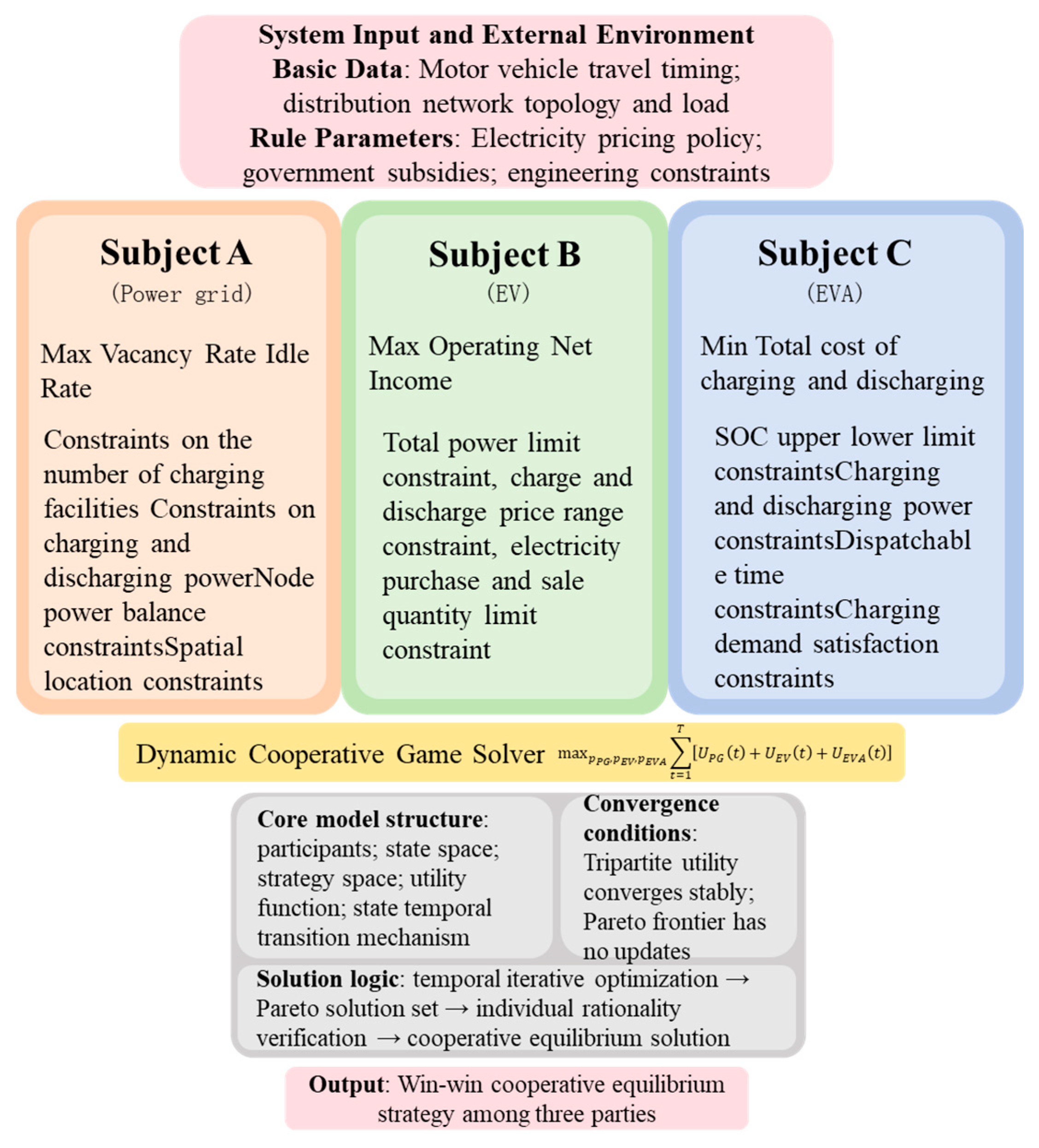
Most existing studies adopt static Stackelberg master–slave game models, which fail to capture the strong time-varying characteristics of EV charging demand and grid load [19]. Therefore, this paper constructs a three-party dynamic cooperative game model based on the Markov decision process (MDP), which takes 24 periods of the day as discrete time steps. In each time step, the three parties adjust the strategy according to the current system state and find the cooperative equilibrium solution that meets the collective rationality and individual rationality through dynamic iteration so as to realize the collaborative optimization of the interests of the three parties.

4.1. Mathematical Formalization Definition of Dynamic Game Based on MDP

In this paper, the tripartite dynamic cooperative game is defined as five tuples g = {N, S, A, P, R, γ}, in which the mathematical definitions of each element are outlined below.

4.1.1. Game Participant Set N

The participants in the game are the power grid, EV users, and the EVA, i.e., N = {Grid, EV, EVA}. The EV user group is aggregated by the EVA and participates in the game as a whole, avoiding the explosion of model complexity caused by decentralized individual decision-making.

4.1.2. System State Space S

The system state $s_t\in S$ represents all the core time-varying factors that affect the tripartite decision at time T. In this paper, the state vector is defined as

$$s_t=\left[\begin{array}{c}{L}_t,Q_t,{\overline{\mathrm{SOC}}}_t,{\overline{U}}_t\end{array}\right],$$

(24)

where $L_t\in {ℝ}^{+}$ is the total basic load power of distribution network at time t; $Q_t\in {ℝ}^{+}$ is the total charging demand power of regional EV at time, unit: kW; ${\overline{\mathrm{SOC}}}_t\in [0.2,0.9]$ is the average state of charge of all EVs connected to EVA at time; and ${\overline{U}}_t\in [0.9,1.1]$ is the unit value of the average node voltage of the distribution network at time t.

The state space s is the Cartesian product of the value ranges of the above four state variables, and all state variables can be collected in real-time through the power grid SCADA (Supervisory Control And Data Acquisition) system and EVA charging management platform.

4.1.3. Joint Action Space A

Joint action $a_t\in A$: This indicates the strategy combination adopted by the three parties at time t, i.e., $a_{\mathrm{Grid},t}=[C_{c,t},C_{d,t},N_{\mathrm{cha},t}]$. The action space of each subject is defined as follows:

(1) Grid-side action $a_{\mathrm{Grid},t}$, including time of use price adjustment and charging facility scheduling strategy, i.e., $a_{\mathrm{Grid},t}=[C_{c,t},C_{d,t},N_{\mathrm{cha},t}]$, where C_c,t, C_d,t is the charge and discharge price at time t, NCHA, and t is the number of charging facilities put into operation at time t.

(2) EV-user-side action $a_{\mathrm{EV},t}$: This refers to the charging and discharging power decision of a single EV, i.e., $a_{\mathrm{EV},t}={[P_{c,k,t},P_{d,k,t}]}_{k=1}^{N_{\mathrm{EV}}}$.

(3) EVA-side action $a_{\mathrm{EVA},t}$ is the power trading strategy with the grid, i.e., $a_{\mathrm{EVA},t}=[P_{\mathrm{grid},c,t},P_{\mathrm{grid},d,t}]$, where $P_{\mathrm{grid},c,t}$ and t are the power purchased from the grid and $P_{\mathrm{grid},d,t}$ is the power sold to the grid.

4.1.4. State Transition Probability P

The state transition probability represents the probability that the system will transition to state s_t+1 at time t after the system is in state s_t and the joint action a_t is executed. Based on historical data and physical laws, this paper decomposes the transition process of each state variable.

(1) Basic load transfer: The basic load of the power grid has a strong time-series correlation, which is modeled by a first-order Markov chain, and the transfer probability matrix is obtained from the statistics of historical load data.

(2) EV charging demand transfer: Based on the EV travel law generated by Monte Carlo simulation, the probability of EV access/departure at different times is counted, and the transfer probability of charging demand is obtained by combining the charging and discharging power decision.

(3) Average SOC transfer: Derived from the SOC update formula of all EVs, which is a deterministic transfer process.

(4) Node voltage transfer: Derived from the power flow Equation (11) of the distribution network, which is a deterministic transfer process.

To sum up, the overall state transition probability of the system can be expressed as the product of the transition probabilities of each state variable:

$$P(s_{t+1}|s_t,a_t)=P(L_{t+1}|L_t)\cdot P(Q_{t+1}|Q_t,a_t)\cdot P({\overline{\mathrm{SOC}}}_{t+1}|{\overline{\mathrm{SOC}}}_t,a_t)\cdot P({\overline{U}}_{t+1}|{\overline{U}}_t,a_t)$$

(25)

4.1.5. Immediate Reward Function R

The real-time reward function is the core bridge connecting the game model and the multi-objective optimization model. In this paper, the real-time rewards of the three parties are strictly bound with the objective function constructed above to achieve the unification of game benefits and optimization objectives.

(1) Grid-side instant rewards: The goal of the grid side is to minimize the charge shortage rate and facility idle rate, so the reward function is defined as the negative value of the objective function:

$$R_{\mathrm{Grid},t}(s_t,a_t)=-J_{1,t}(s_t,a_t),$$

(26)

where J₁ and t are the objective function values at the power grid side at time t. The greater the reward, the higher the power grid operation efficiency.

(2) EV-user-side instant rewards: The EV users’ goal is to minimize the full cost of charging and discharging, so the reward function is defined as

$$R_{\mathrm{EV},t}(s_t,a_t)=-J_{2,t}(s_t,a_t),$$

(27)

where J₂, t is the total charge and discharge cost of all EVs at time t. The greater the reward, the lower the user cost.

(3) EVA-side immediate reward: The EVA’s goal is to maximize operational revenue, so the reward function directly adopts its objective function:

$$R_{\mathrm{EVA},t}(s_t,a_t)=J_{3,t}(s_t,a_t),$$

(28)

where J₃, t is the operating income of the EVA at time t. The greater the reward, the higher the EVA’s income.

4.1.6. Discount Factor γ

The discount factor γ ∈ [0, 1] represents the weight of future revenue relative to current revenue. In this paper, γ = 0.95 is taken to reflect the priority of recent revenue in power system dispatching.

4.2. Cooperative Game Utility Function and Equilibrium Definition

4.2.1. Tripartite Utility Function

Under the MDP framework, the utility function of the game’s participants is defined as the mathematical expectation of the cumulative immediate rewards from time t to the end of the scheduling cycle T:

$$U_i(s_t)=\mathbb{E}[{\displaystyle \sum _{\tau =t}^T{\gamma }^{\tau -t}}{R}_{i,\tau }(s_{\tau },a_{\tau })|s_t],\hspace{1em}i\in N,$$

(29)

where $U_i(s_t)$ indicates that the participant i adopts the strategy sequence in the state S_t.${\left\{a_{\tau }\right\}}_{\tau =t}^T$ is the expected total utility that can be obtained.

4.2.2. Equilibrium Conditions of Cooperative Game

The equilibrium solution of the cooperative game should satisfy both collective rationality and individual rationality.

(1) Collective rationality:

There is no other joint strategy, so the utility of all participants is not reduced and the utility of at least one participant is strictly improved, that is, the equilibrium solution is the Pareto-optimal solution.

(2) Individual rationality:

The utility obtained by each participant through cooperation is not less than the maximum utility when they act alone, i.e.,

$$U_i^{*}\ge U_i^{\mathrm{non}-\mathrm{coop}},\hspace{1em}i\in N,$$

(30)

where $U_i^{*}$ is the utility of participant i under cooperative equilibrium, and $U_i^{\mathrm{non}-\mathrm{coop}}$ is the maximum utility of participant I when acting alone. In this paper, the solution satisfying the above two conditions is called the equilibrium solution of the tripartite cooperative game, and the set of all equilibrium solutions is the core of the cooperative game.

4.3. Refinement Constraints of Tripartite Policy Space

4.3.1. Electricity Price Strategy Space

The time of use price strategy at the grid side needs to reflect the impact of grid load and EV charging demand at the same time

$$P_t=a_t+b_t{L}_t+c_t{Q}_t,$$

(31)

where b_t and c_t are coefficients, lt is the load of the power grid at time t, and Qt is the predicted charging demand of electric vehicles at time t and can be understood as the basic electricity price part. The b_tL_t part reflects the adjustment of electricity price according to the grid load to guide users to stagger peak charging. The c_tQ_t part considers the impact of electric vehicle charging demand on electricity price. At the same time, the electricity price shall meet the following constraints:

$$P_{t,\min }\le P_t\le P_{t,\max },$$

(32)

where P_t,min and P_t,max are the lower limit and upper limit of electricity price at time t, respectively, which is determined by government policies, market competition, and other factors.

4.3.2. Charging and Discharging Participation Strategy

The charging and discharging participation strategy space is

$$S_{\mathrm{EV}2}=\left\{\right(q_{k,1}^{\mathrm{discharge}},q_{k,1}^{\mathrm{charge}}),\cdots ,(q_{k,\mathrm{T}}^{\mathrm{discharge}},q_{k,\mathrm{T}}^{\mathrm{charge}})\mid -q_{k,t,\max }^{\mathrm{discharge}}\le q_{k,t}^{\mathrm{discharge}}\le q_{k,t,\max }^{\mathrm{discharge}}\},$$

(33)

where $q_{k,t,\max }^{\mathrm{discharge}}$ is the maximum discharging power of the k-th user at time t (constrained by factors such as vehicle battery performance and safety); $q_{k,t,\max }^{\mathrm{charge}}$ is the maximum charging power (related to charging pile power, vehicle battery acceptance capacity, etc.).

Meanwhile, the battery SOC constraint must be satisfied, i.e.,

$${\mathrm{SOC}}_{k,\min }\le {\mathrm{SOC}}_{k,t}\le {\mathrm{SOC}}_{k,\max },$$

(34)

4.3.3. Trading Strategy with the Power Grid

Let $G_t^{\mathrm{buy}}$ denote the electricity quantity purchased by the EVA from the power grid at time t (where t = 1, 2,⋯, T and T is the total number of time periods in a day), and $G_t^{\mathrm{sell}}$ denotes the electricity quantity sold to the power grid.

The upper limit of the purchased electricity quantity is

$$G_t^{\mathrm{buy}}\le G_{t,\max }^{\mathrm{buy}},$$

(35)

where $G_t^{\mathrm{buy}}$ is the upper limit of the purchased electricity quantity.

The upper limit of the sold electricity quantity is

$$G_t^{\mathrm{sell}}\le G_{t,\max }^{\mathrm{sell}},$$

(36)

$G_{t,\max }^{\mathrm{sell}}$ is the total dischargeable electricity quantity of electric vehicles managed by the EVA.

4.4. Convergence Conditions of Cooperative Equilibrium

When the iterative process of the algorithm meets the following two conditions, it is considered to reach the equilibrium state of the tripartite cooperative game:

(1) Utility convergence conditions:

In successive k-generation iterations, the average utility changes in the three parties are less than the set threshold ε₁

$$\left|{\displaystyle \frac{U_i^{(g)}-U_i^{(g-K)}}{U_i^{(g-K)}}}\right|\le {\epsilon }_1,\hspace{1em}\forall i\in N,$$

(37)

which is the average utility of participant i in iteration g.

(2) Pareto front convergence condition:

In the continuous k-generation iteration, the number of non-dominated solutions of Pareto external file changes less than the set threshold ε₂

$$\left|N_{\mathrm{archive}}^{(g)}-N_{\mathrm{archive}}^{(g-K)}\right|\le {\epsilon }_2,$$

(38)

which is the number of solutions of Pareto external files in iteration g.

5. Multi-Objective CS Algorithm Combined with Game Theory

5.1. Cuckoo Search Algorithm

The standard multi-objective cuckoo search (MOCS) algorithm achieves performance complementarity through a dual-mode search mechanism. Local dimension: It generates local exploratory solutions via Levy flight in the neighborhood of the current optimal solution, enhancing the algorithm’s ability to conduct refined exploration of near-optimal regions. Global dimension: It constructs large-scale exploratory solutions through a far-field randomization strategy, ensuring the algorithm’s global optimization capability to escape local optima. However, the fixed assignment method of its discovery probability and step size parameters tends to cause slow convergence speed and reduced optimization accuracy of the algorithm. To address this defect, this paper adopts an improved multi-objective search algorithm (IMOCS) [20], which reconstructs the discovery probability and step size factor into dynamic functions of the number of iterations.

The improved position update formula of IMOCS algorithm is

$$x_i^{t+1}=x_i^t+{\rho }_i^t\oplus Le\nu y(\beta ),$$

(39)

In the formula, $x_i^t$ represents the position of the i-th cuckoo in the t-th generation; $\oplus$ is the step size factor, which determines the distance between the current solution and the optimal solution; Levy represents the use of the Levy flight strategy, which is employed to randomly explore a wider search space.

The improved search step size calculation formula is

$${\rho }_i^t={\rho }_{i,\min }^t+\left({\rho }_{i,\max }^t-{\rho }_{i,\min }^t\right)d_i^t,$$

(40)

$$d_i^t={\displaystyle \frac{x_i^t-x_{\mathrm{best}}^t}{{\max }_i\left|x_i^t-x_{\mathrm{best}}^t\right|}},$$

(41)

In the formula, ${\rho }_{i,\min }^t$ is the minimum value of the search step size; ${\rho }_{i,\max }^t$ is the maximum value of the search step size; $d_i^t$ is the improved dynamic step size factor. The calculation formula for the Levy flight factor remains unchanged, and is still

$$Le\nu y(\beta )={\displaystyle \frac{\varphi \mu }{{\left|\nu \right|}^{1/\beta }}},$$

(42)

$$\varphi ={\left[{\displaystyle \frac{\Gamma (1+\beta )\cdot \sin (\pi \beta /2)}{\Gamma \left(\frac{1+\beta }{2}\right)}}\right]}^{1/\beta },$$

(43)

In the formula, μ and v are random numbers following a normal distribution; β is usually set to 1; $\Gamma$ denotes the gamma function.

The improved discovery probability can be expressed as

$$p_{\mathrm{d}}(t)=p_{\mathrm{d},\max }-{\displaystyle \frac{t}{t_{\max }}}(p_{\mathrm{d},\max }-p_{\mathrm{d},\min }),$$

(44)

In the formula, $p_{\mathrm{d}}(t)$ represents the discovery probability in the t-th generation; $p_{\mathrm{d},\max }$ is the maximum value of the discovery probability; $p_{\mathrm{d},\min }$ is the minimum value of the discovery probability.

Therefore, the new solution for generation t+1 can be expressed as

$$x_i^{t+1}\left\{\begin{array}{cc}{x}_i^t+{\displaystyle \frac{{\rho }_0\varphi \mu }{{\left|\nu \right|}^{1/\beta }}}& \mathrm{rand}>p_{\mathrm{d}}\\ \varnothing & \mathrm{rand}\le p_{\mathrm{d}}\end{array}\right.,$$

(45)

In the formula, p_d is the probability that a cuckoo finds a new nest. It is generally set between 0.2 and 0.5, which can adjust the balance between local search and global search, and is usually taken as 0.2; “rand” is a random number that controls the decision of position update.

In multi-objective optimization algorithms, the global optimal solution guides the evolutionary direction of the population and must be selected from the non-dominated solutions in the external archive to balance convergence and diversity. Since these two objectives (convergence and diversity) are conflicting, it is necessary to evaluate the convergence and diversity of solutions in separate dimensions.

This paper adopts the dominance strength method to select the global Pareto-optimal solution. This method takes the total number of objective dominance times of a solution over other solutions as the ranking criterion, which objectively reflects the comprehensive degree to which a solution approaches the true Pareto front. After sorting the solutions in descending order of dominance strength, the solution with the smallest sequence number is selected as the optimal solution. The calculation formula for dominance strength is as follows:

$$d{s}_i={\displaystyle \sum _{k=1}^{K}d}{o}_{i,k},$$

(46)

In the formula, do_i,k represents the total dominance count of the i-th solution over other solutions with respect to the k-th objective function.

5.2. Overall Optimization Process

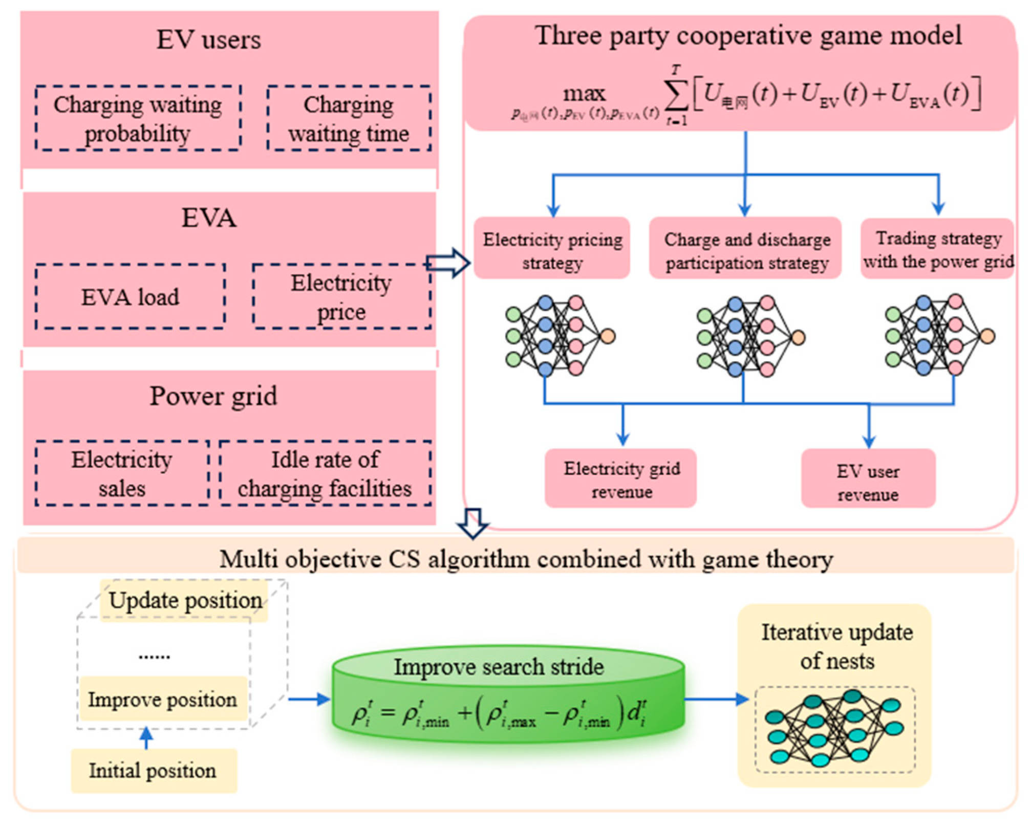
Figure 1 illustrates the process of charging and discharging optimization among the power grid, EVs, and EVA. First, relevant factors are considered from three perspectives: EV users, the power grid, and the EVA. EV users focus on the probability and duration of charging waiting; the power grid focuses on the electricity sales volume and idle rate of charging facilities; and the EV aggregators focus on EVA load and charging/discharging prices.

Subsequently, the EVA charging and discharging optimization model of grid electric vehicles is constructed, as shown in Figure 2 below. On this basis, an optimization algorithm combining game theory and the CS algorithm is applied. This algorithm consists of two core processes: an iterative search process (including initialization, Levy flight search, and abandoning/updating nests) and a cooperative game process (including the iteration process, convergence conditions, and equilibrium achievement). Finally, a V2G optimization strategy from the perspective of a multi-party cooperative game and based on the CS optimization algorithm is obtained.

The algorithm process shown in Algorithm 1 first initializes core parameters, including population size, maximum number of iterations, step size bounds, discovery probability bounds, Lévy index, convergence thresholds, and an empty Pareto external archive. The algorithm randomly generates n cuckoo individuals coded as joint strategies in the three-party joint strategy space, calculates their objective function values, and stores the non-dominated solutions in the file after non-dominated sorting. If the file size exceeds the upper limit, the solution with less crowded degree is deleted by the crowding degree distance method to maintain population diversity. It then enters the iteration cycle. Each generation first dynamically calculates and updates the search step size and discovery probability according to the current iteration times, updates the Levi flight position for all individuals, and calculates the objective function value of the new individual. It then judges and discards the inferior solution by generating the random number in the [0, 1] interval and randomly generates new individuals. After completing the population update, it compares the new individual with the archive solution to update the Pareto external archive; when the maximum number of iterations is reached or there is no significant update of the non-dominated solution in the archives for ten consecutive generations, the algorithm converges. Finally, by calculating the dominant strength of each solution in the archives, the solution with the largest dominant strength is selected as the optimal equilibrium strategy of the tripartite cooperative game.

Algorithm 1: Three party cooperative game equilibrium solving algorithm based on IMOCS

Input: population size n, maximum iteration times t_max, α_max, α_min, p_dmax, p_dmin, λ Output: optimal cooperative equilibrium strategy a* 1: Initialize Pareto external file archive = ∅ 2: Random initialization population x = {x_1, x_2,..., x_n} 3: Calculate the objective function value of each individual f (x_i) = [j1 (x_i), J2 (x_i), J3 (x_i)] 4: Non dominated sorting x, adding non dominated solutions to archive 5: for t = 1 to T_max do 6: Calculate dynamic step α (T) = α_min + (α_max − α_min) *exp (−5* (t/t_max) ^2) 7: Calculate the dynamic discovery probability p_d (T) = p_dmax − (p_dmax-p_dmin) * (t/t_max) 8:   for i = 1 to N do 9: Generate Levy flight step L (λ) 10:     x_new = x_i + α(t) ⊕ L(λ) 11: Calculate f (x_new) 12:     if rand > p_d(t) then 13:         x_i = x_new 14:     else 15: X_i = randomly generate new individuals 16:     end if 17:    end for 18: Non dominated sorting x ∪ archive, update Archive 19: If the convergence condition satisfies then 20:     break 21:    end if 22: end for 23: calculate the dominant strength of each solution in archive doi_i 24: a* = argmax(DOI_i) 25: return a*

6. Case Study Analysis

6.1. Example Parameters

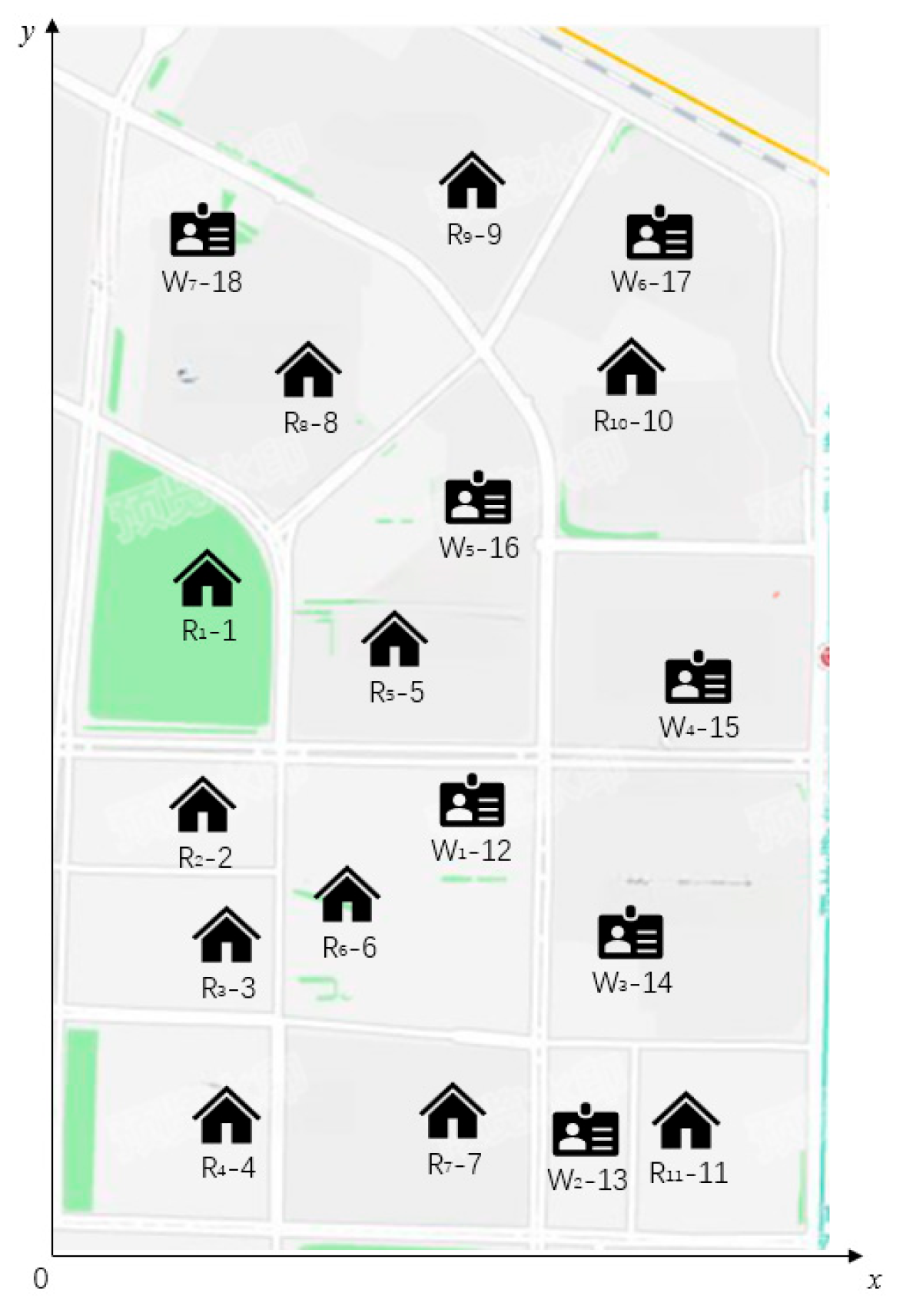
The test scenario is shown in Figure 3. The distribution network topology of this area consists of seven feeders (L1–L7) with a voltage level of 10 kV, each with a maximum current-carrying capacity of 480 A. Electricity is supplied by three upper-level substations (S1–S3). There are 18 load nodes in the area, among which 11 are residential nodes (R1–R11) and 7 are work nodes (W1–W7). The load at each node is closely related to the charging demand of EV users, and these demands change with time and EV charging scheduling strategies. To accurately reflect the time-varying nature of grid load, we assume that EV charging demand fluctuates significantly across different time periods—particularly during peak hours when EV users return home collectively and depart in the morning.

To enable grid load management to adapt to the time-varying characteristics of EV charging demand, we introduce the proposed tripartite dynamic cooperative game model. The charging decisions of EV users are influenced not only by electricity prices, but also by grid load management. Grid operators optimize scheduling to meet these demands, thereby ensuring stable grid operation and preventing overload.

In this study, we consider how EV charging demand changes over time. Through simulating charging demand predictions for different time periods, we adjust the grid’s scheduling strategy. This time-varying characteristic is particularly critical to the topological parameters of the test area, as the peak periods of EV charging demand are closely linked to the time-dependent fluctuations of grid load. Therefore, the location and number of charging facilities must be optimized based on demand changes during these periods.

The maximum north–south distance of the area is 33 km, and the maximum east–west distance is 30 km. In the figure, solid lines represent transmission lines, while dashed lines represent traffic routes. Based on the EV penetration rate and population data of this area, the expected number of EVs in ownership is approximately 1235. The spatiotemporal distribution of charging demand is derived using a time-period prediction model. Before the construction of EV charging stations, each load node was equipped with low-power charging facilities with a power rating of 7 kW. According to the EV-to-charging-pile ratio (approximately 3:1), the total number of charging facilities is about 376, meaning an average of 19 charging facilities per load node.

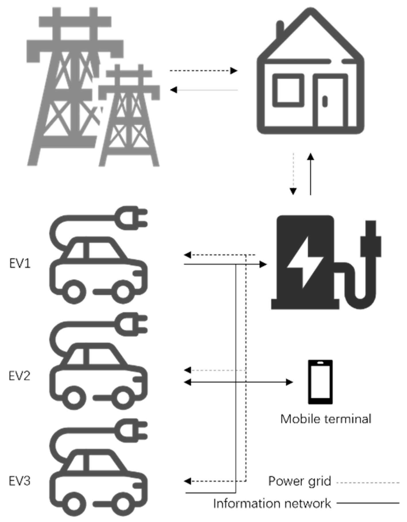
In scenarios where EVs queue for charging, each charging facility can serve multiple vehicles, but only charges one vehicle at a time, following the “first-come, first-served” principle. When a vehicle’s charging demand is met, charging is interrupted, and the next vehicle starts charging immediately. Charging information is uploaded to the cloud in real-time, allowing vehicle owners to check the information via their mobile phones and select a suitable charging location. If the charging facilities at the nearest location are fully occupied, owners can choose other locations. It is assumed that the service radius of each EV charging station is 5 km, and the rated power of each charging facility within a station is 30 kW. The scenario of electric vehicles queuing for charging is shown in Figure 4.

The optimization variables include the abscissa, ordinate, and number of charging facilities of the charging station. The value ranges of the abscissa and ordinate are [0, 30] and [0, 33], respectively, using the unit of kilometers. The lower limit of the number of charging facilities is zero, and the upper limit is the maximum access number corresponding to the system’s static voltage margin. This algorithm is implemented in Matlab 2018b software, with an overall calculation time of approximately 40 min.

6.2. Optimal Solution Selection

During the optimization process, a dynamic game model was adopted to balance the interests of three parties: EV users, charging station investors, and power grid operators. In this game model, the charging decisions of EV users are influenced by grid load management and electricity pricing strategies, while the scheduling decisions of grid operators are based on fluctuations in EV charging demand and the real-time usage status of charging facilities.

Through the cooperative game method, the finally obtained Pareto-optimal solution set provides an optimal interest balance among EV users, the power grid, and grid operators. To determine the optimal scheme, the optimization variables of charging stations (the location and number of charging facilities) were combined with the grid load changes within the time period, and the dynamic game model was used to analyze the advantages and disadvantages of different schemes. Ultimately, Solution 1, with a dominance strength of 24, was selected as the optimal solution. This scheme not only effectively covers 6 load nodes, but also ensures the stable operation of the power grid and optimizes the utilization rate of charging facilities and the balance of grid load.

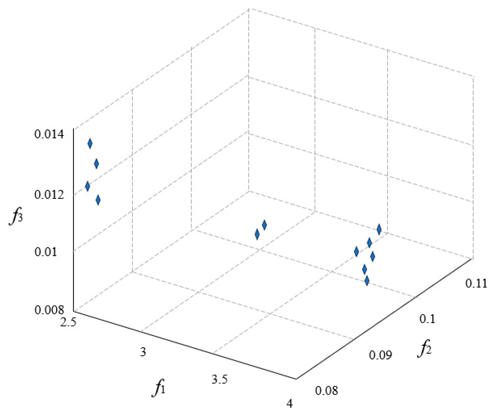
The 3D distribution of the finally obtained Pareto-optimal solution set is shown in Figure 5, which contains a total of 13 solutions. Among them, Solutions 1–13 are non-dominated by each other. The values of optimization variables and objective functions are listed in Table 2. Since these solutions are non-dominated, it is necessary to evaluate the priority of each solution using the dominance strength rule: the greater the dominance strength, the higher the priority. The results show that Solution 1 has the highest dominance strength of 24 and thus the highest priority; therefore, Solution 1 is selected as the optimal solution. The charging station location corresponding to Solution 1 is (20, 15), which covers six load nodes (nodes 5, 9, 10, 11, 13, 16, and 17), with a total of 39 charging piles.

6.3. Optimization Result Analysis

This section mainly analyzes the changes in various evaluation indicators before and after the optimization of EV charging station planning. These indicators include the charging waiting time and waiting probability for EV users, the charging volume deficit rate and idle rate of charging facilities, as well as the average line load rate and static voltage stability index of the distribution network.

(1) Charging waiting time and waiting probability of electric vehicle users

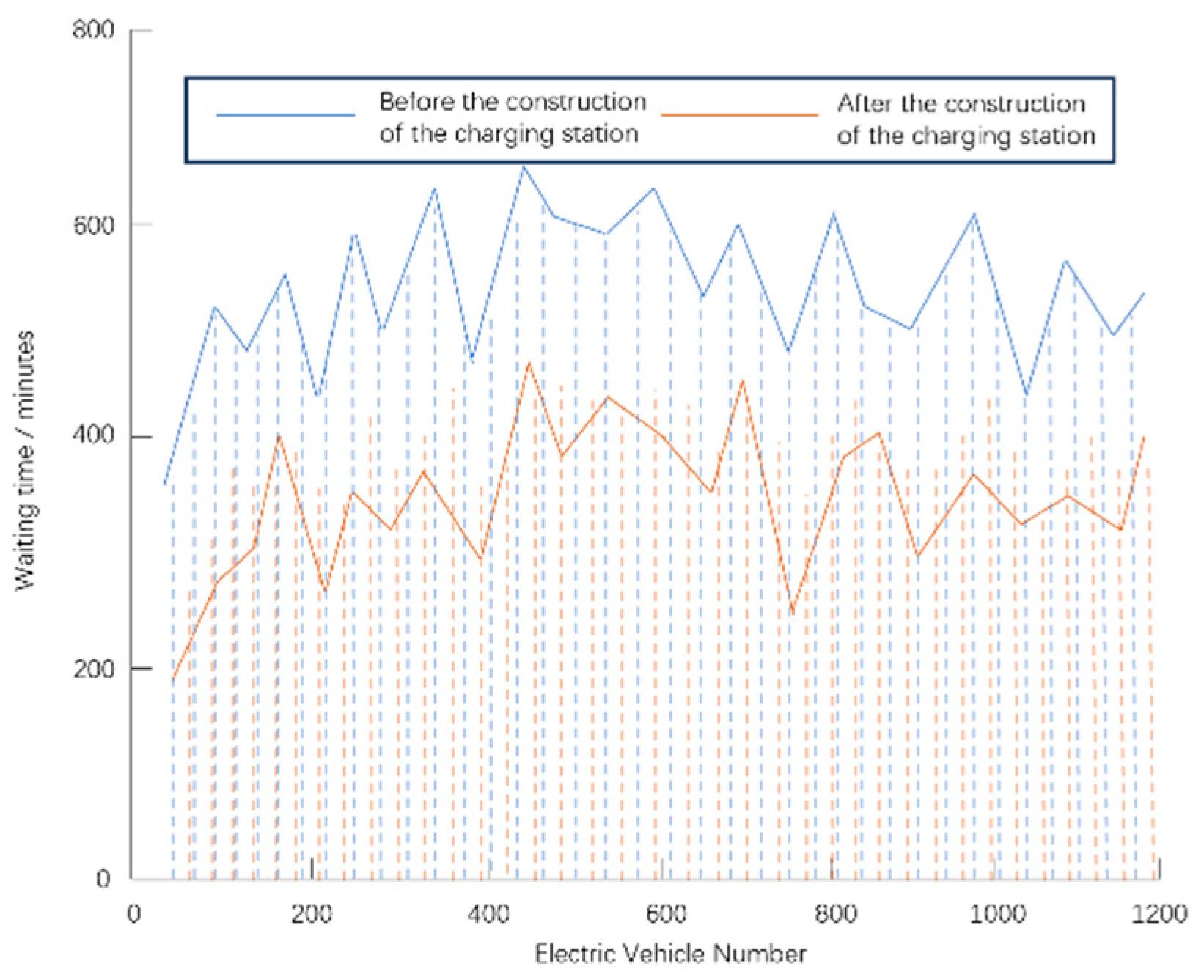
The waiting time for electric vehicle charging is shown in Figure 6. After the completion of the charging station construction, the waiting time for most vehicles significantly decreased. Specifically, the average waiting duration dropped from 394 min (before construction) to 269 min, representing a notable reduction. Within the service coverage area of the charging stations, some EV users prioritize charging their vehicles at these stations; this choice alleviated the queuing situation at certain charging nodes, thereby lowering the overall average charging waiting duration. The simulation results indicate that, after the optimization of charging station planning, the number of EVs with reduced charging waiting duration reached 801, which fully demonstrates the positive role of charging station construction in improving users’ charging efficiency.

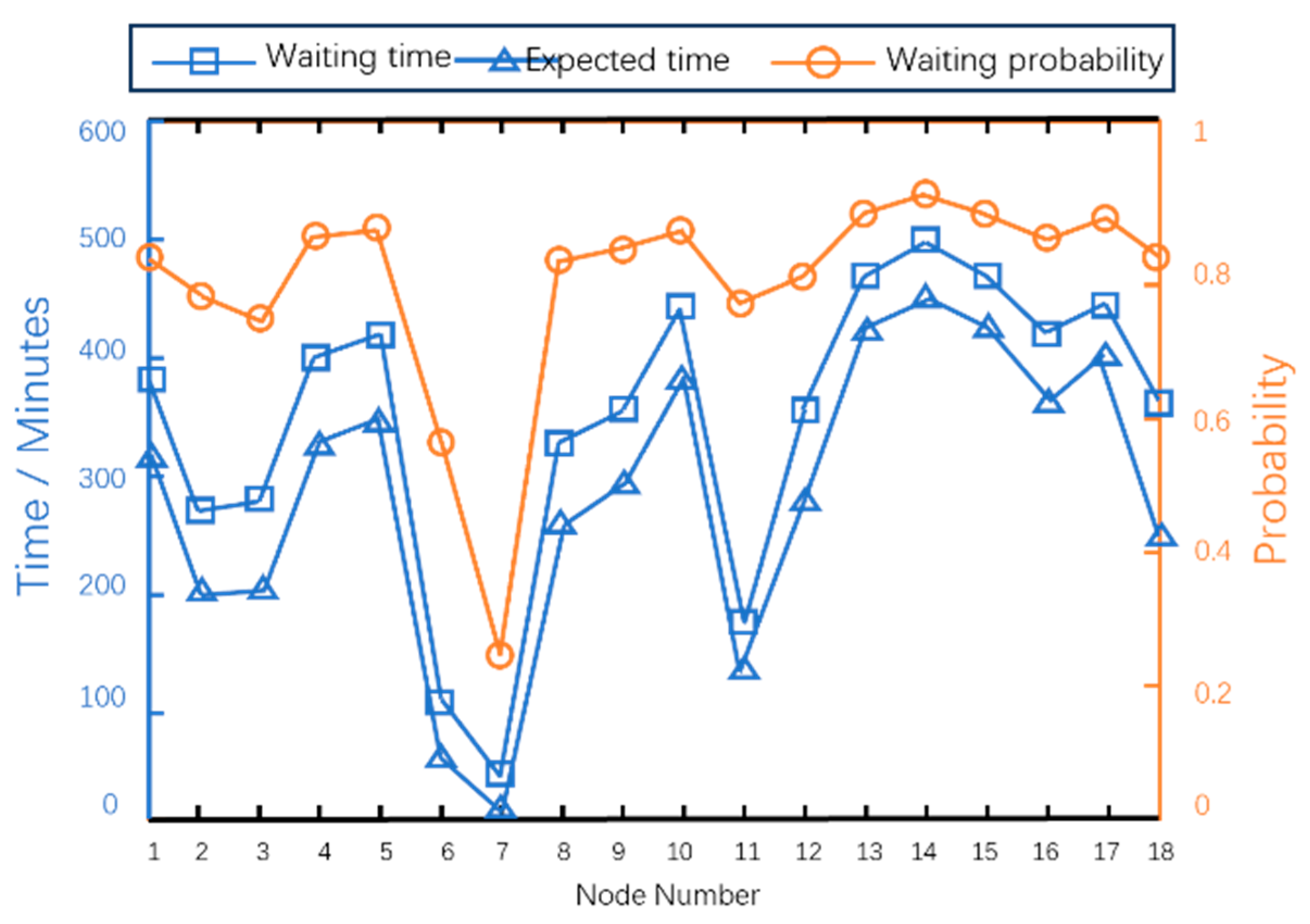
By analyzing the distribution data of charging waiting time at nodes as shown in the figure below, it can be seen that there are differences in charging waiting time of electric vehicles at different nodes. Taking node 2 and node 3 as examples, their charging waiting durations are 274 min and 281 min, with corresponding waiting probabilities of 0.74 and 0.72, respectively. Although the waiting duration and probability values of these two nodes differ, the calculated waiting time cost for both is 207 min.

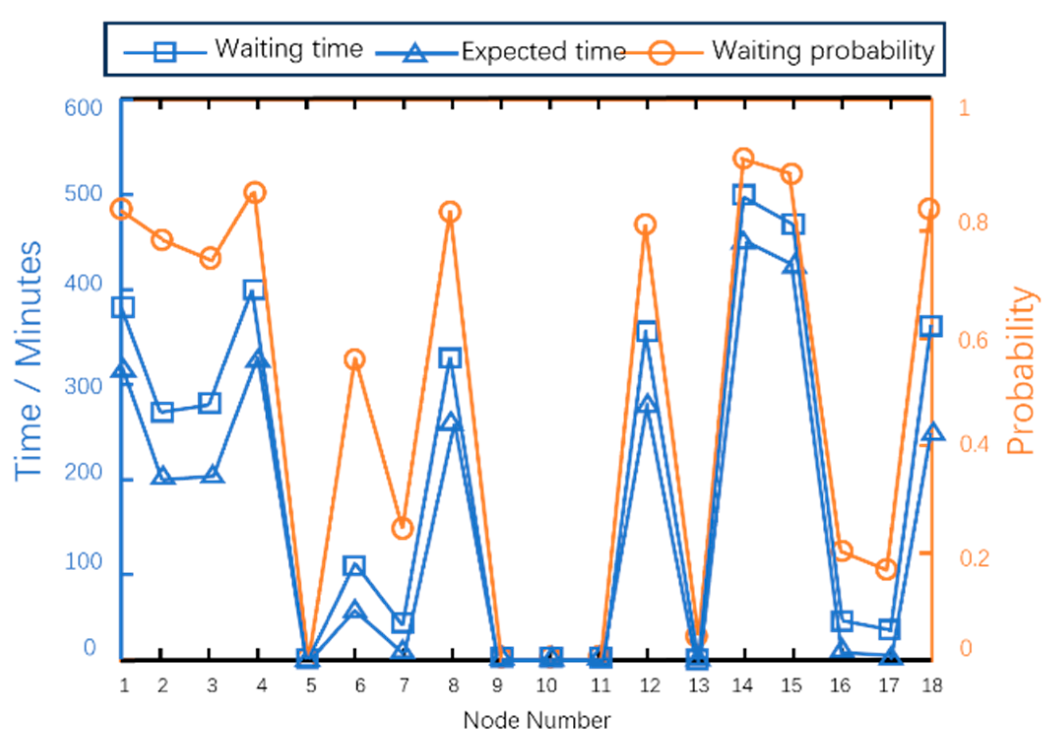
Comparing Figure 7 and Figure 8, before the charging stations were put into use, the charging waiting probabilities of nodes 5, 8, 9, 10, 11, 13, and 16 were all higher than 0.6 and the average waiting time cost of the nodes reached 288 min; after the charging stations were built, the waiting probabilities of the aforementioned nodes all dropped to zero, and the average waiting time cost decreased to 163 min accordingly. This data change intuitively indicates that, for nodes within the service range of the charging stations, their charging waiting time cost significantly reduced, and the overall charging congestion of the system is notably alleviated.

(2) Arrival and loss of electric vehicle users

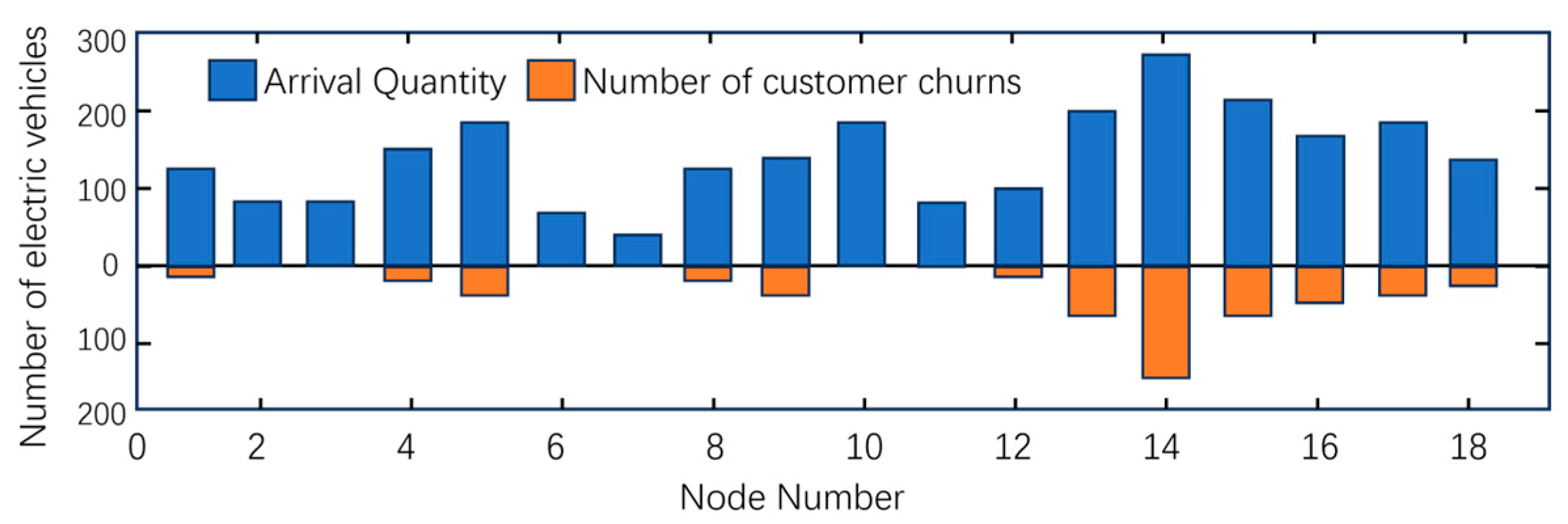
The distribution of the number of electric vehicles arriving at nodes and the number of customer losses before the construction of charging stations is shown in Figure 9. When an EV arrives at a charging node, if it cannot connect to the power grid for charging due to the continuous busyness of charging equipment, the user’s willingness to choose this node for charging in the future will decrease, which in turn leads to customer loss at this node. From the perspective of the distribution of EV arrival volume and user loss volume at nodes, before the construction of charging stations, the number of lost customers reached 609, accounting for approximately 49.8% of the total number of EV users. Among them, the customer churn rates at residential nodes and work nodes were 11.6% and 40.7%, respectively, indicating that the loss problem at work nodes was significantly more prominent. This is because, compared with work nodes, users at residential nodes have longer parking durations and more sufficient charging facility configurations, which provides EVs with more opportunities to charge.

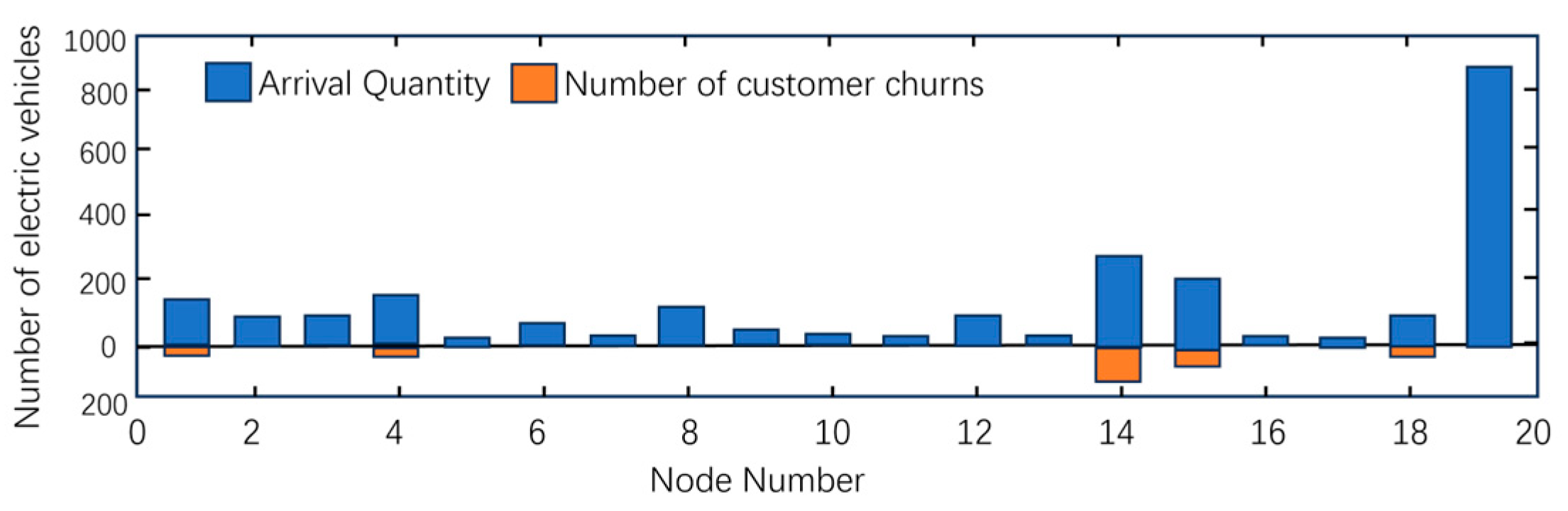
The distribution of the number of electric vehicles arriving at nodes and the number of customer losses after the construction of charging stations is shown in Figure 10. After the charging stations were built, the number of lost customers decreased from 609 to 318, and the customer churn rate dropped from 49.8% to 19.6%. The clear changes in the data indicate that the planning scheme effectively alleviated the problem of customer loss caused by insufficient supply of charging facilities and significantly improved the service attractiveness of charging nodes.

6.4. Comparison of Different Optimization Algorithms

Table 1 and Table 2 below present a comparison of the results of different optimization algorithms. The optimal solutions of the multi-objective CS algorithm before improvement and the Particle Swarm Optimization (PSO) algorithm are (20, 15, 60) and (20, 14, 45), respectively. After these solutions are incorporated into the Pareto-optimal solution set obtained by the method proposed in this paper, the dominance strength method is adopted to rank the priority of each solution. The results show that the dominance strengths of these two solutions are 24 and 22, their priorities are 3 and 4, and the number of nodes they cover is 7 and 5, respectively. The optimal solution based on the linear weighted sum method is (20, 14, 51), with a dominance strength of 22, a priority rank of 4, and coverage of 5 nodes.

The comparison results show that the proposed method outperforms the other three algorithms in all key metrics: it covers the maximum number of nodes, achieves the highest dominance strength of 26, and ranks first in priority.

Table 1. Objective function values and priority distributions of different solutions.

Solution Number	X1	X2	X3	f1	f2	f3	Dominant Strength	Priority
1	18	16	38	2.60	0.0785	0.0112	24	1
2	19	16	42	2.62	0.0788	0.0115	23	2
3	21	14	43	2.58	0.0792	0.0128	21	3
4	22	13	45	2.59	0.0790	0.0135	21	3
5	24	15	32	3.51	0.0995	0.0102	20	4
6	22	16	49	3.46	0.1020	0.0097	19	5
7	23	15	46	3.79	0.1074	0.0098	16	6
8	23	14	49	3.75	0.1122	0.0097	15	7
9	26	14	48	3.95	0.1064	0.0098	15	7
10	25	14	99	3.90	0.1075	0.0085	15	7
11	26	13	1	3.92	0.1072	0.0092	14	8
12	25	15	82	3.92	0.1079	0.0089	13	9
13	27	15	92	3.90	0.1072	0.0086	13	9

Table 1. Objective function values and priority distributions of different solutions.

Solution Number	X1	X2	X3	f1	f2	f3	Dominant Strength	Priority
1	18	16	38	2.60	0.0785	0.0112	24	1
2	19	16	42	2.62	0.0788	0.0115	23	2
3	21	14	43	2.58	0.0792	0.0128	21	3
4	22	13	45	2.59	0.0790	0.0135	21	3
5	24	15	32	3.51	0.0995	0.0102	20	4
6	22	16	49	3.46	0.1020	0.0097	19	5
7	23	15	46	3.79	0.1074	0.0098	16	6
8	23	14	49	3.75	0.1122	0.0097	15	7
9	26	14	48	3.95	0.1064	0.0098	15	7
10	25	14	99	3.90	0.1075	0.0085	15	7
11	26	13	1	3.92	0.1072	0.0092	14	8
12	25	15	82	3.92	0.1079	0.0089	13	9
13	27	15	92	3.90	0.1072	0.0086	13	9

Table 2. Comparison of optimal solutions of different optimization algorithms.

Optimization Algorithm	Optimal Solution	Objective Function Value	Dominant Strength	Priority	Covering Nodes
MOCS	(18,16,58)	(2.58,0.0800,0.0125)	24	3	5,9,10,11,13,16,17
This algorithm	(22,14,38)	(2.62,0.0785,0.0112)	26	1	5,9,10,11,13,16,17
MOPSO	(21,15,44)	(3.15,0.0880,0.0102)	22	4	5,11,13,16,17
LWS	(20,13,51)	(3.12,0.0885,0.0103)	22	4	5,11,13,16,17

Table 2. Comparison of optimal solutions of different optimization algorithms.

Optimization Algorithm	Optimal Solution	Objective Function Value	Dominant Strength	Priority	Covering Nodes
MOCS	(18,16,58)	(2.58,0.0800,0.0125)	24	3	5,9,10,11,13,16,17
This algorithm	(22,14,38)	(2.62,0.0785,0.0112)	26	1	5,9,10,11,13,16,17
MOPSO	(21,15,44)	(3.15,0.0880,0.0102)	22	4	5,11,13,16,17
LWS	(20,13,51)	(3.12,0.0885,0.0103)	22	4	5,11,13,16,17

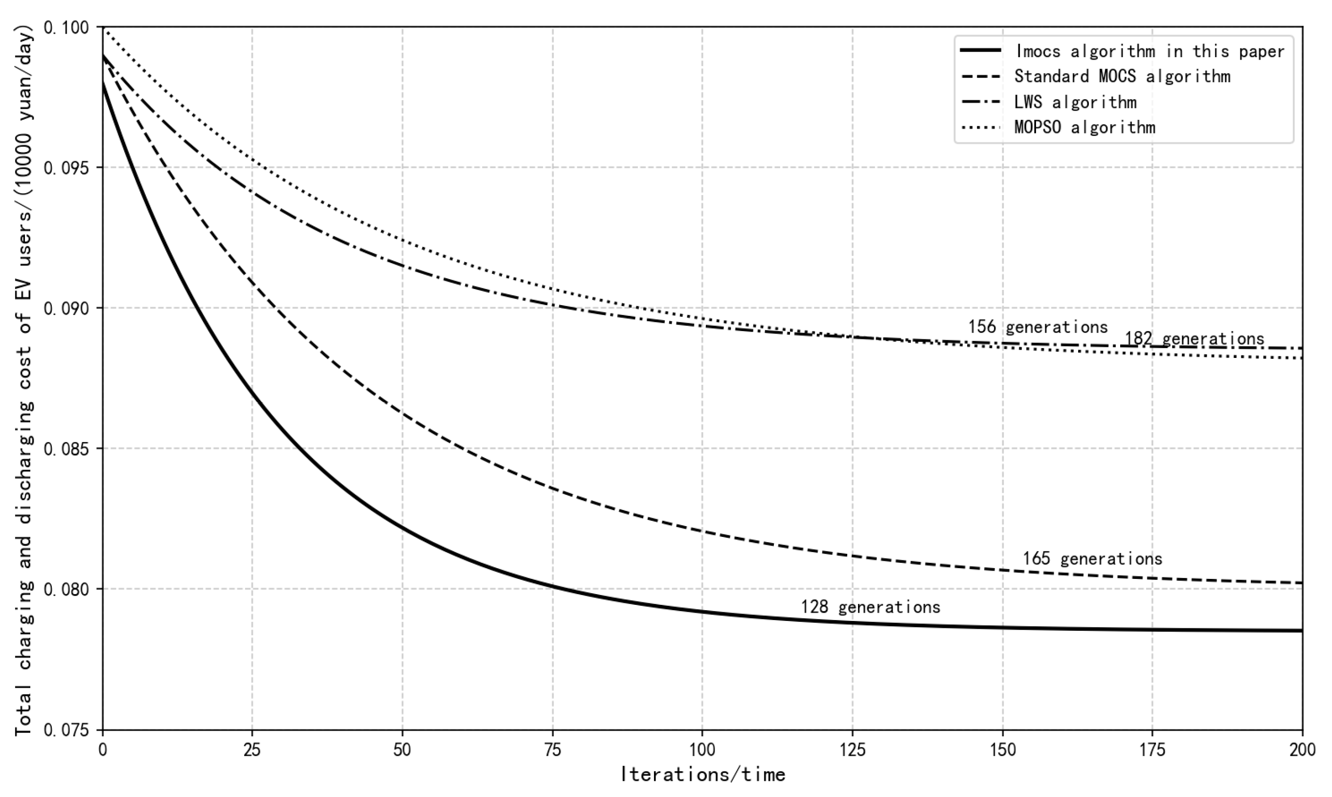
The comparison of convergence curves of different algorithms is shown in Figure 11. As can be seen from the figure, the IMOCS algorithm in this paper has entered the rapid convergence stage in about 80 generations of iterations and fully converged in 128 generations, while the standard MOCS only entered the convergence stage at about 120 generations and the 165 generations were fully convergent; MOPSO (Multi-Objective Particle Swarm Optimization) and LWS (Linear Weighted Sum) need more than 150 generations to converge. This is because the improvement in dynamic step size and dynamic discovery probability enables the algorithm to quickly explore the solution space at the early stage of iteration and fine search the optimal solution at the late stage of iteration, effectively balancing the global exploration and local development capabilities. At the same time, the objective function value of this algorithm is the lowest after convergence, which shows that its optimization accuracy is significantly better than the other three algorithms.

6.5. Robustness Analysis

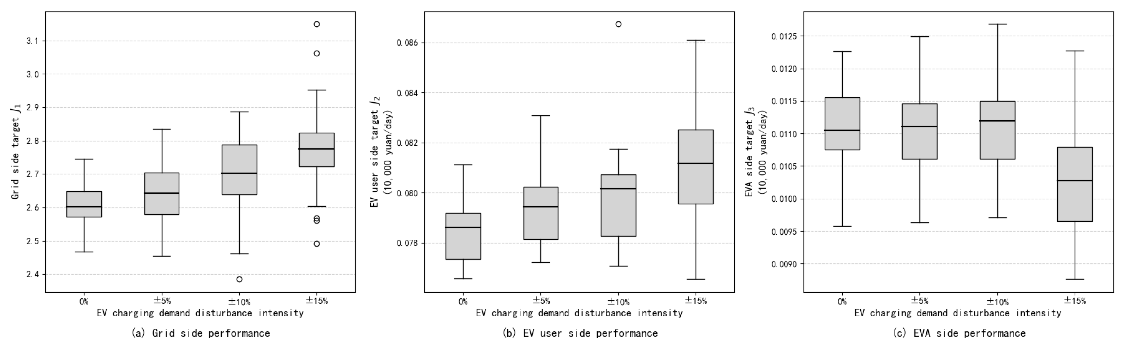
In order to further verify the robustness of the proposed algorithm, a test was carried out under the scenario of EV charging demand with random fluctuations of ±5%, ±10%, and ±15%, and the results are shown in Figure 12. It can be seen from the figure that, as the disturbance intensity increases, the values of the three objective functions only deteriorate slightly, and the box width (standard deviation) remains within a small range without obvious abnormal values. This shows that the IMOCS algorithm proposed in this paper has good adaptability to the random disturbance of key parameters, can run stably in the actual engineering scene, and has strong robustness.

7. Conclusions

This paper proposes a V2G optimization strategy based on the perspective of a multi-party cooperative game and the CS algorithm. By analyzing the interest demands of EV users, the power grid, and grid operators, relevant models are constructed. A cooperative game structure model for the three parties is defined, with its dynamic characteristics, strategy space, and payoff functions clearly specified. Leveraging the advantages of the improved CS algorithm, an iterative search and cooperative game are conducted. Through case study analysis, this strategy can balance the interests of the three parties; the solution obtained by the proposed algorithm is superior to that of other algorithms. This research provides a scientific basis for the planning of EV charging stations and contributes to maximizing the interests of all parties and ensuring the stable operation of the power grid.