A Coordinated Steady-State Optimization and Dynamic Control Scheme for Dual-Inverter OW-PMSM Drive Systems Focusing on Power Allocation

Abstract

The dual-inverter open-winding permanent magnet synchronous motor (OW-PMSM) drive system exhibits significant advantages for electric vehicles with dual energy sources, particularly in achieving coordinated energy management and efficient power allocation between the sources. Based on the dual-inverter OW-PMSM drive configuration, this paper proposes two stator current planning algorithms: one aims to minimize the electrical losses during motor operation and the other aims to maximize the power allocation range of the dual inverters, respectively. Building upon this, a geometric algorithm for stator voltage vector allocation is proposed to achieve smooth switching of the motor between the two algorithms. This enhances the tracking performance of the electromagnetic torque and d-axis current during motor operation, while ensuring that the motor operates within its steady-state range, thereby improving system stability. Finally, simulations and experiments are conducted on the proposed algorithm to verify its feasibility and advantages.

1. Introduction

Equipped with dual energy sources, electric vehicles demonstrate significantly improved energy utilization efficiency and driving reliability, meeting the demands of energy management under complex operating conditions. Among existing dual-source topologies, most schemes employ DC-DC converters to connect two different DC buses. Regarding the integration of dual energy sources, various power electronic interface solutions have been proposed in existing research. For instance, Reference [1] constructed a photovoltaic battery–supercapacitor dual energy storage system, where the battery and supercapacitor are connected to the DC bus through independent bidirectional DC-DC converters to supply power to the permanent magnet synchronous motor. Reference [2] designed a novel bidirectional DC-DC converter capable of achieving bidirectional power exchange between the two energy sources and the high-voltage DC bus. Furthermore, Reference [3] proposed three non-isolated dual-source DC-DC converter topologies to suit different operational requirements. These schemes essentially connect two DC buses by adding an extra power conversion stage, which relies on high-frequency switching devices and passive energy storage components. This results in relatively low energy transfer efficiency, and the energy management strategy is difficult to coordinate deeply with the high-speed dynamic control of the motor, thus limiting the overall energy management performance of the vehicle. 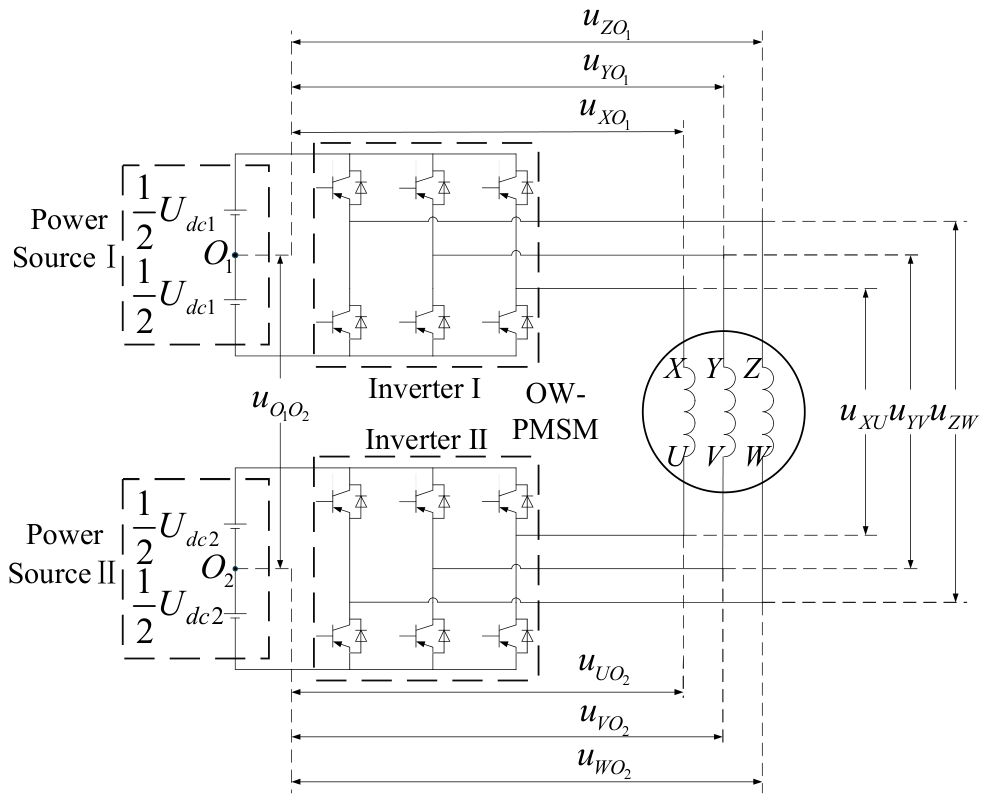Recent progress in energy storage technologies and their coordinated utilization highlights the importance of efficient power allocation in multi-source systems [4]. To address this issue, the dual-inverter open-winding motor topology is adopted. As shown in Figure 1, in this configuration, both ends of the stator windings are connected to voltage source inverters in series, opening the star connection point of the motor. The two voltage source inverters receive DC bus voltages from two isolated energy sources, respectively, and the DC buses of the two inverters are isolated from each other. References [5,6] also utilize this drive configuration.

Under this configuration, the work can be broadly divided into two mainstream directions. One of these is stator current optimization. Reference [7] introduced an algorithm for improving steady-state efficiency by incorporating a current distribution coefficient into the motor equivalent circuit that considers iron loss. Through analysis, the dq-axis currents at which loss is minimized are obtained, and then the electrical losses during steady-state motor operation are reduced through reasonable distribution. Reference [8] proposed an efficient optimization method based on an improved gradient descent algorithm within a discretized search space. A motor drive efficient configuration encompassing all losses of the inverter and the motor was established, eliminating the need to rely on a loss model. An improved gradient descent algorithm is used for current angle optimization. The algorithm searches for the optimal current angle under given constraints to maximize the efficiency of the drive system. Reference [9] proposed a full-region optimal mapping method based on a data-driven black-box configuration. The Nelder–Mead simplex (NMS) algorithm was improved to reduce the probability of optimization failure. A wide-temperature-range torque mapping is used to compensate for torque deviation and the optimal current angle, enabling the motor to achieve better efficiency performance across a wide temperature range.

The other direction is dynamic control during motor operation. Reference [10] proposed a configurable predictive current control with independent cost functions. Two independent cost functions are designed for the current errors of the d-axis and q-axis, forming a feasible region of rectangular voltage vectors. Subsequently, the voltage vector is solved with the objectives of optimizing switching frequency and current ripple. This method achieves independent adjustment of dq-axis current performance without requiring weighting factors, while also reducing inverter switching losses. Reference [11] proposed a multi-rate continuous control set configuration predictive control algorithm. Instead of solving a high-dimensional sequence of voltage vectors, the flux tracking process is divided into three stages: catching-up, transition, and holding. It offers better steady-state harmonic performance and eliminates overshoot during transients, ensuring both fast dynamic response and improved steady-state performance. Reference [12] proposed a cascade-free modulated predictive direct speed control. A second order sliding mode observer is used for speed prediction, and a dual-objective cost function considering both speed and current tracking is designed. Finally, the voltage vector solution under the existing constraints is derived. This method enables the system to achieve a fixed switching frequency, further enhancing its steady-state performance. In reference [13], a dual adaptive sliding mode control (SMC) scheme is proposed, which integrates robust mechanical parameter identification using adaptive sliding mode with adaptive sliding mode speed control. The observed total disturbance is directly used as the real-time load torque, endowing the algorithm with a feedforward control effect. This scheme not only enhances the system’s robustness underload disturbances but also eliminates the inherent chattering problem of SMC.

Building upon dynamic control, power allocation between the dual inverters can be achieved. Reference [5] previously utilized this structure; through dual power coordinated control, decoupling of active and reactive power is achieved based on PQ-axis coordinate transformation, thereby controlling the power distribution between the dual inverters. This paper broadens the dual-voltage configuration, where the dual energy sources output two DC bus voltages to the two inverters. The electric drive configuration under this structure integrates a power allocation module and an energy conversion module, enabling power distribution for the dual energy sources through the dual-inverter architecture and upper-level control strategies. The foundational framework of Reference [14] is similar. Based on a multi-source inverter-fed permanent magnet synchronous motor drive system, it proposes a power allocation strategy using a three-dimensional vector cube decomposition. This method decomposes a non-uniform three-dimensional vector cube into two symmetric sub-cubes and achieves power distribution by adjusting the decomposition coefficient. For other models, an active power allocation algorithm without DC-DC conversion was proposed in [15] based on a dual-winding motor.

For dual-inverter OW-PMSM drive systems, other relevant research mainly focuses on the following three directions: advanced topologies and control techniques for dual-inverter and OW-PMSM drives, modern traction inverter technologies, and advanced control and energy management strategies for multi-source electric vehicle powertrains. In the area of advanced topologies and control techniques for dual-inverter and OW-PMSM drives, Reference [16] improves conventional predictive current control and proposes a dual-vector predictive current control with zero-sequence current hysteresis. It simplifies the candidate vector selection and action time calculation, utilizes the switching state redundancy of the dual-inverter system to achieve zero-sequence current hysteresis suppression, realizes zero-sequence suppression independent of the motor model, and simultaneously reduces high-speed current harmonics. Regarding modern traction inverter technologies, Reference [17] designed a high-precision modulation scheme for different DC voltage ratios. The high-voltage side inverter uses clamped low-frequency operation, while the low-voltage side employs high-frequency SVPWM, reducing current harmonics and improving control accuracy. For advanced control and energy management strategies in multi-source electric vehicle powertrains, Reference [18] focuses on power distribution among multiple energy sources and proposes a model predictive control based on an energy management strategy and dual reinforcement learning. It uses a neural network for vehicle speed prediction and dual reinforcement learning for rolling optimization, thereby achieving global optimal energy loss.

In our previous work [6], two stator current planning algorithms were proposed, aiming to minimize efficiency losses during motor operation and to expand the power allocation range, respectively. Building on this, a composite sliding mode control algorithm was designed using electromagnetic torque and d-axis current as sliding surfaces, ensuring smooth switching between the two stator current planning algorithms. However, this prior work still has two main limitations: first, the proposed maximum voltage allocation algorithm did not consider the influence of the stator current on power, and therefore could not achieve the motor’s maximum power allocation range; second, when the motor’s operation exceeds its characteristic range, the proposed composite sliding mode control algorithm can lead to instability due to the limitation of the maximum allowable voltage amplitude.

Based on this, this paper takes an electric vehicle equipped with an isolated DC-bus dual-inverter OW-PMSM as the research object, conducting research on the steady-state optimization and dynamic control of the stator current. First, a dynamic model of the motor is established, and the feasible region for dual-inverter power allocation is analyzed. Second, two stator current planning algorithms are proposed, aimed at improving steady-state efficiency and expanding power allocation capability, respectively. Compared with previous work, instead of simply pursuing the maximum power allocation range by minimizing the stator voltage vector amplitude, the proposed approach comprehensively determines the maximum power allocation range via a linearized formulation, taking into account the projection amplitude of the current in the voltage direction. On this basis, a novel stator voltage vector allocation scheme is designed to achieve transient control of motor torque and current, optimizing the dynamic response of the stator current while ensuring stable tracking of the electromagnetic torque.

The structure of this paper is organized as follows: Section 2 establishes the mathematical configuration of the system and analyzes the feasible region for inverter power allocation. Section 3 proposes two steady-state stator current planning algorithms. In Section 4, a parallelogram-based scheme is proposed to optimize the torque and current tracking requirements during motor operation. Section 5 validates the feasibility of the proposed scheme through both simulation and experimental comparisons with a decoupled PI control strategy. Finally, Section 6 concludes the paper.

2. System Modeling and Feasible Region Analysis

2.1. Dynamic Modeling and Analysis of the OW-PMSM

The model analysis in this section is based on the following assumptions: symmetry of the three-phase windings, sinusoidal distribution of the magnetomotive force, linear magnetic characteristics, and the use of a steady-state equivalent circuit for the iron loss branch.

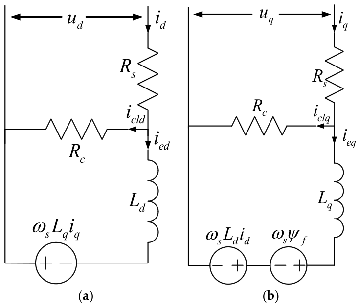
The equivalent circuit configuration of the open-winding permanent magnet synchronous motor considering iron loss in the rotor synchronous rotating reference frame is shown in Figure 2:

Here, $u_d$ and $i_d$ are the d-axis voltage and current, respectively, and $u_q$ and $i_q$ are the q-axis voltage and current, respectively. $i_d$ can be decomposed into the d-axis effective current component $i_{ed}$ and the iron loss component $i_{cld}$. Correspondingly, $i_q$ can be decomposed into the q-axis effective current component $i_{eq}$ and the iron loss component $i_{clq}$. $R_s$ and $R_c$ are the stator armature resistance and equivalent iron loss resistance of the motor, respectively. $L_d$ and $L_q$ are the d-axis and q-axis inductances. ${\omega }_s$ is the rotor electrical angular velocity. ${\psi }_f$ is the permanent magnet flux linkage.

Based on the equivalent circuit configuration shown in Figure 2, the equivalent voltage equations of the OW-PMSM in the rotor synchronous reference frame can be derived:

$$\left\{\begin{array}{l}{u}_d=R_s{i}_{ed}+K_c(L_d{\displaystyle \frac{d{i}_{ed}}{dt}}-{\omega }_s{L}_q{i}_{eq})\\ u_q=R_s{i}_{eq}+K_c\left[L_q{\displaystyle \frac{d{i}_{eq}}{dt}}+{\omega }_s(L_d{i}_{ed}+{\psi }_f)\right]\end{array}\right.$$

(1)

Here, $K_c={\displaystyle \frac{R_s}{R_c}}+1$ represents the influence of iron loss on the motor.

The expression for electromagnetic torque is:

$$T_e=p_0{i}_{eq}[{\psi }_f+(L_d-L_q)i_{ed}]$$

(2)

where $p_0$ is the number of pole pairs. Since we adopt a power-invariant transformation, the electromagnetic torque formula does not include the coefficient ${\displaystyle \frac{3}{2}}$.

2.2. Power Allocation Mechanism and Feasible Region Derivation

The dual-inverter OW-PMSM drive system with isolated DC buses is shown in Figure 1. The power sources of the drive system comprise a primary energy source and a secondary energy source, with $U_{dc1}$ and $U_{dc2}$ representing their respective DC bus voltages. The output voltages of Inverter I, taking point $O_1$ as reference, are $u_{X{O}_1},u_{Y{O}_1},u_{Z{O}_1}$, respectively. The output voltages of Inverter II, taking point $O_2$ as reference, are $u_{U{O}_2},u_{V{O}_2},u_{W{O}_2}$, respectively. The motor three-phase winding voltages $u_{XU},u_{YV},u_{ZW}$ and the inverter output voltages satisfy Kirchhoff’s voltage law:

$$\left\{\begin{array}{c}{u}_{UX}=u_{U{O}_1}-u_{X{O}_2}+u_{O_1{O}_2}\\ u_{VY}=u_{V{O}_1}-u_{Y{O}_2}+u_{O_1{O}_2}\\ u_{WZ}=u_{W{O}_1}-u_{Z{O}_2}+u_{O_1{O}_2}\end{array}\right.$$

(3)

where $u_{O_1{O}_2}$ is the potential difference between the midpoints of the two power sources.

In the stator phase plane of the motor, the stator voltage vector $\overrightarrow{u_s}$ can be synthesized from the motor phase voltages:

$$\overrightarrow{u_s}=\sqrt{{\displaystyle \frac{2}{3}}}(u_{UX}{e}^{j0}+u_{VY}{e}^{j{\displaystyle \frac{2\pi }{3}}}+u_{WZ}{e}^{j{\displaystyle \frac{4\pi }{3}}})$$

(4)

where $e^{j0}$, $e^{j{\displaystyle \frac{2\pi }{3}}}$, and $e^{j{\displaystyle \frac{4\pi }{3}}}$ are the spatial operators, and $\sqrt{{\displaystyle \frac{2}{3}}}$ is the equal-power transformation factor.

If $\overrightarrow{u_{pi}}$ and $\overrightarrow{u_{si}}$ represent the voltage vectors output by the primary inverter and the secondary inverter, respectively, Equation (4) can be expressed as:

$$\left\{\begin{array}{l}\overrightarrow{u_{pi}}=\sqrt{{\displaystyle \frac{2}{3}}}(u_{X{O}_1}{e}^{j0}+u_{Y{O}_1}{e}^{j{\displaystyle \frac{2\pi }{3}}}+u_{Z{O}_1}{e}^{j{\displaystyle \frac{4\pi }{3}}})\\ \overrightarrow{u_{si}}=\sqrt{{\displaystyle \frac{2}{3}}}(u_{U{O}_2}{e}^{j0}+u_{V{O}_2}{e}^{j{\displaystyle \frac{2\pi }{3}}}+u_{W{O}_2}{e}^{j{\displaystyle \frac{4\pi }{3}}})\end{array}\right.$$

(5)

Further, the expression for $\overrightarrow{u_s}$ can be obtained:

$$\overrightarrow{u_s}=\overrightarrow{u_{pi}}-\overrightarrow{u_{si}}+\sqrt{{\displaystyle \frac{2}{3}}}{u}_{O_1{O}_2}(e^{j0}+e^{j{\displaystyle \frac{2\pi }{3}}}+e^{j{\displaystyle \frac{4\pi }{3}}})=\overrightarrow{u_{pi}}-\overrightarrow{u_{si}}$$

(6)

Similarly, the stator current vector $\overrightarrow{i_s}$ can be synthesized from the currents in the three-phase windings of the motor:

$$\overrightarrow{i_s}=\sqrt{{\displaystyle \frac{2}{3}}}(i_U{e}^{j0}+i_V{e}^{j{\displaystyle \frac{2\pi }{3}}}+i_W{e}^{j{\displaystyle \frac{4\pi }{3}}})$$

(7)

From Equation (7), it can be seen that the stator voltage vector $\overrightarrow{u_s}$ can be expressed as the vector difference in the output voltage vectors of the dual inverters and is independent of the potential difference between the midpoints of the two DC power sources. This characteristic provides a theoretical foundation for the voltage modulation and coordinated control of the dual inverters.

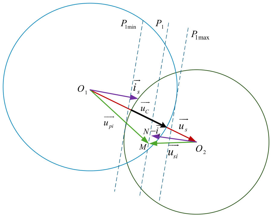
Figure 3 illustrates the voltage vector synthesis and power allocation mechanism. The feasible range of power allocation for dual inverters is constrained by their respective voltage modulation capabilities. Taking the reference point $O_1$ of Inverter I as the center and $\sqrt{1/2}{U}_{dc1}$ as the radius, circle $O_1$ is drawn, representing the voltage modulation range of Inverter I. Correspondingly, taking the reference point $O_2$ of Inverter II as the center and $\sqrt{1/2}{U}_{dc2}$ as the radius, circle $O_2$ is drawn, representing the voltage modulation range of Inverter II. According to Equation (6), the endpoint of the voltage vector of Inverter I and the endpoint of the voltage vector of Inverter II must coincide at the same point $M$. The intersection of the two circles constitutes the feasible region for voltage vector allocation. Only when point $M$ lies within this feasible region can the voltages of both inverters be fully modulated simultaneously. Quantitatively, an increase in either $U_{dc1}$ or $U_{dc2}$ enlarges the corresponding circle and shifts the position of their intersection. Consequently, the area and shape of this feasible region vary with changes in the individual DC bus voltages, directly influencing the boundary of the linear power allocation range.

In the figure, $P_1$ is the output power of Inverter I, $P_2$ is the output power of Inverter II, and $P_s$ is the input power at the motor terminals. These three can be expressed as:

$$\left\{\begin{array}{l}{P}_1=\overrightarrow{u_{mi}}\cdot \overrightarrow{i_s}\\ P_2=\overrightarrow{u_{si}}(-\overrightarrow{i_s})=-\overrightarrow{u_s}\cdot \overrightarrow{i_s}\\ P_s=\overrightarrow{u_s}\cdot \overrightarrow{i_s}\end{array}\right.$$

(8)

And they are satisfied:

$$P_s=P_1+P_2$$

(9)

$P_1$ and $P_2$ are positive when the inverters are outputting power and negative when they are absorbing power.

The intersection of the two voltage circles represents the ideal power allocation range for the dual inverters. $\overrightarrow{u_C}$ is the component of $\overrightarrow{u_s}$ lying in the overlapping part of the two circles, representing the linear voltage vector allocation range of the two inverters. Taking point $M$ as an example, the allocated power at this point can be expressed as the vector product (dot product) of the voltage $\overrightarrow{u_{pi}}$ and the current $\overrightarrow{i_s}$, which is the power represented by $P_1$. When point $M$ moves along the line $P_1$, the power represented remains constant. The dashed line representing $P_1$ is perpendicular to $\overrightarrow{i_s}$, the dashed line for $P_1$ translates left or right accordingly. Furthermore, when $\overrightarrow{u_{pi}}$ is located at the edge of the two voltage circles, the allocated power reaches its maximum value $P_{1\max }$ or minimum value $P_{1\min }$.

2.3. Analysis of Voltage and Current Vector Operating Limits

During actual motor operation, it is subject to the constraints of maximum voltage and maximum current. Ignoring iron loss, Equation (1) can be simplified as follows:

$$\left\{\begin{array}{l}{u}_d=R_s{i}_d+L_d{\displaystyle \frac{d{i}_d}{dt}}-{\omega }_s{L}_q{i}_q\\ u_q=R_s{i}_q+L_q{\displaystyle \frac{d{i}_q}{dt}}+{\omega }_s(L_d{i}_d+{\psi }_f)\end{array}\right.$$

(10)

The stator current vector $\overrightarrow{i_s}$ is limited by the maximum current amplitude $i_{s\max }$:

$$\left|\overrightarrow{i_s}\right|=\sqrt{i_d^2+i_q^2}\le i_{s\max }$$

(11)

The stator voltage vector $\overrightarrow{u_s}$ is limited by the DC bus voltage and the modulation strategy. The maximum voltage amplitude $u_{s\max }$ is determined by the sum of the dual-inverter DC bus voltages:

$$\left|\overrightarrow{u_s}\right|=\sqrt{u_d^2+u_q^2}\le u_{s\max }=\sqrt{{\displaystyle \frac{1}{2}}}(U_{dc1}+U_{dc2})$$

(12)

Combining Equations (11) and (12), and neglecting the transient terms, the voltage constraint ellipse equation that $i_d$ and $i_q$ must satisfy under steady-state conditions can be obtained:

$${\displaystyle \frac{{\left(i_d+{\psi }_f/L_d\right)}^2}{1/L_d^2}}+{\displaystyle \frac{i_q^2}{1/L_q^2}}\le {\displaystyle \frac{u_{s\max }^2}{{\omega }_s^2}}={\displaystyle \frac{{\left(U_{dc1}+U_{dc2}\right)}^2}{2{\omega }_s^2}}$$

(13)

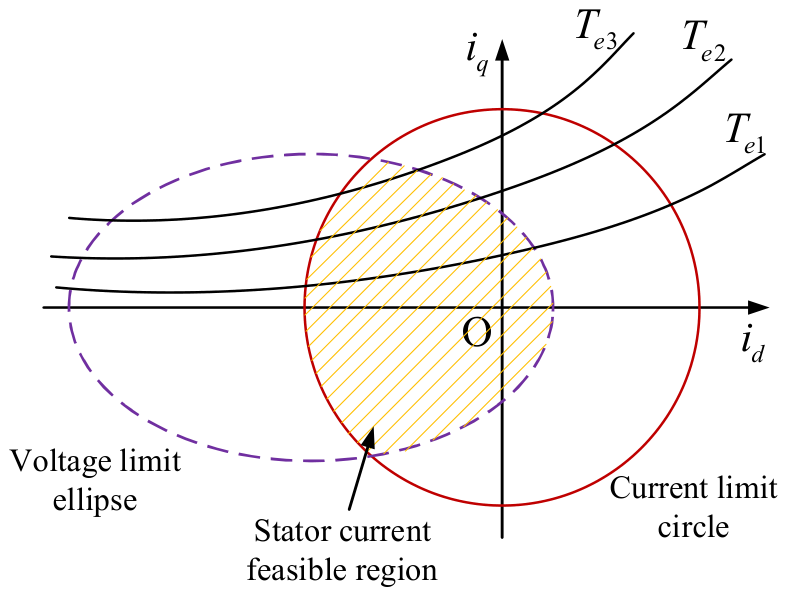
The current limit circle defined by Equation (11) and the voltage limit ellipse defined by Equation (13) together constitute the feasible steady-state operating region of the motor, as shown in Figure 4.

According to the definition of Equation (13), an increase in either $U_{dc1}$ or $U_{dc2}$ will enlarge the coverage area of the ellipse, thereby expanding the entire steady-state operating range of the current vector. The curves $T_{e1}$, $T_{e2}$, $T_{e3}$ shown in the figure indicate that the motor maintains a constant electromagnetic torque along this curve. When the motor operating point lies within the intersection region enclosed by the current limit circle and the voltage limit ellipse, the motor neither exceeds the current capacity constraint nor the voltage modulation capability constraint, and the system is well behaved and controllable.

3. Steady-State Stator Current Optimization Strategies

This subsection proposes two stator current planning algorithms, i.e., the Loss Minimization Algorithm (LMA) and the Maximum Power Allocation Range Algorithm (MPAR), aimed at minimizing the electrical losses of the motor and maximizing the power allocation range of the two inverters, respectively. Through a dynamic switching strategy between the two algorithms, the requirements for both efficiency and stability during motor operation can be balanced.

This paper focuses on the optimization and control of a vehicle-mounted OW-PMSM, and the parameters of the drive system are shown in

Table 1. Parameters of the OW-PMSM drive system.

Parameter	Value
$\mathrm{Rotor}\mathrm{pole}\mathrm{pairs}{p}_0$	4
$\mathrm{Armature}\mathrm{resistance}{R}_s/\Omega$	0.1
$\mathrm{Equivalent}\mathrm{iron}\mathrm{loss}\mathrm{resistance}{R}_c/\Omega$	90
$\mathrm{Permanent}\mathrm{magnet}\mathrm{flux}\mathrm{linkage}{\psi }_f/\mathrm{Wb}$	0.216
$\mathrm{Stator}\mathrm{inductance}\mathrm{of}\mathrm{d}\text{-}\mathrm{axis}{L}_d/\mathrm{H}$	0.73 × 10−3
$\mathrm{Stator}\mathrm{inductance}\mathrm{of}\mathrm{q}\text{-}\mathrm{axis}{L}_q/\mathrm{H}$	1.57 × 10−3
$\mathrm{Current}\mathrm{limit}\mathrm{of}\mathrm{power}\mathrm{device}{i}_{\lim }/\mathrm{A}$	280
$\mathrm{DC}1\mathrm{voltage}{U}_{dc1}/\mathrm{V}$	350
$\mathrm{DC}2\mathrm{voltage}{U}_{dc2}/\mathrm{V}$	250

.

3.1. Loss Minimization Algorithm (LMA) for Efficiency Optimization

The Loss Minimization Algorithm focuses on minimizing the resistance losses and iron losses of the motor under steady-state conditions. Based on the equivalent circuit configuration in Figure 2, the electrical losses of the motor during steady-state operation can be derived:

$$\left\{\begin{array}{l}{P}_{Re}=R_s(i_d^2+i_q^2)=R_s\{{(i_{ed}-{\displaystyle \frac{{\omega }_s{L}_q{i}_{vd}}{R_c}})}^2+{[i_{ed}+{\displaystyle \frac{{\omega }_s(L_d{i}_{ed}+{\psi }_f)}{R_c}}]}^2\}\\ P_{Fe}=R_c\cdot (i_{cld}^2+i_{clq}^2)=\left({\displaystyle \frac{{\omega }_s^2}{R_c}}\right)[{(L_d{i}_{ed}+{\psi }_f)}^2+{(L_q{i}_{eq})}^2]\end{array}\right.$$

(14)

where $P_{Re}$ is the copper loss, $P_{Fe}$ is the iron loss, and $P_T$ represents the total electrical losses.

$$P_T=P_{Re}+P_{Fe}$$

(15)

Based on this, the core formulation of the LMA for current vector planning can be derived:

$$\begin{array}{l}\min P_T(i_d,i_q)\\ s.t.\left|\overrightarrow{i_s}\right|(i_d,i_q)\le i_{s\max }\\ \left|\overrightarrow{u_s}\right|(i_d,i_q)\le u_{s\max }\end{array}$$

(16)

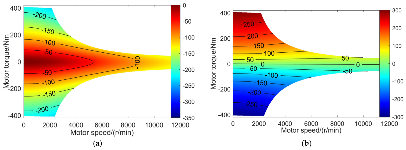
By numerically solving the problem at each motor operating point, the reference stator current vector under the LMA can be obtained. The specific procedure is as follows: an offline solution over the entire speed-torque operating envelope of the motor is carried out in MATLAB (R2020a version) using a dense grid search combined with an interior-point algorithm, ensuring reliable convergence to the global optimum at each grid point. The results of this offline optimization are stored in the motor controller as two-dimensional lookup tables, which map the input reference torque and speed to the optimal d-axis and q-axis current pairs for each algorithm. During operation, the required current references for a given operating point are obtained through fast bilinear interpolation between the pre-computed grid points. This approach improves control accuracy while minimizing the computational burden, thereby enhancing hardware adaptability. 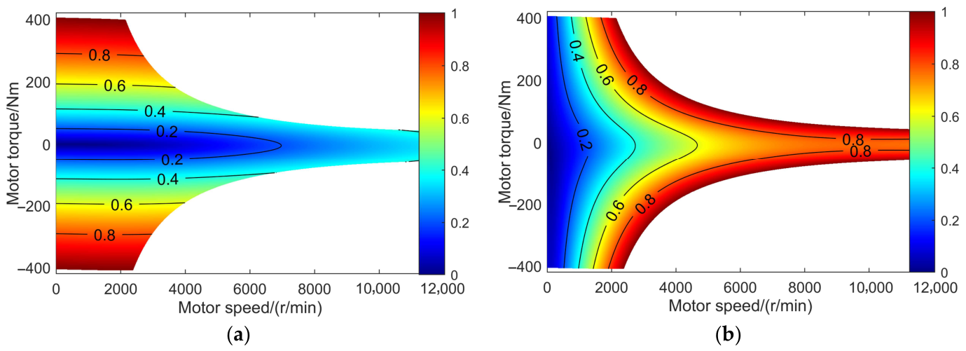After the optimization is completed, the MAPs of the stator current components over the entire motor operating range are shown in Figure 5. The saturation rates of the stator current and stator voltage are shown in Figure 6. The saturation rate indicates how close the stator current amplitude and stator voltage amplitude are to their respective maximum allowable limits. The first quadrant represents the motor operating in motoring mode, while the fourth quadrant represents the motor operating in generating mode.

The magnitude of $i_q$ is influenced by the motor speed and output torque and is proportional to the absolute value of the output torque. The magnitude of $i_d$ is also determined by the motor speed and electromagnetic torque, with the output torque having a more significant impact. Therefore, changes in motor speed have a relatively minor effect on the stator current saturation rate, while the absolute value of the output torque has the most significant impact. However, when the motor is in a low-load region, as the speed increases, the stator current amplitude increases, and the saturation rate rises accordingly. The stator voltage saturation rate is primarily affected by the motor speed. In the low-speed region, the output torque has a considerable influence on the stator voltage saturation rate. As the speed increases, its impact on the stator voltage saturation rate becomes progressively more pronounced. This characteristic causes both the stator voltage saturation rate and the stator current saturation rate to extend into the high-speed region.

3.2. Maximum Power Allocation Range Algorithm (MPAR) for Operational Flexibility

In the previously proposed Maximum Voltage Allocation Range algorithm [5], as shown in Figure 3, the magnitudes of $U_{dc1}$ and $U_{dc2}$ are determined by the DC bus voltages. Therefore, to expand the voltage allocation range, the amplitude of $\overrightarrow{u_s}$ can be minimized, thereby broadening the intersection area of the two voltage circles. However, this method fails to consider the influence of the stator current $\overrightarrow{i_s}$ on power allocation, resulting in an indirectly calculated power allocation range that cannot reach its maximum. Based on this, this paper proposes the Maximum Power Allocation Range Algorithm (MPAR), aiming to directly obtain the maximum linear power allocation.

As shown in Figure 3, $\overrightarrow{u_C}$ represents the component of $\overrightarrow{u_s}$ that lies within the feasible region for voltage vector allocation, representing the linear voltage vector allocation range of the two inverters. The core computational expression of this algorithm is as follows:

$$\begin{array}{l}{P}_{mi}=\stackrel{\rightharpoonup }{u_C}\cdot \stackrel{\rightharpoonup }{i_s}=u_{Cd}{i}_d+u_{Cq}{i}_q\\ ={\displaystyle \frac{\left(u_{s\max }-u_{s\_amp}\right)}{u_{s\_amp}}}{u}_d{i}_d+{\displaystyle \frac{\left(u_{s\max }-u_{s\_amp}\right)}{u_{s\_amp}}}{u}_q{i}_q\\ ={\displaystyle \frac{u_{s\max }-u_{s-amp}}{u_{s\_amp}}}\left(u_d{i}_d+u_q{i}_q\right)\end{array}$$

(17)

In the formula, $P_{mi}$ is the maximum linear power allocation, $u_{s\max }=\sqrt{1/2}(U_{dc1}+U_{dc2})$ represents the sum of the maximum amplitudes of the two voltage vectors, and $u_{s\_amp}$ is the amplitude of the stator voltage vector. By expressing $P_{mi}$ as the vector product of $\overrightarrow{u_C}$ and $\overrightarrow{i_s}$, the angle factor between them can be considered. Therefore, the MPAR can also be simplified to a problem of maximizing a single-variable function under inequality constraints.

Based on this, the core formulation of the MPAR for current vector planning can be similarly derived:

$$\begin{array}{l}\max P_C(i_d,i_q)\\ s.t.\left|\overrightarrow{i_s}\right|(i_d,i_q)\le i_{s\max }\\ \left|\overrightarrow{u_s}\right|(i_d,i_q)\le u_{s\max }\end{array}$$

(18)

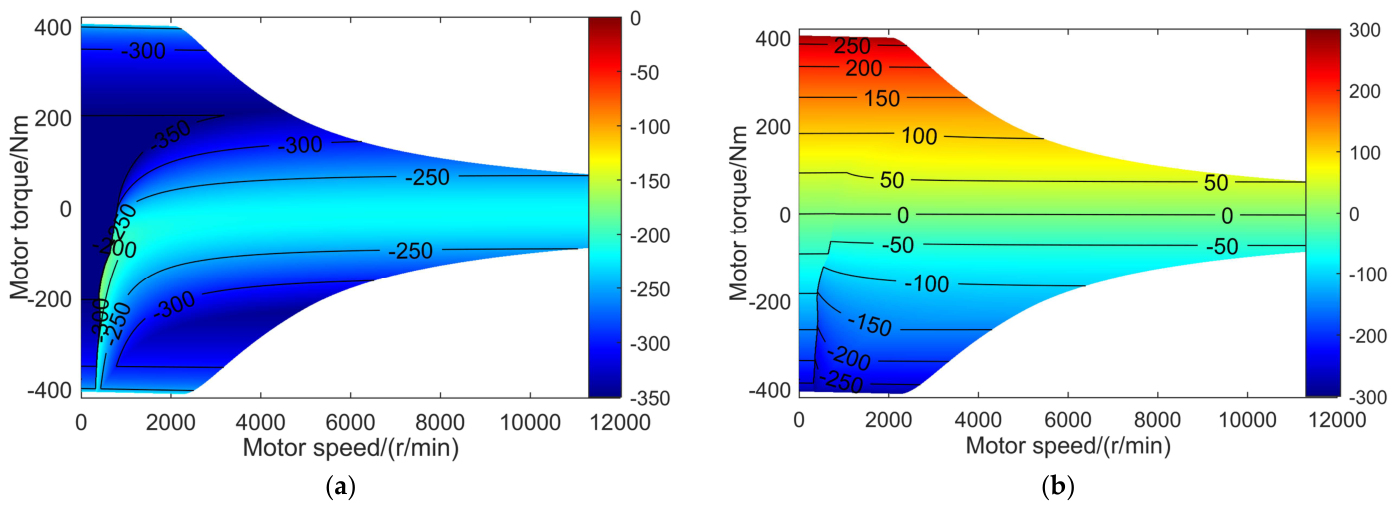
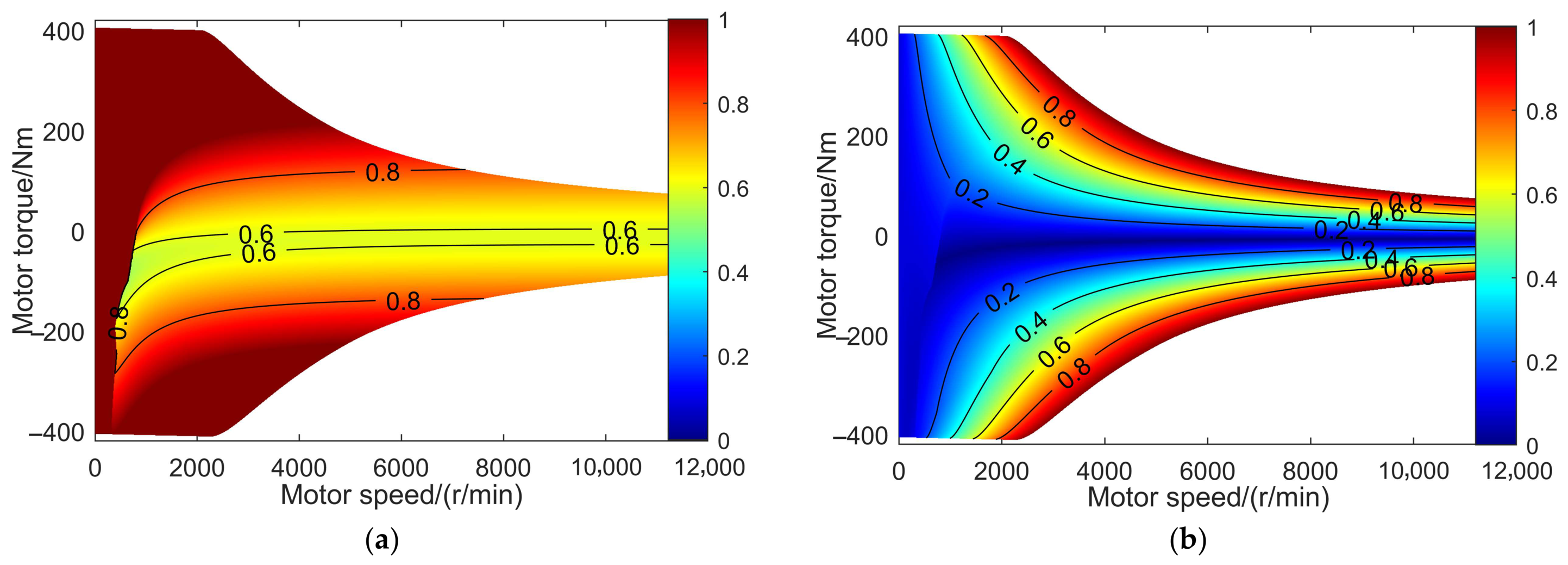
After obtaining the core formulation of the MPAR, the solving process in Section 3.1 is repeated to obtain the reference stator current vector under the MPAR. After the optimization is completed, the MAPs of the stator current components over the entire operating range of the motor are shown in Figure 7. The saturation rates of the stator current and stator voltage are shown in Figure 8.

From the figures, it can be observed that in the medium-to-high-speed range, the magnitude of $i_d$ is primarily affected by the absolute value of the torque and is less influenced by the speed. However, when the motor speed is low, the magnitude of $i_d$ is generally larger and not significantly affected by torque variations. The magnitude of $i_q$ is relatively evenly distributed throughout the motor’s operating range and is proportional to the torque. Compared with the LMA, at the same motor speed, the MPAR provides a larger d-axis current, while its stator current saturation rate is significantly higher than that of the LMA. This characteristic allows the motor’s characteristic region to expand in both the motoring and generating regions at medium and high speeds.

3.3. Comparative Analysis of Steady-State Performance

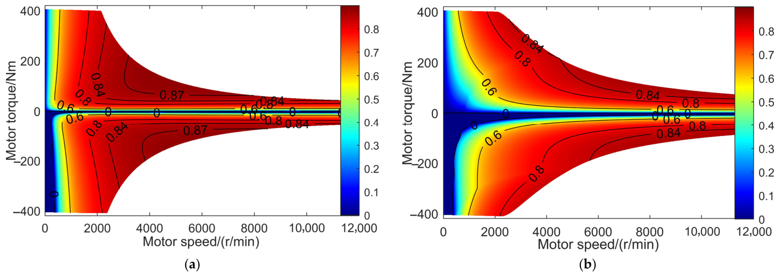
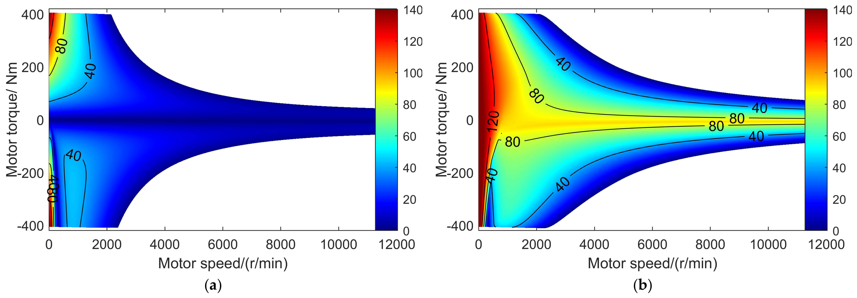
The differences between the two proposed algorithms in terms of steady-state efficiency and linear power allocation range are shown in Figure 9 and Figure 10, respectively. In Figure 10, the unit of power is kW.

From the comparison in Figure 9, it can be concluded that, at the same motor operating point, the efficiency of the LMA is significantly better than that of the MPAR. However, the efficiency of the MPAR improves when it approaches the boundary region of its characteristic range. In Figure 10, the LMA clearly lacks the capability for power allocation optimization during light-load conditions and in the medium-to-high-speed range. Based on the above analysis, the motor can be operated within the region defined by the LMA by default to minimize electrical losses during operation. When the motor operating point exceeds the limits of the LMA, the system automatically switches to the MPAR, thereby enhancing the system’s linear power allocation capability. Meanwhile, to prevent rapid, undesirable chattering between the two algorithms near the boundary of the LMA region, the switching strategy implements a switching frequency limitation.

In practice, the LMA should be used as the default strategy for general operation to maximize system efficiency and minimize electrical losses. The MPAR should be activated when the drive system requires either an expanded steady-state operational envelope or a maximized power allocation range between the dual energy sources. Specifically, it is employed during high dynamic demands, aggressive driving cycles, or when the requested operating point falls outside the feasible region of the LMA. This strategy extends the system’s external characteristic limits, allowing operation at higher torque or wider speed ranges, while prioritizing and enhancing the capability for flexible power transfer between the two isolated sources.

4. Coordinated Control of Electromagnetic Torque and d-Axis Current

The LMA and MPAR primarily focus on minimizing motor losses and maximizing the power allocation range in steady state, respectively. During actual operation, the motor selects the corresponding stator current planning algorithm based on the requirements of the specific operating conditions. To minimize efficiency losses during motor operation, the LMA is preferentially used within its allowable power allocation range. When power allocation demand from the energy management module exceeds the power allocation range of the LMA, the system switches to the MPAR. The transition between the two algorithms is often accompanied by transient current fluctuations. To address such issues, the current mainstream solution is the decoupled PI control scheme. For instance, the improved current decoupling method based on active disturbance rejection control proposed in Reference [19] is essentially still dq-axis current decoupling control. However, with this method, the torque tracking performance and the stability during motor operation cannot be effectively ensured. Reference [6] proposed a composite sliding mode control algorithm, using d-axis current and torque as sliding surfaces, which reduces the electromagnetic torque ripple during motor operation. However, its computational process is relatively complex, and instability in the electromagnetic torque and rotor speed may occur due to the current amplitude exceeding the optimal current range, thus failing to effectively guarantee stability. Therefore, this paper directly uses voltage vector allocation based on the reference d-axis current and torque values, achieving a smooth transition for the motor between the two stator current planning algorithms.

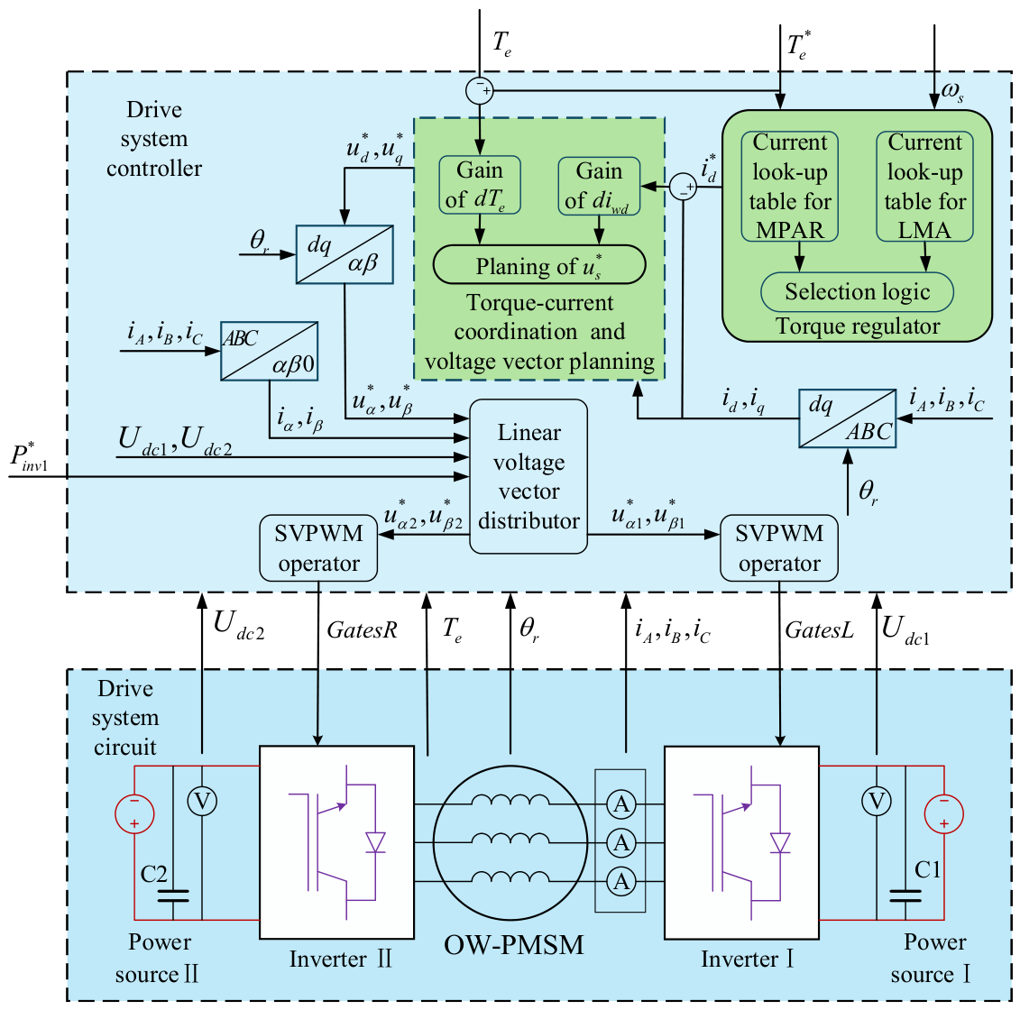
The overall control framework is shown in Figure 11:

In the torque regulator module, the desired dq-axis currents under the current operating conditions are computed based on the input reference electromagnetic torque. These desired currents, together with the reference torque, are fed as inputs to the torque–current coordination and voltage vector planning module, which, in combination with the current electromagnetic torque output by the motor, generates the corresponding reference voltage vector. In the linear voltage vector distribution module, the voltage vector is allocated according to the motor’s present operating parameters, and the resulting voltages are then input to the dual space vector pulse width modulation (SVPWM) modules.

4.1. Basic Principle of the Coordination Strategy

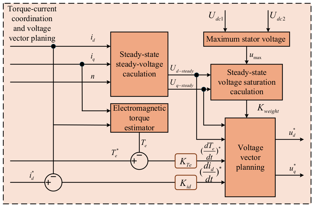
The coordinated control of electromagnetic torque and d-axis current aims to ensure the tracking performance of the d-axis current and motor torque during operation with minimal computational effort. The previously mentioned LMA and MPAR calculate the expected dq-axis currents $i_d^{*}$ and $i_q^{*}$, as well as the expected electromagnetic torque $T_e^{*}$, for the motor’s next operating instant. By comparing these with the motor’s current operating parameters, the required d-axis current adjustment $\Delta i_d$ and electromagnetic torque adjustment $\Delta T_e$ for the current instant can be obtained. They need to be multiplied by their corresponding gain coefficients, $K_{Te}$ and $K_i^d$. The resulting dq-axis voltage gains are then combined with the current stator voltage to obtain the expected dq-axis voltages $u_d^{*}$ and $u_q^{*}$ for the motor at the next instant. The control framework is shown in Figure 12:

In the figure, $U_{d-steady}$ and $U_{q-steady}$ represent the dq-axis voltages under the current steady-state condition, which can be calculated using the following equations:

$$\left\{\begin{array}{l}{U}_{d-steady}=R_s{i}_d-K_c{L}_q{i}_q{\omega }_s\\ U_{q-steady}=R_s{i}_q+K_c{\omega }_s(L_d{i}_q+{\psi }_f)\end{array}\right.$$

(19)

Under steady-state conditions, the voltage requirements arising from the rate of change of $i_d$ and $T_e$ are further calculated. First, the expected rate of change in the d-axis current ${({\displaystyle \frac{d{i}_d}{dt}})}^{*}$ and the expected rate of change in the electromagnetic torque ${({\displaystyle \frac{d{T}_e}{dt}})}^{*}$ are computed using the following formulas:

$$\left\{\begin{array}{l}{({\displaystyle \frac{d{T}_e}{dt}})}^{*}=K_{Te}(T_e^{*}-T_e)\\ {({\displaystyle \frac{d{i}_d}{dt}})}^{*}=K_{id}(i_d^{*}-i_d)\end{array}\right.$$

(20)

where $K_{Te}$ is the electromagnetic torque gain coefficient, and $K_i^d$ is the d-axis current gain coefficient. These two parameters can be adjusted according to the corresponding deviations of the electromagnetic torque and d-axis current.

After all the above parameters are calculated, the unconstrained expected dq-axis output voltages $u_{uld}^{*}$ and $u_{ulq}^{*}$ of the motor can be obtained through voltage vector planning. The calculation method is as follows:

$$\left\{\begin{array}{l}{u}_{uld}^{*}=K_c{L}_d{({\displaystyle \frac{d{i}_d}{dt}})}^{*}+U_{d-steady}\\ u_{ulq}^{*}={\displaystyle \frac{K_c{L}_q}{p_0[{\psi }_f+i_d(L_d-L_q)]}}{({\displaystyle \frac{d{T}_e}{dt}})}^{*}+U_{q-steady}\end{array}\right.$$

(21)

4.2. Feasible Region Analysis and Dynamic Voltage Vector Planning

When $u_{uld}^{*}$ and $u_{ulq}^{*}$ lie within the constraint range of $u_{s\max }$, they can be directly used as the expected dq-axis output voltages. However, when $u_{uld}^{*}$ and $u_{ulq}^{*}$ exceed the constraint range of $u_{s\max }$, the voltage vector should be selected within the feasible region limited by $u_{s\max }$, choosing the maximum voltage amplitude possible while remaining as close as possible to $u_{uld}^{*}$ and $u_{ulq}^{*}$. 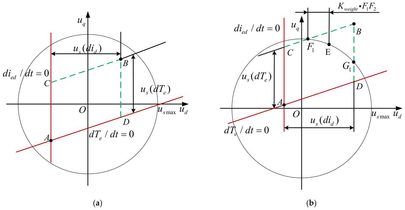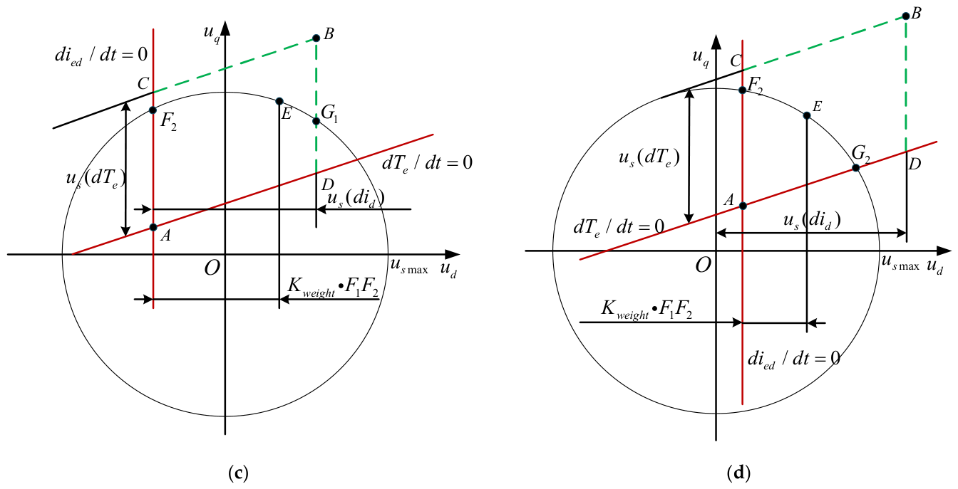Based on this, a parallelogram-based voltage vector allocation algorithm is constructed, as shown in Figure 13. Point A represents the steady-state voltage that maintains the current operating point of the motor. Point B represents the coordinate point constituted by $u_{uld}^{*}$ and $u_{ulq}^{*}$. Point D is the coordinate point that satisfies only the ${({\displaystyle \frac{d{i}_d}{dt}})}^{*}$ requirement. Point C is the voltage vector coordinate point that satisfies only the ${({\displaystyle \frac{d{T}_e}{dt}})}^{*}$ requirement.

In the figure, $u_s(d{i}_d)$ and $u_s(d{T}_e)$ represent the desired voltage gains for the d-axis current and the electromagnetic torque, respectively. When point B lies within the constraint range of $u_{s\max }$, point B can be directly selected as the desired dq-axis output voltages $u_d^{*}$ and $u_q^{*}$, denoted as case 1, shown in Figure 13a.

When point B exceeds the constraint range of $u_{s\max }$, the situation needs to be discussed case by case. Let $F_1$, $F_2$, $G_1$ and $G_2$ be the intersection points of lines BC, AC, BD and AD with the voltage limit circle, respectively. Accordingly, cases 2–4 can be distinguished, as shown in Figure 13b–d). They represent, respectively, the situation where the full required gains for both $T_e$ and $i_{ed}$ can be satisfied; the situation where only the full required gain for one of them can be satisfied (taking the case where the full required gain for $i_{ed}$ is satisfied as an example); and the situation where neither of the required gains can be fully satisfied. On this basis, both $F_1$ and $F_2$ are denoted as point $F$, and both $G_1$ and $G_2$ are denoted as point $G$. Therefore, point $E$ needs to be selected on $\stackrel{⏜}{FG}$ as the desired output voltage. For calculating the coordinates of point E, a weight factor $K_{weight}$ is introduced, which is calculated as follows:

$$K_{weight}=0.7(U_{d-steady}^2+U_{q-steady}^2)/u_{s\max }^2+0.3$$

(22)

$K_{weight}$ represents the degree of saturation of the stator voltage amplitude relative to $u_{s\max }$. When the amplitude of $u_s$ is small, to ensure current stability, a lower limit of 0.3 should be set for it to prevent the output current from dropping to zero. When the amplitude of $u_s$ approaches saturation and cannot simultaneously meet the regulation requirements of both $T_e$ and $i_{ed}$ (i.e., when $K_{weight}=1$), since the switching between the two proposed stator current planning algorithms is achieved by adjusting $i_d$, priority must be given to ensuring the regulation requirement of $i_d$. This ensures that the steady-state current conforms to the requirements of the stator current algorithm, thereby ensuring that the steady-state torque meets the demand. Considering this, the d-axis voltage at point E can be calculated as follows:

$$u_{Ed}=K_{weight}(u_{Gd}-u_{Fd})+u_{Fd}$$

(23)

$u_{Gd}$ and $u_{Fd}$ represent the d-axis voltages at points $G$ and $F$. After solving for the d-axis voltage at point E, the q-axis voltage at point E can be obtained by substituting into the analytical expression for the voltage limit circle $u_{s\max }$. Through the above method, it can be guaranteed that the expected output voltage vector of the motor during operation always remains within the limits defined by $u_{s\max }$, thus avoiding situations where point A exceeds the constraint range of $u_{s\max }$.

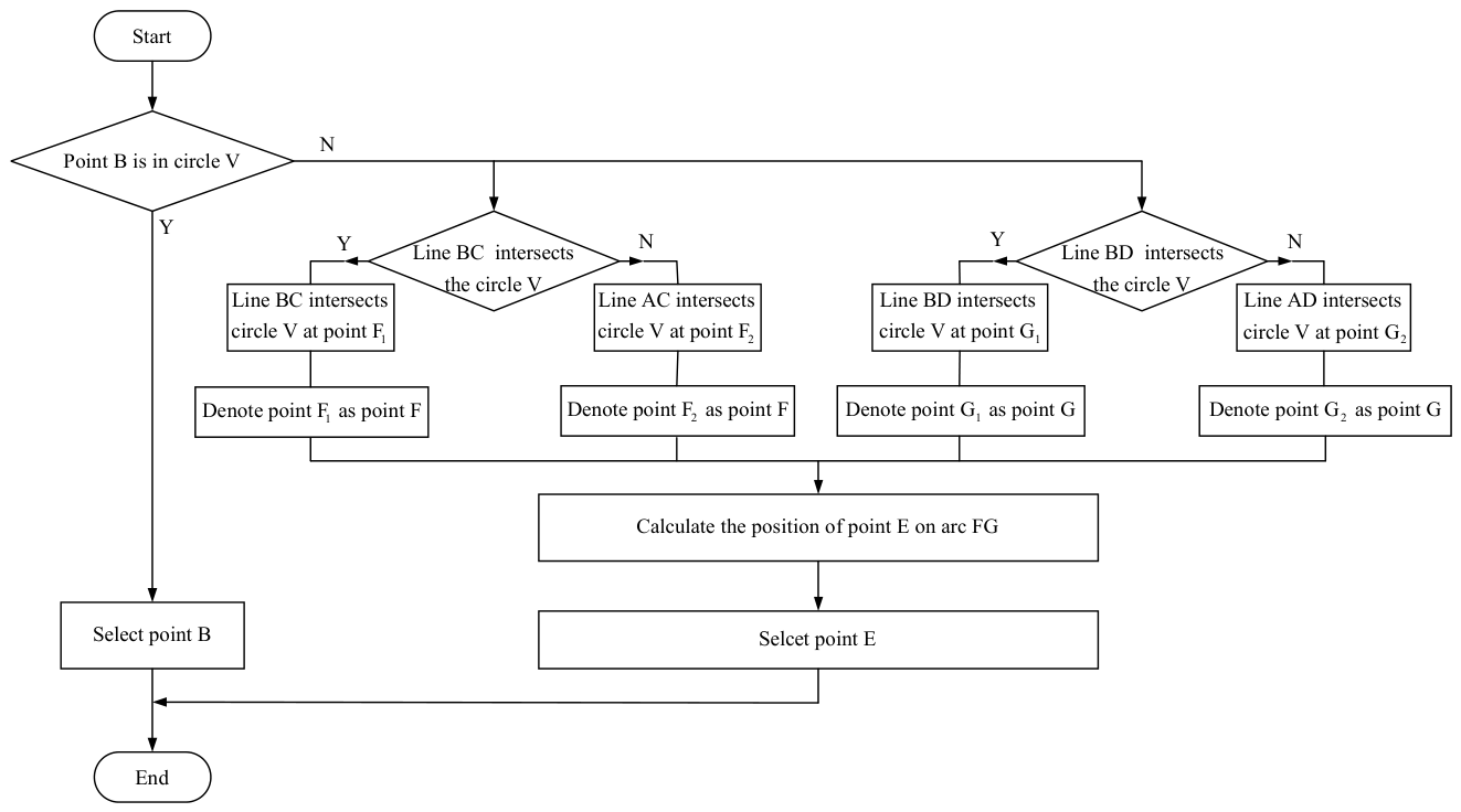
In summary, the process for solving the motor’s expected output voltage using the voltage vector allocation algorithm proposed in this paper is shown in Figure 14.

$K_{weight}$ directly reflects the instantaneous saturation level of the stator voltage relative to its maximum limit. When the voltage is not saturated, the controller has sufficient headroom to regulate both torque and d-axis current simultaneously. When the voltage approaches saturation ($K_{weight}\to 1$), the ability to satisfy both demands diminishes. The proposed algorithm uses $K_{weight}$ to explicitly prioritize the tracking of $i_{ed}$ under such saturated conditions. This approach ensures that the stator current vector follows the reference trajectory from the steady-state optimizers (LMA/MPAR), preventing current instability that could arise if the current vector falls outside the algorithm’s optimized region. Therefore, when the voltage amplitude approaches saturation, to guarantee the regulation effectiveness of $i_{ed}$, a portion of the regulation capability for $T_e$ should be sacrificed to ensure the stability of the stator current vector control. This mode defines a built-in and clear stability rule for the system: under voltage saturation conditions, priority is given to tracking the d-axis current. This rule ensures that the motor operating point never exceeds the maximum power allocation range limited by the MPAR, thereby improving the efficiency and stability of system operation. Consequently, it avoids the instability that may occur in the previous SMC method when control objectives conflict under voltage limitations. Traditional model predictive control (MPC) algorithms require evaluating multiple candidate voltage vectors or solving online optimization problems, which imposes a heavy computational burden on the control system [20]. In contrast, the proposed geometry-based voltage vector allocation scheme directly determines the optimal voltage vector through simple geometric relationships and a lightweight interpolation rule within a predefined parallelogram region. Under the premise of optimizing dynamic performance, it greatly reduces the computational load, shortens the control period, and enhances hardware adaptability.

5. Simulation and Experimental Validation

5.1. Simulation Setup and Benchmark Comparison

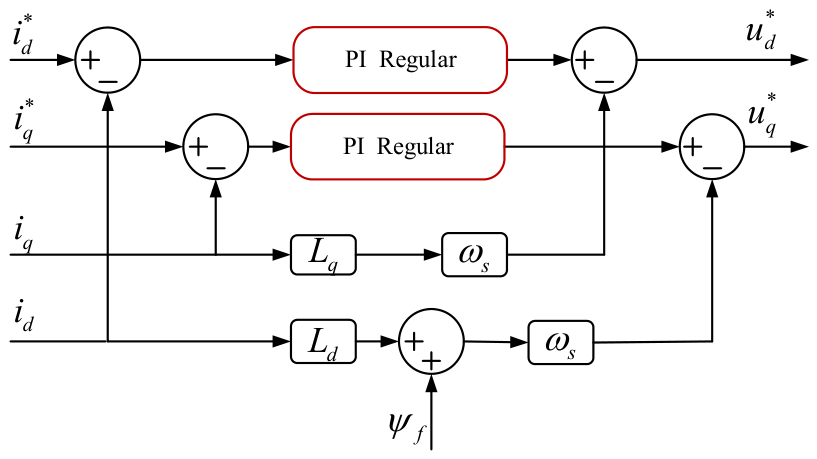
To verify the feasibility of the algorithm proposed above, decoupled PI control is used as a benchmark to compare the tracking and tracking performance of various parameters under the two algorithm modes. The mathematical formulation on which the decoupled PI control is based is as follows:

$$\left\{\begin{array}{l}{u}_d^{*}=(i_d^{*}-i_d)(K_P+K_I/p)-{\omega }_s{L}_q{i}_q\\ u_q^{*}=(i_q^{*}-i_q)(K_P+K_I/p)+{\omega }_s(L_d{i}_d+{\psi }_f)\end{array}\right.$$

(24)

where $K_P$ and $K_I$ are the proportional and integral coefficients of the system, respectively, and $p$ is the time derivative operator. Its control configuration is shown in Figure 15:

In this comparative test, both the proposed method and the decoupled PI control use the parameters provided in Table 1, with the remaining parameters listed in

Table 2. Controller parameters of the proposed method and decoupled PI control for simulation.

Controller	Parameters	Value
Proposed method	$\mathrm{Breakpoint}\mathrm{array}\mathrm{of}{K}_{Te}$	[0, 0.8, 2, 3, 5, 10, 20]
	$\mathrm{Data}\mathrm{of}{K}_{Te}$	[0, 1200, 3000, 5000, 7500, 9300, 10,500]
	$\mathrm{d}\text{-}\mathrm{axis}\mathrm{current}\mathrm{gain}\mathrm{coefficient}{K}_{id}$	1800
Decoupled PI control	$\mathrm{Proportion}\mathrm{coefficient}{K}_P$	2.5
	$\mathrm{Integration}\mathrm{coefficient}{K}_I$	100
Common Parameters	$\mathrm{Sampling}\mathrm{period}/\mathrm{ms}$	0.1
	$\mathrm{Control}\mathrm{period}/\mathrm{ms}$	0.1
	$\mathrm{SVPWM}\mathrm{frequency}/\mathrm{ms}$	10

.

For the experimental group, based on the simulation tuning results, the dynamics of the d-axis current loop are predominantly governed by the stator inductance and are consistent; therefore, a single fixed $K_{id}$ can be used to obtain satisfactory performance across the speed range. Through multiple experiments, it was found that $K_{id}=1800$ satisfies the system control performance requirements. In contrast, the dynamics of electromagnetic torque are significantly influenced by motor speed and flux linkage, making a fixed gain insufficient. Consequently, $K_{Te}$ is implemented as a speed-dependent variable, obtained by linear interpolation from a predefined lookup table. This lookup table is populated through a simulation-based system tuning process over the entire operating range to optimize the transient response during torque steps and algorithm switching, thereby ensuring stability. Accordingly, the electromagnetic torque gain coefficient $K_{Te}$ is obtained by linear interpolation from the lookup table such as Table 2.

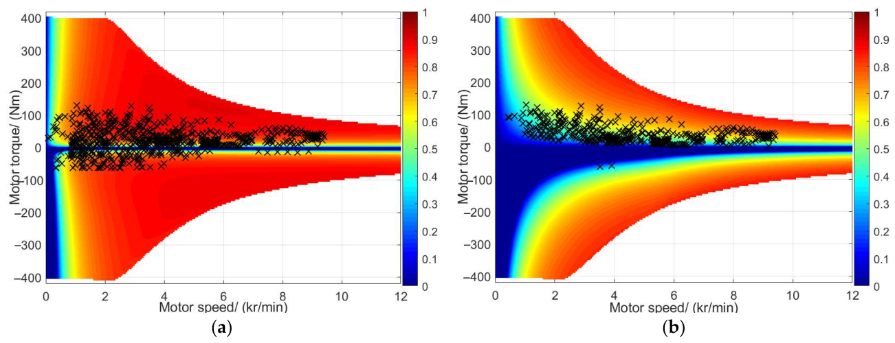
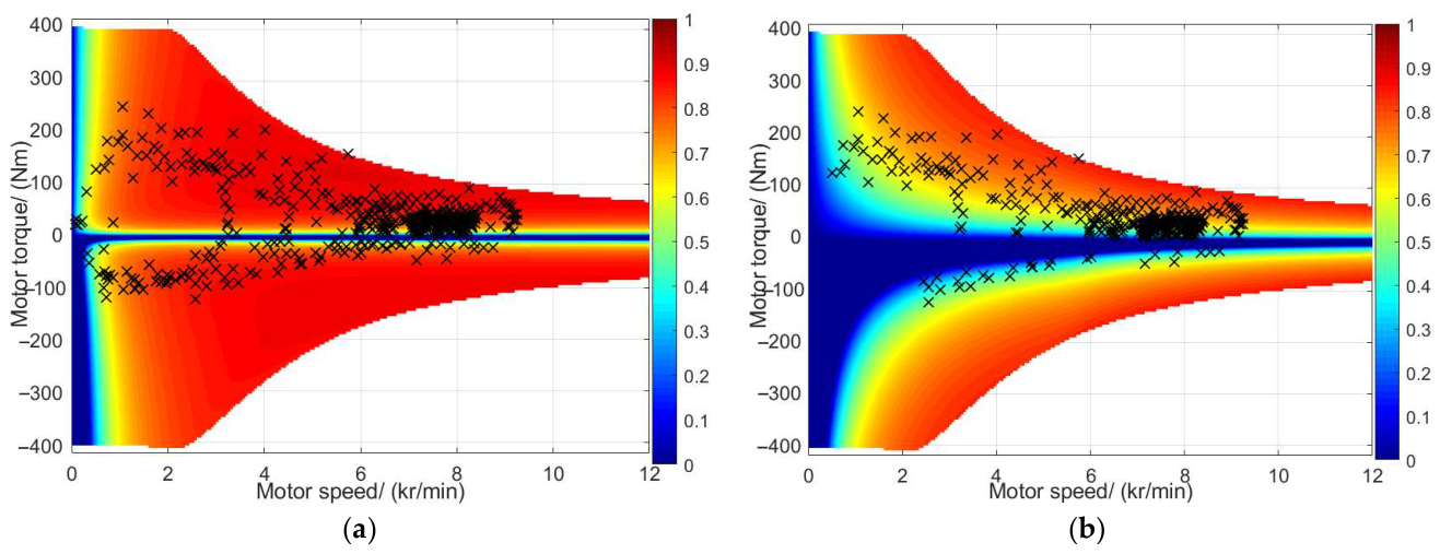
Additionally, the stator current planning algorithms employed in both groups adopt an automatic switching mode. When the motor operating state falls within the working range defined by the LMA, the LMA is preferentially selected to ensure the motor’s operational efficiency. If the operating state exceeds the range defined by the LMA, the system will automatically switch to the MPAR. The scatter plots of the motor operating points obtained under the WLTC and US06 standard driving cycles for the two algorithms are shown in Figure 16 and Figure 17, respectively. They clearly show that during the WLTC, most operating points fall within the high-efficiency region of the LMA, highlighting its primary role in improving overall energy economy. In contrast, the US06 cycle accesses operating points that frequently extend into the expanded operational region enabled by the MPAR, underscoring its critical role in providing the necessary power allocation capability during high-demand, dynamic driving.

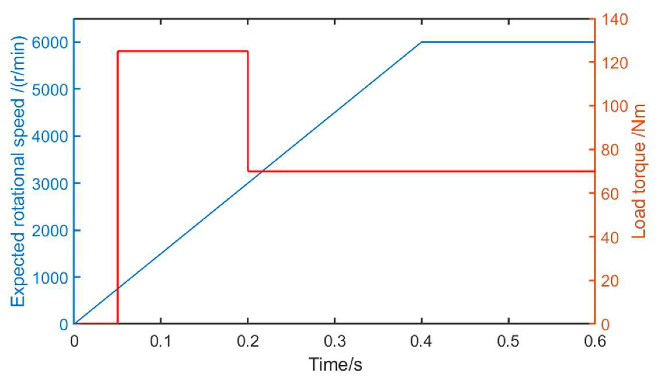
The simulation operating conditions for the experimental group and the control group are shown in Figure 18. The motor speed accelerates from 0 r/min to 6000 r/min within 0~0.4 s and then remains constant until the end. The load torque steps from 0 Nm to 120 Nm at 0.05 s, remains constant for 0.15 s, and then decreases to 70 Nm at 0.2 s, remaining constant until the end. Simulations are performed for the experimental group and the control group under these operating conditions.

5.2. Simulation Results and Analysis

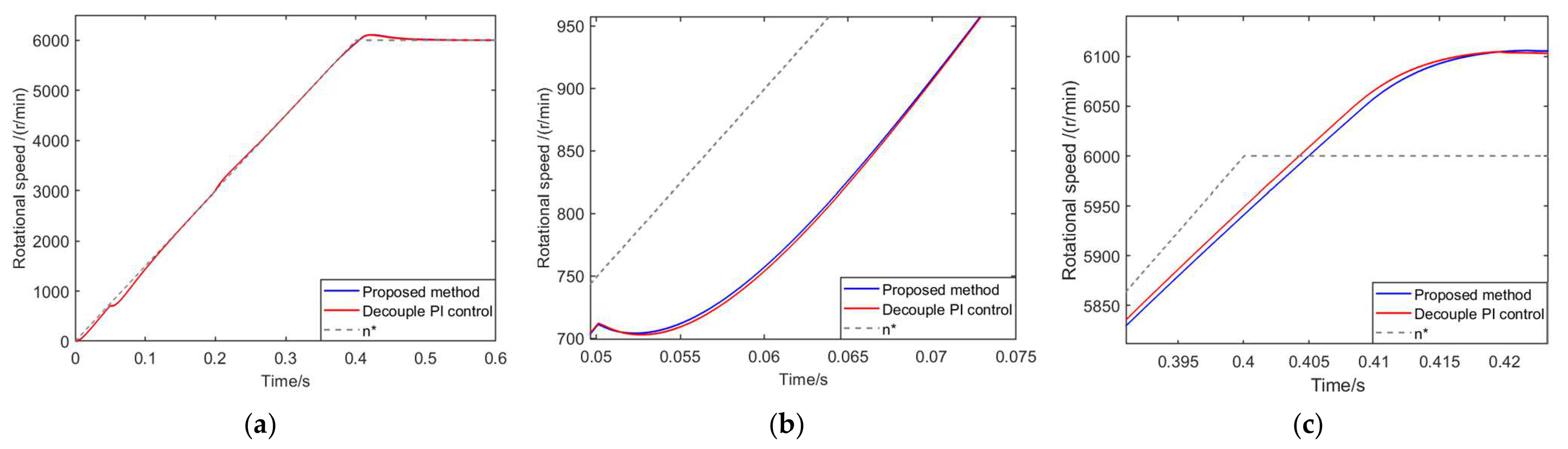
The simulation results of the proposed method and the decoupled PI control under the operating conditions shown in Figure 18 are listed as follows.

Figure 19 shows the speed tracking performance of both groups throughout the process, where $n^{*}$ represents the expected motor speed. At 0.05 s, the motor speed deviates due to the sudden change in load torque, and the deviation generated by the proposed method during this process is smaller than that of the decoupled PI control. At 0.4 s, a deviation occurs due to the change in motor speed, and the deviation generated by the proposed method during this process is also smaller than that of the decoupled PI control. Therefore, the tracking performance of the motor speed using the scheme proposed in this paper is superior to that of the traditional decoupled PI control.

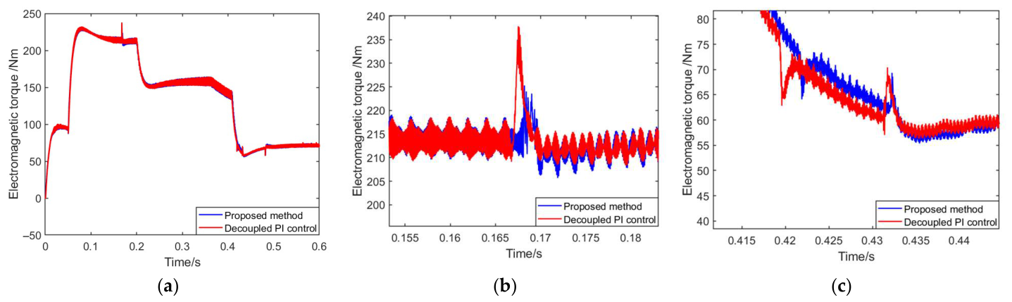
The comparison of motor torque during operation is shown in Figure 20. Within the interval of 0.165~0.170 s, a torque transient occurs due to the motor switching between the two stator current planning algorithms. At this point, the maximum overshoot of the proposed method is significantly smaller than that of the decoupled PI control, and the recovery time is shorter, indicating that the proposed method can more effectively suppress torque fluctuations during mode switching and achieve a smooth transition. Within the interval of 0.415~0.435 s, the motor experiences two consecutive algorithm switches of the stator current planning algorithm. The transients generated by the proposed method during these two switches are smaller than those of the decoupled PI control. Furthermore, throughout the entire experimental process, the amplitude of electromagnetic torque fluctuations in the proposed method is smaller than that in the decoupled PI control. Therefore, the algorithm proposed in this paper is superior to traditional decoupled PI control in terms of torque tracking performance and stability.

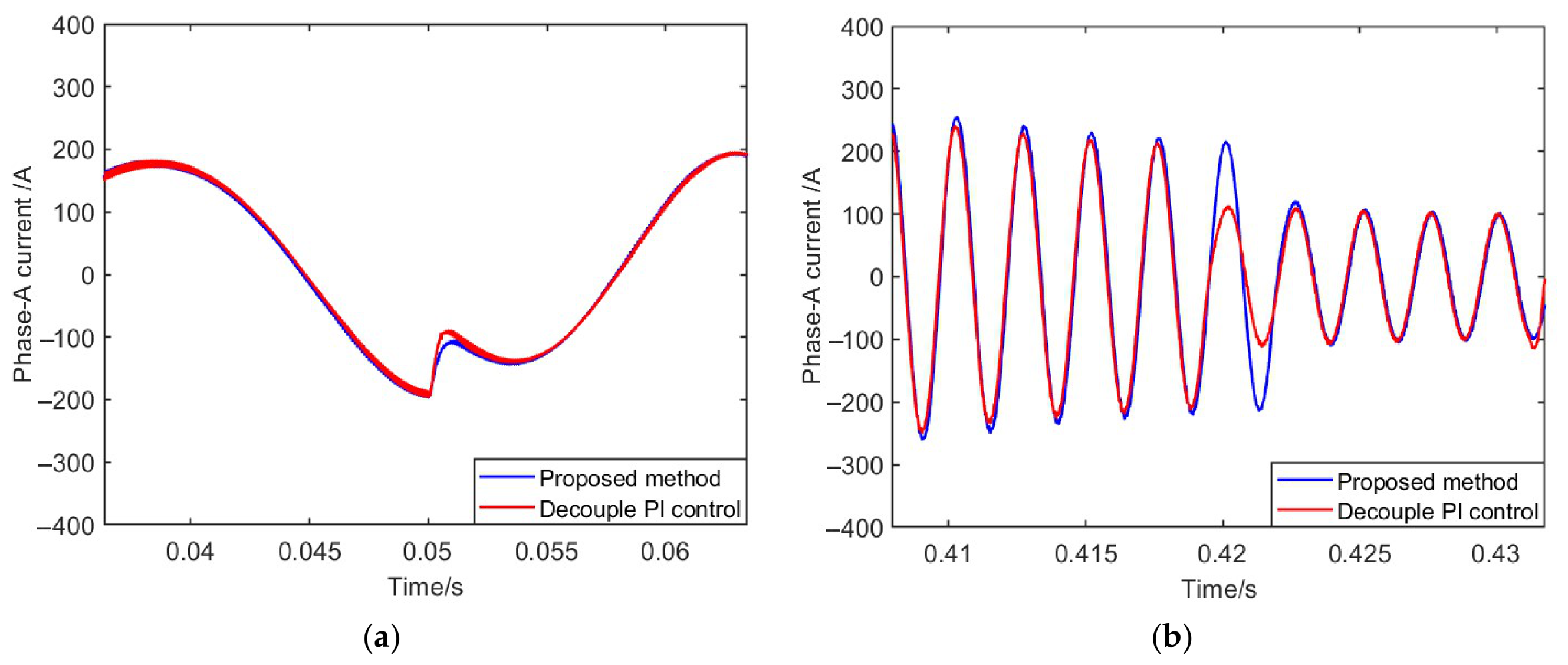
Figure 21 shows the variation in the motor’s phase-A winding current during operation. It can be observed that. At 0.05 s, the phase-A current deviates due to the change in load torque, and the deviation generated by the decoupled PI control at this point is significantly larger than that of the proposed method. Furthermore, at 0.42 s, a current transient occurs due to the motor switching between the two stator current planning algorithms. It can be seen that the smoothness of the current transition using the proposed method is superior to that of the decoupled PI control.

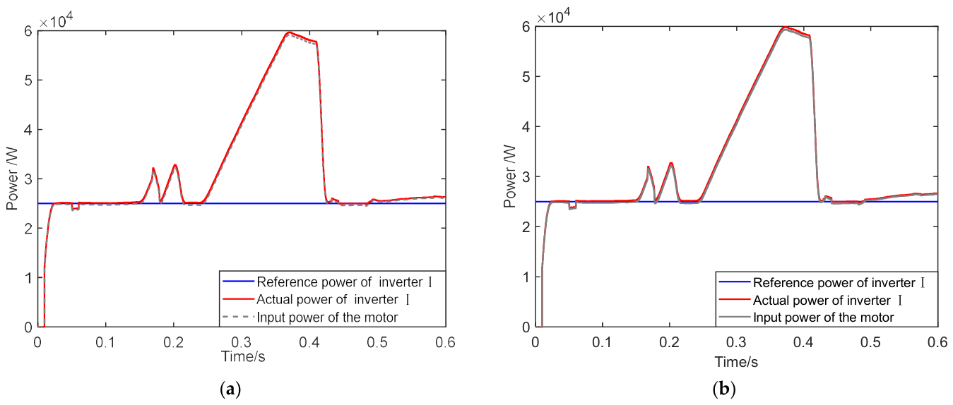
During the simulation process, the requested power of the inverter I, the actual input power of the inverter I, and the motor input power are shown in Figure 22. Since the main difference between the two algorithms lies in the stator voltage vector, and the two sets of stator current planning algorithms used are identical, the inverter power allocation is the same in both groups. Additionally, the operating conditions for both groups are identical. Therefore, the steady-state errors and transient behaviors of the two algorithms are generally the same. Furthermore, it can be observed that when the stator current algorithm switches from LMA to MPAR, the power allocated by the inverter increases. This similarly validates that the power allocation range of the MPAR is superior to that of the LMA.

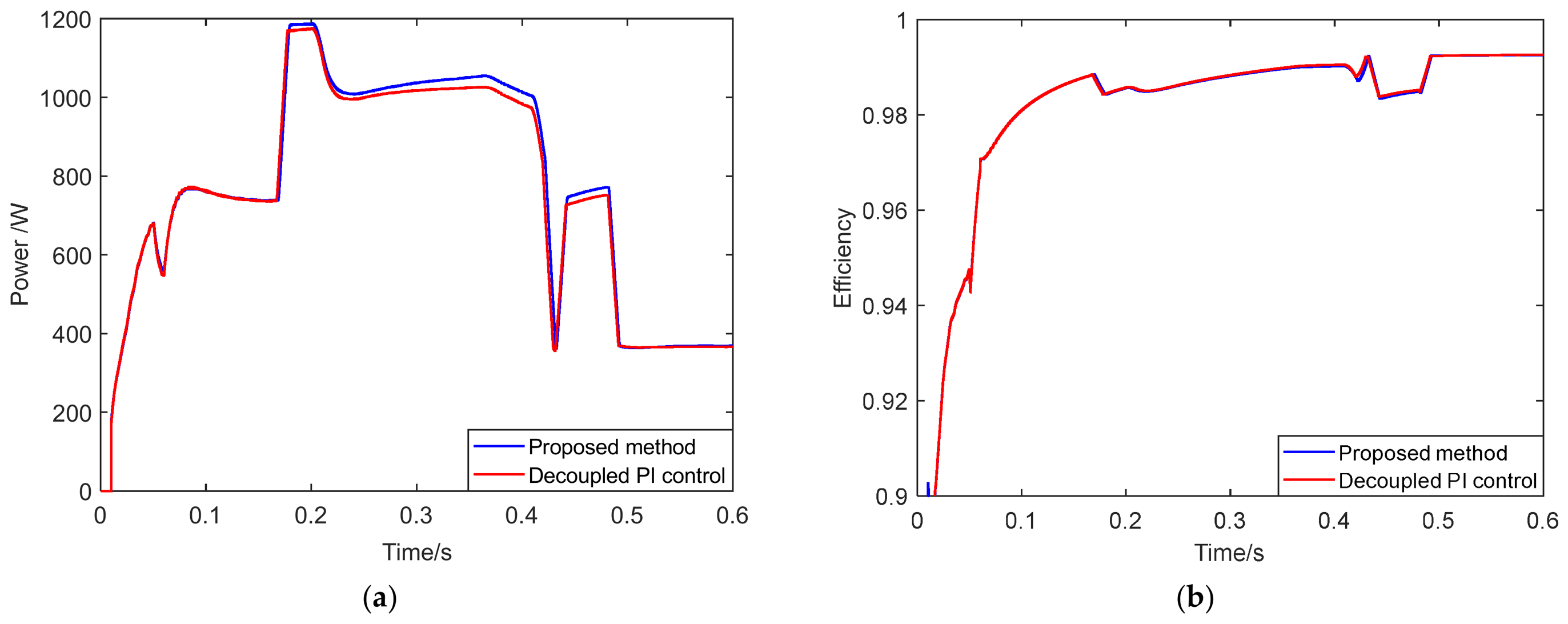
The power loss and efficiency of the motor under the two algorithms are shown in Figure 23a and Figure 23b, respectively. In the early stage of the simulation, the power loss of the two groups is generally consistent. Around 0.2 s, the motor switches from the LMA to the MPAR, resulting in a significant increase in power loss and a slight decrease in efficiency. After 0.5 s, the motor switches back to the LMA, causing the power loss to drop sharply and the motor efficiency to increase and remain constant. Therefore, it can be concluded that the LMA is more effective in reducing electrical losses.

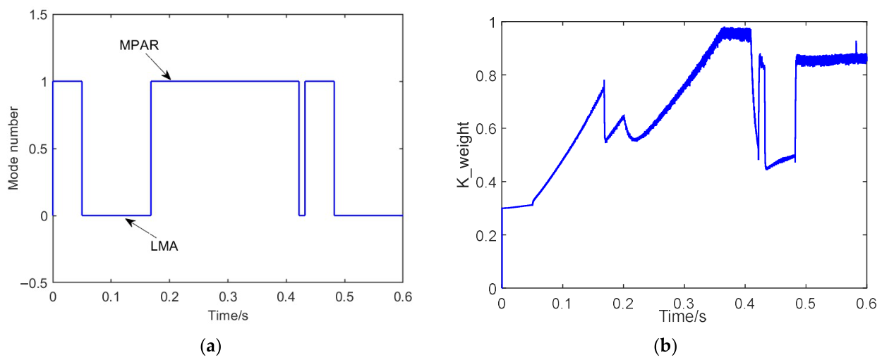
The stator current planning algorithm used during the operation of the proposed method is shown in Figure 24a. Figure 24b shows the variation in the weight coefficient $K_{weight}$ during the simulation process, which represents how close the stator voltage amplitude is to the maximum voltage amplitude $u_{s\max }$. When the stator current algorithm switches, the value of $K_{weight}$ also undergoes a sudden change. During the motor acceleration and load transient phases, the $K_{weight}$ value rises rapidly, approaching but always remaining less than 1. This indicates that the system is actively approaching the boundary of the voltage limit circle to respond to power demands, while the proposed voltage planning algorithm effectively constrains the voltage vector within the circle. Therefore, it can be demonstrated that the motor’s operating state during the entire process never exceeds the limits defined by the MPAR, ensuring control stability.

In summary, during the simulation phase, the stator voltage vector allocation algorithm proposed in this paper demonstrates superior tracking performance and stability for motor speed and torque compared to the decoupled PI control algorithm. Therefore, the innovative algorithm proposed in this paper enables real-time transient control of motor torque and current, satisfying the requirements for electromagnetic torque tracking and current transient response during motor operation, thereby enhancing the stability of system operation.

5.3. Experimental Results and Comparative Analysis

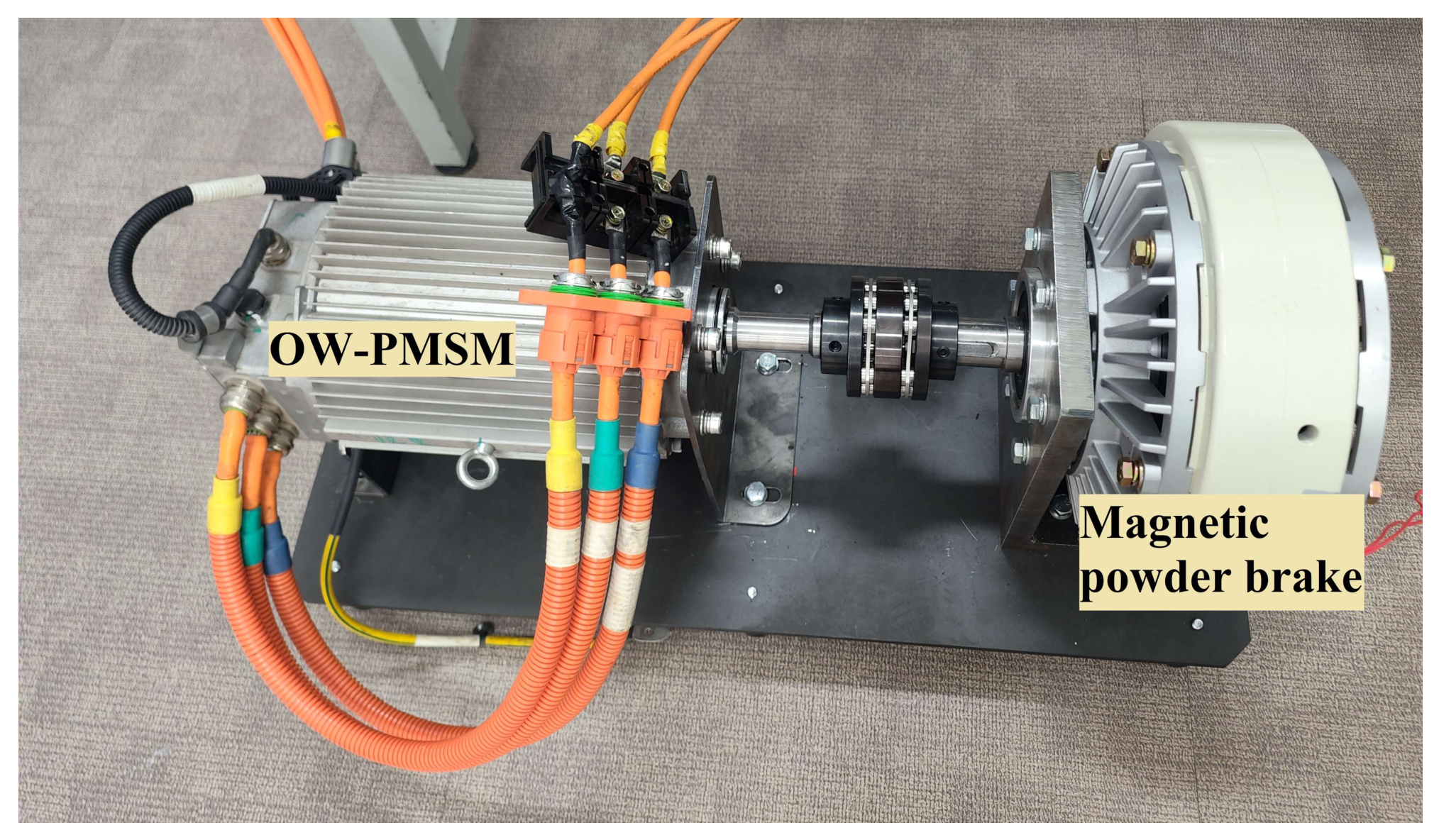
An experimental setup was built to experimentally validate the proposed scheme, as shown in Figure 25:

The motor state parameters are presented in

Table 3. Parameters of the experimental hardware platform.

Hardware	Parameter	Value
OW-PMSM	$\mathrm{Rotor}\mathrm{pole}\mathrm{pairs}{p}_0$	4
	$\mathrm{Armature}\mathrm{resistance}{R}_s/\Omega$	1.5
	$\mathrm{Equivalent}\mathrm{iron}\mathrm{loss}\mathrm{resistance}{R}_c/\Omega$	900
	$\mathrm{Permanent}\mathrm{magnet}\mathrm{flux}\mathrm{linkage}{\psi }_f/\mathrm{Wb}$	0.26
	$\mathrm{Stator}\mathrm{inductance}\mathrm{of}\mathrm{d}\text{-}\mathrm{axis}{L}_d/\mathrm{H}$	28 × 10−3
	$\mathrm{Stator}\mathrm{inductance}\mathrm{of}\mathrm{q}\text{-}\mathrm{axis}{L}_q/\mathrm{H}$	39 × 10−3
	$\mathrm{Maximum}\mathrm{phase}\mathrm{current}{i}_{p\max }/\mathrm{A}$	10
	$\mathrm{Nominal}\mathrm{phase}\mathrm{voltage}{u}_{p\max }/\mathrm{V}$	220
DC sources	$\mathrm{DC}1\mathrm{voltage}{U}_{dc1}/\mathrm{V}$	150
	$\mathrm{DC}2\mathrm{voltage}{U}_{dc2}/\mathrm{V}$	150

.

The parameters used for the experimental group and the control group are listed in

Table 4. Controller parameters of the proposed method and decoupled PI control for experiment.

Item	Parameter	Value
Proposed method	$\mathrm{Breakpoint}\mathrm{array}\mathrm{of}{k}_{Te}$	[0, 0.25, 0.5, 0.75, 1.25, 2.5, 5]
	$\mathrm{Data}\mathrm{of}{k}_{Te}$	[0, 250, 750, 1500, 3000, 5000, 6000]
	$\mathrm{d}\text{-}\mathrm{axis}\mathrm{current}\mathrm{gain}\mathrm{coefficient}{k}_{id}$	800
Decoupled PI control	$\mathrm{Proportion}\mathrm{coefficient}{K}_P$	10
	$\mathrm{Integration}\mathrm{coefficient}{K}_I$	50
Others	$\mathrm{Sampling}\mathrm{period}/\mathrm{ms}$	0.5
	$\mathrm{Control}\mathrm{period}/\mathrm{ms}$	0.5
	$\mathrm{SVPWM}\mathrm{frequency}/\mathrm{kHz}$	2

.

To verify the stability of the proposed scheme, experiments were conducted under both high-speed (motor speed of 2000 r/min) and low-speed (motor speed of 1000 r/min) operating conditions. The experiment duration was 200 ms. A load torque of 3 Nm was applied to both groups from 0 to 70 ms, which then abruptly changed to 6 Nm at 70 ms and remained constant until the end. From 0 to 20 ms, both groups used the LMA. At 20 ms, the current planning algorithm switched to MPAR until 120 ms, at which point it switched back to the LMA.

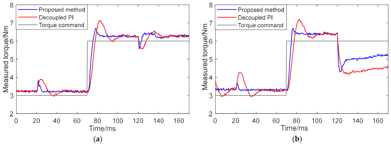
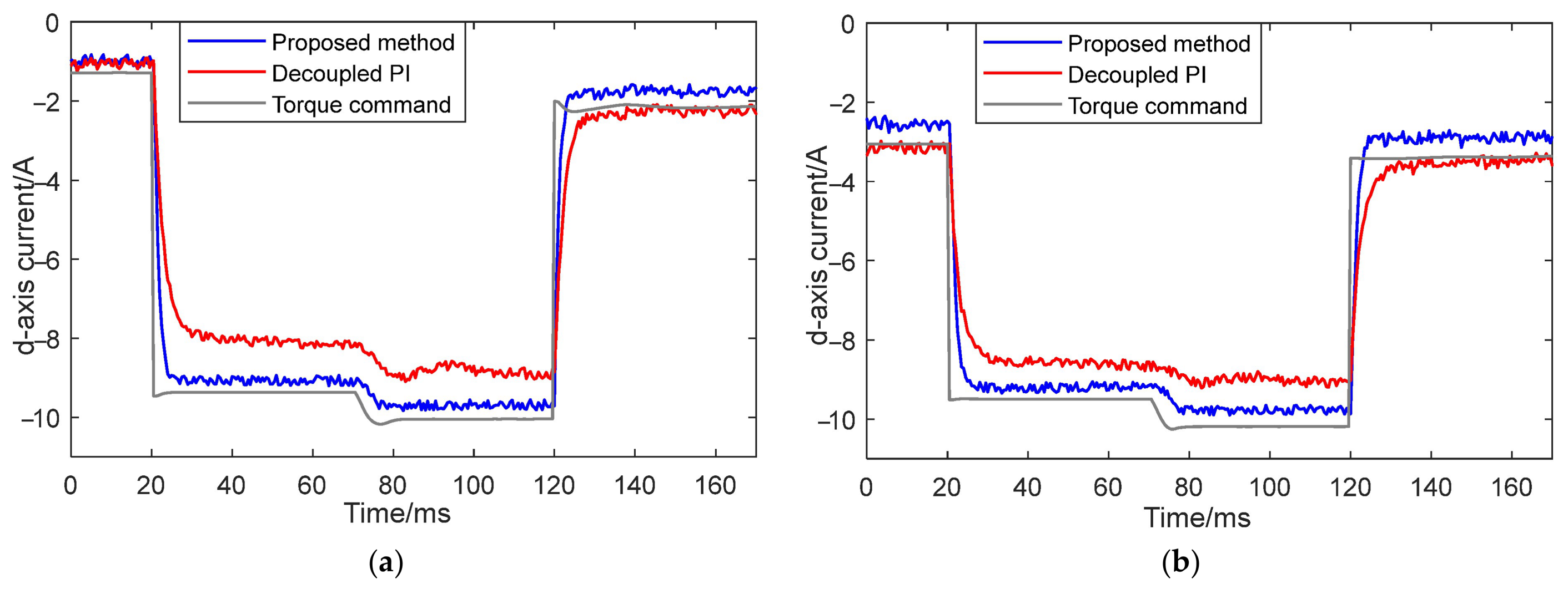
The actual electromagnetic torque and d-axis current results for the two groups during the experiment are shown in Figure 26 and Figure 27, respectively. Quantitative torque tracking performance metrics are listed in

Table 5. Comparison of torque tracking between the experimental and control groups.

Item	Parameter	Low Speed	High Speed
Experimental group	Mean tracking error/Nm	0.164	0.274
	Maximum tracking error/Nm	2.825	2.733
	Root mean squared error/Nm	0.515	0.531
	Standard deviation/Nm	0.489	0.456
Control group	Mean tracking error/Nm	0.168	0.251
	Maximum tracking error/Nm	2.838	2.737
	Root mean squared error/Nm	0.664	0.686
	Standard deviation/Nm	0.644	0.640

.

Under low-speed operating conditions, as shown in Figure 26a, a torque fluctuation occurs at 0.02 s due to the switching of the stator current algorithm. At this point, the algorithm proposed in this paper exhibits a faster response rate and a smaller fluctuation amplitude compared to the decoupled PI control. At this same moment, the stator current also undergoes a sudden change. It is clear in Figure 27a that the proposed algorithm has a faster response rate during the current transient, and the steady-state error in the subsequent operation is significantly improved compared to the decoupled PI control.

When the motor operates under high-speed conditions, a switching of the stator current algorithm mode also occurs at 20 ms, as shown in Figure 26b and Figure 27b. Near this switching, the electromagnetic torque of the decoupled PI control group frequently exhibits large fluctuations, and the system is unable to reach a stable operating state. In contrast, the method proposed in this paper enables the system to enter a stable operating state relatively quickly during this phase, and the fluctuation amplitude generated during the stator current algorithm switching is smaller. Furthermore, at 120 ms, the configuration switches the stator current algorithm again. After this switch, the decoupled PI control group exhibits a significant steady-state error, while the proposed scheme demonstrates a faster response rate at this moment. For the d-axis current, the algorithm proposed in this paper overall also exhibits smaller steady-state errors and a faster response rate.

Based on the error conditions shown in Table 5, under the control of the proposed algorithm, the maximum tracking error, root mean square error, and standard deviation of the electromagnetic torque are all smaller than those of the decoupled PI control, while the mean tracking error is almost comparable to that of the decoupled PI control. The reduction in settling time signifies a substantially faster dynamic response. The drastic decrease in maximum overshoot represents a major improvement in transient stability and smoother mode switching. The lower steady-state error and torque ripple indicate enhanced tracking accuracy and smoother operation. This demonstrates that during torque transients caused by current algorithm switching, the proposed algorithm can more effectively limit the amplitude of torque fluctuations and achieve a smaller ripple amplitude across the entire operating range, thereby ensuring stability during algorithm transitions.

In summary, the stator voltage vector allocation algorithm proposed in this paper exhibits small steady-state error, a faster response rate, and a smaller fluctuation amplitude during stator current algorithm switching. It achieves stable tracking of the electromagnetic torque, endowing the system with better robustness.

5.4. Limitations and Future Work

The above subsection verifies the reliability of the proposed algorithm in the dual-inverter OW-PMSM through comparative simulations and experiments. However, the overall analysis still has the following limitations. First, during the modeling process, the energy sources are assumed to provide ideal and balanced DC power, without considering possible voltage imbalances or differences in source impedance. This may have an impact on dynamic power allocation. Second, both the simulations and experiments employ fixed motor parameters, without accounting for parameter variations or thermal effects during motor operation, and no evaluation of the algorithm’s robustness against parameter changes or thermal effects is conducted. Furthermore, experiments are carried out on a static test bench, so the influence of vehicle operating parameters on the system cannot be considered.

It should be noted that the primary focus of the current research is to determine the reliability and performance comparison of the core methods within the control framework under steady-state or controllable conditions. In contrast, the study of system reliability under the aforementioned non-ideal and time-varying real-world scenarios is identified as a key direction for future research before practical application.

6. Conclusions

This paper focuses on OW-PMSM drive system for electric vehicles, optimizing its stator current planning algorithms and dynamic control performance. Firstly, two stator current planning algorithms are proposed. Among them, the Loss Minimization Algorithm (LMA) focuses on minimizing the electrical losses during motor operation, while the Maximum Power Allocation Range Algorithm (MPAR) aims to maximize the power allocation range of the dual inverters. Based on this, a geometric algorithm for stator voltage vector allocation is proposed. The voltage vector dynamically coordinates the gain requirements of electromagnetic torque and d-axis current based on the steady-state voltage saturation, thereby ensuring that the stator current follows the optimization results and preventing the motor from becoming unstable near its characteristic limits. This algorithm optimizes the tracking characteristics of the d-axis current and torque during motor operation while ensuring a low computational burden, thereby improving system stability. Subsequently, the proposed algorithm is compared with traditional decoupled PI control through simulations and experiments, validating its practical performance and feasibility. In future work, the proposed scheme can be implemented on more advanced embedded hardware to conduct more comprehensive theoretical stability verification, while exploring synergies with other multi-energy combinations.