Figure 1.
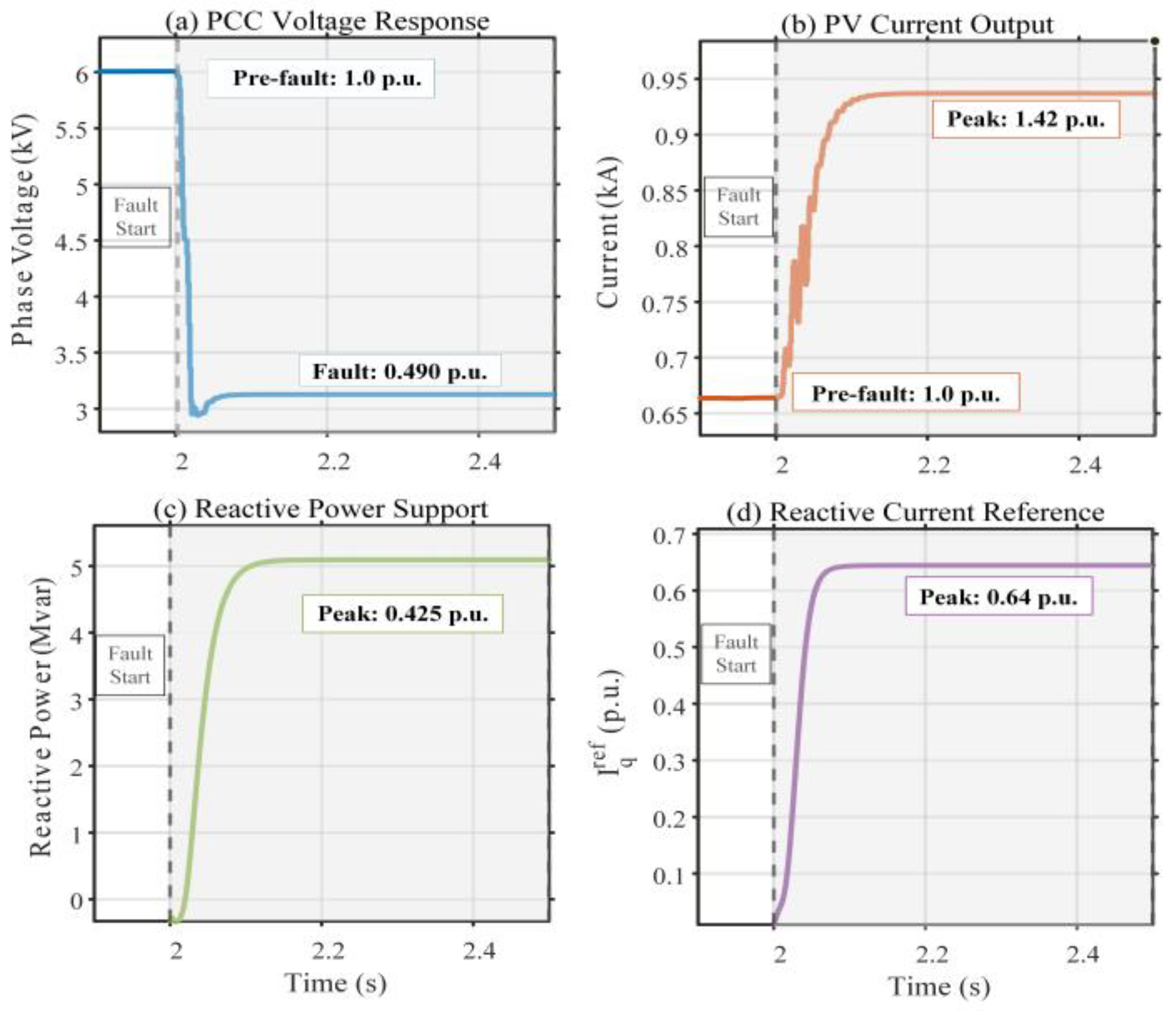
Distributed PV Dynamic Response Validation. (a) quantitatively characterizes the dynamic voltage sag characteristics at PCC Phase A, demonstrating an abrupt descent from the rated operating condition (1.0 p.u.) to 0.517 p.u., reflecting the severity of the grid disturbance. (b) reveals the overcurrent limiting mechanism of the PV inverter, where the output current rapidly increases from the rated value (1.0 p.u.) to 1.409 p.u. before stabilization, manifesting the controlled source characteristics of distributed PV. (c) demonstrates the effectiveness of the inverter’s low-voltage ride-through (LVRT) strategy, showing a significant increase in reactive power output from 0 to 5 Mvar (0.417 p.u.), thereby confirming its voltage support capability during grid disturbances. (d) elucidates the dynamic behavior of the internal reactive current reference command, transitioning from a steady-state zero value to −0.65 p.u., unveiling the voltage-sag-depth-based adaptive control strategy. This comprehensive analysis validates the coordinated operational mechanism of distributed PV systems, which simultaneously exhibit controlled current source characteristics and active voltage support functionality under grid fault conditions.
Figure 1.
Distributed PV Dynamic Response Validation. (a) quantitatively characterizes the dynamic voltage sag characteristics at PCC Phase A, demonstrating an abrupt descent from the rated operating condition (1.0 p.u.) to 0.517 p.u., reflecting the severity of the grid disturbance. (b) reveals the overcurrent limiting mechanism of the PV inverter, where the output current rapidly increases from the rated value (1.0 p.u.) to 1.409 p.u. before stabilization, manifesting the controlled source characteristics of distributed PV. (c) demonstrates the effectiveness of the inverter’s low-voltage ride-through (LVRT) strategy, showing a significant increase in reactive power output from 0 to 5 Mvar (0.417 p.u.), thereby confirming its voltage support capability during grid disturbances. (d) elucidates the dynamic behavior of the internal reactive current reference command, transitioning from a steady-state zero value to −0.65 p.u., unveiling the voltage-sag-depth-based adaptive control strategy. This comprehensive analysis validates the coordinated operational mechanism of distributed PV systems, which simultaneously exhibit controlled current source characteristics and active voltage support functionality under grid fault conditions.

Figure 2.
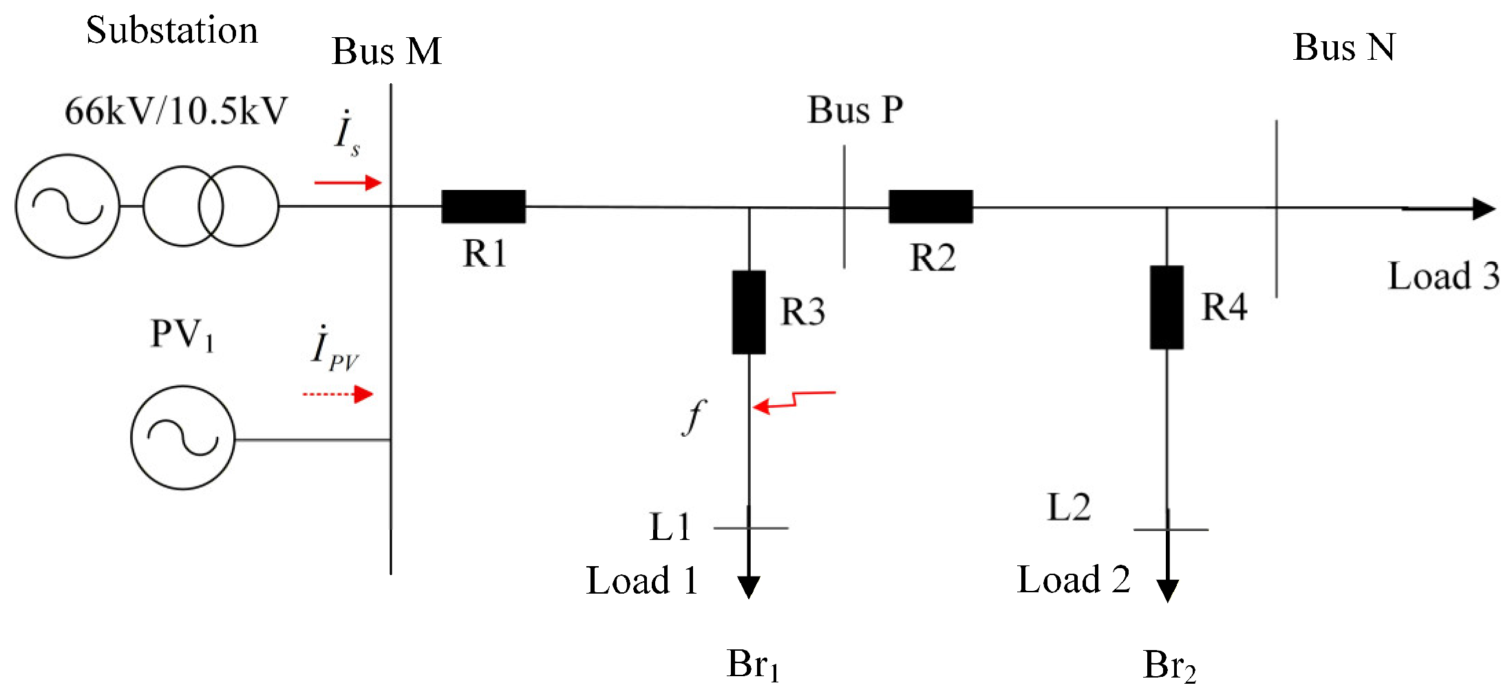
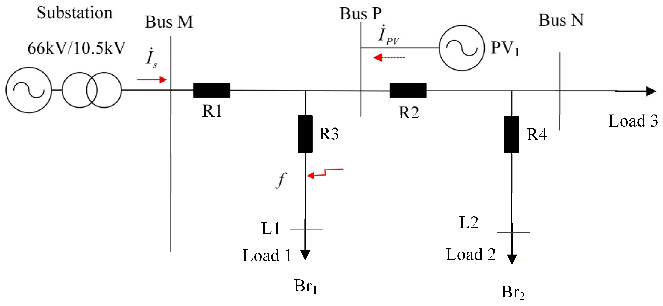
Typical fault scenario under PV fault current contribution.
Figure 2.
Typical fault scenario under PV fault current contribution.
Figure 3.
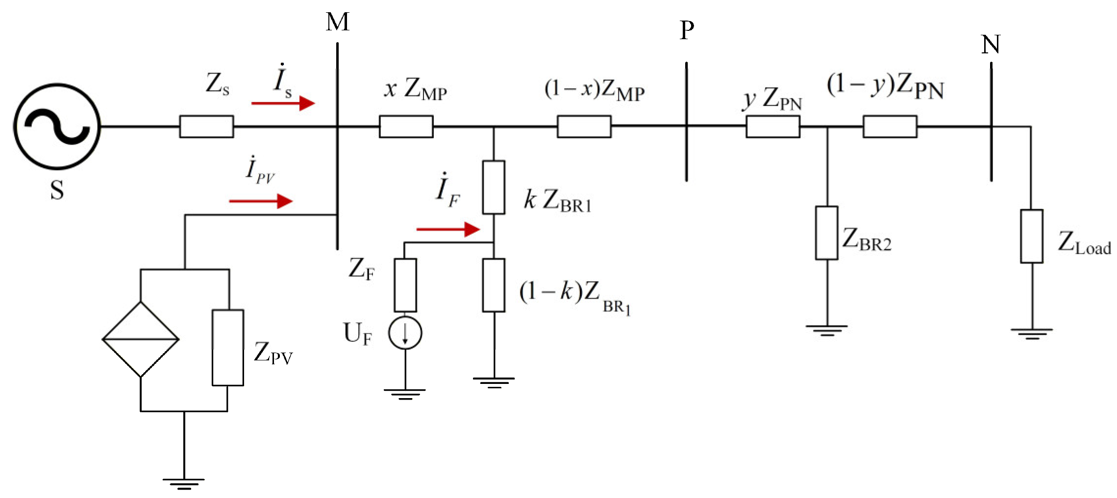
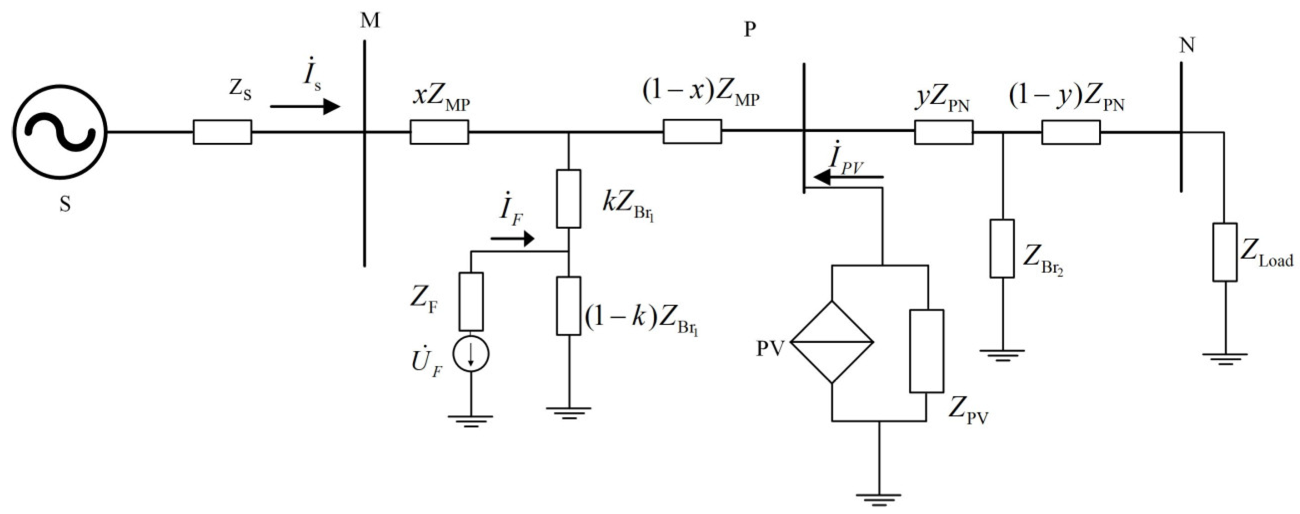
Positive-sequence equivalent model of a distribution network with PV fault current contribution.
Figure 3.
Positive-sequence equivalent model of a distribution network with PV fault current contribution.
Figure 4.
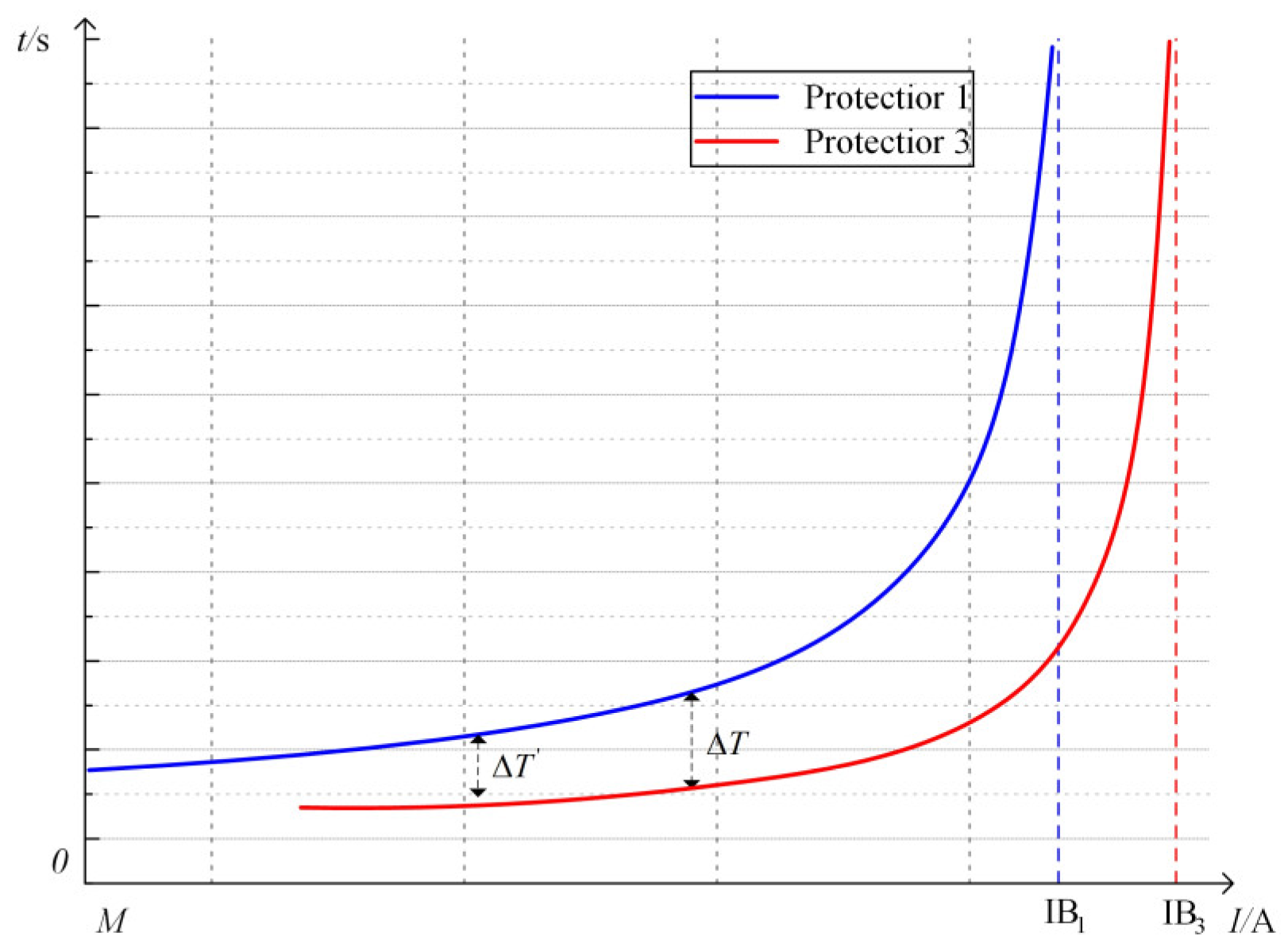
Protection operation time curve.
Figure 4.
Protection operation time curve.
Figure 5.
Typical fault scenario under PV fault current extraction.
Figure 5.
Typical fault scenario under PV fault current extraction.
Figure 6.
Positive-sequence equivalent circuit of the distribution network under a PV fault current extraction scenario.
Figure 6.
Positive-sequence equivalent circuit of the distribution network under a PV fault current extraction scenario.
Figure 7.
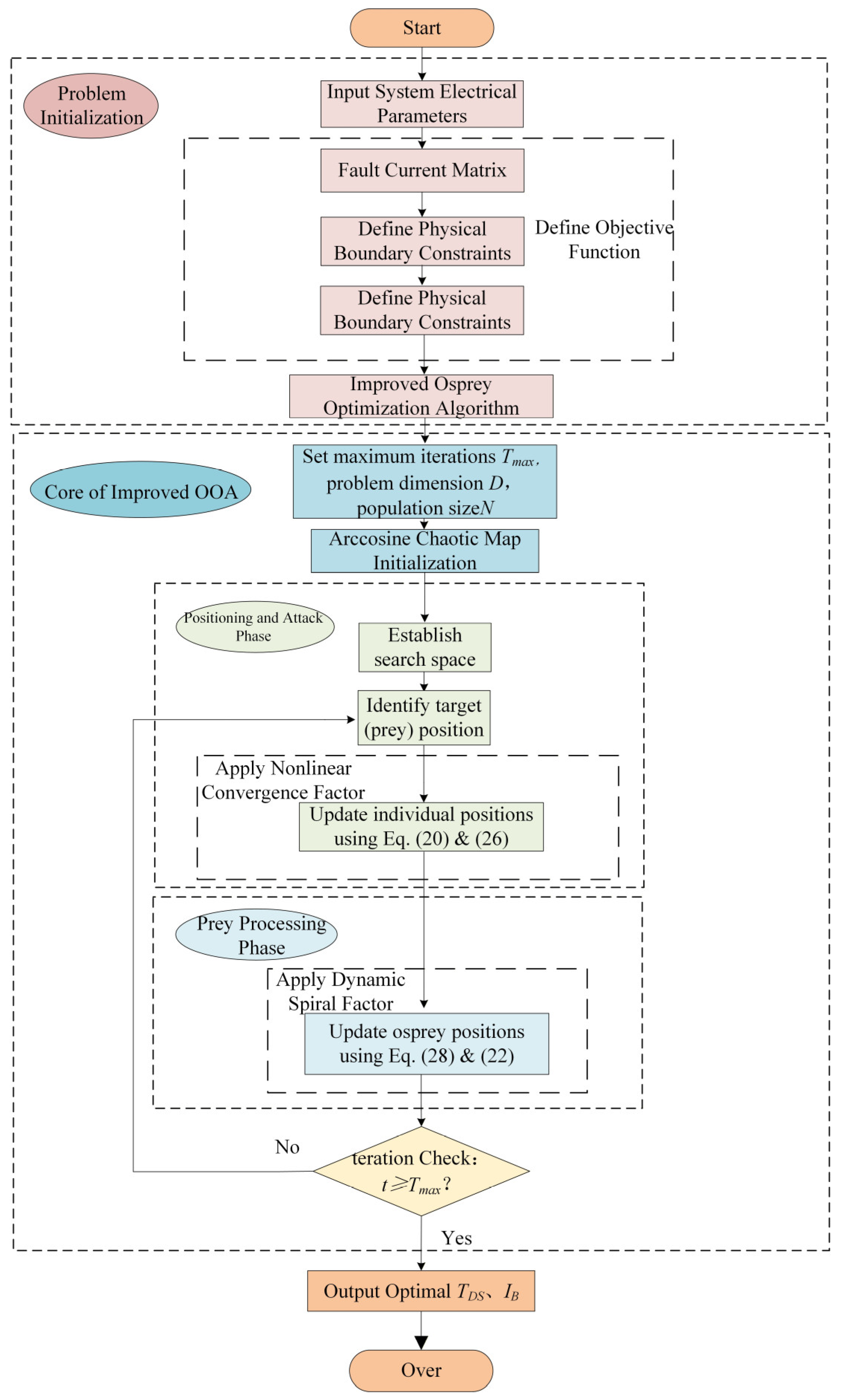
Flowchart of the improved osprey optimization algorithm.
Figure 7.
Flowchart of the improved osprey optimization algorithm.
Figure 8.
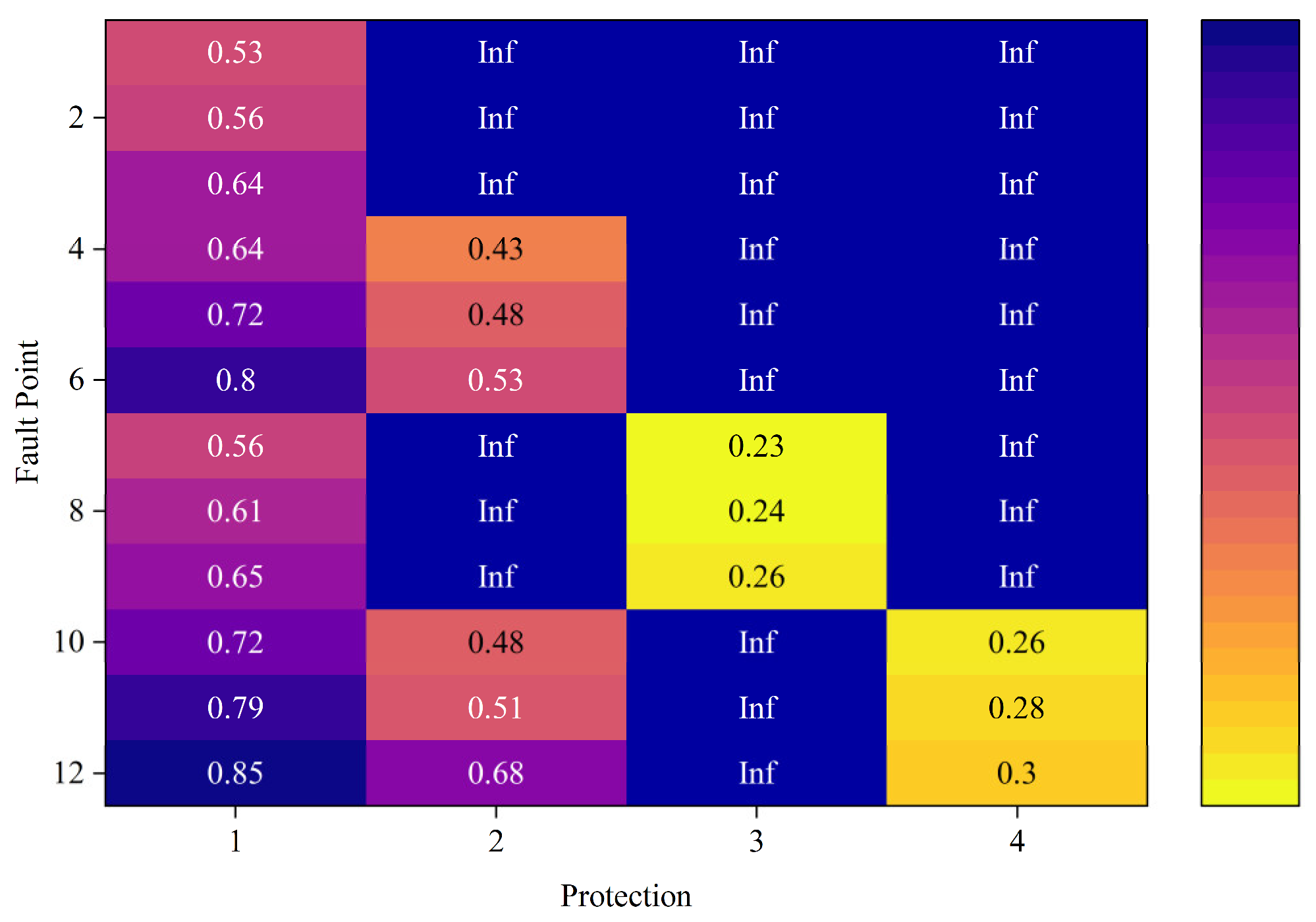
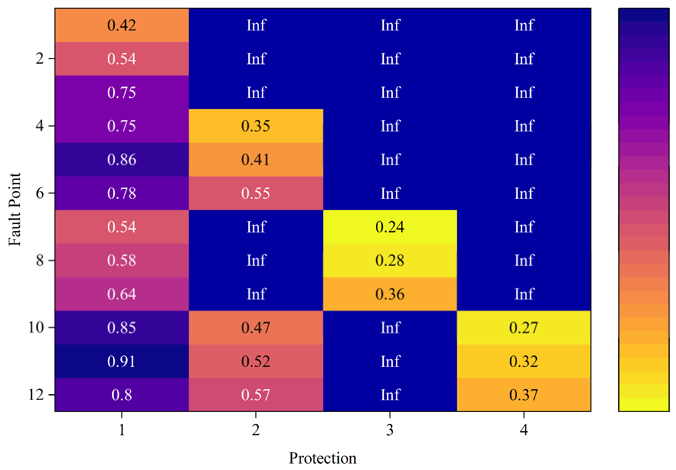
Heatmap of relay operating time under PV current contribution effect.
Figure 8.
Heatmap of relay operating time under PV current contribution effect.
Figure 9.
Heatmap of relay operating time under PV current extraction effect.
Figure 9.
Heatmap of relay operating time under PV current extraction effect.
Figure 10.
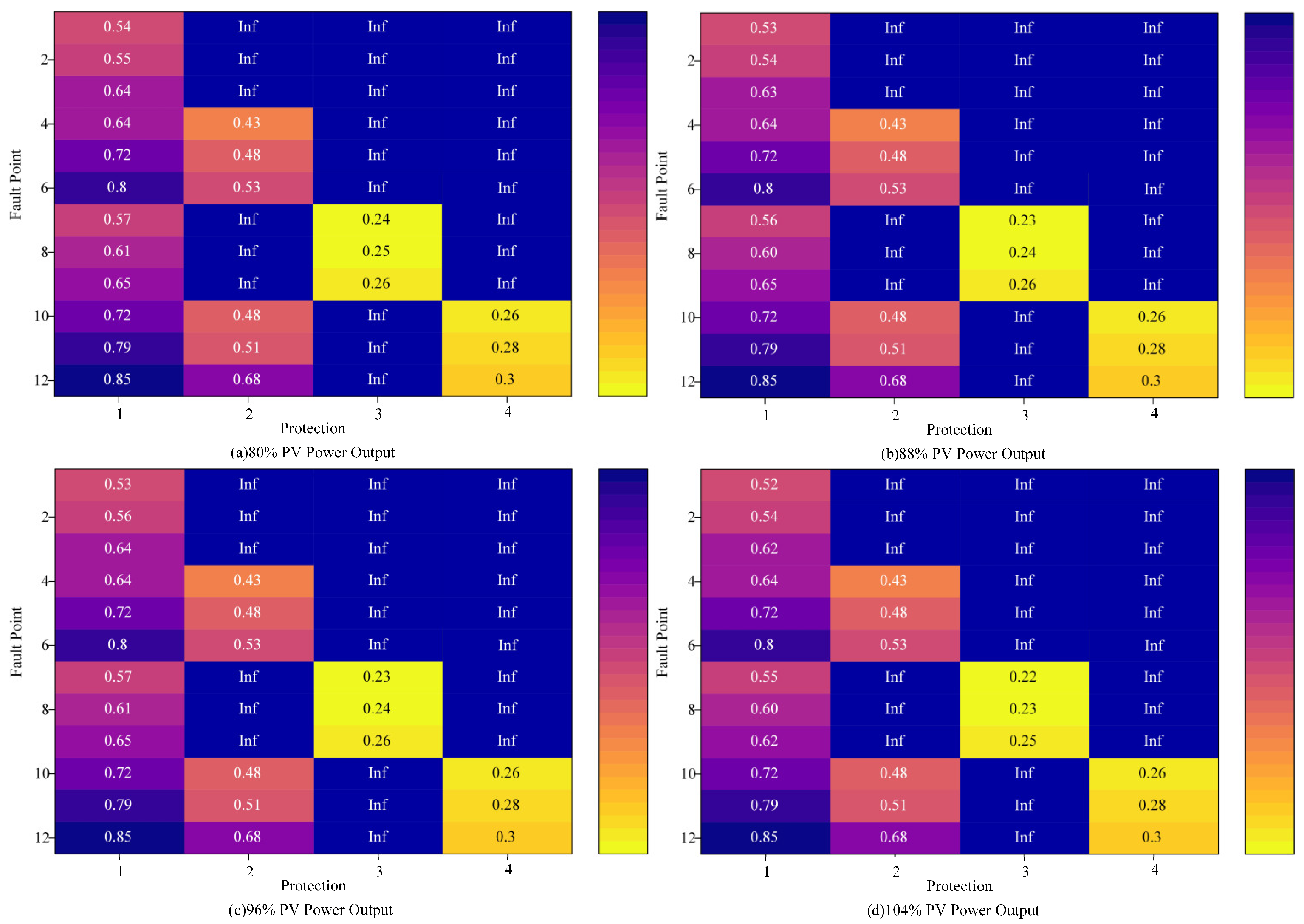
Heatmap of relay operating time under PV current contribution effect with output fluctuation. (a) illustrates the relay operating time distribution at 80% PV output, revealing a delayed response pattern in specific fault regions due to reduced current contribution. (b) depicts the operating behavior at 88% PV output, showing a progressive shortening of operation time in near-bus zones as PV penetration increases. (c) demonstrates the relay performance under 96% PV output, where the heatmap indicates a significant acceleration of operation across a wider fault distance range, approaching the relay setting threshold. (d) elucidates the operating characteristics at 104% PV output, highlighting a distinct zone of minimal operation time that expands outward from the substation, reflecting the enhanced current injection during over-generation conditions. This comprehensive analysis validates the sensitivity of relay operating time to varying levels of PV generation, underscoring the interplay between PV output fluctuation and protection coordination in distribution networks.
Figure 10.
Heatmap of relay operating time under PV current contribution effect with output fluctuation. (a) illustrates the relay operating time distribution at 80% PV output, revealing a delayed response pattern in specific fault regions due to reduced current contribution. (b) depicts the operating behavior at 88% PV output, showing a progressive shortening of operation time in near-bus zones as PV penetration increases. (c) demonstrates the relay performance under 96% PV output, where the heatmap indicates a significant acceleration of operation across a wider fault distance range, approaching the relay setting threshold. (d) elucidates the operating characteristics at 104% PV output, highlighting a distinct zone of minimal operation time that expands outward from the substation, reflecting the enhanced current injection during over-generation conditions. This comprehensive analysis validates the sensitivity of relay operating time to varying levels of PV generation, underscoring the interplay between PV output fluctuation and protection coordination in distribution networks.

Figure 11.
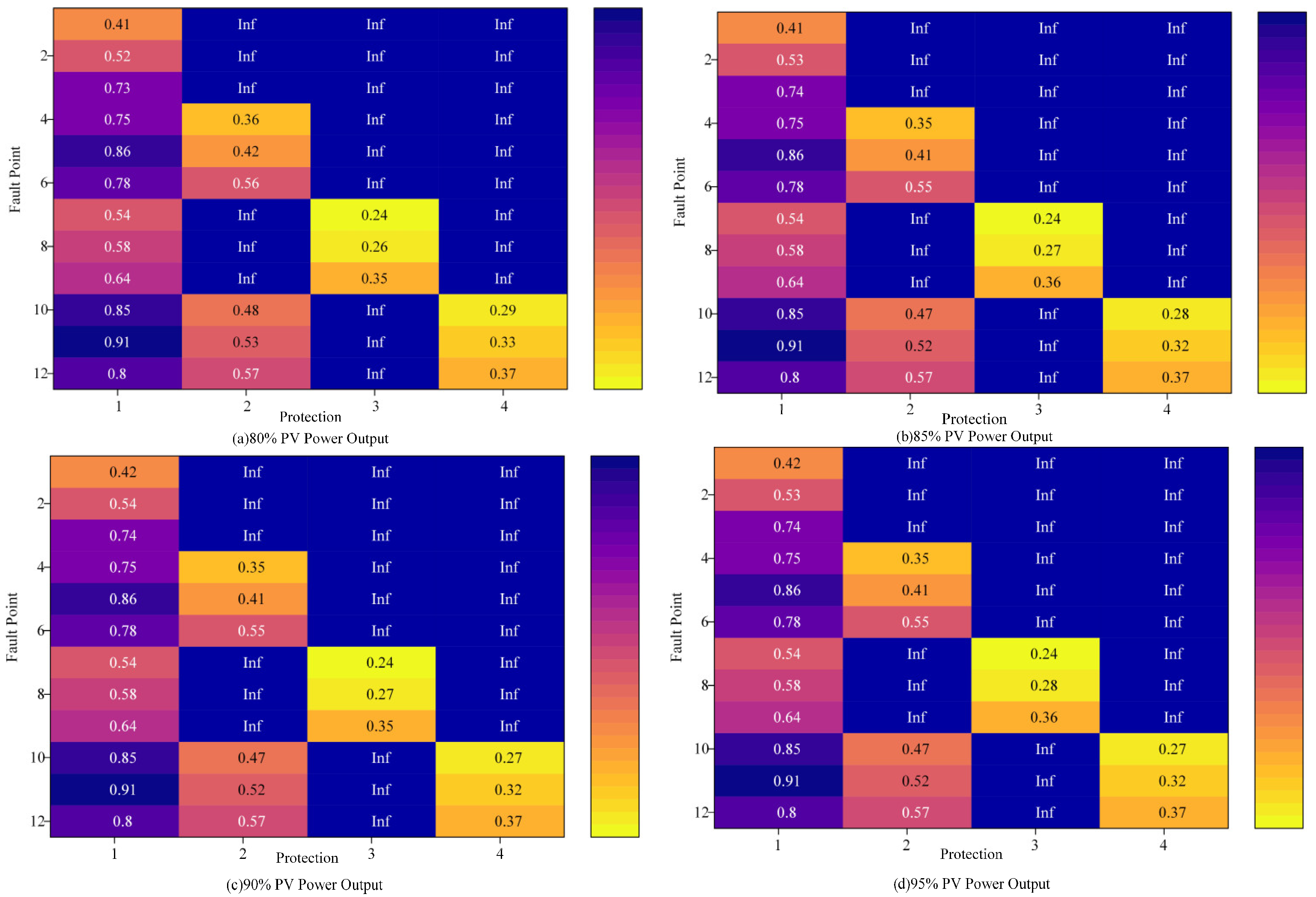
Heatmap of relay operating time under PV current extraction effect with output fluctuation. (a) presents the relay operating time distribution at 80% PV output, revealing a progressive delay in the operating time of the affected relays due to reduced fault current levels caused by current extraction. (b) depicts the operating characteristics at 85% PV output, showing a further extension of the relay operating time as the extraction effect intensifies. (c) demonstrates the relay performance under 90% PV output, where the heatmap indicates a significant and widespread increase in operating time. (d) illustrates the operating characteristics at 95% PV output, presenting a dominant region characterized by substantially delayed operation time. This highlights the substantial impact of high-level PV generation on fault current attenuation and protection system timing, while confirming that reliable operation is maintained overall. This comprehensive analysis verifies that the PV current extraction effect significantly prolongs relay operating time.
Figure 11.
Heatmap of relay operating time under PV current extraction effect with output fluctuation. (a) presents the relay operating time distribution at 80% PV output, revealing a progressive delay in the operating time of the affected relays due to reduced fault current levels caused by current extraction. (b) depicts the operating characteristics at 85% PV output, showing a further extension of the relay operating time as the extraction effect intensifies. (c) demonstrates the relay performance under 90% PV output, where the heatmap indicates a significant and widespread increase in operating time. (d) illustrates the operating characteristics at 95% PV output, presenting a dominant region characterized by substantially delayed operation time. This highlights the substantial impact of high-level PV generation on fault current attenuation and protection system timing, while confirming that reliable operation is maintained overall. This comprehensive analysis verifies that the PV current extraction effect significantly prolongs relay operating time.

Figure 12.
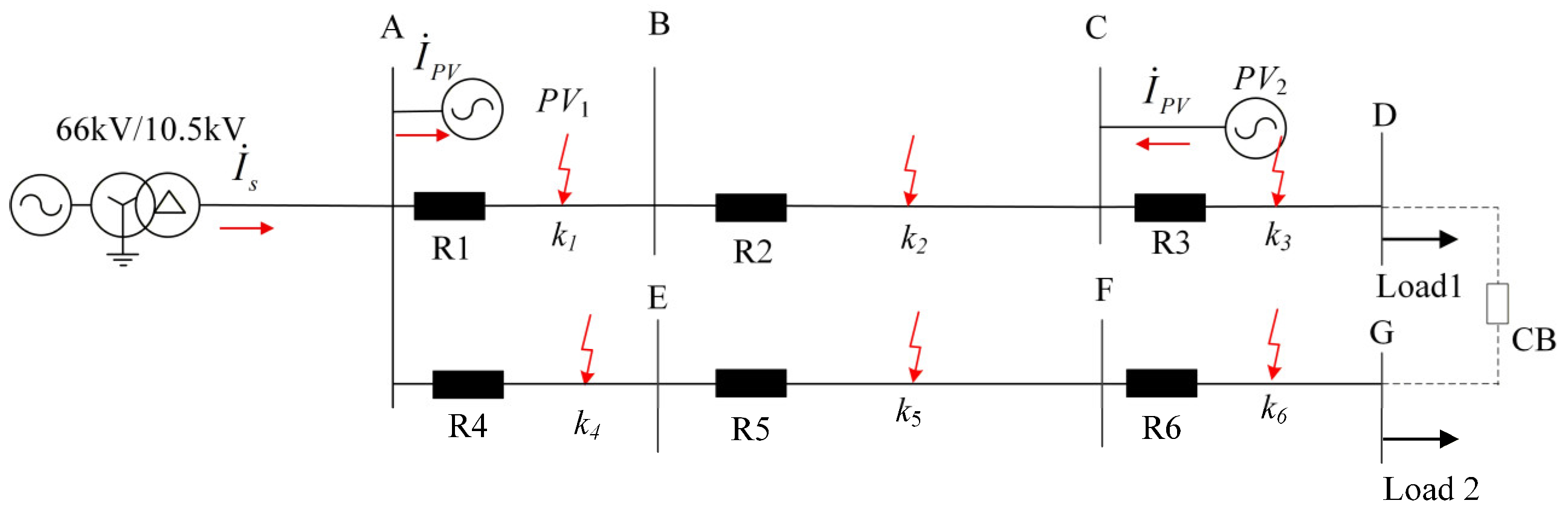
Single-line diagram of a dual-feeder distribution network with distributed PV.
Figure 12.
Single-line diagram of a dual-feeder distribution network with distributed PV.
Figure 13.
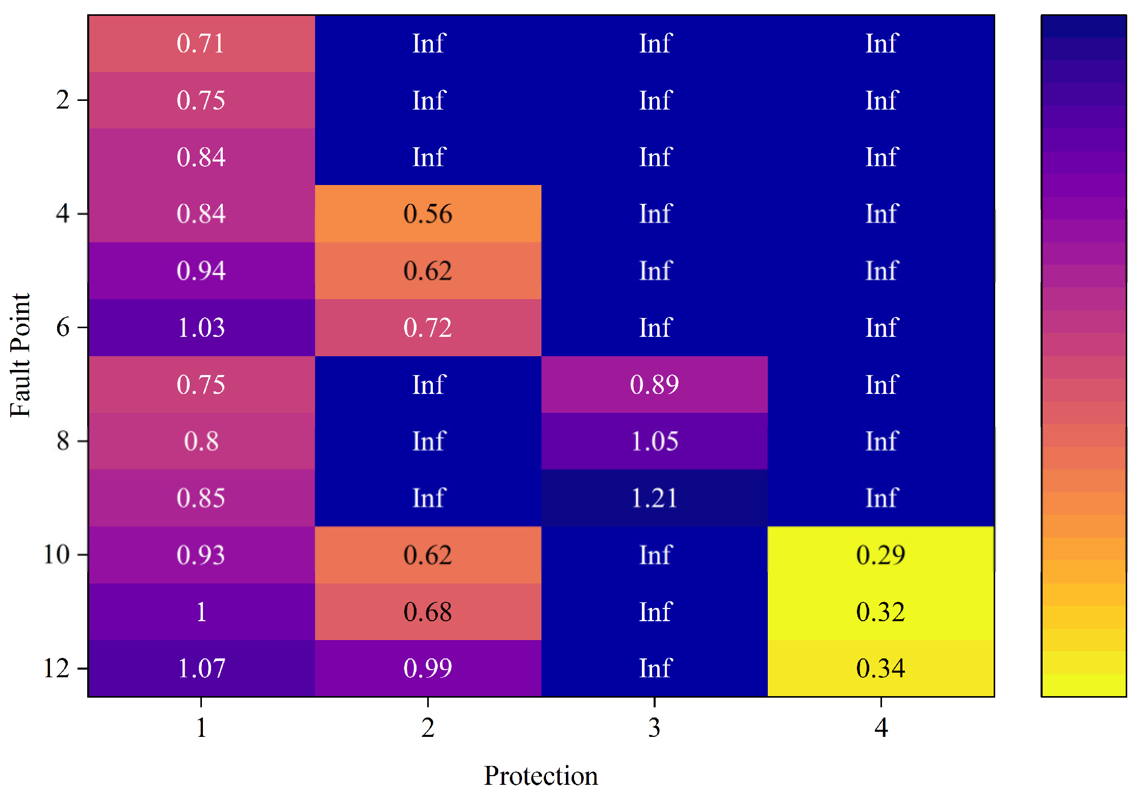
Heatmap of relay operating time based on original OOA under PV current contribution effect.
Figure 13.
Heatmap of relay operating time based on original OOA under PV current contribution effect.
Figure 14.
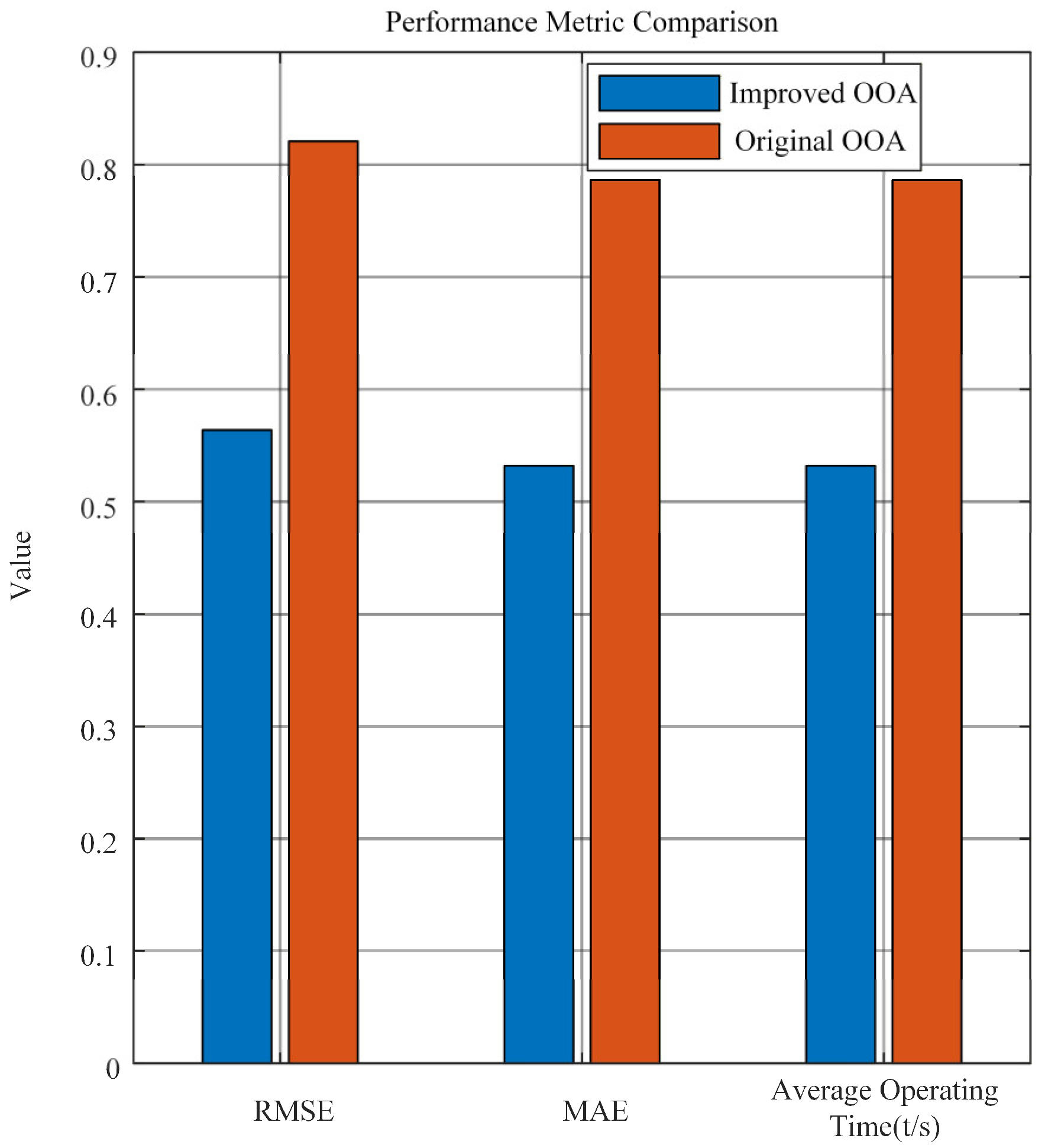
Performance and Error Comparison between Improved and Original Algorithms under PV Current contribution Effect.
Figure 14.
Performance and Error Comparison between Improved and Original Algorithms under PV Current contribution Effect.
Figure 15.
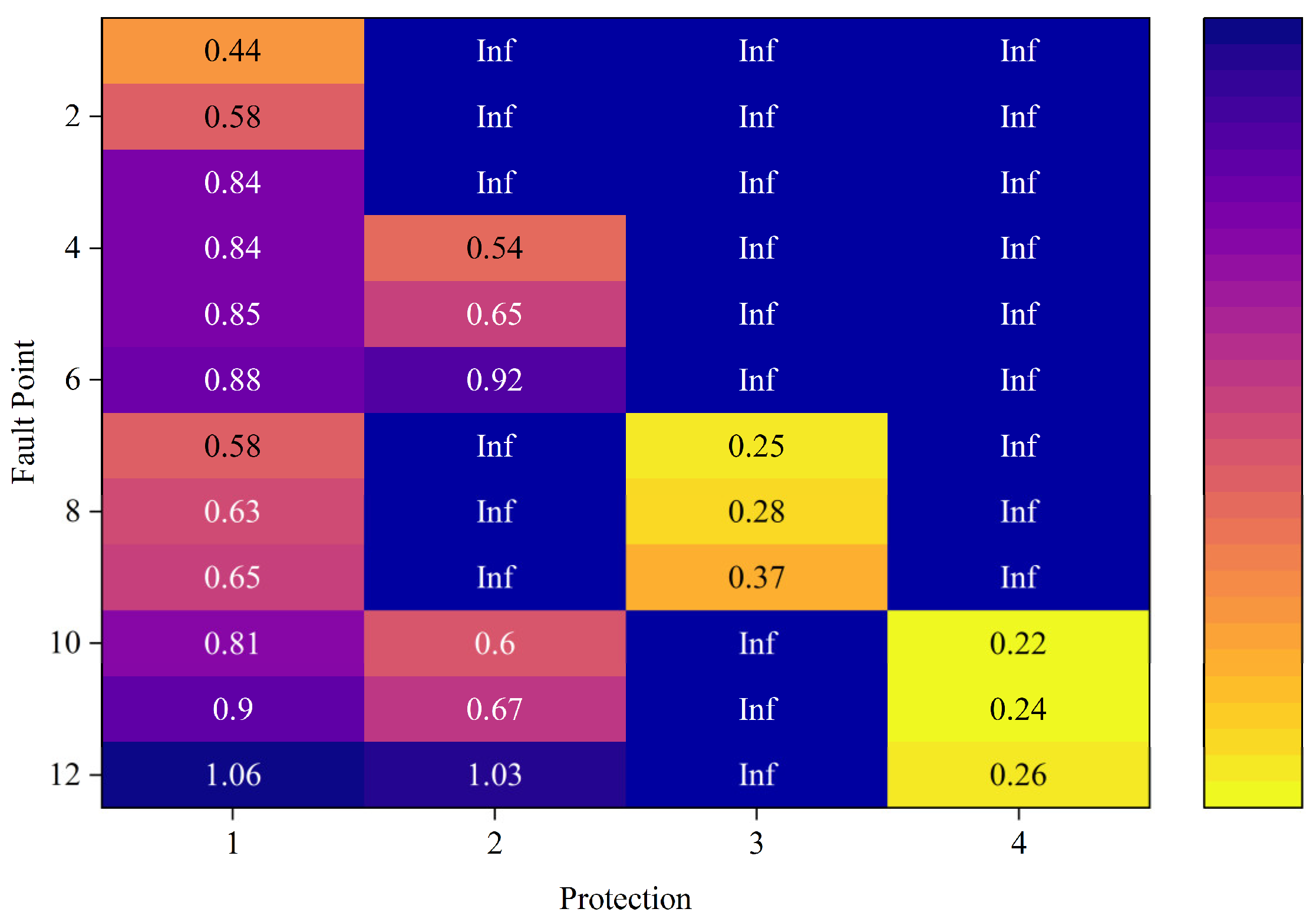
Heatmap of relay operating time based on original OOA under PV current extraction effect.
Figure 15.
Heatmap of relay operating time based on original OOA under PV current extraction effect.
Figure 16.
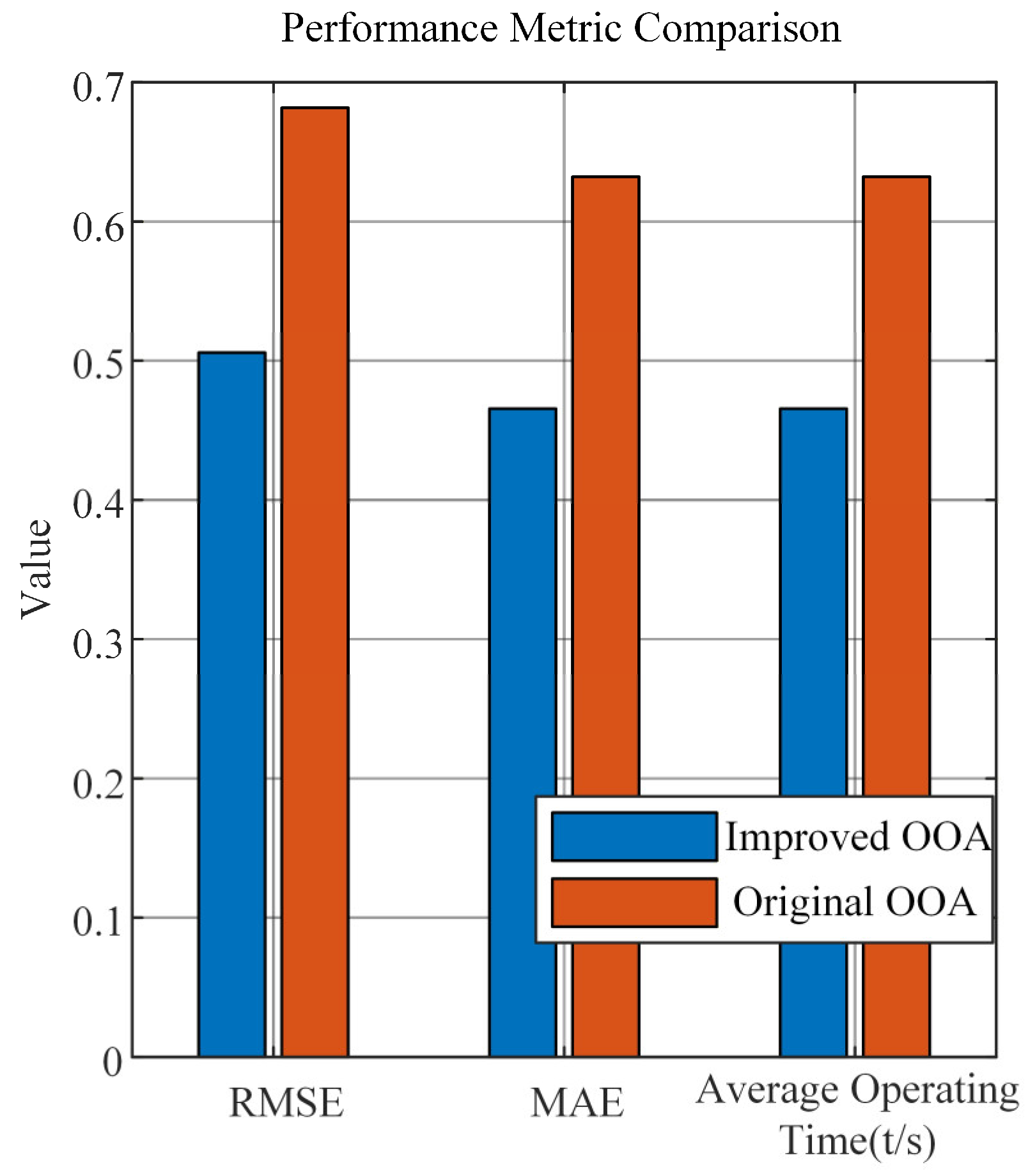
Performance and Error Comparison between improved and original algorithms under PV current extraction effect.
Figure 16.
Performance and Error Comparison between improved and original algorithms under PV current extraction effect.
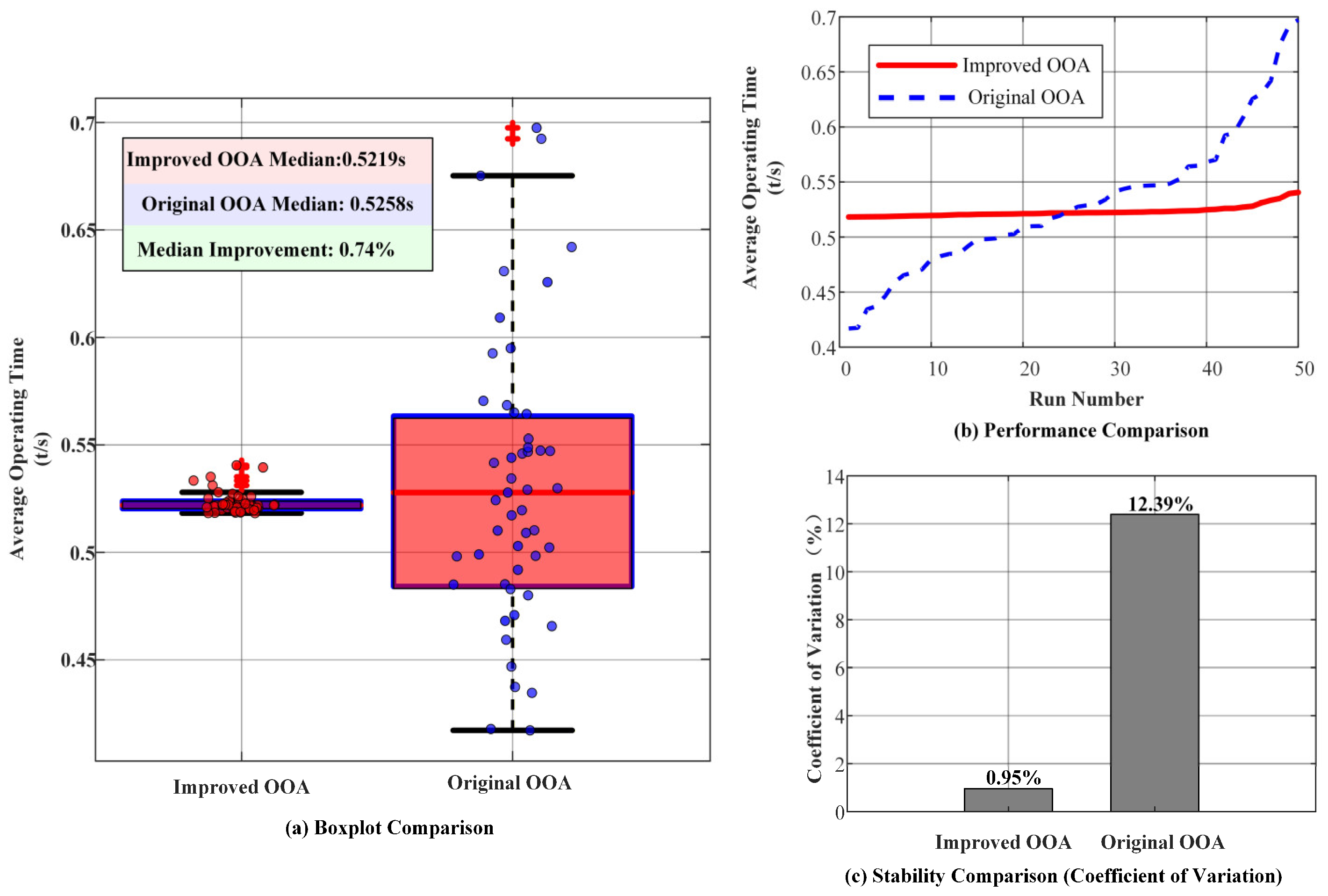
Figure 17.
Random initialization robustness verification results. (a) illustrates the distribution characteristics of the results from multiple runs of the two algorithms. The boxplot of the improved OOA for average operating time is narrower, more compact, and exhibits a smaller interquartile range compared to that of the original OOA, indicating higher consistency and effectively controlled dispersion of optimization results under different random initialization conditions. (b) reveals the differences in performance distribution patterns between the improved OOA and the original OOA. The improved OOA demonstrates a smaller performance fluctuation range, confirming its enhanced algorithmic stability. (c) provides quantitative confirmation of algorithm stability through a bar chart. The coefficient of variation for the improved OOA is significantly lower than that of the original OOA, statistically validating the reduced sensitivity of the improved algorithm to initial conditions and the reliability and repeatability of its output results. This comprehensive analysis verifies that the improved algorithm exhibits superior robustness and stable performance under random initialization conditions.
Figure 17.
Random initialization robustness verification results. (a) illustrates the distribution characteristics of the results from multiple runs of the two algorithms. The boxplot of the improved OOA for average operating time is narrower, more compact, and exhibits a smaller interquartile range compared to that of the original OOA, indicating higher consistency and effectively controlled dispersion of optimization results under different random initialization conditions. (b) reveals the differences in performance distribution patterns between the improved OOA and the original OOA. The improved OOA demonstrates a smaller performance fluctuation range, confirming its enhanced algorithmic stability. (c) provides quantitative confirmation of algorithm stability through a bar chart. The coefficient of variation for the improved OOA is significantly lower than that of the original OOA, statistically validating the reduced sensitivity of the improved algorithm to initial conditions and the reliability and repeatability of its output results. This comprehensive analysis verifies that the improved algorithm exhibits superior robustness and stable performance under random initialization conditions.

Table 1.
Line parameters of 10 kV distribution network.
Table 1.
Line parameters of 10 kV distribution network.
| Line | Length (km) | Conductor Specification | Positive-Sequence Impedance (Ω/km) | Zero-Sequence Impedance (Ω/km) |
|---|
| MP | 3.91 | YJV_240 | 0.069 + j0.099 | 0.110 + j0.159 |
| PN | 3.17 | YJV_240 | 0.069 + j0.099 | 0.110 + j0.159 |
| Br1 | 1.42 | YJV_120 | 0.106 + j0.153 | 0.169 + 0.245 |
| Br2 | 1.55 | YJV_120 | 0.106 + j0.153 | 0.169 + 0.245 |
Table 2.
Three-phase fault current matrix.
Table 2.
Three-phase fault current matrix.
| | Protection | R1 | R2 | R3 | R4 |
|---|
| Fault Point | |
|---|
| 1: MP Start Section | 8124 | 18 | 5 | 9 |
| 2: MP Middle Section | 7814 | 17 | 5 | 9 |
| 3: MP End Section | 6523 | 15 | 41 | 7 |
| 4: PN Start Section | 6524 | 6416 | 42 | 0 |
| 5: PN Middle Section | 5648 | 5664 | 58 | 6 |
| 6: PN End Section | 4809 | 4811 | 70 | 36 |
| 7: Br1 Start Section | 7801 | 18 | 7799 | 9 |
| 8: Br1 Middle Section | 6992 | 75 | 6989 | 38 |
| 9: Br1 End Section | 6393 | 132 | 6391 | 66 |
| 10: Br2 Start Section | 5623 | 5601 | 58 | 5603 |
| 11: Br2 Middle Section | 5611 | 5599 | 67 | 5600 |
| 12: Br2 End Section | 5201 | 5119 | 75 | 5117 |
Table 3.
Inverse-time overcurrent relay setting results under current contribution effect.
Table 3.
Inverse-time overcurrent relay setting results under current contribution effect.
| Setting Results | R1 | R2 | R3 | R4 |
|---|
| TDS | 0.14 | 0.11 | 0.07 | 0.07 |
| IB | 1273.7 | 961.5 | 762.2 | 692.4 |
Table 4.
BC-phase fault current matrix.
Table 4.
BC-phase fault current matrix.
| | Protection | R1 | R2 | R3 | R4 |
|---|
| Fault Point | |
|---|
| 1: MP Start Section | 8138 | 366 | 101 | 195 |
| 2: MP Middle Section | 5640 | 354 | 96 | 177 |
| 3: MP End Section | 3813 | 332 | 97 | 166 |
| 4: PN Start Section | 3819 | 8018 | 105 | 158 |
| 5: PN Middle Section | 3354 | 6263 | 110 | 6 |
| 6: PN End Section | 3670 | 4392 | 111 | 173 |
| 7: Br1 Start Section | 5632 | 351 | 9076 | 177 |
| 8: Br1 Middle Section | 5100 | 371 | 7788 | 199 |
| 9: Br1 End Section | 4874 | 380 | 5419 | 190 |
| 10: Br2 Start Section | 3346 | 6260 | 110 | 6056 |
| 11: Br2 Middle Section | 3193 | 5186 | 117 | 4831 |
| 12: Br2 End Section | 3577 | 4007 | 111 | 4107 |
Table 5.
Inverse-time overcurrent relay setting results under current extraction effect.
Table 5.
Inverse-time overcurrent relay setting results under current extraction effect.
| Setting Results | R1 | R2 | R3 | R4 |
|---|
| TDS | 0.11 | 0.09 | 0.06 | 0.06 |
| IB | 1371.7 | 1443.3 | 1829.3 | 1412.5 |
Table 6.
Simulation results under current contribution effect with different PV penetration ratios.
Table 6.
Simulation results under current contribution effect with different PV penetration ratios.
| PV Integration Capacity | R1 Operating Time (t/s) | R3 Operating Time (t/s) | |
|---|
| 12 MW | 0.56 | 0.24 | 0.34 |
| 6 MW | 0.63 | 0.28 | 0.35 |
| 0 MW | 0.67 | 0.31 | 0.36 |
Table 7.
Simulation results under current extraction effect with different PV penetration ratios.
Table 7.
Simulation results under current extraction effect with different PV penetration ratios.
| PV Integration Capacity | R1 Operating Time (t/s) | Ksen1 |
|---|
| 30 MW | 0.70 | 2.44 |
| 24 MW | 0.64 | 2.62 |
| 20 MW | 0.59 | 2.71 |
Table 8.
Relay operating times under different fault scenarios.
Table 8.
Relay operating times under different fault scenarios.
| Operating Scenario | Fault Type | R1 | R3 | | Ksen1 |
|---|
PV Current
Contribution Effect | ABC (0.001 Ω) | 0.66 | 0.27 | 0.39 | - |
| BC (0.001 Ω) | 0.55 | 0.21 | 0.34 | - |
| BC-G (1 Ω) | 0.51 | 0.19 | 0.32 | - |
| BC-G (5 Ω) | 0.49 | 0.18 | 0.31 | - |
| BC-G (10 Ω) | 0.42 | 0.15 | 0.27 | - |
PV Current
Extraction Effect | BC (0.001 Ω) | 0.73 | - | - | 2.67 |
| BC-G (1 Ω) | 0.86 | - | - | 1.87 |
| BC-G (10 Ω) | 0.95 | - | - | 1.51 |
| AC-G (1 Ω) | 0.86 | - | - | 1.87 |
| AC-G (10 Ω) | 0.95 | - | - | 1.51 |
Table 9.
Line parameters of the dual-feeder distribution network.
Table 9.
Line parameters of the dual-feeder distribution network.
| Line | Length (km) | Conductor Specification | Positive-Sequence Impedance (Ω/km) | Zero-Sequence Impedance (Ω/km) |
|---|
| AB | 3.12 | YJV_240 | 0.069 + j0.099 | 0.110 + j0.159 |
| BC | 3.24 | YJV_240 | 0.069 + j0.099 | 0.110 + j0.159 |
| CD | 2.43 | YJV_120 | 0.106 + j0.153 | 0.169 + 0.245 |
| AE | 3 | YJV_240 | 0.069 + j0.099 | 0.110 + j0.159 |
| EF | 3.36 | YJV_240 | 0.069 + j0.099 | 0.110 + j0.159 |
| FG | 2.82 | YJV_120 | 0.106 + j0.153 | 0.169 + 0.245 |
Table 10.
Simulation results of protection performance for the dual-feeder distribution network under different PV operating modes.
Table 10.
Simulation results of protection performance for the dual-feeder distribution network under different PV operating modes.
| Operating Scenario | Fault Point | R1 (t/s) | R2 (t/s) | R4 (t/s) | R5 (t/s) | | Ksen1 |
|---|
PV Current
Contribution Effect | K2 | 0.64 | 0.43 | - | - | 0.21 | - |
| K5 | - | - | 0.64 | 0.43 | 0.21 | - |
| PV de-energized | K2 | 0.74 | 0.51 | - | - | 0.23 | - |
| K5 | - | - | 0.74 | 0.51 | 0.23 | - |
PV Current
Extraction Effect | K1 | 0.47 | 1.02 | - | - | - | 2.04 |
| K2 | 1.01 | 0.69 | - | - | - | 2.04 |
| PV de-energized | K1 | 0.44 | - | - | - | - | 2.03 |
| K2 | 0.79 | 0.58 | - | - | - | 2.13 |
Table 11.
Comparison of Inverse-Time Overcurrent Relay Settings between Original OOA and Improved OOA under Current Contribution Effect.
Table 11.
Comparison of Inverse-Time Overcurrent Relay Settings between Original OOA and Improved OOA under Current Contribution Effect.
| Setting Results | Algorithm Type | R1 | R2 | R3 | R4 |
|---|
| TDS | Original OOA | 0.21 | 0.12 | 0.13 | 0.07 |
| Improved OOA | 0.14 | 0.11 | 0.07 | 0.07 |
| IB | Original OOA | 1054.1 | 1344.7 | 2624.8 | 943.7 |
| Improved OOA | 1273.7 | 961.5 | 762.2 | 692.4 |
Table 12.
Comparison of inverse-time overcurrent relay settings between Original OOA and improved OOA under current extraction effect.
Table 12.
Comparison of inverse-time overcurrent relay settings between Original OOA and improved OOA under current extraction effect.
| Setting Results | Algorithm Type | R1 | R2 | R3 | R4 |
|---|
| TDS | Original OOA | 0.11 | 0.12 | 0.06 | 0.08 |
| Improved OOA | 0.11 | 0.09 | 0.06 | 0.06 |
| IB | Original OOA | 1569.9 | 1837.2 | 1771.6 | 582.7 |
| Improved OOA | 1371.7 | 1443.3 | 1829.3 | 1412.5 |
Table 13.
Ablation experiment results of improvement strategies under the PV current contribution effect.
Table 13.
Ablation experiment results of improvement strategies under the PV current contribution effect.
| Algorithm Variant | Improved OOA Avg. Relay Operating Time (s) | Convergence Iterations | Standard Deviation |
|---|
| Original OOA | 0.78 | 97 | 0.092 |
| OOA with Arccosine Mapping Only | 0.69 | 85 | 0.073 |
| OOA with Nonlinear Convergence Factor Only | 0.64 | 79 | 0.045 |
| OOA with Dynamic Spiral Search Only | 0.53 | 72 | 0.032 |
| Full Improved OOA | 0.52 | 35 | 0.012 |
Table 14.
Sensitivity analysis of population size.
Table 14.
Sensitivity analysis of population size.
| Population Size | Improved OOA Avg. Relay Operating Time (s) | Original OOA Avg. Relay Operating Time (s) | Performance Improvement |
|---|
| 30 | 0.4983 | 0.5892 | 15.43% |
| 50 | 0.5116 | 0.5767 | 11.2% |
| 100 | 0.5099 | 0.5669 | 10.00% |
| 150 | 0.5192 | 0.5701 | 8.92% |
Table 15.
Sensitivity analysis of iteration count.
Table 15.
Sensitivity analysis of iteration count.
| Iteration Count | Improved OOA Avg. Relay Operating Time (s) | Original OOA Avg. Relay Operating Time (s) | Performance Improvement |
|---|
| 30 | 0.5225 | 0.6541 | 20.11% |
| 50 | 0.4974 | 0.5531 | 10.07% |
| 100 | 0.5101 | 0.5970 | 14.56% |
| 150 | 0.5329 | 0.5669 | 5.97% |
Table 16.
Performance metrics of different optimization algorithms under PV integration scenarios.
Table 16.
Performance metrics of different optimization algorithms under PV integration scenarios.
| Operating Scenario | Model | Convergence Iterations | Standard Deviation | Overall Average
Operating Time (t/s) |
|---|
PV Current
Contribution Effect | Improved OOA | 30 | 0.012 | 0.522 |
| WOA | 94 | 0.042 | 0.632 |
| BOA | 79 | 0.094 | 0.784 |
| PSO | 97 | 0.237 | 0.617 |
| IOOA-B | 49 | 0.029 | 0.536 |
PV Current
Extraction Effect | Improved OOA | 30 | 0.007 | 0.454 |
| WOA | 94 | 0.261 | 0.783 |
| BOA | 79 | 0.394 | 0.588 |
| PSO | 97 | 0.478 | 1.011 |
| IOOA-B | 44 | 0.024 | 0.628 |