Error Analysis of the Convex Hull Method for the Solution of the Distribution System Security Region

Abstract

The convex hull method is a common approach for the solution of the distribution system security region (DSSR). For the first time, this paper identifies that this method is not applicable to solve many DSSRs. Firstly, the model of the DSSR and the convex hull based solving method for the DSSR are briefly introduced. Secondly, the concepts of the concave region and convex region in the DSSR are presented. Thirdly, theoretical analyses are separately conducted for concave and convex regions, which result in two theorems and one corollary, leading to the following conclusions: (1) The convex hull method is not suitable for solving concave regions, while concave regions are widely present in real-world distribution networks. (2) Error may also be produced by the convex hull method when solving convex regions. For the convex region, the condition for an error-free solution is proven, the error causes are analyzed, and error reduction measures are proposed. Finally, the theoretical analyses are validated through case studies. The validation shows that when solving concave regions, the convex hull method can produce significant error and thus cannot satisfy the requirements for a security analysis. When solving convex regions, measures should be taken to minimize or remove error. This paper has significant value in enhancing the fundamental theory of the DSSR and applying it correctly in practice.

1. Introduction

1.1. General Context

The distribution system security region (DSSR) [1] is an important concept that describes the secure operating range of a distribution network. Numerous theoretical achievements have been made in the research field of the DSSR. In recent years, the secure operation of distribution networks is facing greater challenges with the increasing proportion of distributed generators and flexible loads, and the study of DSSR theory can support the planning and operation of different types of distribution networks.

1.2. Literature Review

A security assessment is a critical aspect of ensuring that the power system can cope with different operating conditions and potential faults. There are various approaches for the security assessment of power systems. Reference [2] quantified the model uncertainty’s impact on the security assessment, with the uncertainties described by the sensitivity method. Reference [3] provided an optimization-based approach for a security assessment in power systems, with a clustering algorithm applied for classifying the secure states under given operating conditions. Reference [4] reviewed the application and challenges of machine learning techniques in power system security assessments, and common machine learning approaches such as artificial neural network, decision tree, and support vector machine have all been utilized. These studies proposed diverse methodologies to enhance the security operation of power systems.

DSSR theory also provides effective approaches for distribution system security assessments. During the research conducted over a decade, the theoretical framework of the DSSR has been established, with research topics spanning multiple different directions. Reference [5] proposed a two-stage voltage control strategy for high distributed generator (DG) penetration distribution networks using the security region theory, and reference [6] further intensively discussed this strategy by considering power injection uncertainties. Reference [7] proposed a security assessment method based on the distance to DSSR boundaries. Reference [8] applied the DSSR theory to the optimization planning of distributed generators. The research on the DSSR is not only limited to traditional distribution networks but also applied to other operational systems. Reference [9] proposed the static voltage security region for centrally integrated wind farms. Reference [10] investigated the security region for an integrated energy system (IES). Reference [11] calculated the secure operation boundaries of a shipboard DC zonal electric distribution system under the influence of the DSSR theory.

The solution of the DSSR model is an essential issue in DSSR research. For the solution of the DSSR, an analytical method and segmented linear fitting method are two traditional approaches. Reference [12] solved the DC model of the quadrant DSSR for active distribution networks using an analytical method. Reference [13] used an analytical method to obtain an image of the DSSR and calculated the volume, surface area, and other indicators of the DSSR thereafter. Reference [14] proposed a segmented linear fitting method that suits for solving the steady-state security region of the integrated energy system. Reference [15] applied the segmented linear fitting method to solve the steady-state security region of the natural gas pipeline networks, obtaining the security boundary points and generating fitted analytic expressions. In brief, the two traditional methods both have their own scenarios. The analytical method is suitable for situations where a DC power flow model is employed, while the segmented linear fitting method is more appropriate for nonlinear scenarios where AC power flow must be taken into account.

In recent years, the convex hull method has also been used to solve the DSSR. Convex hull [16] is a mathematical tool that could be used to solve geometry covering problems. The core idea of convex hull is to cover the point set with the smallest convex set. The convex hull method is applied to the field of power systems for solving the load restoration scheme optimization problem [17] and distribution network reconfiguration model [18]. Reference [19] used the convex hull method to solve the DSSR, considering multiple nonlinear constraints. Reference [20] used the convex hull method to generate and observe the DSSR of AC/DC hybrid distribution power networks by considering variable photovoltaic generation. Reference [21] established a steady-state security region model for an electricity–gas IES, in which the convex hull method was used to solve the model. The convex hull method has the advantages of simplicity, efficiency, and high accuracy for nonlinear DSSR model and IES security region model solving. In previous studies [19,20,21], it was commonly thought that the convex hull method was widely applicable to the solution of the DSSR, and its solution error has not been thoroughly explored.

Recent researches indicated that many concave regions exist in real distribution networks; while DSSRs are all considered as convex regions traditionally. Reference [22] identified new types of images of the DSSR with protrusions and indentations for the first time, indicating that the DSSR could be a non-convex geometric. Reference [23] revealed that concave regions exist in practical distribution systems. Reference [24] proposed the convexity and concavity determining theorems for the DSSR, proved their correctness, and suggested that the concave regions are formed by multi-backup spare wirings, thus providing a theoretical basis for the morphological analysis of the DSSR. Reference [25] revealed the prevalence of complex concave regions within distribution networks containing multi-section wirings and expounded on the formation mechanisms of the DSSR’s convex and concave regions. Reference [26] elaborated on the principles of the convexity and concavity of the DSSR based on the concept of sub-regions, and provided the mathematical proofs and applications. In previous studies on the concavity and convexity of the DSSR [22,23,24,25,26], only the analytical method has been used to solve the concave regions of the DSSR, without exploring whether other methods (such as the convex hull method) can also be applied to the solution of concave regions.

The timeline for different seminal works related to this paper is summarized as follows:

(1)

In 2012, the concept of DSSR was proposed, and the analytical method was applied to solve the DSSR model [1].

(2)

In 2018, the convex hull method was applied to solve the IES security region model [21].

(3)

In 2020, the concave region was found in the DSSR [22].

(4)

In 2021, the convex hull method was applied to solve the DSSR model [19].

(5)

In 2021, the concavity and convexity of the DSSR was first proposed and analyzed [24].

1.3. Motivation

Inspired by the latest research on the convexity and concavity of the DSSR, this paper questions the applicability of the convex hull DSSR solution method to the concave region. Thus, the authors of this paper initially applied this method to solve the DSSRs of networks containing the “multi-supply-one-backup” wiring structures, and significant errors that often exceeded 20% and sometimes even surpassed 50% occurred. The DSSR results given by the convex hull method led to incorrect security judgments of the distribution networks’ operating states, making it unacceptable to adopt the results as the final DSSR solutions to guide a further security analysis. Therefore, this paper investigates the error of the convex hull method in solving the DSSR thoroughly.

1.4. Contributions and Scope

The contributions of this paper are to identify that the convex hull method is not applicable to solve many DSSRs, to analyze the error generated by the convex hull method, and to determine what kind of DSSR can be analyzed by this method. This paper provides a detailed analysis of the error when applying the convex hull method to both the concave region and convex region. (1) It mathematically proved that the convex hull method inevitably results in irreducible error when solving concave regions, thus rendering it unsuitable for concave region solving. (2) It mathematically proved that the convex hull method can theoretically achieve error-free solutions for convex regions, and proposes solutions to reduce the error in practical applications when solving convex regions. (3) It summarized the applicability of the convex hull method for different structures of distribution networks. The work is helpful for the solidarity of the DSSR theory and its application in practice.

The scope of this study is the medium-voltage distribution network, it is the same as most existing studies on the convex hull method for solving the DSSR. Considering the universality of the convex hull method, the conclusions of this paper are also of reference value for the security region solving of distribution networks at other voltage levels, and are even helpful for security regions in other fields, such as integrated energy systems.

1.5. Document Organization

This paper is organized into six sections as follows:

Section 1 introduces the fundamental information of this research, specifically including the background, motivation, related literature and contributions.

Section 2 presents the methodology used in this study, including the model and convex hull-based method for solving the DSSR.

Section 3 is the theoretical analysis of the convex hull method for solving the DSSR, with two theorems and one corollary proposed and proven to reveal the reasons for errors, and the applicability of the convex hull method is analyzed.

Section 4 and Section 5 are case studies to validate the proposed theoretical analyses, with a concave region case in Section 4 and a convex region case in Section 5.

Section 6 summarizes the conclusions of this research, with the potential directions for future research proposed.

2. Model and Convex Hull-Based Method for Solving the DSSR

2.1. Model of the DSSR

The active distribution network is taken as example below to introduce the model of the DSSR. If this research is performed on traditional distribution networks, the values of S_DG,i in Formulas (2) and (3) are set to 0, and the absolute value symbol in Formula (6) is omitted.

2.1.1. Mathematical Model of the Operating Point and State Space

The operating point of the active distribution network [12] is an n-dimensional vector, which is defined as a set of independent state variables that describe the security state of the distribution system. It is denoted by W, and its mathematical model is presented in Formulas (1) and (2).

$$\mathit{W}={\left[S_1,\dots ,S_i,\dots ,S_n\right]}^{\mathrm{T}}$$

(1)

$$S_i=\left\{\begin{array}{l}{S}_{\mathrm{L},i} i\in \mathit{L}\\ S_{\mathrm{D}\mathrm{G},i} i\in \mathit{G}\end{array}\right.$$

(2)

where n represents the number of nodes in the active distribution network excluding the balance node; L is the load set; and G is the DG set. S_i refers to the apparent power of a given component in the distribution system, where the given component typically denotes either a load or a DG. S_L,i is the apparent power of the load i, which is always positive. S_DG,i is the output apparent power of the distributed generator i, which is always negative because DG nodes are treated as negative load nodes. An operating point represents a specific operating state of the system.

The state space of the active distribution network [12] is denoted by Θ, which is the set of all possible operating points that do not exceed the actual operating range of the active distribution network. The model is presented in Formula (3).

$$\mathsf{\Theta }=\left\{\mathit{W}\left|\begin{array}{l}0\le S_{\mathrm{L},i}\le S_{\mathrm{L},i,\max }\\ 0\le \left|S_{\mathrm{DG},i}\right|\le \left|S_{\mathrm{DG},i,\max }\right|\end{array}\right.\right\}$$

(3)

where S_L,i,max represents the upper limit of the capacity of load node i. S_DG,i,max represents the upper limit of the output of DG node i. Formula (3) signifies that the state space Θ encompasses all operating points where the output of each load and DG does not exceed their specified maximum value, and Θ represents the overall operating range of the distribution network.

2.1.2. Mathematical Model of the DSSR

The DSSR is defined as the set that composes all secure operating points within the state space, and the shape of the DSSR is a closed high-dimensional polyhedron.

The DSSR of the active distribution network with a DC power flow model under N − 1 security constraints [27] is denoted by Ω_DSSR,DC, and its mathematical model is presented in Formulas (4)–(6).

$${\mathsf{\Omega }}_{\mathrm{DSSR},\mathrm{DC}}=\left\{\mathit{W}\in \mathsf{\Theta }\left|f\left(\mathit{W}\right)=0,g\left(\mathit{W}\right)\le 0\right.\right\}$$

(4)

$$S_{\mathrm{F},n}={\displaystyle \sum _{i\in n}{S}_i}$$

(5)

$$\left|S_{\mathrm{Tr},m,n}+S_{\mathrm{F},n}\right|\le c_{\mathrm{B},n}$$

(6)

In Formula (4), Ω_DSSR,DC is the region space of the DSSR, which is the subset of the state space Θ. f (W) = 0 represents the power balance formula presented in Formula (5). g(W) ≤ 0 represents the N − 1 security constraints of the distribution network presented in Formula (6).

In Formulas (5) and (6), S_F,n represents the load of feeder n. S_i denotes the power injection of node i. S_i is positive, while node i is a load node, and it is negative if node i is a DG node. i∈n means that node i is located on feeder n. S_Tr,m,n represents the load that feeder m could transfer to its interconnected feeder n. c_B,n denotes the maximum capacity of feeder n. Formula (5) means that the load on a feeder is the sum of the power injections of all nodes located on the feeder. Formula (6) means that under N − 1 security constraints, after the load on a feeder is transferred to other feeders, the power flow on all feeders must not exceed their maximum allowable limits.

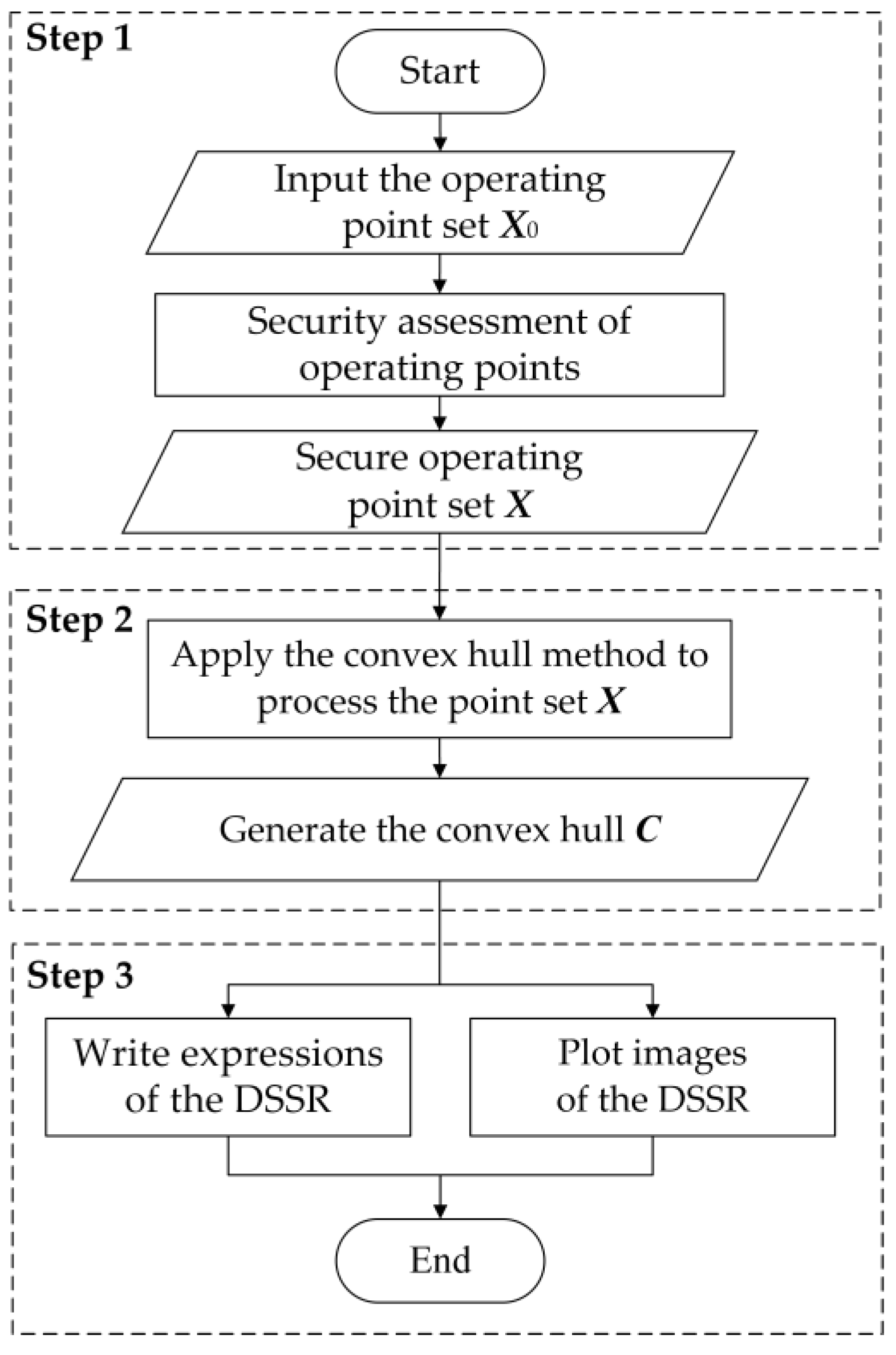
2.2. Convex Hull-Based Method for Solving the DSSR

2.2.1. Convex Set and Non-Convex Set

The concept of a convex set can be intuitively described as follows: a set is a convex set if the line segment that connects any two of its points lies entirely inside the set. The following mathematical definition [28] could also be used to characterize this.

In n-dimensional space, let x₁ and x₂ be two points in a set A. If the following condition (7) is met for all x₁, x₂ and λ (where λ is a real number and 0 ≤ λ ≤ 1), then A is a convex set:

$$\lambda {\mathit{x}}_1+\left(1-\lambda \right){\mathit{x}}_2\in \mathit{A}$$

(7)

Equation (7) is called a convex combination, which differs from normal linear combination in that λ can take any real value.

Otherwise, A is a non-convex set.

The property of the non-convex set can also be inferred from this definition. In a non-convex set, there must exist two points such that the line segment connecting them includes points not in the set.

2.2.2. Convex Hull Problem and Solving Algorithms

The convex hull problem [29] is a classical problem in computational geometry. The problem can be described as follows: given a set of points, construct a smallest convex set such that all given points are in or on the boundary of the convex set. This smallest convex set is referred to as the convex hull of the point set.

The algorithm for solving the convex hull problem takes a set of points as the input, then builds the convex hull boundary through methods such as sorting or divide-and-conquer, and finally outputs the desired convex hull [30]. Graham’s scan [31] and Quickhull algorithm [32] are commonly utilized algorithms. There are now comparatively mature tools for solving convex hull problems, such as the function “convhull” in Matlab, which can generate the convex hull by the Quickhull algorithm.

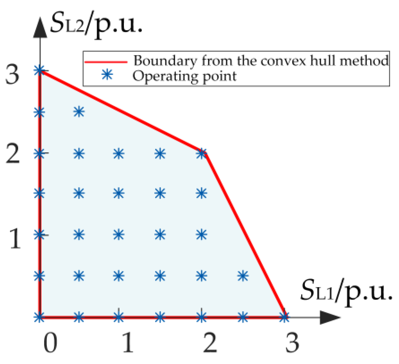
2.2.3. Convex Hull Method for Solving the DSSR

The secure operating points of a distribution network can form a set of points, while the DSSR is the set that encompasses all secure operating points. Therefore, the DSSR can be solved by the convex hull method with the input of secure operating point set. For the DSSR’s 2D or 3D observation of high-dimensional distribution systems, the power/load values of 2 or 3 components are selected as observation variables, while the power/load of all other components are frozen as constants. Thus, a series of 2D or 3D secure operating points are obtained. The specific steps of the convex hull based DSSR solving algorithm [19,20,21] are described below.

Step 1: Determine the set of secure boundary points based on security constraints. Secure boundary points are those operating points that are critical to secure. When a security constraint in Formula (4) changes from ”≤” to ”=”, that is, when g(W) = 0, the operating point W is considered a secure boundary point. Based on this property, methods such as uniform sampling, bisection approximation, or Monte Carlo sampling can be employed to obtain the secure boundary point set X:

$$\mathit{X}=\left\{\mathit{W}\in \mathsf{\Theta }\left|f(\mathit{W})=0, g(\mathit{W})=0\right.\right\}$$

(8)

Step 2: Apply the convex hull method to the secure boundary point set X. The algorithm sequentially selects and connects the vertices of X, while the remaining points are gradually deleted, thus the smallest convex set C containing all points of X is obtained as follows:

$$\mathit{C}=\left\{\mathit{W}={\displaystyle \sum _{i=1}^k{\lambda }_i{\mathit{W}}_i}\left|\mathit{W}\in \mathit{X}, {\lambda }_i\ge 0, {\displaystyle \sum _{i=1}^k{\lambda }_i}=1\right.\right\}$$

(9)

Step 3: Output the convex set C as the result of the DSSR. Provide analytical expressions of the DSSR derived from the convex hull. Then, observe the DSSR—draw the boundaries of DSSR and connect them to obtain the closed 2D or 3D image of DSSR.

The process of the convex hull method for solving the DSSR is shown in Figure 1.

3. Theoretical Analysis of Convex Hull Method for Solving the DSSR

3.1. Convex and Concave Regions of the DSSR

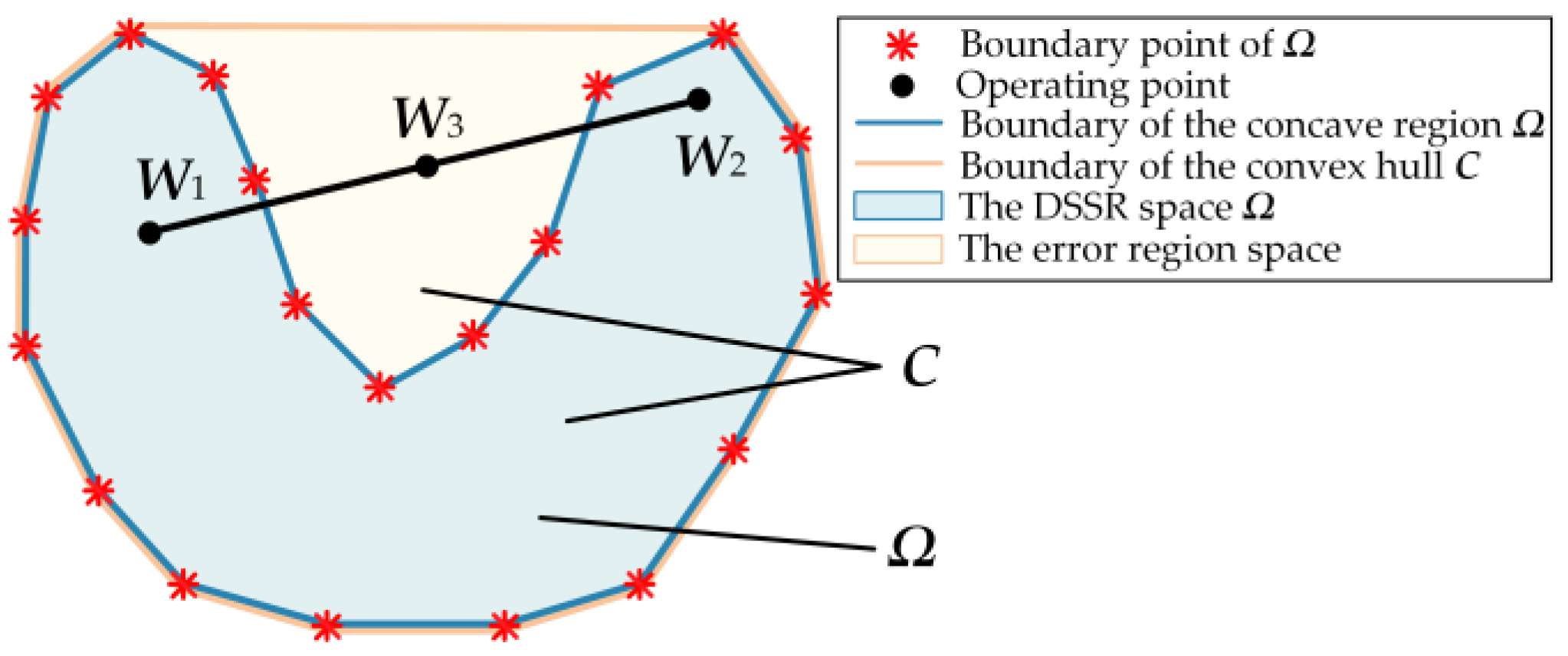
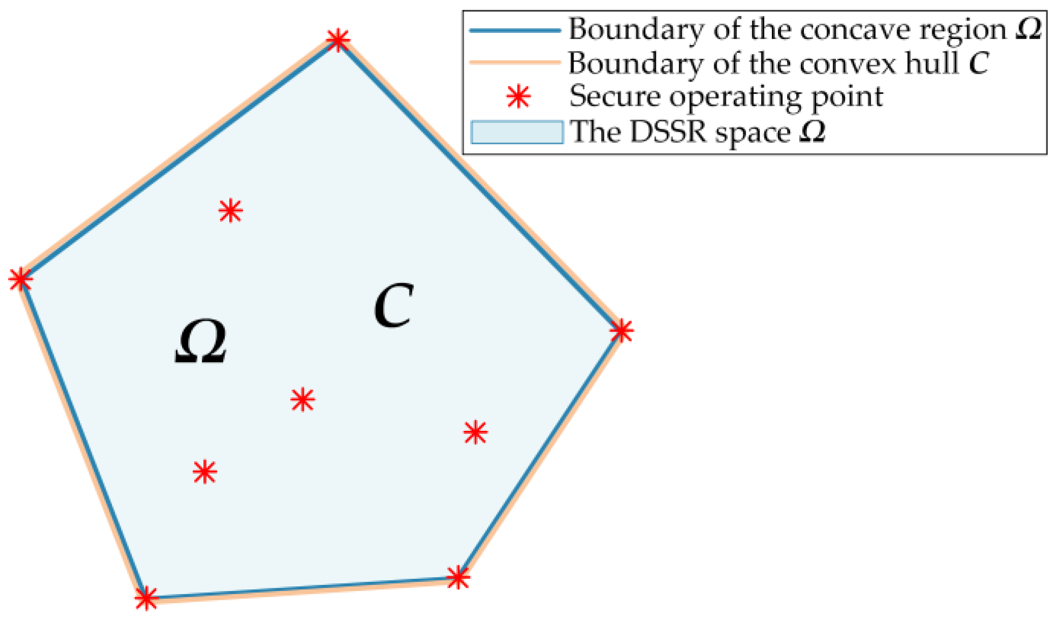
3.1.1. Concepts of the Convex Region and Concave Region

The DSSR exhibits characteristics of convexity and concavity: the secure operating point set of DSSR can be a convex set or a non-convex set. When a DSSR is a convex set, it is called a convex region; when a DSSR is a non-convex set, it is called a concave region [23].

The methods for determining convex and concave regions [24] are summarized as follows:

If a DSSR’s shape is a convex polyhedron, then it is a convex region.

If a DSSR’s shape is a concave polyhedron, then it is a concave region.

3.1.2. Formation Conditions for the Convex Region and Concave Region

The concavity and convexity of the DSSR are closely related to the number of load transfer schemes of the distribution network under N − 1 security criterion. The formation conditions of convex and concave regions [26] are as follows:

(1) If there is only one load transfer scheme (e.g., the N − 0 scenario, or the N − 1 scenario with single-backup or non-backup wirings) in a distribution system, a convex region will definitely be formed.

(2) If there are multiple load transfer schemes (e.g., the N − 1 scenario with multiple backup wirings) in a distribution system, a concave region will generally be formed. The only exception is a special case where the security region formed by one load transfer scheme covers all other regions, thus resulting in a convex region.

In real-world distribution networks, convex regions are mainly formed by single-backup or non-backup wirings, while concave regions are mainly formed by multiple backup wirings.

Multiple backup wirings are widely applied in practical distribution networks. Under the N − 1 security criterion, these distribution networks have multiple load transfer schemes, and concave regions of the DSSR are generally formed. Therefore, concave regions are widely present in real-world distribution networks.

3.2. Theorem and Proof of Error in the Convex Hull Method for Solving the Concave Region

Theorem 1. 

Error inevitably results when the convex hull method is applied to solve concave regions.

Proof of Theorem 1. 

Step 1: Examine the security of the convex combination of two operating points within a concave region.

Assume that there is a DSSR that is a concave region Ω, and that there exist two secure operating points W₁, W₂ ∈ Ω. A convex combination of the two points yields an operating point W₃, which satisfies the following:

$${\mathit{W}}_3=\lambda {\mathit{W}}_1+\left(1-\lambda \right){\mathit{W}}_2\notin \mathsf{\Omega }$$

(10)

λ is a real number in the interval [0,1].

W₃ is not in Ω. According to the definition of the DSSR, W₃ is an insecure operating point.

Step 2: Apply the convex hull method to the concave region Ω to obtain the convex hull C.

Input a series of points on the boundary of Ω, denoted as X = [x₁, x₂, …, x_n].

The output is the smallest convex set C that contains all points in Ω, such that

Ω ⊆ C

(11)

Step 3: Prove that W₃ is in the convex hull C.

From the definition of the convex set in Formula (7),

Since W₁, W₂ ∈ C,

$$\lambda {\mathit{W}}_1+\left(1-\lambda \right){\mathit{W}}_2\in \mathit{C}$$

(12)

Hence, W₃ ∈ C.

Therefore, there exists an operating point W₃ that is not in concave region Ω but is in the result C provided by the convex hull method.

The proof is complete. □

The relationship between the operating points and Ω and C is shown in Figure 2. It could be seen in Figure 2 that the insecure operating points in the indentation part of the state space are included in the solving result for the DSSR, forming an error region space in the convex hull method solution.

It could also be seen in Figure 2 that the space of security region obtained by the convex hull method is always larger than the precise result. If the convex hull method is applied to generate solutions for the DSSR, some insecure operating points would be misjudged as secure operating points, thus could not meet the requirements for security analysis of distribution networks.

Based on the proof of Theorem 1, this paper argues that the error generated by the convex hull method when solving concave regions is due to the nature of the method; thus, this type of error cannot be reduced or eliminated. Therefore, the convex hull method is not suitable for solving concave regions of the DSSR.

3.3. Theorem and Proof of Error in the Convex Hull Method for Solving the Convex Region

In addition to concave regions, this paper further discovers that the existing convex hull-based DSSR solving method [16,17,18] may also produce error when solving convex regions. In this section, the pertinent theorem and corollary are presented first, followed by the proof and error analysis.

Theorem 2. 

Error-free results can be reached when the convex hull method is applied to solve convex regions.

Corollary 1. 

The condition for reaching error-free results with the convex hull method for solving convex regions is that all vertices of the convex region are included in the input point set, and all other points inputted are secure operating points.

Proof of Theorem 2. 

Assume that there is a DSSR that is a convex region Ω, and the vertices are x₁, x₂, …, x_n. Apply the convex hull method to solve the DSSR.

Input the point set X:

X = [x₁, x₂, …, x_n, x_n+1, x_n+2, …, x_m]

(13)

where x_n+1, x_n+2, …, x_m are points inside Ω.

Select the vertices x₁, x₂, …, x_n by the convex hull method.

Generate the smallest convex set C that contains all these vertices.

Thus, both the convex region Ω and the convex hull method result C are convex hulls with vertices x₁, x₂, …, x_n.

The convex hull of a point set is uniquely determined [33]; so,

Ω = C

(14)

Therefore, the solution error of the convex hull method is zero.

The proof is complete. □

Theorem 2 and Corollary 1 are illustrated in Figure 3. It could be seen in Figure 3 that the result of convex hull method is completely identical to the accurate DSSR space, and there is no error that occurred in this case.

When the conditions in Corollary 1 are not met, error will be produced. The error is caused by two reasons, which are analyzed as follows:

Reason 1—Not all vertices of the convex region are included when determining the security boundary points. As the orange line shows in Figure 4a, this can cause the area of DSSR obtained by the convex hull method to be underestimated, and may lead to a reduction in the number of boundaries.

Reason 2—Some operating points outside the security region are misjudged as secure, resulting in the inclusion of these insecure points for input. As the orange line shows in Figure 4b, this can cause the area of the DSSR obtained by the convex hull method to be overestimated and may lead to an increase in the number of boundaries.

The error caused by the two reasons above can be reduced by decreasing the point-sampling interval or enhancing the accuracy of security assessment, until it reaches an error-free status. Therefore, the convex hull method is applicable to the solution of the convex region of the DSSR, provided that measures are taken to reduce the error.

3.4. Conditions for Distribution Networks Applying the Convex Hull Method

It is concluded that the convex hull method is suitable to solve convex regions but not concave regions, while both convex regions and concave regions universally exist in practical distribution systems [26]. The convexity and concavity of the DSSR [24] are closely related to the security criteria and distribution network structures. The applicability of the convex hull method is analyzed as follows:

(1) The convex hull method is suitable for all distribution networks’ N − 0 DSSR solutions. Since N − 0 means the security criterion under normal operation, there is no need to take load transfer schemes after N − 1 contingencies into consideration. Thus, N − 0 DSSRs are all convex regions, regardless of the network structures.

(2) For the N − 1 DSSR solutions, the convex hull method is only suitable for radial-structured networks and single-looped networks. Since there is only one load transfer path after an N − 1 contingency in these network structures [25], these DSSRs are convex regions that are suitable to apply the convex hull method. The method is not suitable for the multi-looped or meshed distribution networks’ N − 1 DSSR solutions. For multiple load transfer paths [25], these DSSRs are generally concave regions.

For network structures where the convex hull method is not applicable, the concave hull method is a potential extension to solve DSSRs, which will be a direction for future research.

4. Concave Region Case Study

The theoretical analysis in Section 2.2 reveals that the convex hull method inevitably generates error when solving concave regions. Here, a case study is conducted to demonstrate the error and to specifically analyze the adverse impacts caused by the error.

4.1. Overview of the Case

The distribution network shown in Figure 5 is a multi-backup wiring system called two-supply-one-backup wiring system. This is the simplest concave region distribution network example [22], which is widely used in South China urban areas.

The capacity of each feeder is 3 MVA. Each feeder is equipped with a normally closed feeder switch and a normally open tie switch so that each feeder could serve as a backup for other two feeders. Under N − 1 conditions, there are four load transfer schemes, namely, F₁ backup, F₂ backup, F₃ backup, and mutual backup. For example, F₁ backup means that F₁ serves as the backup for F₂ and F₃, with the potential load transfer paths being F₂ → F₁ and F₃ → F₁.

4.2. Solution of the DSSR

Select S_L1 and S_L2 as observation variables (S_Li refers to the load of feeder i), and the precise results of the N − 1 security region for this case can be obtained by the analytical method [13]. Here, the expressions of the security region and two-dimensional images are separately derived by the analytical method and convex hull method, and the results of the two methods are compared.

The “diagonal-bulge” and “diagonal-depression” scenarios are two earliest discovered and the most fundamental concave regions of the DSSR. The complex concave regions of larger distribution systems are also formed by these basic elements: diagonals, bulges, and depressions. Therefore, the two scenarios are separated in this case study.

4.2.1. Scenario 1: S_L3 = 1 MVA

(1)

Analytical method

The DSSR Ω of this scenario and its analytical expressions generated by the analytical method are as follows:

$$\mathsf{\Omega }=\left\{\mathit{W}\left|\begin{array}{l}{S}_{\mathrm{L}1}+S_{\mathrm{L}2}\le 3 \hspace{0.25em}\hspace{0.25em}\hspace{0.25em}\left(0\le S_{\mathrm{L}1}\le 1, 2\le S_{\mathrm{L}1}\le 3\right)\hfill \\ \begin{array}{l}{S}_{\mathrm{L}1}\le 2 \hspace{0.25em}\hspace{0.25em}\hspace{0.25em}\hspace{0.25em}\hspace{0.25em}\hspace{0.25em}\hspace{0.25em}\hspace{0.25em}\left(1\le S_{\mathrm{L}2}\le 2\right)\\ S_{\mathrm{L}2}\le 2 \hspace{0.25em}\hspace{0.25em}\hspace{0.25em}\hspace{0.25em}\hspace{0.25em}\hspace{0.25em}\hspace{0.25em}\hspace{0.25em}\left(1\le S_{\mathrm{L}1}\le 2\right)\\ S_{\mathrm{L}1}\ge 0 \hspace{0.25em}\hspace{0.25em}\hspace{0.25em}\hspace{0.25em}\hspace{0.25em}\hspace{0.25em}\hspace{0.25em}\hspace{0.25em}\left(0\le S_{\mathrm{L}2}\le 3\right)\\ S_{\mathrm{L}2}\ge 0 \hspace{0.25em}\hspace{0.25em}\hspace{0.25em}\hspace{0.25em}\hspace{0.25em}\hspace{0.25em}\hspace{0.25em}\hspace{0.25em}\left(0\le S_{\mathrm{L}1}\le 3\right)\end{array}\hfill \end{array}\right.\right\}$$

(15)

The image of the DSSR by the analytical method is the blue line shown in Figure 6a.

(2)

Convex hull method

Step 1: Input the secure operating points of the state space. In this scenario, the input points are O(0,0), A(0,3), B(1,2), C(2,2), D(2,1) and E(3,0).

Step 2: Apply the convex hull method to process the point set and to generate the convex hull.

Step 3: Output the convex hull C as a result, write the analytical expressions, and plot the image of the DSSR.

The DSSR C of this scenario and its analytical expressions generated by the convex hull method are as follows:

$$\mathit{C}=\left\{\mathit{W}\left|\begin{array}{l}0.5S_{\mathrm{L}1}+S_{\mathrm{L}2}\le 3 \hspace{0.25em}\hspace{0.25em}\hspace{0.25em}\left(0\le S_{\mathrm{L}1}\le 2\right)\hfill \\ \begin{array}{l}{S}_{\mathrm{L}1}+0.5S_{\mathrm{L}2}\le 3 \hspace{0.25em}\hspace{0.25em}\hspace{0.25em}\left(2\le S_{\mathrm{L}1}\le 3\right)\\ S_{\mathrm{L}1}\ge 0 \hspace{0.25em}\hspace{0.25em}\hspace{0.25em}\hspace{0.25em}\hspace{0.25em}\hspace{0.25em}\hspace{0.25em}\hspace{0.25em}\hspace{0.25em}\left(0\le S_{\mathrm{L}2}\le 3\right)\\ S_{\mathrm{L}2}\ge 0 \hspace{0.25em}\hspace{0.25em}\hspace{0.25em}\hspace{0.25em}\hspace{0.25em}\hspace{0.25em}\hspace{0.25em}\hspace{0.25em}\hspace{0.25em}\left(0\le S_{\mathrm{L}1}\le 3\right)\end{array}\hfill \end{array}\right.\right\}$$

(16)

The image of the DSSR by convex hull method is the red line shown in Figure 6a.

As can be seen in Figure 6a, the DSSR solution result of the convex hull method is larger than the precise result of the analytical method, with two extra triangular regions (△ABC and △CDE) added to the DSSR in this scenario.

4.2.2. Scenario 2: S_L3 = 2 MVA

(1)

Analytical method

The DSSR Ω of this scenario and its analytical expressions generated by the analytical method are as follows:

$$\mathsf{\Omega }=\left\{\mathit{W}\left|\begin{array}{l}{S}_{\mathrm{L}1}+S_{\mathrm{L}2}\le 3 \hspace{0.25em}\hspace{0.25em}\hspace{0.25em}\left(0\le S_{\mathrm{L}1}\le 1, 2\le S_{\mathrm{L}1}\le 3\right)\hfill \\ \begin{array}{l}{S}_{\mathrm{L}1}\le 1 \hspace{0.25em}\hspace{0.25em}\hspace{0.25em}\hspace{0.25em}\hspace{0.25em}\hspace{0.25em}\hspace{0.25em}\hspace{0.25em}\left(1\le S_{\mathrm{L}2}\le 2\right)\\ S_{\mathrm{L}2}\le 1 \hspace{0.25em}\hspace{0.25em}\hspace{0.25em}\hspace{0.25em}\hspace{0.25em}\hspace{0.25em}\hspace{0.25em}\hspace{0.25em}\left(1\le S_{\mathrm{L}1}\le 2\right)\\ S_{\mathrm{L}1}\ge 0 \hspace{0.25em}\hspace{0.25em}\hspace{0.25em}\hspace{0.25em}\hspace{0.25em}\hspace{0.25em}\hspace{0.25em}\hspace{0.25em}\left(0\le S_{\mathrm{L}2}\le 3\right)\\ S_{\mathrm{L}2}\ge 0 \hspace{0.25em}\hspace{0.25em}\hspace{0.25em}\hspace{0.25em}\hspace{0.25em}\hspace{0.25em}\hspace{0.25em}\hspace{0.25em}\left(0\le S_{\mathrm{L}1}\le 3\right)\end{array}\hfill \end{array}\right.\right\}$$

(17)

The image of the DSSR from the analytical method is the blue line shown in Figure 6b.

(2)

Convex hull method

The steps of the convex hull method are the same as those in Section 4.2.1. In this scenario, the input points are O(0,0), A(0,3), B(1,2), C(1,1), D(2,1) and E(3,0).

The DSSR C of this scenario and its analytical expressions generated by the convex hull method are as follows:

$$\mathit{C}=\left\{\mathit{W}\left|\begin{array}{l}{S}_{\mathrm{L}1}+S_{\mathrm{L}2}\le 3 \hspace{0.25em}\hspace{0.25em}\hspace{0.25em}\left(0\le S_{\mathrm{L}1}\le 3\right)\hfill \\ \begin{array}{l}{S}_{\mathrm{L}1}\ge 0 \hspace{0.25em}\hspace{0.25em}\hspace{0.25em}\hspace{0.25em}\hspace{0.25em}\hspace{0.25em}\hspace{0.25em}\hspace{0.25em}\hspace{0.25em}\left(0\le S_{\mathrm{L}2}\le 3\right)\\ S_{\mathrm{L}2}\ge 0 \hspace{0.25em}\hspace{0.25em}\hspace{0.25em}\hspace{0.25em}\hspace{0.25em}\hspace{0.25em}\hspace{0.25em}\hspace{0.25em}\hspace{0.25em}\left(0\le S_{\mathrm{L}1}\le 3\right)\end{array}\hfill \end{array}\right.\right\}$$

(18)

The image of the DSSR from the convex hull method is the red line shown in Figure 6b.

As can be seen in Figure 6b, the DSSR solution result of the convex hull method is also larger than the precise result of analytical method, with an extra right triangular region (△BCD) added to the DSSR of this scenario.

4.3. Error Analysis

The error of the convex hull method is analyzed from three aspects: the area of the DSSR, shape of the DSSR, and security analysis of the operating points.

4.3.1. Area of the DSSR

The area error of the convex hull method for the DSSR solution is shown in

Table 1. Area error of the convex hull method for the DSSR solution (concave region).

Scenario	Method	Area of the DSSR [MVA2]	Area Error [MVA2]	Relative Error [%]
Scenario 1	Analytical method	5	0	0
	Convex hull method	6	1	20
Scenario 2	Analytical method	4	0	0
	Convex hull method	4.5	0.5	12.5

.

As can be seen in Table 1, the convex hull method results in significant error in the area of DSSR, reaching up to 20% in the two scenarios.

The reason for the error is that the convex hull method misjudges the insecure regions in the indentation parts of the DSSR as secure, resulting in an overestimated security region area. This reason is consistent with the theoretical analysis in Section 3.2.

The extremum of the error is analyzed here by varying S_L3 to observe the error of convex hull method, with detailed information provided in Appendix A. The conclusions drawn are as follows:

(1)

When S_L3 is 0 or 1.5 MVA, the error is minimized at zero. The reason is that the DSSR is a convex region at these points.

(2)

When S_L3 is 3 MVA, the relative error is maximized at infinity. The reason is that the security region degenerates into an “L”-shaped polyline segment with zero area, while the convex set containing all points within the region is a triangle. Since the convex hull method still generates a nonzero area for this triangle, the relative error reaches infinity.

4.3.2. Shape of the DSSR

The shape of DSSR obtained by the convex hull method also exhibits deviations, as detailed in

Table 2. Shape error of the convex hull method for the DSSR solution (concave region).

Scenario	Method	Shape of the DSSR	Shape Deviation
Scenario 1	Analytical method	Non-convex hexagon OABCDE 1	None
	Convex hull method	Convex quadrilateral OACE 1	△ABC, △CDE 1
Scenario 2	Analytical method	Non-convex hexagon OABCDE 2	None
	Convex hull method	△OAE 2	△BCD 2

¹ In Figure 6a. ² In Figure 6b.

.

As can be seen in Table 2, the convex hull method inaccurately represents the shape of the DSSR, losing important information contained in the indentations of the DSSR image (e.g., line segments AB, AC, CD, and DE in scenario 1 and BC and CD in scenario 2).

Shape deviations also result in a reduction in the number of the DSSR boundaries compared with the actual situation.

4.3.3. Security Analysis of the Operating Points

The error of the convex hull method further leads to an incorrect security analysis. For example, the security analysis of some critical secure operating points is shown in

Table 3. Error of the operating point security analysis with the convex hull method.

Scenario	Method	Critical Secure Operating Points	Overlimit Power Flow [%]
Scenario 1	Analytical method	(1,2), (2,1)	0
	Convex hull method	(1.2,2.4), (2.4,1.2)	20
Scenario 2	Analytical method	(1,1)	0
	Convex hull method	(1.5,1.5)	50

.

As can be seen in Table 3, applying the DSSR result obtained by the convex hull method leads to serious misjudgments in the security analysis of operating points: among the operating points judged secure by the convex hull method, the maximum power flow overlimit reaches 1.5 times the allowed capacity limit. The reason is that the convex hull method does not consider the critical secure operating points in the indentations of the DSSR as security boundary points and assumes that the power flow of these operating points can still be increased, thus causing misjudgments in the security analysis. The misjudgments may further cause components to operate beyond their rated capacity, potentially leading to equipment overload, which can cause equipment failure or a reduced lifespan. They may also increase the duration of power outages and reduce system reliability.

It should be noted that the aforementioned errors in Section 4.3.1, Section 4.3.2 and Section 4.3.3 cannot be reduced by minimizing the point-sampling interval. Even if the precision is increased and more secure operating points in or on the boundaries of the DSSR are inputted, the error of the convex hull method will not be reduced. More details can be seen in Appendix B.

For larger distribution systems, DSSR solution errors will be produced by the convex hull method as well, and the errors will be even more severe because the degree of concavity is greater in complex distribution systems. Therefore, the convex hull method is not suitable for both simple and large-scale distribution systems whose DSSRs are concave regions.

5. Convex Region Case Study

The theoretical analysis in Section 3.3 reveals that error may also be produced by the convex hull method when solving convex regions. Here, a case study is conducted to verify this and further analyze the causes of the error, as well as to propose measures to reduce the error.

5.1. Overview of the Case

The active distribution network case with non-backup wiring is shown in Figure 7. The power limit of the two DGs is 0.4 MVA and of the two loads is 1.5 MVA.

A typical shape of the DSSR for this case is the convex pentagonal shape [12].

5.2. Solution of the DSSR

Select S_L1 and S_DG2 as observation variables, while S_DG1 and S_L2 are frozen at −0.4 MVA and 0.2 MVA. Apply the analytical method to obtain the DSSR Ω as follows:

$$\mathsf{\Omega }=\left\{\mathit{W}\left|\begin{array}{l}{S}_{\mathrm{L}1}+S_{\mathrm{DG}2}\le 0.8 \hspace{0.25em}\hspace{0.25em}\left(0.8\le S_{\mathrm{L}1}\le 1\right)\hfill \\ \begin{array}{l}{S}_{\mathrm{L}1}\le 1 \hspace{0.25em}\hspace{0.25em}\hspace{0.25em}\hspace{0.25em}\hspace{0.25em}\hspace{0.25em}\hspace{0.25em}\hspace{0.25em}\hspace{0.25em}\hspace{0.25em}\hspace{0.25em}\hspace{0.25em}\left(-0.2\le S_{\mathrm{DG}2}\le -0.4\right)\\ S_{\mathrm{DG}2}\le 0 \hspace{0.25em}\hspace{0.25em}\hspace{0.25em}\hspace{0.25em}\hspace{0.25em}\hspace{0.25em}\hspace{0.25em}\hspace{0.25em}\hspace{0.25em}\hspace{0.25em}\left(0\le S_{\mathrm{L}1}\le 0.8\right)\\ S_{\mathrm{L}1}\ge 0 \hspace{0.25em}\hspace{0.25em}\hspace{0.25em}\hspace{0.25em}\hspace{0.25em}\hspace{0.25em}\hspace{0.25em}\hspace{0.25em}\hspace{0.25em}\hspace{0.25em}\hspace{0.25em}\hspace{0.25em}\left(0\le S_{\mathrm{DG}2}\le -0.4\right)\\ S_{\mathrm{DG}2}\ge -0.4 \hspace{0.25em}\hspace{0.25em}\hspace{0.25em}\hspace{0.25em}\hspace{0.25em}\hspace{0.25em}\left(0\le S_{\mathrm{L}1}\le 1\right)\end{array}\hfill \end{array}\right.\right\}$$

(19)

In the convex hull method solution, the point-sampling interval is set to 0.2 MVA, resulting in 17 secure operating points. The DSSR C obtained is as follows:

$$\mathit{C}=\left\{\mathit{W}\left|\begin{array}{l}{S}_{\mathrm{L}1}+S_{\mathrm{DG}2}\le 0.85 \hspace{0.25em}\hspace{0.25em}\left(0.8\le S_{\mathrm{L}1}\le 1\right)\hfill \\ \begin{array}{l}{S}_{\mathrm{L}1}\le 1 \hspace{0.25em}\hspace{0.25em}\hspace{0.25em}\hspace{0.25em}\hspace{0.25em}\hspace{0.25em}\hspace{0.25em}\hspace{0.25em}\hspace{0.25em}\hspace{0.25em}\hspace{0.25em}\hspace{0.25em}\hspace{0.25em}\left(-0.15\le S_{\mathrm{DG}2}\le -0.35\right)\\ S_{\mathrm{DG}2}\le 0.05 \hspace{0.25em}\hspace{0.25em}\hspace{0.25em}\hspace{0.25em}\hspace{0.25em}\hspace{0.25em}\hspace{0.25em}\left(0\le S_{\mathrm{L}1}\le 0.8\right)\\ S_{\mathrm{L}1}\ge 0 \hspace{0.25em}\hspace{0.25em}\hspace{0.25em}\hspace{0.25em}\hspace{0.25em}\hspace{0.25em}\hspace{0.25em}\hspace{0.25em}\hspace{0.25em}\hspace{0.25em}\hspace{0.25em}\hspace{0.25em}\left(0.05\le S_{\mathrm{DG}2}\le -0.35\right)\\ S_{DG2}\ge -0.35 \hspace{0.25em}\hspace{0.25em}\hspace{0.25em}\hspace{0.25em}\hspace{0.25em}\hspace{0.25em}\left(0\le S_{\mathrm{L}1}\le 1\right)\end{array}\hfill \end{array}\right.\right\}$$

(20)

A visual comparison of the results obtained by the two methods is shown in Figure 8. As can be seen in Figure 8, the DSSR areas and shapes obtained by the two methods are the same, but the region space positions are different.

5.3. Error Analysis

The error of the convex hull method is analyzed below by combining the DSSR expressions and Figure 8.

5.3.1. Area of the DSSR

The area error of the DSSR obtained by the convex hull method in solving the convex region is shown in

Table 4. Area error of the convex hull method for the DSSR solution (convex region).

Method	Area of the DSSR [MVA2]	Area Error [MVA2]	Relative Error [%]
Analytical method	0.38	0	0
Convex hull method	0.38	0.1	13.2

.

As can be seen in Table 4, although the area of the DSSR obtained by the two methods is the same, there are areas in the upper and lower parts of the DSSR image given by the convex hull method that do not overlap with those in the analytical method. The areas of the upper and lower misaligned parts each account for 13.2% of the total area of the DSSR.

5.3.2. Shape of the DSSR

As shown in Figure 8, the shape of DSSR obtained by the two methods is the same. However, there is a displacement between the two results, causing the deviations in the positions of the upper and lower boundaries.

The different reasons for the deviations of the upper and lower boundaries are analyzed below.

The reason for the deviation in the lower boundary is that some vertices were not included, and instead, points inside DSSR (such as point B) were selected to be boundary points. The specific reason is that the point-sampling interval was large, resulting in an insufficient number of points being selected.

The reason for the deviation in the upper boundary is that there was a misjudgment in assessing of the security of operating points, leading to the inclusion of some insecure points (such as point A). The reasons for the misjudgment in security assessment are as follows:

(1)

The lenient convergence condition for the AC power flow model. For example, convergence condition in the case is

$$e=\left|S-S^{*}\right|<0.1 \mathrm{MVA}$$

(21)

(2)

The application of the DC power flow model.

5.3.3. Security Analysis of the Operating Points

The error of the DSSR solution by the convex hull method also leads to the incorrect security analysis of operating points, which is similar to that in concave hull case study, and so the detailed analysis is not elaborated here.

5.4. Error Reduction Measures

In response to the causes of error mentioned above, this paper proposes the following measures to reduce the error: minimizing the point-sampling interval to increase the number of input points and making the convergence condition stricter for the AC power flow model. Specifically, for this case study

(1)

The point-sampling interval is changed from 0.2 MVA to 0.05 MVA, increasing the number of input points from 17 to 179.

(2)

The convergence condition is modified to

$$e=\left|S-S^{*}\right|<0.02 \mathrm{MVA}$$

(22)

The DSSR image generated by the convex hull method with these measures taken is shown in Figure 9.

As can be seen in Figure 9, the result of the convex hull method completely overlaps with the accurate result, and the error is reduced to zero.

6. Conclusions

The solution of the distribution system security region (DSSR) is a fundamental issue, with the convex hull method used as a common approach. For the first time, this paper identifies the fact that the convex hull method can result in significant error when solving the DSSR. The study investigates this through both a theoretical analysis and case study validation. The primary works are as follows:

It is proven that the convex hull method will inevitably generate error when solving concave regions. The error stems from the inherent properties of the method and thus cannot be eliminated by taking simple measures. Case study validation reveals that when convex hull method is applied to solve concave regions, the area error is significant, important information of the DSSR’s geometric shape is lost, and this further leads to the misjudgment in the security analysis.

It is proven that the convex hull method can theoretically achieve error-free solutions for convex regions, and the conditions for achieving zero error are all vertices included and no insecure operating points included. Case study validation reveals that the convex hull method may also produce prominent error when solving practical convex regions. The reasons for the error are the large point-sampling interval and lenient convergence conditions, and measures to reduce the error are proposed. Attention should be paid when selecting the point-sampling interval and convergence conditions.

In practical use, when solving the N − 0 DSSR, the convex hull method is suitable for all distribution networks; but when solving the N − 1 DSSR, the method is only suitable for a radial-structured network and single-looped network.

This paper represents a vital revision of the fundamental theory of the DSSR. In the future, works should focus on the solution of concave regions by applying the concave hull method. For convex regions, further research should be conducted on the quantitative criteria for the point-sampling interval of the convex hull method to ensure that the error meets the engineering requirements.

References

1. Xiao, J.; Gu, W.; Wang, C.; Li, F. Distribution system security region: Definition, model and security assessment. IET Gener. Transm. Distrib. 2012, 6, 1029–1035. [Google Scholar] [CrossRef]
2. Saric, A.T.; Stankovic, A.M. Model uncertainty in security assessment of power systems. IEEE Trans. Power Syst. 2005, 20, 1398–1407. [Google Scholar] [CrossRef]
3. Kalyani, S.; Swarup, K.S. Particle swarm optimization based K-means clustering approach for security assessment in power systems. Expert Syst. Appl. 2011, 38, 10839–10846. [Google Scholar] [CrossRef]
4. Alimi, O.A.; Ouahada, K.; Abu-Mahfouz, A.M. A review of machine learning approaches to power system security and stability. IEEE Access 2020, 8, 113512–113531. [Google Scholar] [CrossRef]
5. Yang, T.; Yu, Y. Static voltage security region-based coordinated voltage control in smart distribution grids. IEEE Trans. Smart Grid 2017, 9, 5494–5502. [Google Scholar] [CrossRef]
6. Yang, T.; Yu, Y. Steady-state security region-based voltage/var optimization considering power injection uncertainties in distribution grids. IEEE Trans. Smart Grid 2018, 10, 2904–2911. [Google Scholar] [CrossRef]
7. Chen, S.; Chen, Q.; Xia, Q.; Kang, C. Steady-state security assessment method based on distance to security region boundaries. IET Gener. Transm. Distrib. 2013, 7, 288–297. [Google Scholar] [CrossRef]
8. Sun, B.; Li, Y.; Zeng, Y.; Chen, J.; Shi, J. Optimization planning method of distributed generation based on steady-state security region of distribution network. Energy Rep. 2022, 8, 4209–4222. [Google Scholar] [CrossRef]
9. Ding, T.; Bo, R.; Sun, H.; Li, F.; Guo, Q. A robust two-level coordinated static voltage security region for centrally integrated wind farms. IEEE Trans. Smart Grid 2015, 7, 460–470. [Google Scholar] [CrossRef]
10. Jiang, T.; Zhang, R.; Li, X.; Chen, H.; Li, G. Integrated energy system security region: Concepts, methods, and implementations. Appl. Energ. 2021, 283, 116124. [Google Scholar] [CrossRef]
11. Xiao, H.; Ye, Z.; Ma, F.; Ji, F. Calculation and analysis of the safe operation boundary of shipboard DC zonal electric distribution system. Trans. China Electr. Soc. 2016, 31, 202–208. [Google Scholar] [CrossRef]
12. Xiao, J.; Zu, G.; Zhou, H.; Zhang, X. Total quadrant security region for active distribution network with high penetration of distributed generation. J. Mod. Power Syst. Clean Energy 2021, 9, 128–137. [Google Scholar] [CrossRef]
13. Xiao, J.; Zhang, S.; Qiu, Z.; Song, C.; Jiao, H.; She, B. Geometric property of distribution system security region: Size and shape. Electr. Power Syst. Res. 2022, 210, 108106. [Google Scholar] [CrossRef]
14. Xiao, J.; Song, C.; Jiao, H.; Li, Z.; Li, J.; Li, C. Stability modeling and solution for security region of integrated energy system based on energy circuit. Autom. Electr. Power Syst. 2023, 47, 53–63. [Google Scholar] [CrossRef]
15. Song, C.; Xiao, J.; Qiu, Z.; Jiao, H.; Qu, Y. Steady state model of security region for natural gas network based on unified modeling method of heterogeneous energy. Autom. Electr. Power Syst. 2022, 46, 13–22. [Google Scholar] [CrossRef]
16. Huang, Z.; Wu, Z.; Yan, H. A convex-hull based method with manifold projections for detecting cell protrusions. Comput. Biol. Med. 2024, 173, 108350. [Google Scholar] [CrossRef]
17. Yi, K.; Sun, L.; Ding, J.; Ding, M. Load restoration scheme optimization for power system with wind power based on convex hull theory. Autom. Electr. Power Syst. 2024, 48, 77–87. [Google Scholar] [CrossRef]
18. Lei, C.; Bu, S.; Zhong, J.; Chen, Q.; Wang, Q. Distribution network reconfiguration: A disjunctive convex hull approach. IEEE Trans. Power Syst. 2023, 38, 5926–5929. [Google Scholar] [CrossRef]
19. Pei, L.; Wei, Z.; Chen, S.; Sun, G.; Lyu, S. Convex hull based security region for AC/DC hybrid distribution networks. Autom. Electr. Power Syst. 2021, 45, 45–51. [Google Scholar] [CrossRef]
20. Pei, L.; Wei, Z.; Chen, S.; Zhao, J.; Yin, H. Security region of variable photovoltaic generation in AC-DC hybrid distribution power networks. Power Syst. Technol. 2021, 45, 4084–4093. [Google Scholar] [CrossRef]
21. Chen, S.; Wei, Z.; Sun, G.; Wei, W.; Wang, D. Convex hull based robust security region for electricity-gas integrated energy systems. IEEE Trans. Power Syst. 2018, 34, 1740–1748. [Google Scholar] [CrossRef]
22. Xiao, J.; Jiao, H.; Qu, Y.; She, B. Special two-dimensional images of distribution system security region: Discovery, Mechanism and Application. Proc. CSEE 2020, 40, 5088–5102. [Google Scholar] [CrossRef]
23. Xiao, J.; Jiao, H.; Song, C.; Qiu, Z.; Bao, Z. New Images of Map for Distribution System Security Region. In Proceedings of the 2022 IEEE Power & Energy Society General Meeting (PESGM), Denver, CO, USA, 17–21 July 2022; pp. 1–5. [Google Scholar] [CrossRef]
24. Xiao, J.; Cao, Y.; Zhang, B. Concavity and convexity of distribution system security region: Theorem, Proof and Determination Algorithm. Proc. CSEE 2021, 41, 5153–5167. [Google Scholar] [CrossRef]
25. Jiao, H.; Lin, X.; Xiao, J.; Zu, G.; Song, C.; Qiu, Z.; Bao, Z.; Zhou, C. Concavity-convexity of distribution system security region. Part I: Observation results and mechanism. Appl. Energ. 2023, 342, 121169. [Google Scholar] [CrossRef]
26. Jiao, H.; Xiao, J.; Zu, G.; Song, C.; Lv, Z.; Bao, Z.; Qiu, Z. Concavity-convexity of distribution system security region. Part II: Mathematical principle, judgment, and application. Appl. Energ. 2024, 361, 122888. [Google Scholar] [CrossRef]
27. Xiao, J.; Wang, C.; She, B.; Li, F.; Bao, Z.; Zhang, X. Total supply and accommodation capability curves for active distribution networks: Concept and model. Int. J. Elec. Power 2021, 133, 107279. [Google Scholar] [CrossRef]
28. Niestegge, G. Quantum transition probability in convex sets and self-dual cones. Proc. R. Soc. A 2024, 480, 20230941. [Google Scholar] [CrossRef]
29. Wei, L.; Atamtürk, A.; Gómez, A.; Küçükyavuz, S. On the convex hull of convex quadratic optimization problems with indicators. Math. Program. 2024, 204, 703–737. [Google Scholar] [CrossRef]
30. Gamby, A.N.; Katajainen, J. Convex-hull algorithms: Implementation, testing, and experimentation. Algorithms 2018, 11, 195. [Google Scholar] [CrossRef]
31. Sivakumar, V.L.; Ramkumar, K.; Vidhya, K.; Gobinathan, B.; Gietahun, Y.W. A comparative analysis of methods of endmember selection for use in subpixel classification: A convex hull approach. Comput. Intel. Neurosc. 2022, 2022, 3770871. [Google Scholar] [CrossRef]
32. Alshamrani, R.; Alshehri, F.; Kurdi, H. A preprocessing technique for fast convex hull computation. Procedia Comput. Sci. 2020, 170, 317–324. [Google Scholar] [CrossRef]
33. Kwon, H.; Oh, S.; Baek, J.W. Algorithmic efficiency in convex hull computation: Insights from 2d and 3d implementations. Symmetry 2024, 16, 1590. [Google Scholar] [CrossRef]
Figure 1. Flow chart of the convex hull method for solving the DSSR.
Energies 18 02327 g001
Figure 2. Illustration of the error proof for the convex hull method.
Energies 18 02327 g002
Figure 3. The condition for the error-free convex region solution of the convex hull method.
Energies 18 02327 g003
Figure 4. Causes of the error in the convex hull method for the convex region solution. (a) Error cause 1: not all vertices are included. (b) Error cause 2: insecure operating points are included.
Energies 18 02327 g004
Figure 5. Case of the two-supply-one-backup wiring system.
Energies 18 02327 g005
Figure 6. Comparison of DSSR solutions between the analytical method and convex hull method. (a) Concave region scenario 1; (b) concave region scenario 2.
Energies 18 02327 g006
Figure 7. Case of the 4-node active distribution network (non-backup wiring).
Energies 18 02327 g007
Figure 8. Comparison of DSSR solutions between the analytical method and convex hull method (convex region).
Energies 18 02327 g008
Figure 9. DSSR solution by the convex hull method after measures were taken to reduce error.
Energies 18 02327 g009