1. Introduction
The global energy landscape has witnessed unprecedented growth in renewable energy penetration, with solar photovoltaic capacity reaching over 1.6 TW globally by 2023, representing more than a ten-fold increase from 2010 levels. In recent years, there has been a remarkable surge in the penetration of renewable energy sources, particularly wind and solar power, driven by environmental conservation and energy efficiency initiatives. In a power system, distributed solar generation, primarily implemented through rooftop photovoltaic installations, has demonstrated steady growth. This expansion is attributed to several advantages: close proximity to load centers, minimal spatial requirements, and reduced transmission losses.
However, field studies from multiple grid operators worldwide have documented significant technical challenges arising from high PV penetration. Due to the relatively high conductor impedance of distribution networks, the node voltages are particularly susceptible to active power variations. This sensitivity becomes increasingly problematic as the penetration rate of PV systems escalates within distribution networks, with utilities reporting overvoltage incidents affecting up to 50% of end-users in high-penetration scenarios. The intermittent nature of solar power generation introduces significant fluctuations in nodal active power injection, leading to voltage instability and, in some cases, overvoltage at the nodes. These technical challenges not only compromise the power system’s operational efficiency through increased power losses but also pose substantial risks to grid stability and reliability [
1,
2,
3].
In power systems, reactive power management has emerged as a fundamental approach for effective voltage regulation [
4,
5,
6]. Conventional voltage regulation methods, such as step voltage regulators (SVRs), on-load tap changers (OLTCs), and capacitor banks, have served as primary longer-term voltage control mechanisms. However, these devices not only incur significant capital expenditure but also face mechanical limitations that restrict their application in scenarios requiring frequent switching operations [
7,
8,
9]. In contrast, PV inverters offer superior reactive power control capabilities with rapid response and continuous adjustment ranges. By utilizing the available reactive power capacity of PV inverters, substantial cost reductions in reactive power infrastructure investments can be achieved [
10]. This approach enables real-time voltage regulation during transient conditions and effectively mitigates overvoltage scenarios, thereby maintaining the power network within optimal operational parameters [
11]. The integration of inverter-based reactive power control not only enhances system flexibility but also promotes a more resilient and efficient operation.
Voltage regulation methods employing distributed energy sources can be categorized into three approaches, each with specific limitations that constrain their practical implementation. The first category relies on local measurements from distributed energy sources to modulate their power output for voltage regulation. Conventional droop control, as described by Neal et al. in [
10,
11,
12], is the predominant local voltage regulation approach.
This method modulates reactive power output to regulate nodal voltage based on a predefined reactive power–voltage characteristic curve. However, as demonstrated by Li et al. [
13], traditional droop control may fail to maintain voltage stability under certain operating conditions. Guo et al. [
14] presents an enhanced droop control framework utilizing gradient projection; however, its effectiveness is constrained by fixed reactive power–voltage slopes. In [
15], Cheng et al. introduced an adaptive local voltage control strategy, where each bus agent can dynamically adapt its voltage droop function in response to temporal system variations, enhancing reactive power–voltage control flexibility. Zhang et al. [
16] proposed a sensitivity-based mixed coordination algorithm. However, to ensure that the voltage of all buses within the region stay within the limits, multiple iterations are required. In each iteration, the bus with the largest voltage deviation is selected through voltage estimation, and a global sensitivity calculation is performed to choose the appropriate reactive power injection for the node until no bus exceeds the voltage limit. This process demands significant computational resources and has a relatively slow convergence speed. Although these approaches eliminate communication network dependencies, they may prove insufficient for rapid and comprehensive voltage regulation across the power network.
The second method category for voltage regulation is characterized by systematic data collection and centralized optimization computations. In [
17], Tang et al. developed a centralized optimization algorithm leveraging the quasi-Newton method with second-order differential data, enabling real-time optimal power flow monitoring. Dall’ Anese et al. [
18] employ real-time measurement-based optimal power flow computations through a dual ε-sub gradient algorithm, employing convex relaxation techniques to address optimization non-convexity. Dall’Anese and Simonetto [
19] utilize real-time data for optimal power flow calculations through linear power flow approximations and Lagrangian regularization. Khunkitti et al. [
20] introduce the Harris hawks optimization (HHO) algorithm, which models the cooperative hunting behavior of Harris hawks through exploration, transition, and exploitation phases.
The third category involves distributed control strategies utilizing smart terminals at network nodes, combining local measurements with inter-node communication. This approach facilitates collaborative computation while minimizing communication infrastructure requirements, offering a cost-effective solution. In [
21], Qu and Li employed a distributed method based on dual decomposition to address the optimal reactive power flow problem in distribution networks, though it requires comprehensive nodal measurement. While Chang et al. [
22] introduce an innovative dual ascent algorithm requiring only partial nodal measurements and local communication, it maintains the centralized processing of Lagrange multipliers. The algorithm proposed by Bolognani et al. [
23] only necessitates voltage amplitude and phase angle measurements from distributed energy source nodes, enabling optimization through neighbor-to-neighbor communication. However, the requirement for synchronized phase measurements presents significant implementation challenges and may not guarantee voltage regulation at load nodes.
Zheng et al. [
24,
25] implement a distributed approach using the Alternating Direction Method of Multipliers (ADMMs), incorporating both upper-level variable exchange and lower-level local optimization processes. Sadnan and Dubey [
26] present a hybrid methodology combining primal decomposition with block coordinate descent for distributed reactive power optimization, though these approaches demand substantial computational resources at each agent node.
Current distributed methods either require extensive measurement infrastructure, suffer from convergence issues in poorly conditioned networks, or cannot guarantee voltage regulation across all network nodes without sophisticated communication protocols.
The literature review reveals a critical gap in developing practical distributed optimization methods that balance computational efficiency, communication requirements, and voltage regulation effectiveness for medium-voltage distribution networks with high PV penetration. Existing approaches demonstrate limitations in scalability, measurement requirements, or convergence reliability that restrict their practical deployment.
This paper presents a novel distributed optimization methodology for reactive power–voltage control specifically designed for medium-voltage distribution networks with high photovoltaic penetration. The primary objective focuses on power loss minimization, utilizing limited measurement data from distributed photovoltaic nodes and critical locations, supplemented by inter-node communication. Based on information exchange, the method iteratively resolves the optimal reactive power flow problem through straightforward calculations.
The contributions of this research include the following:
Development of an efficient network loss model utilizing selective nodal measurements of voltage and line power, addressing practical distribution network constraints.
Implementation of a comprehensive strategy that effectively mitigates voltage violations while optimizing network losses, enhancing both the economic efficiency and operational safety of distribution networks.
Integration of an adaptive step size algorithm that eliminates manual parameter tuning requirements, promoting the efficiency of reactive power–voltage optimization control.
The remainder of this paper is organized as follows.
Section 2 presents the reactive power–voltage optimization model.
Section 3 details the proposed voltage control methodology.
Section 4 provides a comprehensive case study analysis, and
Section 5 concludes this paper by summarizing key findings, implications, and directions for future work.
2. Reactive Power–Voltage Optimization Model
This paper addresses the enhancement of a distribution network’s safety and economic operation. The approach minimizes network losses while maintaining voltage stability through the coordinated reactive power control of distributed photovoltaic inverters operating under PQ control schemes. Given the sub-second temporal requirements of this control problem, traditional reactive power compensation devices and on-load tap changers are excluded from consideration due to their inherently slow response characteristics.
In detailed distribution network models, the relationships between nodal voltages, network losses, and reactive power injection from distributed energy resources manifest as complex nonlinear functions. The real-time optimization of these interconnected parameters presents significant computational challenges, particularly within distributed control architectures. Therefore, developing appropriate network model approximations is essential for implementing practical distributed reactive power optimization strategies.
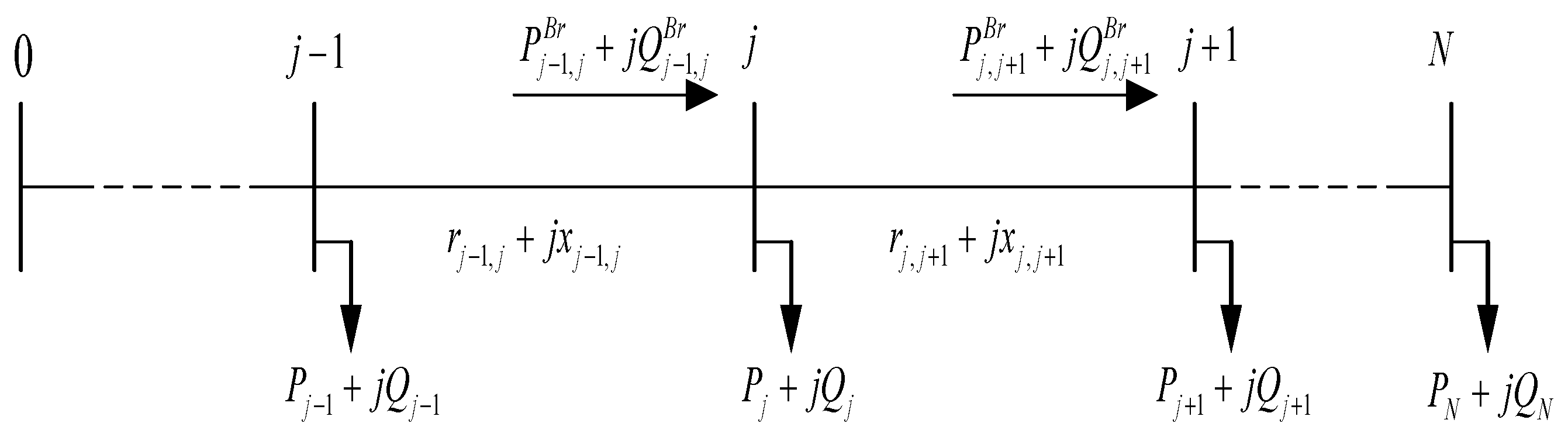
Consider a single-line network consisting of N + 1 nodes, as illustrated in
Figure 1. The branch currents are expressed by Equations (1)–(3) in [
27]:
In this formulation, the power flow parameters are defined as follows: Pj and Qj denote the active and reactive powers flowing out of node j. Vj denotes the voltage magnitude at node j, while rj and xj correspond to the equivalent resistance and reactance of branch j, respectively.
This paper adopts the linear power flow model in [
28], which provides approximation via the following linear model, where
Ploss represents the aggregate power losses in the distribution network:
Power injection from nodes into lines is defined as positive power. The power flow directed towards the root node is established as the positive direction, while the voltage magnitude at the root node is normalized such that
V0 = 1. Under these conventions, applying Equations (4)–(6) to a radial network structure yields the following mathematical relationships in Equations (8)–(11):
By combining Equations (8)–(11), Equation (12) can be derived.
PBr and
QBr denote vectors encompassing active power and reactive power flowing through each branch, respectively.
VBr constitutes a vector comprising voltage drops across each branch, while
V is a vector encompassing voltage magnitudes at various nodes.
diag(r) and
diag(x) represent diagonal matrices derived from the equivalent resistance and reactance of each branch, respectively. The matrix
A characterizes the network’s topology, with its element in the
i-th row and
j-th column illustrating the relationship between node
i and node
j, as demonstrated in Equation (13), where
e0,j signifies the path from node
j to the root node.
The node variables are divided into two types, nodes that contain distributed energy sources and nodes that do not, and they are as follows:
In Equation (14), VG and VL represent the voltage magnitudes of nodes with and without distributed energy sources, respectively. PG, PLG, and PL are the active power output of distributed energy sources, the active power absorbed by loads in nodes with distributed energy sources, and the active power absorbed by loads in nodes without distributed energy sources, respectively. Similarly, QG, QLG, and QL signify the reactive power output of distributed energy sources, the reactive power absorbed by loads in nodes with distributed energy sources, and the reactive power absorbed by loads in nodes without distributed energy sources, respectively. The matrices are formulated as ATdiag(r)A, ATdiag(x)A, respectively.
The block matrices MR and MX have dimensions g × g, where g represents the number of nodes with distributed energy sources. NR and NX have dimensions g × (N − g), and UR and UX have dimensions (N − g) × (N − g), where N denotes the total number of nodes (excluding the reference or balancing node).
For distribution networks, obtaining measurements from all nodes presents significant technical challenges. Therefore, installing measurement devices at nodes containing distributed photovoltaic sources becomes crucial for system monitoring and control.
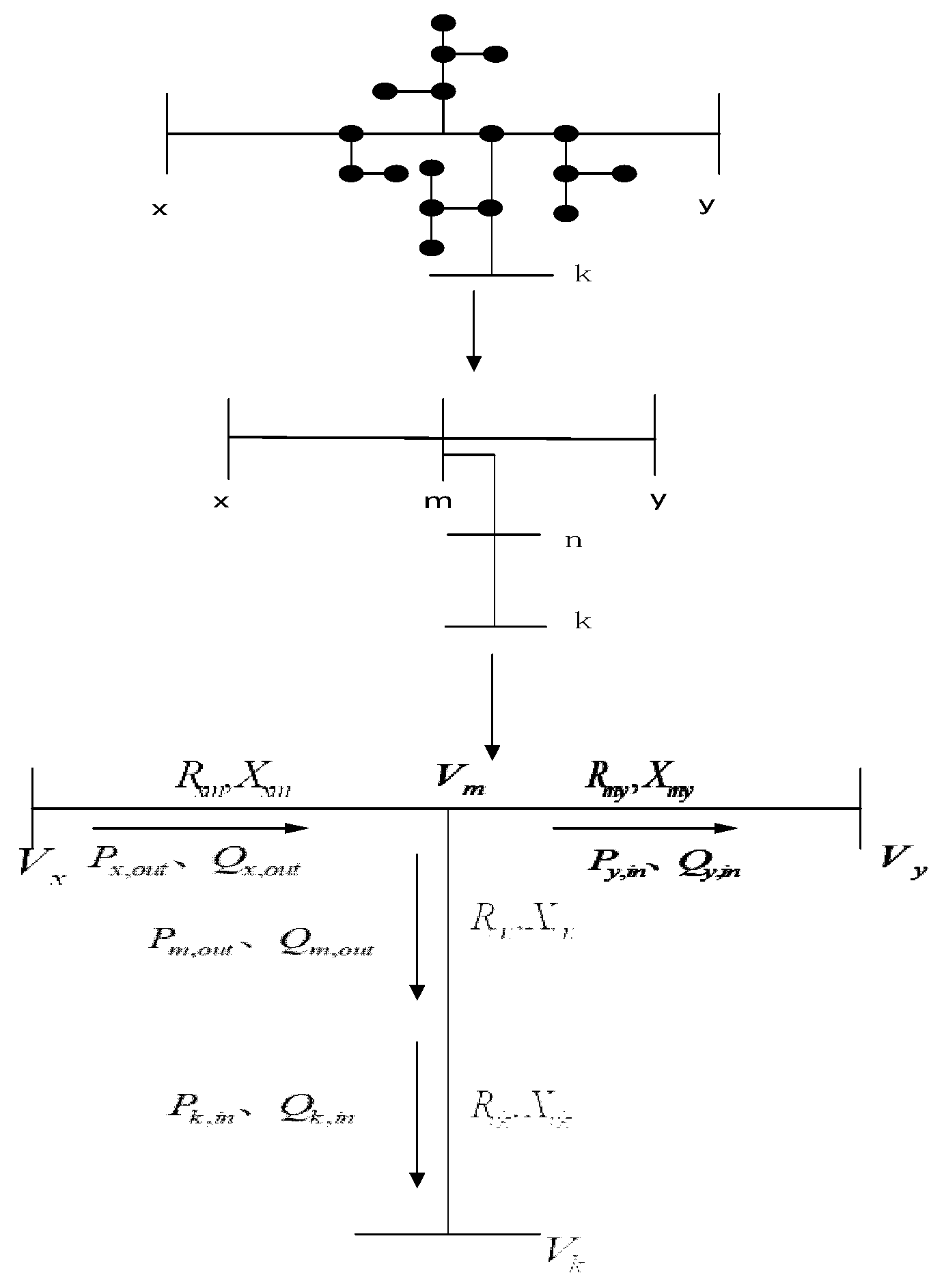
In scenario 1, as shown in
Figure 2, the process involves simplifying the network between two measurable nodes, designated as
x and
y.
Px,out and
Qx,out represent the outgoing active power and reactive power at node
x, while
Py,in and
Qy,in represent the incoming active power and reactive power at node
y.
Pz,in and
Qz,in indicate the active power and reactive power flowing into the virtual node
z. The parameters
Rxz and
Xxz describe the equivalent resistance and reactance of the line between nodes
x and
z, while
Rzy and
Xzy characterize the equivalent resistance and reactance between nodes
y and
z.
Based on the power flow model and assuming negligible line losses, Equation (15) can be derived as follows:
In this simplified model, the line impedance constraints are expressed by Equations (16) and (17):
For cases where the impedance of the line segments is not significantly different, the approximation takes the following form:
Consequently, the network losses between nodes x and y can be equivalently expressed by Equation (19).
Scenario 2, as depicted in
Figure 3, presents a network simplification approach for configurations where a T-node exists between adjacent measurement nodes, with additional measurement nodes present on the T-node branches. The power flows in this configuration are defined as follows:
Px,out and
Qx,out represent the outgoing active and reactive power from node
x, while
Py,in,
Pk,in,
Qy,in, and
Qk,in denote the incoming active and reactive power at nodes
y and
k. Additionally,
Pm,out and
Qm,out characterize the outgoing active and reactive power from the virtual node m.
The electrical parameters in this configuration are defined as follows: Rxm and Xxm represent the equivalent resistance and reactance of the connection between nodes x and m, while Rmy and Xmy represent the equivalent resistance and reactance of the link between node y and m. Further, Rkn, Rmn, Xkn, and Xmn are the equivalent resistance and reactance of the connections involving nodes k, m, and virtual node n.
Following the previously established equivalent model, the relationship can be expressed as follows:
Hence, the power losses between nodes
x,
y, and
k can be represented by Equation (21).
Therefore, the distribution network losses
Ploss can be represented by Equation (22):
In scenario 1, the set CM1 represents measurement nodes, where ‘x: x→y’ indicates measurement node ‘x’ upstream of node ‘y’, and ‘z: x→z→y’ indicates virtual node ‘z’ between measurement nodes ‘x’ and ‘y’. Virtual nodes ‘m’ and ‘n’, depicted as ‘n: x→m→n→k’, are positioned between measurement nodes ‘x’ and ‘k’.
In scenario 2, CM2 represents the set of measurement nodes, with ‘x: x→y’ and ‘x: x→k’ indicating that measurement node ‘x’ supplies data to downstream nodes ‘y’ and ‘k’. The virtual node ‘m’ is interposed between measurement nodes ‘x’ and ‘y’, as indicated by ‘m: x→m→y’. Additionally, for virtual nodes, ‘m’ and ‘n’ between measurement nodes ‘x’ and ‘k’ are denoted as ‘n: x→m→n→k’.
3. Voltage Control Methodology
For the secure operation of the distribution network, it is imperative that the voltages at different nodes remain within the specified voltage safety range. If the set of distribution network nodes is denoted as NP, this constraint can be expressed as Equation (23):
Equations (24) and (25) represent the operational constraints for distributed PVs.
Here, QGi and SGi, respectively, represent the reactive power output and rated capacity of the i-th photovoltaic unit, while NG is the set of nodes where distributed photovoltaics are located.
Hence, the problem of optimizing reactive power can be formulated as Equation (26):
3.1. Voltage Estimation
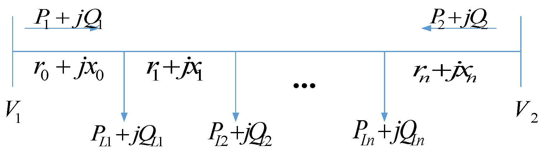
In distribution networks where comprehensive node measurements are unavailable, voltage estimation becomes necessary at nodes without measurement devices. This estimation is particularly crucial for determining the minimum node voltage, which serves as a key parameter for reactive power-based voltage control. The voltage estimation algorithm assumes uniform load distributions between measurement nodes, and it proceeds as follows.
Figure 4 depicts
n pure load nodes between two measurement nodes, labeled as 1 and 2. The power flows at these measurement nodes are expressed as
P1 + jQ1 and
P2 + jQ2, respectively. Under the uniform load assumption, each node carries an average load of
PL + jQL, which can be calculated using Equations (27) and (28).
If P1 > 0, P2 < 0, Q1 > 0, and Q2 < 0, the minimum voltage is located at measurement node 2. Conversely, when P2 > 0, P1 < 0, Q2 > 0, and Q1 < 0, the minimum voltage is situated at measurement node 1.
The estimation of minimum voltage for all remaining scenarios is given by Equation (29), where
Vmin represents the estimated minimum voltage along the line. The “
ceil” function rounds up to the nearest integer, with a lower bound of 0.
Based on the estimated minimum voltage, the lower voltage limits for the two measurement nodes can be adjusted according to Equation (30).
For configurations involving three measurement nodes, the minimum node voltage estimation proceeds under the assumption of uniform load distribution between measurement nodes. The estimation algorithm is structured as follows.
Figure 5 illustrates the presence of
n load-only nodes situated between three measurement nodes: 1, 2, and 3. The power discharged from these measurement nodes is represented as
P1 + jQ1,
P2 + jQ2, and
P3 + jQ3. Additionally, the average load per node is denoted as
PL + jQL, with its calculation formula provided in Equations (31) and (32).
When P1 > 0, P2 < 0, P3 > 0, and Q1 > 0, Q2 < 0, Q3 > 0, the minimum voltage is at measurement node 2. When P1 > 0, P2 > 0, P3 < 0, and Q1 > 0, Q2 > 0, Q3 < 0, the minimum voltage is at measurement node 3. When P1 < 0, P2 > 0, P3 > 0, and Q1 < 0, Q2 > 0, Q3 > 0, the minimum voltage is at measurement node 1.
In all other cases, the formula for estimating the minimum voltage is shown in Equations (33) and (34):
where
n1,
n2, and
n3 represent the number of purely load nodes between the three measurement nodes and the T-node. The minimum voltage thresholds for the three measurement nodes are determined based on Formula (30).
3.2. Improved Dynamic Projection Dual Distributed Optimization Algorithm
Distributed optimization solves optimization problems through a decentralized approach, utilizing local computations and communications, without requiring access to global information. Within this framework, agents possess both communication and computational capabilities. On the other hand, multi-agent systems are networks composed of multiple agents that collaborate and communicate to attain a common objective. Within a multi-agent system, each agent processes its locally available information, and it interacts based on predefined protocols, working collectively to achieve specific goals. This distributed architecture enables each agent to operate using only local data while coordinating with other agents to achieve global optimization objectives.
For a network of
N agents, the objective is to solve a distributed optimization problem with inequality constraints. Each agent maintains its own objective function and constraints. The comprehensive optimization problem is formulated as Equation (35):
In Equation (35), X represents the solution vector, and fi denotes the local objective function for agent i, yielding real number values. gi represents the local inequality constraint function for agent i. For the i-th agent with pi inequality constraints, gi = (gi1, gi2,…, gipi)T. is a closed convex set of real numbers, and both fi and gi are convex functions.
Building upon the reactive power optimization problem in Equation (26), this paper generalizes the approach to Equation (35). Recognizing the practical challenges of agents with limited state-sensing capabilities, this study introduces an enhanced dynamic projection dual distributed optimization algorithm, extending the work of reference [
27]. The agents capable of sensing their local states can adjust their solution vectors based on local information and communication, whereas agents without sensing capabilities update their solution vectors through communication alone. Let
Na denote the set of agents capable of sensing their local states, and let
Nb denote the set of agents unable to sense their local states. The refined dynamic projection dual distributed algorithm is characterized by Equations (36) and (37), with convergence proof provided in
Appendix A. The proven convergence properties ensure that the algorithm’s performance will remain consistent when applied to larger systems, as the underlying optimization principles remain invariant to scale.
Here, signifies the projection of vector onto the tangent cone , which is represented as .
Consider
X as the solution vector consisting of
n elements, and for agent
i, the solution vector is denoted as
Xi = (xi,1, xi,2,…, xi,n)T. The relevant mathematical expressions are elaborated as follows:
Here, aij represents the communication relationship between nodes i and j. If there is no communication channel between nodes i and j or when i = j, aij = 0; otherwise, aij = 1. The operator (x)+ is defined as follows: if x ˃ 0, (x)+ = x; if x ≤ 0, (x)+ = 0.
3.3. Distribution Network Reactive Power–Voltage Optimization Control Method
This active distribution network encompasses
g nodes with distributed PV and
l load-only nodes. The PV-integrated nodes are capable of measuring their voltage magnitude, as well as the active and reactive power transmitted through their connected lines. When the topology between PV-integrated nodes deviates from the reference configurations presented in
Figure 4 or
Figure 5 of
Section 3.1, the strategic placement of additional measurement devices at select load-only nodes becomes necessary. These supplementary measurement points must replicate the capabilities of PV-integrated nodes to establish the desired topological relationships outlined in the aforementioned figures. Furthermore, cost-effective voltage magnitude sensors can be affixed at the terminal nodes, while the remaining load-only nodes operate without measurement capabilities.
For scenarios involving a measurable node with multiple downstream branches lacking intermediate measurable points, the aggregate network losses for all downstream nodes are approximated by the line losses between the measurable node and its immediate downstream connections. The computation of the network loss is distributed across the system, with each measurable node performing its portion of the computational load. Assuming a measurable node
x located between upstream virtual node
z1 and downstream virtual node
z2, the calculation of network loss by the measurable node
x follows Equation (40).
The global network loss (
Ploss) is decomposed into constituent components through a distributed computational framework, where each measurable node
x contributes its locally calculated loss value (
Ploss,x). This decomposition is mathematically formulated in Equation (41), with
CM representing the comprehensive set of measurable nodes.
Within the distribution network topology, a subset of
g nodes is integrated with PV systems. The
j-th PV-integrated node is denoted as
gj, where
j ranges from 1 to
g (
j =
1, 2,…, g). The reactive power output from this node is characterized by the variable
QGj. Through the mathematical framework established in Equations (8) and (9) and the network loss computation defined in Equation (40), the following relationship is derived:
Equation (42) reveals an important property: When a measurable node has no other measurable nodes in its downstream network segment, the partial derivatives of the shared network loss with respect to reactive power outputs from various PV units remain invariant to downstream power fluctuations. This property validates the equivalence principle in loss calculations between measurable nodes and their downstream networks, preserving the fundamental derivative relationships.
The solution vector for intelligent agent i is represented as Xi = (QG1, QG2,…, QGg)T, where QGj indicates the reactive power output of the j-th PV unit. The nodes are partitioned into two sets: PV-integrated node Ng and load-only node Nl. Considering the discrete-time nature of data measurements in practical systems, the algorithm requires discretization. With τi defined as the control step size, Equations (43) and (48) are derived.
When
i ∈
Ng,
where X
i(k) = (Q
G1(k), Q
G2(k), …, Q
Gg(k))
T.
For the intelligent agent
i, which is located at the node within the set of measurable nodes
CM,For the intelligent agent
i, which is located at the node outside the set of measurable nodes
CM,
All nodes located within the set of measurable nodes
CM satisfy
MX(i,:) refers to the i-th row of the block matrix MX, and the operator refers to the Kronecker product.
In Equation (48), .
NXT(i,:) denotes the i-th row of the block matrix NXT. The acceleration factors b and c are integrated into the algorithm’s structure to enhance convergence efficiency.
An adaptive step size algorithm is formulated through Equations (49) and (50). This algorithm addresses the challenges of slow convergence and potential solution divergence. The issues may arise from suboptimal step size selection in Equations (43) and (48).
In practical applications, the smart terminal at each distributed PV node utilizes its corresponding reactive power component from the computed solution vector. This component serves the reference value for controlling the local PV unit’s reactive power output.
Each intelligent agent requires information only from its immediate neighbors. Therefore, the communication framework maintains efficiency regardless of the overall size of power system.
4. Case Study
4.1. Simulation Test System
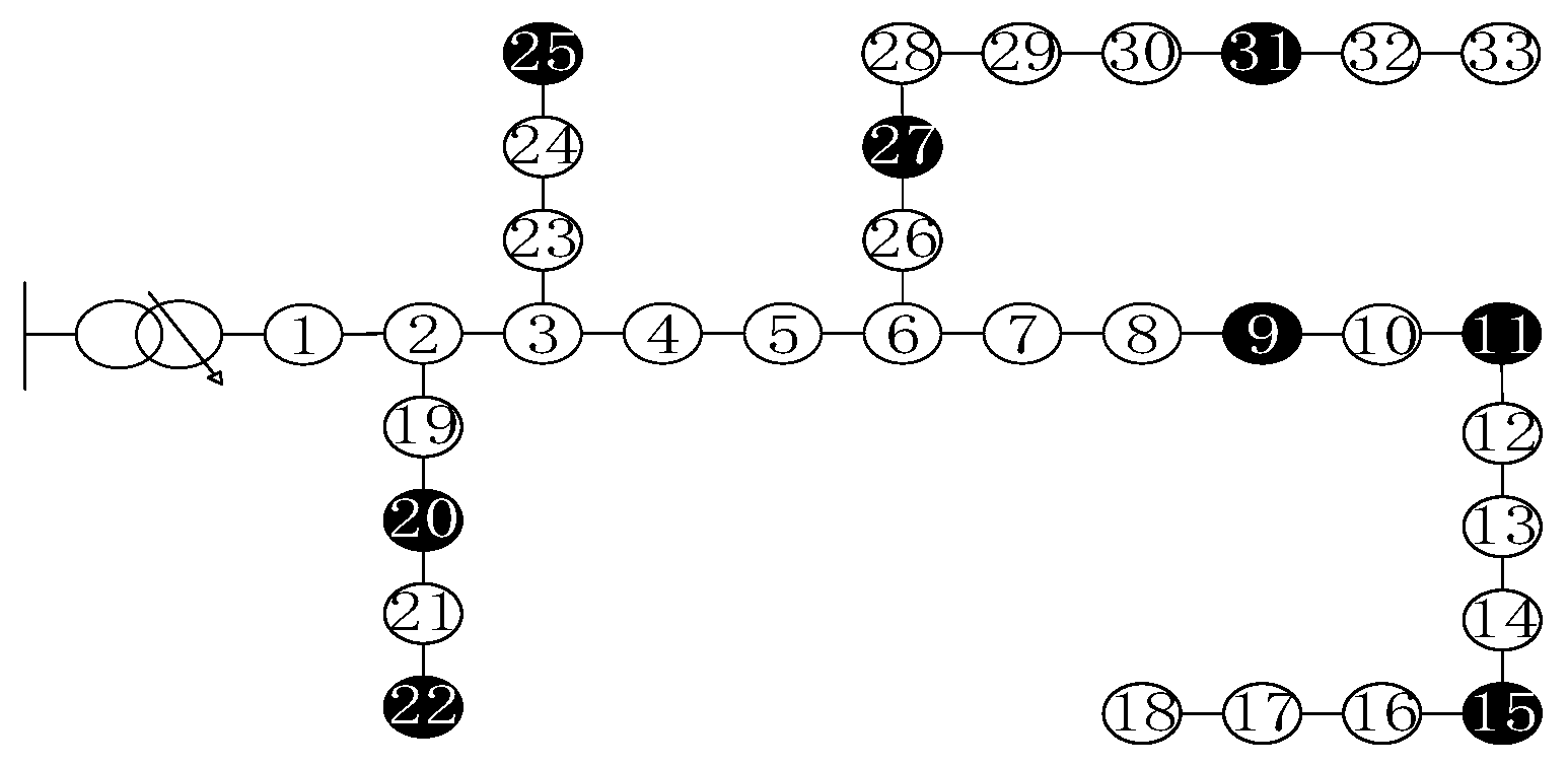
The algorithm proposed in this paper has been validated through comprehensive testing on the IEEE 33-node distribution system. The system’s topology is illustrated in
Figure 6, with white circular markers denoting load-only nodes, and solid black markers indicate nodes equipped with PV systems. Each node is labeled with its corresponding identification number (1–33), and the interconnecting lines represent the distribution feeders forming the radial network configuration.
Each PV-integrated node is furnished with one PV power source. The permissible voltage fluctuation range for all nodes falls within the specified limits [Vi,min,Vi,max] = [0.95,1.05]. Each PV installation at the eight control nodes features identical specifications: The capacity rating is Spv = 1100 kVA, with maximum active power generation capability Ppv = 963 kW under optimal irradiance conditions. Voltage magnitude and line power flow measurements are available at PV-integrated nodes. Additionally, identical measurement functionalities are deployed at nodes 2, 3, and 6, while other nodes in the network lack measurement capabilities.
Voltage control strategy simulations are conducted using four different approaches. These include the proposed adaptive step-based improved dynamic projection dual distributed algorithm, the enhanced dynamic projection dual distributed algorithm, the SFDDFBO algorithm from reference [
22], and a centralized algorithm. Voltage constraints are standardized across all nodes, with upper voltage and lower limits set at 1.05 per unit (p.u.) and 0.95 p.u. The simulation encompasses 80 time steps. To evaluate the efficacy of the proposed strategy in managing voltage profiles and minimizing network losses, two representative scenarios are investigated: scenario 1 representing heavy loading condition and scenario 2 representing light loading condition. These comprehensive test cases demonstrate the robustness of the approach across the range of operational challenges typically encountered in practical distribution networks.
4.2. Scenario 1
In this scenario, under low irradiance conditions, the PV inverter outputs a maximum power of 275 kW. The system operates under light-load conditions at 1.2 times the reference load level. The initial control step size in the proposed Adaptive Step-size Improved Dynamic Projection Primal–Dual Distributed Algorithm (ASIPDDA) is set to 0.25. The Improved Dynamic Projection Primal–Dual Distributed Algorithm and SFDDFBO algorithm share identical parameters with the ASIPDDA.
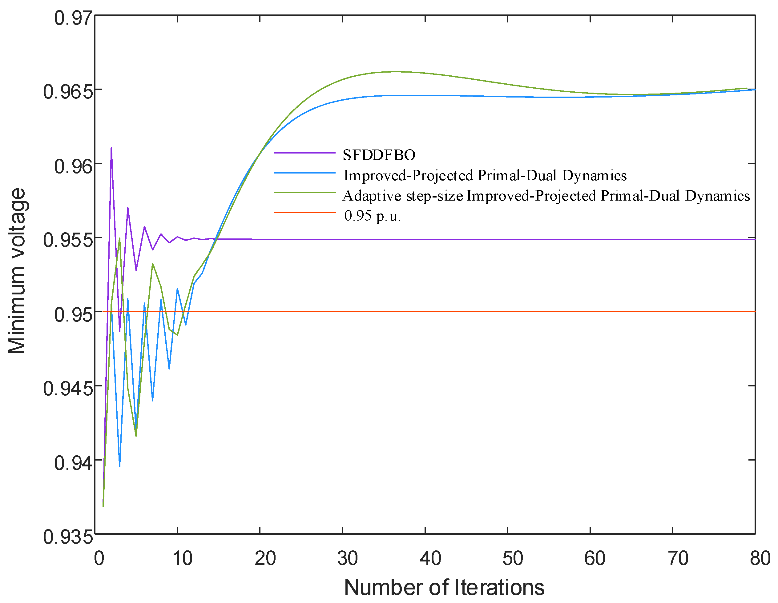
Figure 7 presents the minimum voltage profiles across the network to validate the performance of these three distributed control methods in optimizing network losses. The results demonstrate the efficacy of the proposed approaches.
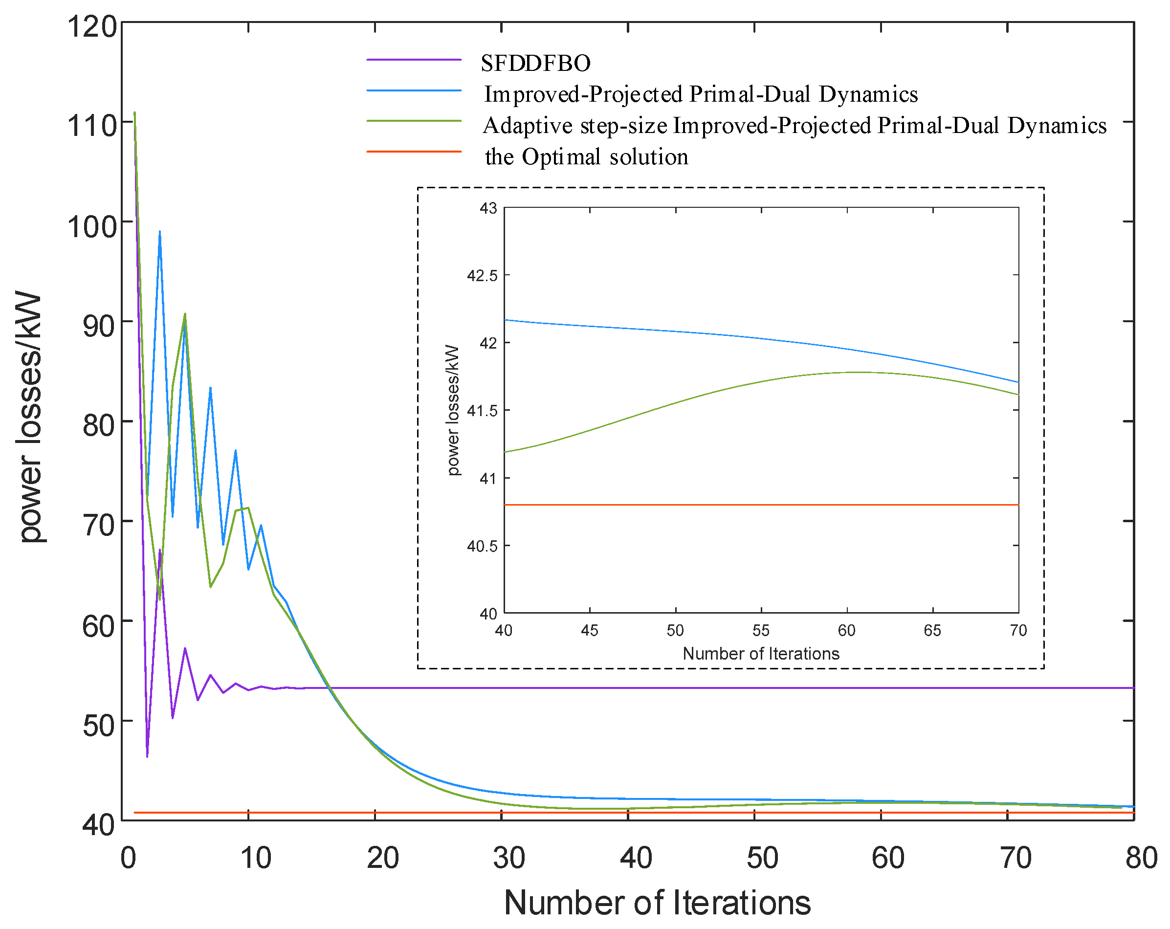
Figure 8 compares the optimization performance of the three distributed control methods against centralized optimization control. It displays the network loss curves obtained from both distributed and centralized control methods under these operating conditions.
Scenario 1 represents heavily loaded network conditions under low PV output. Without PV reactive power regulation, the minimum network voltage drops to 0.937 p.u., accompanied by substantial network losses of 110.7 kW. The control strategy introduced in this paper successfully restores the minimum network voltage within acceptable range after 11 iterations. In contrast, the SFDDFBO algorithm demonstrates faster initial response, achieving voltage regulation within acceptable range after three iterations, while maintaining the maximum voltage levels consistently within acceptable range.
Regarding network loss optimization, the three distributed control algorithms show different performance characteristics. Initially, the control algorithm presented in this paper exhibits lower optimization efficiency compared to the comparative algorithm. However, a significant performance crossover occurs at approximately 15 iterations. After this point, the proposed algorithm demonstrates superior optimization capabilities. It progressively converges toward centralized optimization results. The incorporation of the adaptive step size mechanism notably accelerates algorithm convergence. This represents a significant enhancement to the control structure.
4.3. Scenario 2
A critical test scenario is established to evaluate the algorithm’s performance in mitigating overvoltage risks under light loading conditions. Solar irradiance reaches its maximum level while the load is set at 90% of the reference load. The control parameters for both the algorithm presented in this paper and SFDDFBO are maintained consistent with specifications detailed in
Section 3.2.
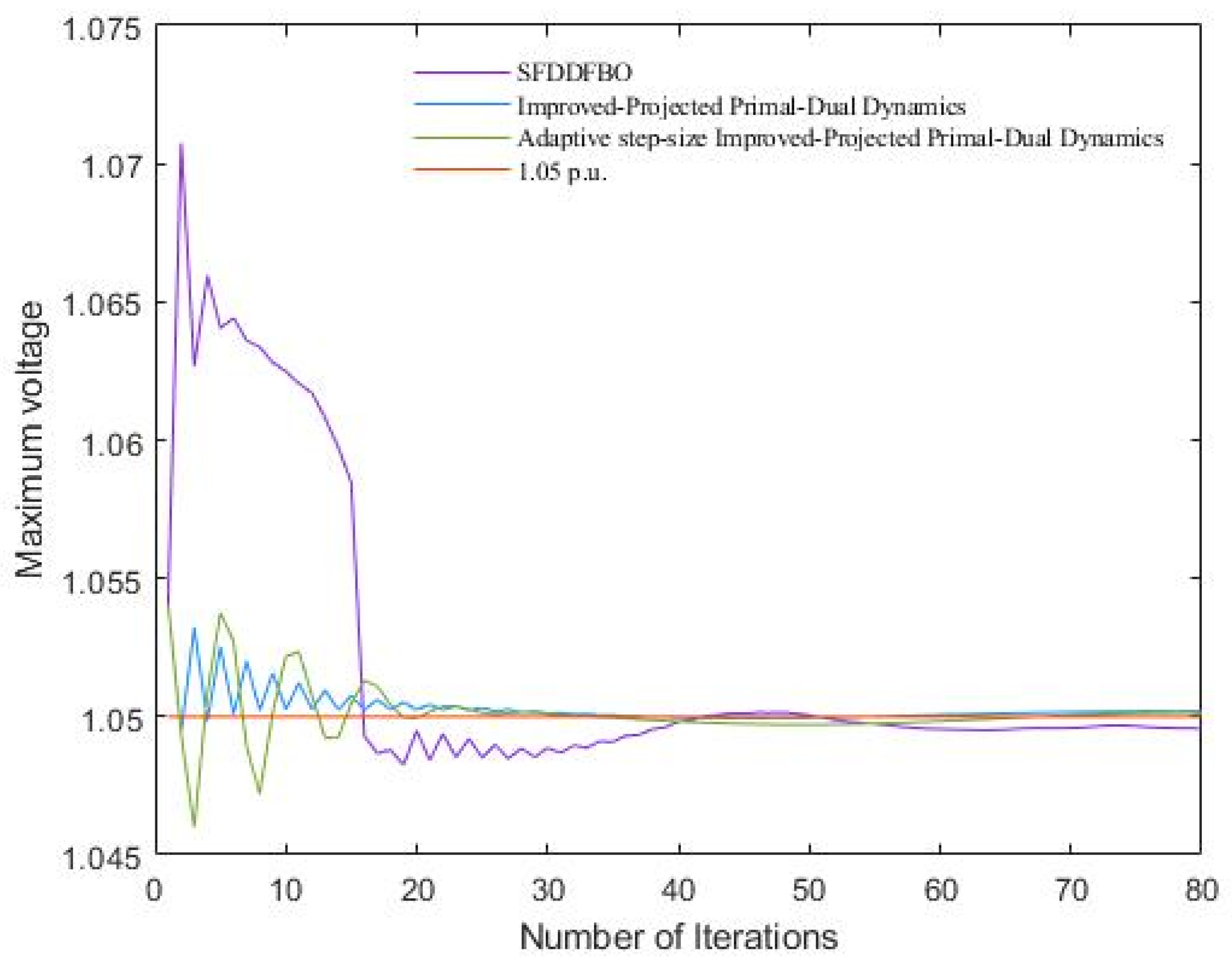
Figure 9 presents the comparative performance evaluation of the three distributed control methodologies in addressing voltage limit violations. It tracks the temporal evolution of maximum network voltage levels achieved by each control method throughout the iterative control process. The results demonstrate the dynamic response characteristics and convergence properties of each approach.
Figure 10 provides a comprehensive assessment of the optimization capabilities. It presents a comparative analysis of network loss profiles generated by the two distributed control methods against the centralized control method.
It is evident that in scenario 2, without photovoltaic reactive power regulation, the maximum network voltage reaches 1.054 p.u. The control strategy introduced in this paper successfully restores the minimum network voltage within acceptable range after 26 iterations. In contrast, the SFDDFBO algorithm demonstrates faster initial response, achieving voltage regulation within an acceptable range after 16 iterations. This comparative analysis validates that the proposed control strategy effectively maintains voltage stability when confronting upper limit violations, provided that sufficient reactive power capacity is available in the system.
Regarding network loss optimization performance, a notable difference exists between the comparative algorithm and the optimal network loss. Specifically, after 80 iterations, the control algorithm presented in this paper yields network losses that are approximately 3 kW higher than those achieved through centralized optimization. This variance can be attributed to the inherent limitations of scenarios with partial measurement coverage, where network losses cannot be directly measured at all nodes. The optimization model employs approximation techniques to compensate for incomplete measurements, which inevitably introduces minor computational errors relative to centralized optimization results. However, these deviations remain well within acceptable engineering tolerance ranges and do not compromise the practical applicability of the proposed method.
In distribution systems, voltage deviations beyond ±5% of nominal values should be corrected within 1–2 min to prevent equipment damage and maintain power quality standards. Given typical control cycle times of 0.5 s, our algorithm’s convergence within 11–26 iterations represents response times of 5.5–13 s, well within acceptable tolerance.
4.4. Twenty-Four-Hour Simulation
A comprehensive validation framework for the algorithm’s performance was implemented utilizing high-resolution temporal data acquired from a representative geographical location. The primary dataset encompasses normalized measurements of photovoltaic generation and load demand, sampled at 15 min intervals over a complete diurnal cycle. Linear interpolation methodology was applied to both the generation and demand profiles, yielding minute-resolution time series data. The validation framework incorporates a system configuration where individual photovoltaic units are characterized by a maximum power generation capacity of
Ppv = 963 kW under peak solar irradiance conditions. The evolution of both photovoltaic power output and system load profiles is visualized in
Figure 11 and
Figure 12, respectively.
For the control algorithm introduced in this study, the initial control step size is set at 0.25, with acceleration factors b = 2 and c = 20 and step-size correction factors α = 1.005 and β = 0.85. We assume that each control operation consumes 0.5 s. Performance analysis is visualized in
Figure 13,
Figure 14 and
Figure 15.
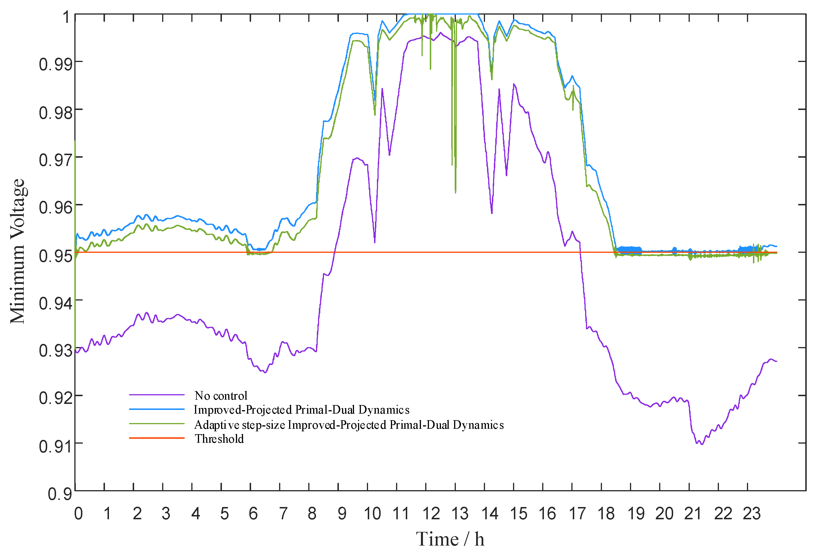
Figure 13 and
Figure 14 present comparative voltage profiles. These figures illustrate the maximum and minimum network voltages achieved under both the proposed control strategy and the baseline case without reactive power control.
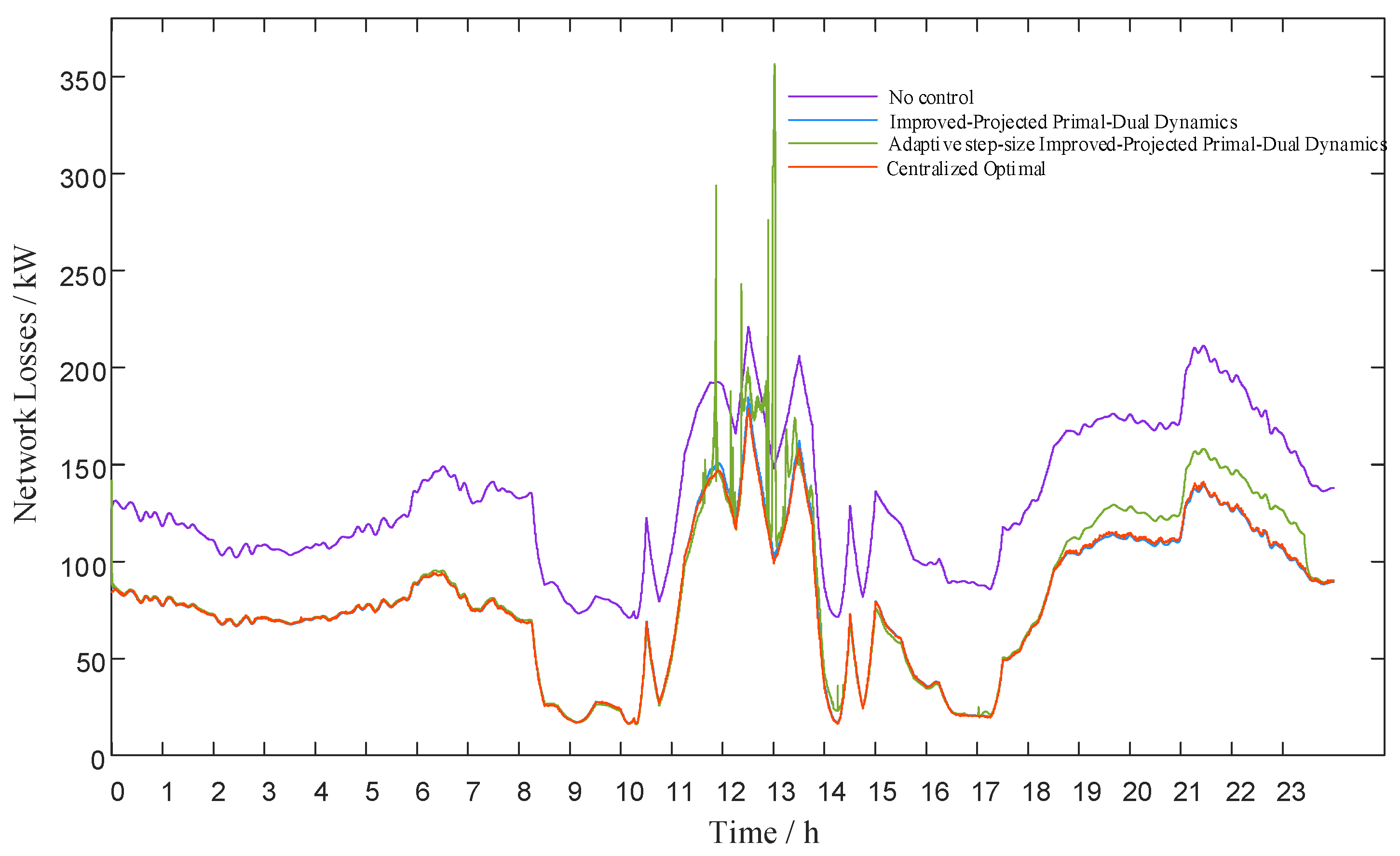
Figure 15 assesses the optimization efficiency of the distributed control method suggested in this paper versus centralized optimization control. It illustrates network loss curves produced by three scenarios: the distributed control method, no reactive power control, and centralized control method.
As depicted in
Figure 13 and
Figure 14, the adaptive reactive power control method proposed in this paper effectively mitigates voltage violations. In contrast, the control algorithm without adaptive step size exhibits minor overvoltage limit violations between 11:00 and 14:00. The maximum overvoltage reaches 1.0504 p.u. During periods of minimal solar irradiance, the system encounters under-voltage conditions. The voltage level drops to 0.9497 p.u. Moreover, the control algorithm of non-adaptive step size displays significant voltage fluctuations during these transitional periods. Therefore, the integration of adaptive step size control efficiently addresses voltage fluctuations issues during the control process.
As illustrated in
Figure 15, the reactive power control method introduced in this study significantly reduces network losses. This reduction is substantial compared to scenarios without reactive power control. When compared to centralized optimization results, the network loss profiles demonstrate remarkable agreement between the two methods. The proposed distributed reactive power control strategy incurs marginally higher losses than the centralized optimization method. However, this difference is negligible. This close alignment in performance validates the effectiveness of the distributed control strategy. It successfully approximates centralized optimization performance while maintaining the advantages of a decentralized architecture.


