Nowcasting Solar Irradiance Components Using a Vision Transformer and Multimodal Data from All-Sky Images and Meteorological Observations

Abstract

As the solar share in energy generation is expanding globally, solar nowcasting is becoming increasingly important for the efficient and economical management of the power grid. This study leveraged the spatial context provided by all-sky images (ASI) in addition to the meteorological records for improved nowcasting of global, direct, and diffuse irradiance components. The proposed methodology consists of two branches for processing the multimodal data of ASIs and meteorological data. Due to its capability of understanding the overall characteristics of the image through self-attention, a vision transformer is utilized for the image branch while normal dense layers process the tabular meteorological data. The proposed architecture is compared against the baselines of the Ineichen clear sky model, a feedforward neural network (FFNN) where cloud coverage is computed from the ASIs by a simple color-channel threshold algorithm, and a hybrid of FFNN and U-Net model, which replaces the color threshold algorithm with fully convolutional layers for cloud segmentation. The models are trained, validated, and tested using the quality-assured ground-truth data collected in Ulaanbaatar, Mongolia, from May to August 2024, under one-minute intervals with a random split of 70%, 15%, and 15%. Our approach exhibits superior performance to baselines with a significantly lower mean absolute error (MAE) of 15–33 W/m² and root mean square error (RMSE) of 26–72 W/m², thus potentially aiding grid operators’ decision-making in real-time.

1. Introduction

1.1. Solar Irradiance Nowcasting

The 21st century is witnessing a significant shift in the energy infrastructure from a fossil fuel-dominant system to a non-fossil fuel-based one focusing more on renewable energy. Compared to 21.7% in 2014, on a global scale, the share of renewable resources for electricity generation increased to 30.3% in 2023, surpassing the increase in power demand [1]. This highlights the rapid development of variable renewable energy (VRE) resources in the last decade, incentivized by the Paris Agreement at the 21st Conference of Parties (COP21) of the United Nations Framework Convention on Climate Change (UNFCCC) in 2015 [2]. Solar energy is of particular interest for climate change mitigation and maintaining the global average temperature within 2 °C above the pre-industrial level. Thanks to technological advancements and supportive policies, solar technologies are becoming more affordable, thereby expanding globally [3]. In the case of Mongolia, as shown in Figure 1, renewable capacity has continuously been added since 2017; before that, it consisted of wind and hydropower only. Furthermore, 2017 marked the commissioning of the first mega-scale photovoltaic (PV) power plant in the country, and since then, yearly PV generation has increased steadily. As of 2023, PV constitutes 25% of renewable generation with 193 GWh, which is almost 10 times higher than 19.7 GWh in 2017 [4]. Therefore, it is anticipated that PV will be one of the major generation sources in the global energy mix for the years to come.

Despite all the appealing sides, the most significant drawback of solar energy is its inherent instability, caused mainly by clouds, which leads to economic loss if not managed carefully. For example, in a power network consisting of a large share of PV, reserves are kept to back up in case of ramp events, or excess PV generation is curtailed when the demand is lower. Fortunately, solar irradiance nowcast can help overcome this shortcoming by supporting decision-making in real-time electricity dispatching [5,6]. Nowcasting, also known as very short-range forecasting, is defined by the World Meteorological Organization (WMO) as the description of the current weather situation up to 6 h ahead in the future time horizon [7]. In the solar energy sector, nowcasting is often focused on future time scales of up to 20 min, which allows grid operators to manage the network of multiple bodies effectively under real-time constraints [5,6].

1.2. Related Works

The current status quo of solar irradiance nowcasting is to utilize the all-sky, also known as the whole sky and total sky imager; thanks to its wide view angle and frequent retrieval (usually every minute), cloud movement in the surrounding area can be monitored and projected into the near future. Owing to the high upfront cost of the specialized all-sky imaging systems for solar applications, several studies have attempted to reduce the cost, such as by assembling components in a do-it-yourself (DIY) method [8] or designing a new catadioptric system by attaching a downward-facing camera above the reflective dome to capture sky images [9]. Particularly, the use of surveillance cameras is reported frequently [6,10,11,12]. In short, all-sky camera-based solar nowcasting in the literature can be divided into three subgroups in terms of the cloud detection methodology: (i) fixed or adaptive thresholds applied to color channels, (ii) clear sky library (CSL) to differentiate the clear and cloudy sky based on the solar position and atmospheric constituents, and (iii) use of machine learning for learning representations from the all-sky images (ASI) effectively.

One of the earlier studies was conducted by Marquez et al., where the authors proposed an intra-hour direct normal irradiance (DNI) forecasting methodology based on total sky images. First, cloud pixels are identified by the adaptive threshold of the color channel ratio of red to blue. Then, grid cloud fractions are computed from the origin of the sun to the reverse wind direction, which are determined by overlapping consecutive images. Finally, DNI is predicted via the multiplication of the clear sky DNI by the computed grid cloud fractions, where each grid represents the future cloud fraction 3–15 min ahead in the future. When evaluated on four selected days from different seasons in California, the proposed methodology outperformed the persistence model, especially in the horizon of 5 min ahead, where the root mean square error (RMSE) was around 300 W/m². Thus, the authors noted the applicability of the total sky imager for short-term forecasting and discussed further research directions such as applying machine learning methodology for correctly classifying cloud pixels, especially near sun glare areas, and considering multi-layer cloud structures by stereo photography with multiple ground-based imagers [13].

Aside from the full electromagnetic spectrum of the solar irradiance, the visible region can also be interesting to investigate since the photosynthetically active radiation (PAR) covering the visible light spectrum plays a crucial role in plant growth, thus it is an important topic for the agricultural sector. In addition, the light use efficiency is high under cloud presence, making the diffuse component valuable. In a study by Yamashita et al., the authors derived cloud cover, sun appearance, and sky brightness from the ground-based whole sky images, which are then used to estimate the global and diffuse photon flux density from the simultaneous solar irradiance measurements [14].

By virtue of advancements in artificial intelligence (AI), there are a growing number of studies that process ASIs by machine learning algorithms and neural networks. Scolari et al. implemented principal component analysis (PCA) to derive the most important features from the ASIs for the estimation of the global horizontal irradiance (GHI). They found that 26 features, such as average intensity, different color channel representations, and their ratio, represent 99.5% of the total variance in the sky image collected for 20 days. The derived principal components are further processed by a simple neural network of a single layer with 10 neurons to output the clear sky index, which is multiplied by the clear sky irradiance for the GHI estimation. As a result of evaluating the cross-validated model for 15 days in all seasons of 2017 under time granularities of 1, 5, and 15 min, it was found that the model receiving features derived from ASIs as input resulted in the best performance. Even adding satellite-derived features did not improve error metrics, and the ASI-based model was better than the well-established Heliosat-2 estimation by 20–45%. This shows the superiority of the ASI-based model owing to its higher spatial and temporal resolution [15].

One of the most used deep learning architectures for image processing is the convolutional neural network (CNN). Thus, it is also investigated for analyzing ASIs, especially for cloud segmentation, since it is the fundamental step before proceeding to nowcasting. Xie et al. proposed a cloud segmentation model named SegCloud composed of fully convolutional layers [16]. Its architecture is similar fashion as with the U-Net model first developed for medical image segmentation [17]. The U-shaped convolutional layers consist of an encoder and decoder part that extract high-level abstract features from images and then translate them back to the original dimension. For the cloud segmentation task, this model performed superior to conventional methods such as color channel ratio and adaptive threshold. This agrees with the findings of Hasenbalg et al., who benchmarked six cloud segmentation algorithms and found that the fully convolutional network based on the VGG-16 architecture resulted in the best performance with 97% accuracy on 160 test images of different sky conditions. However, ASIs are cropped to a rectangular shape in order to fit into the model, which loses information about the outer sky horizon [10].

Fabel et al. approached the cloud segmentation task with a slightly different technique known as self-supervised learning. Instead of relying on a small amount of labeled data to model the relationship between the input features and target output, the self-supervised learning method provides a large amount of unlabeled data from which the model is supposed to learn useful representations that would later be transferred to downstream tasks. The authors designed pretext tasks for representation learning from unlabeled ASIs, such as the deep cluster method for iteratively clustering outputs provided by the convolutional network with ResNet34 encoder, where skip connections help train deep CNN effectively [18]. Additionally, in painting, and super-resolution method fills the gap in the image while the super-resolution approach recovers the original pixel resolution from the intentionally blurred one, which helps in learning the overall context of the images. The learned representations are then fine-tuned by the U-Net model [17] and 770 labeled ASIs for semantic cloud segmentation, which not only detects clouds but also classifies them into three groups based on their heights. The authors noted the promising result of pixel accuracy of 85.8% on average and surpassing the CSL method by 7% for binary segmentation [12].

Despite the growing interest in using AI for cloud detection, there exist non-machine learning methods such as simple color channel-based algorithms [19] and more intricate CSL [10,20,21,22]. For example, the red–blue ratio (RBR) method classifies pixels into clouds if the ratio of the red to blue color intensity is higher than a certain threshold, which is dependent on the camera system and the location. The reasoning behind this is that the clear sky mostly appears blue due to dominant Rayleigh scattering, while under clouds, the blue channel becomes less prominent because of Mie scattering. Despite its simplicity, the RBR method works well when there is a clear distinction between the sky and clouds, but it suffers in high zenith angles due to increased brightness of the sun region and with thin or high altitude clouds whose RBR characteristic is similar to that of the sky. The working principle of the CSL is also simple, by differentiating the current sky image from what would appear under the clear sky with the same solar position and atmospheric loads. However, there is no global CSL because it is dependent on local atmospheric conditions. Therefore, when applied to a different region than the origin site, it needs to be adjusted or newly built by the local ASIs and atmospheric properties.

Some researchers developed a hybrid model to further improve the solar irradiance nowcasting accuracy. For instance, Nouri et al. proposed a hybrid model of ASI-based nowcast and the persistence model for a lead time of up to 20 min ahead. The ASI-based branch is a stereoscopic approach, making use of two sky cameras for cloud geolocation, which provides cloud height information. The clouds are detected by the CNN and then tracked by correlating consecutive images. At last, the cloud shadow is projected onto the lead time, resulting in the GHI estimation map covering a 60 km² area. On the other hand, the persistence branch assumes the change of only solar position, that other factors remain the same for lead times. The final GHI nowcasted map is the combination of the two nowcasts by the accuracy weighting. The authors evaluated the model’s performance for eight different sites located in the region of interest and for all lead times. It was found that the hybrid model outperformed the single persistence or ASI-based model, even when spatially aggregated. Therefore, adding more sky cameras to establish a dense ground network is discussed for detecting clouds in different layers, which would potentially improve the current nowcast approach and increase the lead times [11]. Furthermore, one of the most common combinations is CNN and long short-term memory (LSTM). Hou et al. and Lim et al. investigated the use of CNN-LSTM for solar irradiance or power prediction, where the CNN model is used to classify the weather condition, while the LSTM model is used to predict the future values [23,24].

Although the downward shortwave radiation affects the PV output the most, the most important info for grid operators is the PV generation amount. On that account, some experiments are conducted to directly estimate the PV power output from ASI data by exploiting the convolutional layers for feature extraction, which are then processed by the fully connected dense layers to make the final prediction. The model architecture is fine-tuned to find the optimal number of convolutional and dense layers, and the input image resolution, etc. The resulting test relative RMSE was 26–30.2% for PV power estimation, while the forecast skill for 15 min ahead forecasting was 15.7%, indicating improved performance than the persistence model [25,26,27].

1.3. The Contributions of This Study

The breakthrough of the attention-based transformer has revolutionized neural network architectures. By enabling learning of the long-range dependency in the input sequence through the self-attention mechanism, it overcomes the limitations of the previous state-of-the-art architecture, LSTM, whose gating mechanism restricts attending distant tokens [28]. Dosovitskiy et al. proposed a version of the transformer model for image processing, known as the vision transformer (ViT), which outperformed the previous state-of-the-art CNN models with less computation [29]. However, the examination of the transformer architectures for ASIs representing local sky conditions is still limited. Recent studies by Liu et al. and Mercier et al. investigated the transformer-based approach for short-term GHI forecasting up to 30 min ahead provided by the preceding ASIs. In spite of that, the less frequent retrieval of ASIs every 5 or 10 min might not be adequate for modeling the fast-fluctuating solar irradiance [30,31].

This paper aims to address this research gap by focusing on the vision transformer method for ASI-based solar irradiance nowcasting under a time granularity of one minute. It is expected to result in improved performance with the help of transformer architecture, which focuses on different aspects of the images simultaneously through multi-head self-attention. Therefore, this study contributes to the solar irradiance nowcasting field by (i) implementing the vision transformer architecture to derive highly informative features from the ASIs in addition to the meteorological records, (ii) benchmarking the proposed framework against the commonly used clear sky irradiance and deep learning models, and (iii) predicting not only the global irradiance but also the direct and diffuse components which are highly relatable for concentrating solar power and agricultural sectors, respectively, but less explored in the literature.

Due to the temporal discontinuity of the collected data, here we estimate solar irradiance components from the corresponding multimodal data, meaning the lead time is none. However, it should be noted that the proposed multimodal learning has the potential for extension to predict solar irradiance and solar generation amount in the short-term horizon by adding a temporal dependency. This paper is organized as follows: the multimodal data and the preprocessing routines are presented in the next section, the proposed solar irradiance nowcasting model is described in Section 3 along with baselines, Section 4 evaluates the modelling techniques using standard error metrics and investigates the proposed methodology in more detail, and finally conclusions are discussed in Section 5.

2. Dataset

2.1. Multimodal Data

The multimodal data, consisting of ASIs and meteorological measurements, are provided by the observatory located on the rooftop of the National University of Mongolia, Ulaanbaatar (47.92° N, 106.92° E), as shown in Figure 2. The data collection duration is from 24 May to 12 August 2024, and the time step is one minute.

2.1.1. Meteorological Measurements

On the one hand, meteorological measurements consist of wind speed and direction, ambient temperature, relative humidity, vapor pressure, dew point temperature, and solar components (global, direct, and diffuse). The upper part of Figure 2a shows the weather station that records all meteorological parameters except the DNI and diffuse horizontal irradiance (DHI), which were measured by the pyrheliometer and shaded pyranometer, as shown in Figure 2b. While the global irradiance was measured by the Hukseflux CHF-SR11 class B pyranometer [32], the direct and diffuse components were monitored by the class A actinometers of EKO Instruments, namely MS-57 pyrheliometer and MS-802F pyranometer with a shading ball attached to the STR-22G solar tracker [33]. We quality controlled the solar irradiance measurements following the comparison test of the Baseline Surface Radiation Network (BSRN) [34], which is based on the ideology that the global irradiance equals diffuse plus zenith corrected beam component. Physical limits were also taken into account, such that solar irradiance components cannot have negative values, and when the solar zenith angle (ZA) is more than 93 degrees, the nighttime irradiance should not exceed 20 W/m². As shown in Equation (1), the quality check thresholds are more relaxed, with added tolerance considering sensor calibration errors and thermal offsets such that allowing the GHI to be lower than DHI up to 150 W/m² and higher than DNI + DHI by up to 15% or 150 W/m² due to cloud enhancement effects. Lastly, the closure test checks the physical consistency within the solar irradiance components by permitting up to 8% uncertainty in the measured GHI, and not fulfilling it indicates an erroneous measurement in one or more components. As a result, 77,496 samples were validated out of 87,017 measurement records.

$$\left\{\begin{array}{c}\begin{array}{c}\mathrm{GHI}\ge 0,\mathrm{DNI}\ge 0,\mathrm{DHI}\ge 0\\ \mathrm{If}\mathrm{ZA}°>93;\mathrm{GHI}\le 20,\mathrm{DHI}\le 20,\mathrm{DNI}\le 20\\ \mathrm{GHI}+10\ge \mathrm{DHI}\end{array}\\ \mathrm{GHI}\le \mathrm{DNI}+\mathrm{DHI}+\max \left(\right(\mathrm{DNI}+\mathrm{DHI})\times 0.15,150)\\ \mid \mathrm{GHI}-(\mathrm{DHI}+\mathrm{DNI}\times \cos (\mathrm{ZA}\left)\right)\mid \le 0.08\times \mathrm{GHI}\end{array}\right.$$

(1)

Figure 3 shows the validated readings of solar irradiance components after discarding suspicious measurements. That way, uncertainties of the target variables are minimized, which is crucial for the development of the nowcasting model, as well as evaluation. It is noticeable that the DNI readings become close to 0 W/m² on overcast days when the direct irradiance is blocked by very thick clouds; thus, diffuse-dominated irradiance reaches the ground surface, which fulfills the criteria of GHI should be greater than or equal to DHI with some margin.

Figure 4 shows the distribution of meteorological parameters that are regarded as explanatory variables for the solar irradiance nowcasting. Furthermore, Figure 5 shows the correlation matrix between these input features and target outputs. Whilst the ambient temperature positively correlates with all solar irradiance components, the relative humidity shows a negative correlation. Although the correlation degrees are modest, the GHI component shows a slightly stronger correlation than the DNI and DHI.

2.1.2. ASIs

On the other hand, there are sky images recorded by the Mobotix Q26 hemispheric camera equipped with a fisheye lens of 180° view angle, as shown in the foreground of Figure 2a [35]. The images are provided by the 6MP CMOS sensor in the RGB color space with a resolution of 3072 × 2048. The sky camera is set to not record the images from 21:00 to 3:59 to exclude nighttime. In addition, unfortunately, a two-hour-long measurement from 15:00 to 15: 59 and 17:00 to 17:59 is not recorded due to a setting misconception. Nevertheless, after discarding any missing timestamps, the multimodal data is preprocessed for nowcasting solar irradiance components.

2.2. Data Preprocessing

Since date time, solar position, and clear sky irradiance values are relevant for the current exercise, we derived the hour of the day, minute of the hour, day number, solar zenith and azimuth angles, and clear sky irradiance for global, direct, and diffuse irradiance components, as additional input features. For that purpose, the Python pvlib 0.10.4 library’s default Ineichen clear sky model with climatological turbidity was used [36]. Moreover, Figure 6 shows the sample ASI and preprocessing steps. It is a common practice to remove non-sky objects such as nearby buildings and trees by masking [13,15]. Also, images were cropped to retain the bounding box of the sky horizon only, and then resized to 512 × 512 to speed up further processing. Moreover, it is evident that obtaining useful information from the sun glare area is difficult due to the saturated pixel brightness surrounding the sun. Nonetheless, this study aims to acquire a feature representative of the present atmospheric condition from the ASIs.

Before training a neural network model, input features and output targets are normalized, which helps with efficient weight updates by the backpropagation algorithm as the learning progresses. Then, data samples are randomly shuffled for a more robust evaluation of the proposed model. This guarantees that the model will be exposed to different dates and times and sky conditions in the training and evaluation phases. A total of 77,496 meteorological and ASI data pairs were randomly split into the training, validation, and testing sets with a ratio of 70%, 15%, and 15%, respectively. This ensures that sufficient data was provided for learning the local solar climate and testing the model’s capability on never-seen data. The validation data serve multiple roles, such as hyperparameter tuning, model selection, and checking generalization capability, which is important to prevent overfitting.

3. Methodology

3.1. Baselines

For benchmarking, the Ineichen clear sky model, a simple feedforward neural network (FFNN), and a hybrid of U-Net and FFNN were selected as baselines.

3.1.1. Clear Sky Model

As mentioned in Section 2.2, the Ineichen clear sky model assumes climatological turbidity by default and only requires date, time (including time zone), and location (latitude, longitude, and altitude) as inputs [36]. Due to its simplicity, the clear sky model was considered one of the baselines.

3.1.2. FFNN

The FFNN model receives the cloud cover as a supplementary feature derived from the ASIs in addition to the meteorological and solar-positional parameters. The cloud cover is the ratio of the number of cloud pixels to the number of total pixels in the sky horizon. The cloud pixels are detected via the simple color channel-based method of RBR [19]. A threshold of 0.9 is set based on visual inspection for separating sky and cloud pixels. Consequently, the FFNN processes the 15 input features through a series of non-linear transformations defined in hidden layers to predict the solar irradiance components.

The loss function is the mean square error (MSE). Harnessing the validation set, the optimal hyperparameters are found by the grid search method, which tests different combinations of hyperparameters such as the number of neurons in the dense layers. As a result of the fine-tuning, the final model architecture is obtained that produces the lowest MSE in the validation split. As illustrated in Figure 7, the resulting FFNN consists of 2 hidden layers, each with 128 and 64 neurons, activated by the rectified linear unit (ReLU) activation function to introduce nonlinearity. The bottleneck structure forces dimension reduction by keeping the most essential information for further processing and discarding redundant features, which lowers computational complexity as well.

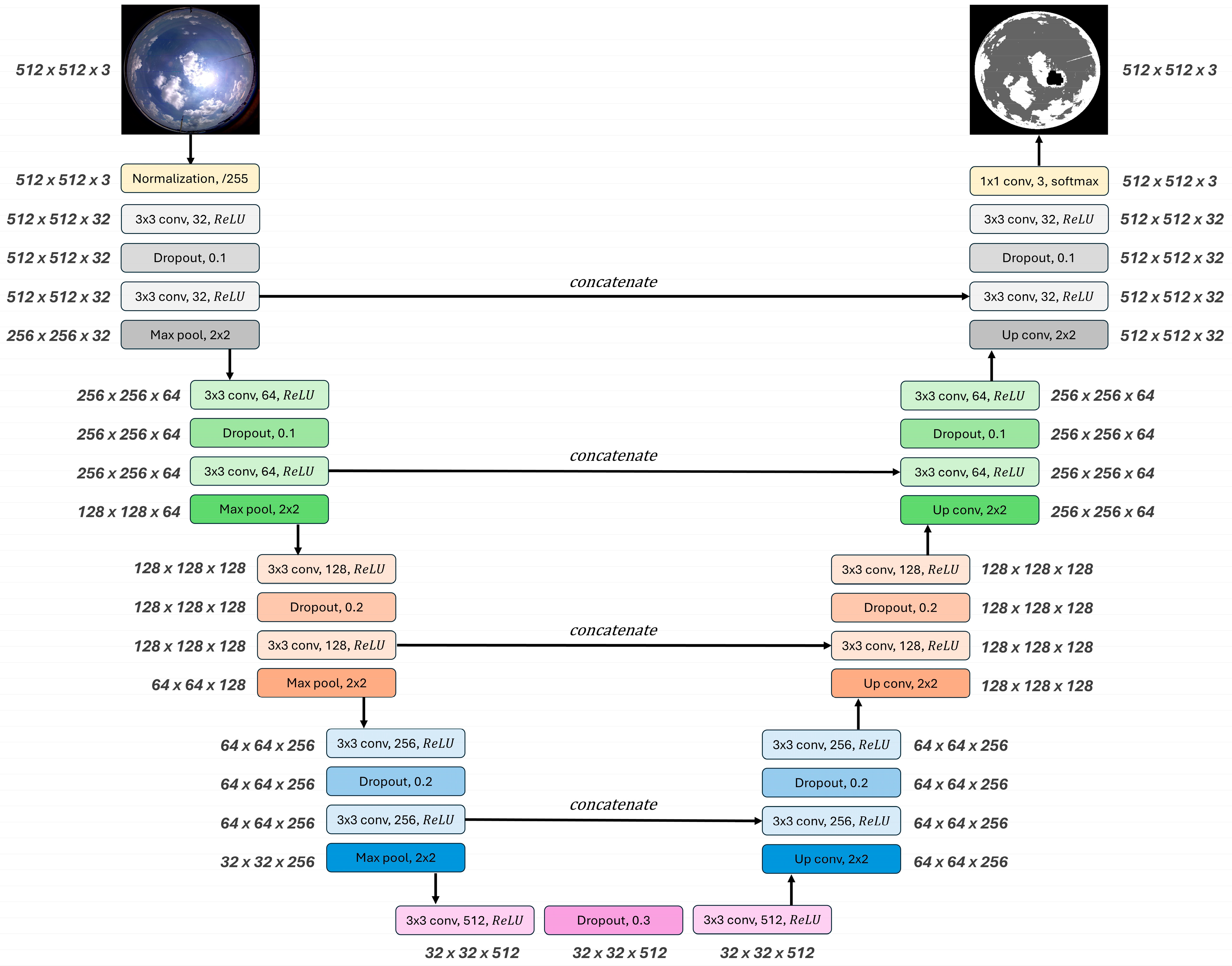
3.1.3. Hybrid of FFNN and U-Net

The hybrid model’s structure is the same as with FFNN, except that the cloud cover is computed with the help of the U-Net model [17]. It is hypothesized that extracting high-level abstract features through a series of convolutional layers of U-Net will result in improved cloud segmentation compared to the simple RBR method, which suffers from false detection of clouds in the sun glare region and misclassification of high-altitude cirrus clouds as sky due to their similar RBR characteristics. Since our data do not include annotated ASIs, the Whole-Sky Image SEGmentation (WSISEG) database, consisting of 400 ASIs and their corresponding masks, was used for training the U-Net model. There are 3 classes of sky, cloud, and other objects such as the sun [16]. The original resolution of 480 × 450 was resized to 512 × 512 to match that of ASIs collected in this study. Moreover, 60 images of 10 clear skies, 10 overcasts, and 40 cloudy conditions were saved for independent testing purposes. The remaining images were passed through 5-fold cross-validation to make use of the small number of images. This means that all training data were used for both training and validation, in a way that the data was separated into 5 folds, where one fold was kept for validation and the remaining folds were used for training, and this cycle was repeated 5 times using different folds for validation. Thus, a separate validation set was not necessary to check the generalization capability.

The loss function is the categorical cross-entropy since it is a classification task. Moreover, for model selection, the intersection over union (IoU), also known as the Jaccard index, was used as a selection criterion. It is a statistic ranging from 0 to 1 expressing the similarity between samples. In our case, 0 means there is no overlapping between the predicted cloud segmentation and manually annotated cloud masks, while 1 means precise segmentation.

As shown in Figure 8, the original version was modified by changing input image sizes to 512 × 512, reducing the number of filters in the convolutional blocks, adding dropout layers as a regularization mechanism, and using the same padding to retain the image dimension during the convolution operation for simplicity. On the left side, the contracting path consists of convolutional blocks of 3 × 3 filter size activated by ReLU with an increasing number of filters to capture higher-level features. The max pooling layers downsample the size of feature maps by half. On the right side, the expanding path operates in a reverse direction by upsampling spatial dimensions while halving the number of feature maps. In addition, through the skip connection, it attends to the corresponding blocks in the contraction path to preserve information from both paths, which are further processed by convolutional layers. At the end of the expanding path, 1 × 1 convolution with softmax activation will classify each pixel in the original image into their predicted class using the learned representations, resulting in a segmented image. Finally, same as with cloud detection by the RBR method, the cloud coverage is computed from the segmented image, which is then sent as an input feature to the FFNN described above for estimating the solar irradiance components.

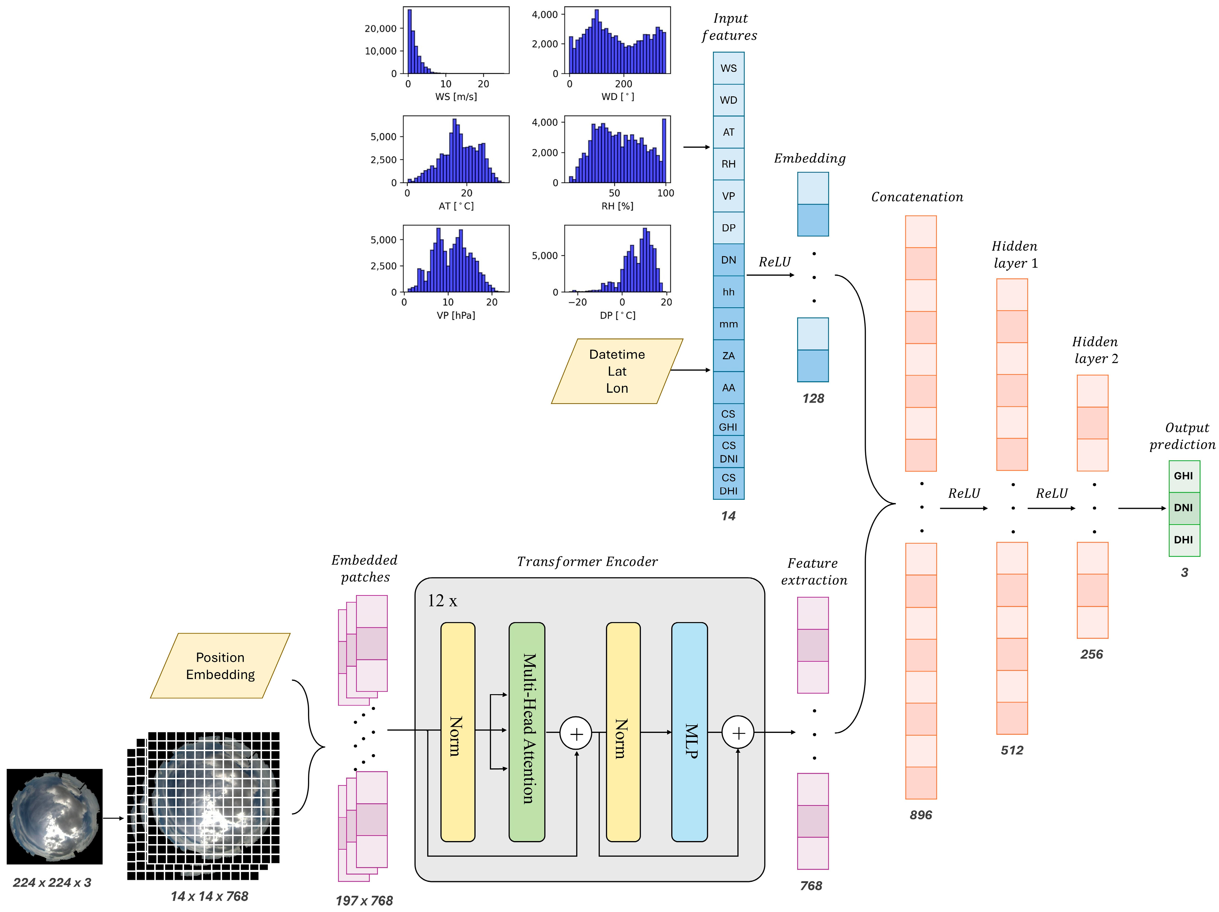
3.2. Proposed Methodology

The proposed framework differs from the baselines by deriving vital features from the ASIs directly with the help of vision transformers, instead of computing cloud cover through cloud segmentation models, thus eliminating the inherent uncertainty resulting from the separate cloud cover estimation. As shown in Figure 9, the proposed methodology processes the multimodal data all together in one model where the vision transformer operates on the image branch, while the tabular data of the meteorological branch is handled by the normal dense layer. The output of both branches is concatenated and processed by the feedforward network to predict the instantaneous GHI, DNI, and DHI.

This study utilized the original vision transformer developed by Dosovitskiy et al. to classify 1.3 million images of the ImageNet dataset into their corresponding classes of 1000 categories [29]. It is based on the reasoning that the images can be seen as sequences of image patches; thus, the attention mechanism can be applied to learn their interdependencies, to finally grasp the whole picture. The ViT Base 16 architecture with pre-trained weights was implemented due to its light weight compared to other versions. In a complicated classification task of 1000 classes, it resulted in 81.07% top-1 accuracy, meaning the correct label matches the model’s prediction when only the highest probability is taken into account. This increased to 95.32% top-5 accuracy, which means the true label is found within the top-5 probability scores out of all 1000 scores for each category [37]. Therefore, although our goal is not to classify sky images, we presuppose that the strong general features obtained through transfer learning would aid in predicting solar irradiance components by providing the image summary. Following the original settings, the ASIs are resized to 224 × 224, which would be further divided into 14 × 14 image patches of 16 × 16 resolution. Then, it is flattened with a positional embedding to be processed by the transformer encoder, which outputs hidden dimensions of 768. There are 12 transformer encoder blocks with different focus perspectives, where each consists of multi-head attention followed by an MLP (multilayer perceptron). Same as with the FFNN, the loss function is defined as the MSE, which is the sum of the MSE for all irradiance components.

3.3. Implementation

The NVIDIA RTX A4000 16 GB GPU and Pytorch 2.6.0+cu124 library were used to implement the models described in Section 3.1 and Section 3.2. For the FFNN and U-Net, an adam optimizer with a learning rate of 1 × 10⁻³ was used. The learning rate scheduler was adopted to halve the learning rate when the validation loss plateaus for 10 epochs, and the minimum allowed learning rate was 1 × 10⁻⁵. Additionally, the early stopping callback with a patience of 15 epochs was utilized under 100 epochs to prevent overfitting, meaning that the model will halt the training when the validation loss does not improve for 15 consecutive epochs and recover the best weights found under the minimum validation loss. The optimal batch size was 64 for FFNN and 8 for U-Net, constrained by the GPU memory. For the proposed methodology, an adamW optimizer with a weight decay of 1 × 10⁻¹ was used for gradient update. The learning rate was warmed up for 100 steps, after which the maximum learning rate was 1 × 10⁻⁴ while the minimum learning rate was 0.01 of the maximum. The optimal batch size was 32, and the model was trained for 8 epochs. The fewer training epochs are to reduce the unnecessary computational expense due to the fact that the vision transformer backbone is pre-trained on a large dataset; thus, it needs fewer epochs to converge in a downstream task, unlike training from scratch as in FFNN and U-Net.

4. Results

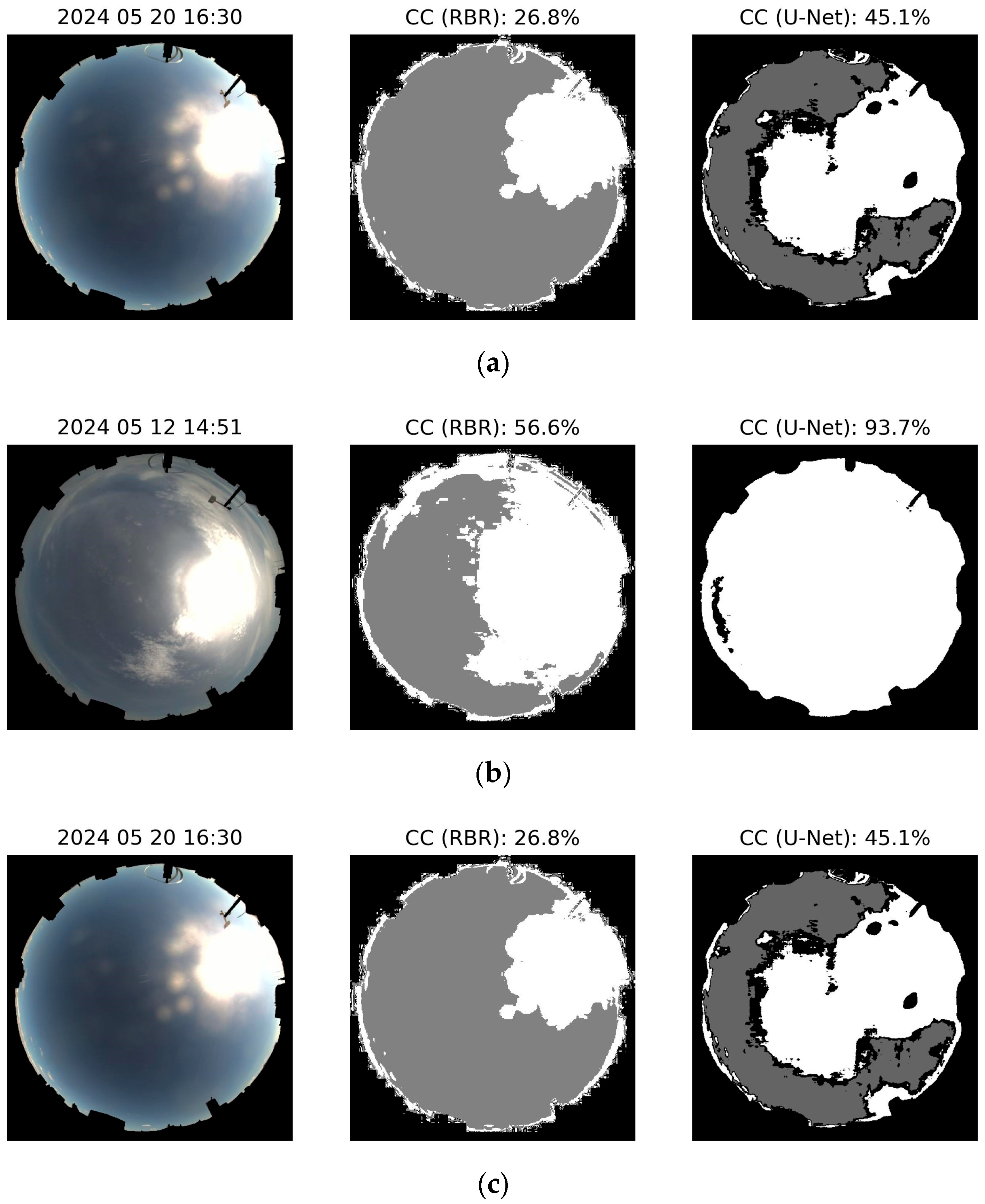
4.1. Cloud Detection

The fine-tuned U-Net model architecture shown in Figure 8 is retrained by utilizing all training images and evaluated independently on 60 test ASIs covering diverse sky conditions. As a result, the test IoU of 0.94 is reported. Although there is a discrepancy in the camera settings and atmospheric background between the WSISEG data and our ASI collection, we presume that the U-Net model would improve the cloud segmentation performance compared to the simple RBR method because of the high-level features learned during the training process. Unfortunately, due to the lack of local cloud coverage recordings, we cannot compare the cloud segmentation results directly. Nonetheless, Figure 10 demonstrates sample ASIs under different sky conditions and the computed cloud coverage by the RBR and U-Net models. It is noticeable that both models suffer from false positive detection of clouds under a clear sky, where the high brightness around the solar disk makes cloud detection challenging. The U-Net model provided additional segmentation of the sun and other non-sky, non-cloud objects painted in black. However, it is misleading to show the sun position because of the different image characteristics of the WSISEG database and our collection of ASIs. The cloud presence multiplied by the high aerosol load makes the clear sky appear less bluish and more grayish, further increasing the difficulty. That explains the significant overestimation of the cloud cover by the U-Net model because it is not exposed to complex ASIs, such as under the influence of heavy haze or fog during the training, as the WSISEG database intentionally excluded them [16]. Under an overcast sky, both models estimate a similar degree of cloud cover. Anyhow, since Figure 10 shows just three examples of cloud segmentations, an extended but indirect comparison is outlined in

Table 1. Benchmarking of solar irradiance nowcasting models on test data at a one-minute time granularity. Error metrics of mean absolute error (MAE) and root mean square error (RMSE) are shown in W/m². Note: N/A stands for not applicable, and the lowest errors are shown in bold.

Models	Parameters	GHI MAE	GHI RMSE	DNI MAE	DNI RMSE	DHI MAE	DHI RMSE
Clear sky model	N/A	129.19	238.20	340.84	475.14	86.65	150.64
FFNN	11,011	49.41	87.50	65.94	115.30	30.04	48.84
U-Net + FFNN	7,760,163 + 11,011	58.75	97.25	80.24	126.93	34.45	55.13
Proposed model	86,392,195	24.90	51.64	32.86	71.67	14.96	25.98
Meteorological data only	200,323	86.17	137.21	163.15	221.72	51.20	78.50
Sky image only	86,324,483	28.26	54.72	32.92	72.43	17.56	29.93

, Section 4.2 by means of assessing the effect of cloud cover computed through the RBR and U-Net models via the estimated solar irradiance components.

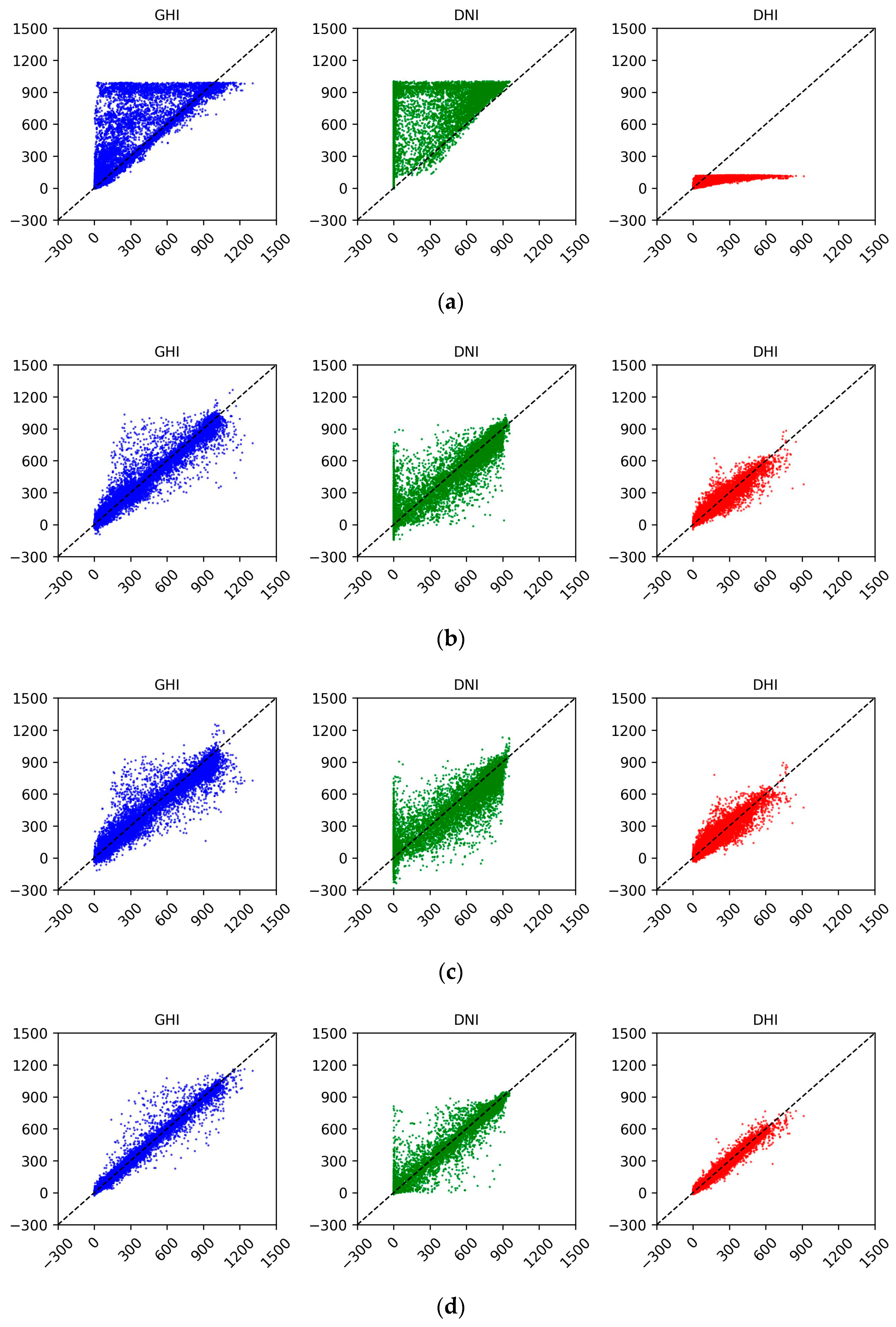
4.2. Performance Evaluation

The mean absolute error (MAE) and RMSE shown in Equations (2) and (3) are selected as evaluation matrices. While measured and predicted irradiance components are denoted as $I_{mea}$ and $I_{pre}$ respectively, $N$ marks the number of pairs between them.

$$\mathrm{M}\mathrm{A}\mathrm{E}={\displaystyle \frac{1}{N}}\sum _{i=1}^N\left|I_{pre}-I_{mea}\right|$$

(2)

$$\mathrm{R}\mathrm{M}\mathrm{S}\mathrm{E}=\sqrt{{\displaystyle \frac{1}{N}}\sum _{i=1}^N{(I_{pre}-I_{mea})}^2}$$

(3)

Table 1 lists the performance comparison of different nowcasting models for each of the solar irradiance components in the test set. The highest errors are found in clear sky models since it does not consider cloud effects, but clouds affect the solar irradiance the most. This is also evident in Figure 11, where the clear sky model overestimates the global and diffuse components while underestimating the diffuse component.

Interestingly, FFNN-based models predict negative solar irradiance values, especially the direct component, caused by the limited capacity of the simple FFNN. This, however, can be addressed easily by adding the ReLU activation function at the final dense layer. Moreover, the FFNN model receiving cloud cover calculated by the simple RBR method performed better than the hybrid of U-Net and FFNN, where the U-Net model segments clouds from ASIs through a series of convolutional layers. We deduce it is not because of the added complexity of the U-Net model but because it is trained and validated on ASIs of different settings and a different background sky than the test ASIs. Therefore, it highlights the importance of exposing similar training and validation data to that of the test set. Otherwise, under just a few training images, the model will struggle to generalize to new test data. Consequently, it would be interesting to train and validate the U-Net model under similar settings of the test data to explore its full potential.

The proposed methodology surpassed all baseline models with significant improvement. In terms of MAE, it resulted in 24–104 W/m², 33–308 W/m², and 15–71 W/m² lower MAE than the baselines for GHI, DNI, and DHI, respectively. The improvement further increased to 35–186 W/m², 41–401 W/m², and 21–123 W/m² for RMSE. Although the training takes longer for the proposed methodology due to the large number of parameters, once online, the inference time is competitive with others. Regarding the solar irradiance components, all models show higher errors for the beam component due to its overall higher values. The opposite trend is observed for the diffuse component, which can also be observed in Figure 11. Moreover, except for the clear sky model, there is a strong under- and overestimation for the direct component, which is partially alleviated by the proposed methodology. The superior performance of the proposed methodology is due to the attention mechanism, as shown in Figure 12, which focuses more on the solar position as it is a primary factor affecting the surface insolation.

4.3. “Hard” vs. “Easy” Scenarios

We further explored when the proposed model performs optimally and sub-optimally. Figure 13 shows the 14 cases when the total error of all irradiance components exceeded 1000 W/m², mostly overestimating the global and direct components when the sun is high in the sky around noon, in black triangles. Moreover, it coincides with a partly cloudy sky condition, especially with clouds near the sun disk. On the other hand, almost perfect estimations are usually found early in the morning or late afternoon, around sunrise and sunset, because of the lower irradiance values at these times. Figure 14 illustrates the highest and lowest error cases from the test set. From the visualized attention, we can see that when the sun is present, the attention is on the solar position and the clouds. Contrarily, when the sun is absent, the attention is on the edge of the sky horizon due to night luminescence by the buildings, etc. Nonetheless, although the attention mechanism on sky images improves predictability, the difficulty of solar irradiance prediction under the cloudy sky condition still remains.

4.4. Ablation Study

An ablation study is conducted to observe the effect of multimodal data on predictive performance. We removed either the meteorological or ASI branch from the proposed methodology and proceeded to train and evaluate under the same settings as before. As shown in Table 1, the error metrics increase when only meteorological or image data is given as input compared to the proposed multimodal framework. Discarding the sky image in the meteorological data only model increased the MAE and RMSE by 61.3 W/m² and 85.6 W/m² for GHI, 130.3 W/m² and 150 W/m² for DNI, and 36.2 W/m² and 52.5 W/m² for DHI, respectively. This reduced performance, inferior to that of the FFNN and a hybrid of U-Net and FFNN, conveys the importance of the sky image for solar irradiance estimation, as it describes the atmospheric status. This can also be deduced from the almost same performance of the sky image only model compared to the proposed model, where the addition of meteorological input reduced the error metrics slightly for GHI and DHI by around 3 W/m².

4.5. Sensitivity Analysis

A sensitivity analysis is conducted to observe how the proposed model’s performance changes regarding the model architecture selection.

Table 2. Sensitivity analysis of proposed model’s architecture selection. Baseline model configuration is shown in bold.

Embedding Dimension	Fully Connected Layers	Parameter	Loss
32		86,341,411	0.003448
64	[512, 256]	86,358,339	0.003576
128		86,392,195	0.003402
256		86,459,907	0.003613
	[256]	86,031,235	0.003496
	[512]	86,261,635	0.003583
	[1024]	86,722,435	0.003665
128	[1024, 1024]	87,772,035	0.003587
	[1024, 512]	87,245,699	0.003503
	[512, 512]	86,524,291	0.003551
	[256, 256]	86,097,027	0.003442

lists the candidates for each part of the model’s architecture, and since the vision transformer is already fixed, it is omitted from the analysis [37]. We alter the baseline model shown in Figure 9 by keeping either the embedding dimension for the meteorological branch or the dense layers for the final prediction the same as the baseline model. Additionally, Table 2 shows the modified versions of the proposed model and reports the parameter number and resulting mean validation loss (MSE) after training for four epochs. It was found that modifying other parts of the proposed model, except the image processing branch by the vision transformer, does not affect the validation loss and parameter number significantly, which illustrates its robustness in making the final prediction. This also agrees with the findings of the ablation study, where the main contribution of the predictive performance comes from the sky image processing by the vision transformer.

5. Conclusions

This study proposed a nowcasting methodology for all solar irradiance components, leveraging the multimodal data of sky images and meteorological records. In addition to the normal dense layers for processing meteorological tabular data, it utilizes a vision transformer to efficiently summarize the images through the attention mechanism, which understands how image patches correlate to each other. It is benchmarked against baselines of the clear sky irradiance model, FFNN, where cloud cover is computed by the simple color channel-based algorithm, and a hybrid of FFNN and U-Net, which calculates cloud coverage by processing the images through consecutive convolutional layers.

Quality-controlled 77,496 pairs of ASIs and the corresponding meteorological measurements collected in Ulaanbaatar, Mongolia, from May to August 2024 were split into the train, validation, and testing sets with 70%, 15%, and 15% ratios. The final evaluation was conducted on the test set, where the beam and diffuse components resulted in the highest and lowest errors, regardless of the nowcasting model, owing to their different scales and response to the cloud presence.

In terms of model comparison, the clear sky model shows the highest number of errors in the range of 86–340 W/m² MAE and 150–475 W/m² RMSE due to not considering cloud effects. The second-highest number of errors results from the hybrid of FFNN and U-Net, which is unexpected from the initial assumption of improving cloud segmentation of the RBR method with an advanced U-Net model. The reduced performance of the U-Net segmentation model is due to the use of different training and testing images, which makes it difficult for the trained model to work on different test images. The proposed approach surpasses all baselines with an MAE of 15–33 W/m² and RMSE of 26–72 W/m^2, which is approximately five and two times lower than that of the clear sky model and FFNN, respectively. Additionally, sensitivity analysis and ablation study showed the robustness of the proposed model, where the superior performance is mostly related to the learned image features by the vision transformer.

Future steps would be towards improving the insignificant contribution of the tabular branch on the final predictive performance and addressing high errors in the challenging scenarios of a partly cloudy sky near the solar disk. Moreover, since this research is limited to the nowcasting by means of describing the current irradiance components from the corresponding multimodal data, future research should be directed towards extending into short-term forecasting of solar irradiance or PV generation amount by (i) projecting future ASIs with cloud motion vectors determined from the past stream of ASIs, (ii) integrating numerical weather prediction (NWP) of explanatory meteorological variables and PV system specifications, and (iii) adding spatiotemporal dependencies between them.

References

1. REN21. Renewables 2024 Global Status Report—Energy Supply Module. Available online: https://www.ren21.net/gsr-2024/modules/energy_supply/01_global_trends (accessed on 28 January 2025).
2. United Nations Framework Convention on Climate Change (UNFCCC). The Paris Agreement. Available online: https://unfccc.int/process-and-meetings/the-paris-agreement (accessed on 28 January 2025).
3. Edenhofer, O.; Madruga, R.P.; Sokona, Y. Renewable Energy Sources and Climate Change Mitigation: Special Report of the Intergovernmental Panel on Climate Change; Cambridge University Press: Cambridge, UK, 2012; p. 1076. [Google Scholar]
4. Energy Regulatory Commission Mongolia. Statistics on Energy Performance. Available online: https://erranet.org/member/erc-mongolia/ (accessed on 28 January 2025).
5. Das, U.K.; Tey, K.S.; Seyedmahmoudian, M.; Mekhilef, S.; Idris, M.Y.I.; Deventer, W.V.; Horan, B.; Stojcevski, A. Forecasting of photovoltaic power generation and model optimization: A review. Renew. Sustain. Energy Rev. 2018, 81, 912–928. [Google Scholar] [CrossRef]
6. Logothetis, S.A.; Salamalikis, V.; Wilbert, S.; Remund, J.; Zarzalejo, L.F.; Xie, Y.; Nouri, B.; Ntavelis, E.; Nou, J.; Hendrikx, N.; et al. Benchmarking of solar irradiance nowcast performance derived from all-sky imagers. Renew. Energy 2022, 199, 246–261. [Google Scholar] [CrossRef]
7. World Meteorological Organization. Available online: https://space.oscar.wmo.int/applicationareas/view/2_3_nowcasting_very_short_range_forecasting (accessed on 13 February 2025).
8. Jain, M.; Sengar, V.S.; Gollini, I.; Bertolotto, M.; Mcardle, G.; Dev, S. LAMSkyCam: A low-cost and miniature ground-based sky camera. Hardw. X 2022, 12, e00346. [Google Scholar] [CrossRef]
9. Sánchez-Segura, C.D.; Valentín-Coronado, L.; Peña-Cruz, M.I.; Díaz-Ponce, A.; Moctezuma, D.; Flores, G.; Riveros-Rosas, D. Solar irradiance components estimation based on a low-cost sky-imager. Sol. Energy 2021, 220, 269–281. [Google Scholar] [CrossRef]
10. Hasenbalg, M.; Kuhn, P.; Wilbert, S.; Nouri, B.; Kazantzidis, A. Benchmarking of six cloud segmentation algorithms for ground-based all-sky imagers. Sol. Energy 2020, 201, 596–614. [Google Scholar] [CrossRef]
11. Nouri, B.; Blum, N.; Wilbert, S.; Zarzalejo, L.F. A Hybrid Solar Irradiance Nowcasting Approach: Combining All Sky Imager Systems and Persistence Irradiance Models for Increased Accuracy. Sol. RRL 2022, 6, 2100442. [Google Scholar] [CrossRef]
12. Fabel, Y.; Nouri, B.; Wilbert, S.; Blum, N.; Triebel, R.; Hasenbalg, M.; Kuhn, P.; Zarzalejo, L.F.; Pitz-Paal, R. Applying self- supervised learning for semantic cloud segmentation of all-sky images. Atmos. Meas. Tech. 2022, 15, 797–809. [Google Scholar] [CrossRef]
13. Marquez, R.; Coimbra, C.F. Intra-hour DNI forecasting based on cloud tracking image analysis. Sol. Energy 2013, 91, 327–336. [Google Scholar] [CrossRef]
14. Yamashita, M.; Yoshimura, M. Estimation of global and diffuse photosynthetic photon flux density under various sky conditions using ground-based whole-sky images. Remote Sens. 2019, 11, 932. [Google Scholar] [CrossRef]
15. Scolari, E.; Sossan, F.; Haure-Touzé, M.; Paolone, M. Local estimation of the global horizontal irradiance using an all-sky camera. Sol. Energy 2018, 173, 1225–1235. [Google Scholar] [CrossRef]
16. Xie, W.; Liu, D.; Yang, M.; Chen, S.; Wang, B.; Wang, Z.; Xia, Y.; Liu, Y.; Wang, Y.; Zhang, C. SegCloud: A novel cloud image segmentation model using a deep convolutional neural network for ground-based all-sky-view camera observation. Atmos. Meas. Tech. 2020, 13, 1953–1961. [Google Scholar] [CrossRef]
17. Ronneberger, O.; Fischer, P.; Brox, T. U-Net: Convolutional Networks for Biomedical Image Segmentation. In Proceedings of the 18th International Conference on Medical Image Computing and Computer-Assisted Intervention, MICCAI 2015, Munich, Germany, 5–9 October 2015. [Google Scholar] [CrossRef]
18. He, K.; Zhang, X.; Ren, S.; Sun, J. Deep Residual Learning for Image Recognition. arXiv 2015, arXiv:1512.03385. [Google Scholar] [CrossRef]
19. Kreuter, A.; Zangerl, M.; Schwarzmann, M.; Blumthaler, M. All-sky imaging: A simple, versatile system for atmospheric research. Appl. Opt. 2009, 48, 1091–1097. [Google Scholar] [CrossRef]
20. Kuhn, P.; Nouri, B.; Wilbert, S.; Prahl, C.; Kozonek, N.; Schmidt, T.; Yasser, Z.; Ramirez, L.; Zarzalejo, L.; Meyer, A.; et al. Validation of an all-sky imager–based nowcasting system for industrial PV plants. Prog. Photovolt. Res. Appl. 2018, 26, 608–621. [Google Scholar] [CrossRef]
21. Song, J.; Yan, Z.; Niu, Y.; Zou, L.; Lin, X. Cloud detection method based on clear sky background under multiple weather conditions. Sol. Energy 2023, 255, 1–11. [Google Scholar] [CrossRef]
22. Niu, Y.; Song, J.; Zou, L.; Yan, Z.; Lin, X. Cloud detection method using ground-based sky images based on clear sky library and superpixel local threshold. Renew. Energy 2024, 226, 120452. [Google Scholar] [CrossRef]
23. Hou, X.; Ju, C.; Wang, B. Prediction of solar irradiance using convolutional neural network and attention mechanism-based long short-term memory network based on similar day analysis and an attention mechanism. Heliyon 2023, 9, e21484. [Google Scholar] [CrossRef] [PubMed]
24. Lim, S.C.; Huh, J.H.; Hong, S.H.; Park, C.Y.; Kim, J.C. Solar Power Forecasting Using CNN-LSTM Hybrid Model. Energies 2022, 15, 8233. [Google Scholar] [CrossRef]
25. Sun, Y.; Szucs, G.; Brandt, A.R. Solar PV output prediction from video streams using convolutional neural networks. Energy Environ. Sci. 2018, 11, 1811–1818. [Google Scholar] [CrossRef]
26. Sun, Y.; Venugopal, V.; Brandt, A.R. Short-term solar power forecast with deep learning: Exploring optimal input and output configuration. Sol. Energy 2019, 188, 730–741. [Google Scholar] [CrossRef]
27. Nie, Y.; Li, X.; Scott, A.; Sun, Y.; Venugopal, V.; Brandt, A. SKIPP’D: A SKy Images and Photovoltaic Power Generation Dataset for short-term solar forecasting. Sol. Energy 2023, 255, 171–179. [Google Scholar] [CrossRef]
28. Vaswani, A.; Shazeer, N.; Parmar, N.; Uszkoreit, J.; Jones, L.; Gomez, A.N.; Kaiser, Ł.; Polosukhin, I. Attention Is All You Need. arXiv 2017, arXiv:1706.03762. [Google Scholar] [CrossRef]
29. Dosovitskiy, A.; Beyer, L.; Kolesnikov, A.; Weissenborn, D.; Zhai, X.; Unterthiner, T.; Dehghani, M.; Minderer, M.; Heigold, G.; Gelly, S.; et al. An Image is Worth 16x16 Words: Transformers for Image Recognition at Scale. arXiv 2020, arXiv:2010.11929. [Google Scholar] [CrossRef]
30. Liu, J.; Zang, H.; Cheng, L.; Ding, T.; Wei, Z.; Sun, G. A Transformer-based multimodal-learning framework using sky images for ultra-short-term solar irradiance forecasting. Appl. Energy 2023, 342, 121160. [Google Scholar] [CrossRef]
31. Mercier, T.M.; Rahman, T.; Sabet, A. Solar Irradiance Anticipative Transformer. arXiv 2023, arXiv:2305.18487. [Google Scholar] [CrossRef]
32. Climatec. CHF-SR11/12 Instruction Manual; Climatec: Tokyo, Japan, 2012. [Google Scholar]
33. EKO Instruments. Products Catalogue. Available online: https://eko-instruments.com/products/ (accessed on 11 February 2025).
34. Sengupta, M.; Habte, A.; Wilbert, S.; Gueymard, C.; Remund, J.; Lorenz, E.; van Sark, W.; Jensen, A. Best Practices Handbook for the Collection and Use of Solar Resource Data for Solar Energy Applications, 4th ed.; National Renewable Energy Laboratory (NREL): Golden, CO, USA, 2024. [Google Scholar] [CrossRef]
35. Mobotix. Camera Manual Q26 Hemispheric. Available online: https://www.mobotix.com/en/products/outdoor-cameras/q26-hemispheric (accessed on 11 February 2025).
36. Holmgren, W.F.; Hansen, C.W.; Mikofski, M.A. pvlib python: A python package for modeling solar energy systems. J. Open Source Softw. 2018, 3, 884. [Google Scholar] [CrossRef]
37. PyTorch. Available online: https://pytorch.org/vision/main/models/generated/torchvision.models.vit_b_16.html (accessed on 25 February 2025).
Figure 1. Renewable capacity and photovoltaic (PV) generation over years in Mongolia.
Energies 18 02300 g001
Figure 2. Ground measurement setup on the rooftop of the National University of Mongolia. (a) All-sky camera and weather station; (b) pyrheliometer and shaded pyranometer.
Energies 18 02300 g002
Figure 3. Quality-assured ground truth measurement of solar irradiance components with one-minute time intervals. Top, middle, and bottom panels illustrate global (GHI), direct (DNI), and diffuse (DHI) components, respectively.
Energies 18 02300 g003
Figure 4. Distribution of meteorological parameters, which are abbreviated as: wind speed (WS); wind direction (WD); ambient temperature (AT); relative humidity (RH); vapor pressure (VP); and dew point temperature (DP). Left axis shows frequency.
Energies 18 02300 g004
Figure 5. Correlation matrix between input features of meteorological parameters (vertical) and target outputs of solar irradiance components (horizontal).
Energies 18 02300 g005
Figure 6. Preprocessing routine for all-sky images (ASI). (a) Original image; (b) building masking; (c) cropping; (d) resizing.
Energies 18 02300 g006
Figure 7. Feedforward neural network (FFNN) architecture for solar irradiance nowcasting. Non-meteorological input features are abbreviated as: day number (DN); hour of the day (hh); minute of the hour (mm); solar zenith angle (ZA); solar azimuth angle (AA); clear sky GHI (CS GHI); clear sky DNI (CS DNI); clear sky DHI (CS DHI), and cloud cover (CC).
Energies 18 02300 g007
Figure 8. U-Net architecture trained on Whole-Sky Image SEGmentation (WSISEG) data for cloud segmentation.
Energies 18 02300 g008
Figure 9. Proposed architecture for nowcasting solar irradiance components from multimodal data of sky images and meteorological records.
Energies 18 02300 g009
Figure 10. Cloud coverage estimated by red–blue ratio (RBR) and U-Net cloud segmentation models under varying sky conditions. (a) Clear sky; (b) cloudy sky; (c) overcast sky.
Energies 18 02300 g010
Figure 11. Scatter plot of predicted (vertical axis) vs. measured (horizontal axis) solar irradiance components on test set by various nowcasting models. Unit of solar irradiance is W/m2. (a) Clear sky model; (b) FFNN; (c) U-Net + FFNN; (d) proposed model.
Energies 18 02300 g011
Figure 12. A sample sky image taken at 06:38 on 29 June 2024, and corresponding attention visualized.
Energies 18 02300 g012
Figure 13. Scatter plot of predicted (vertical axis) vs. measured (horizontal axis) solar irradiance components on test set by proposed model. Unit of solar irradiance is W/m2. Same as Figure 11d, except that total errors more than 1000 W/m2 are shown in black triangles.
Energies 18 02300 g013
Figure 14. Sky images and corresponding attention for cases of highest and lowest total error by proposed model on test set. (a) Highest total error of 1687.7 W/m2; (b) lowest total error of 0.3 W/m2.
Energies 18 02300 g014