
Toward a Sustainable Indoor Environment: Coupling Geothermal Cooling with Water Recovery Through EAHX Systems

 ,
, 
 and
and 
Abstract
1. Introduction
Aim of the Work
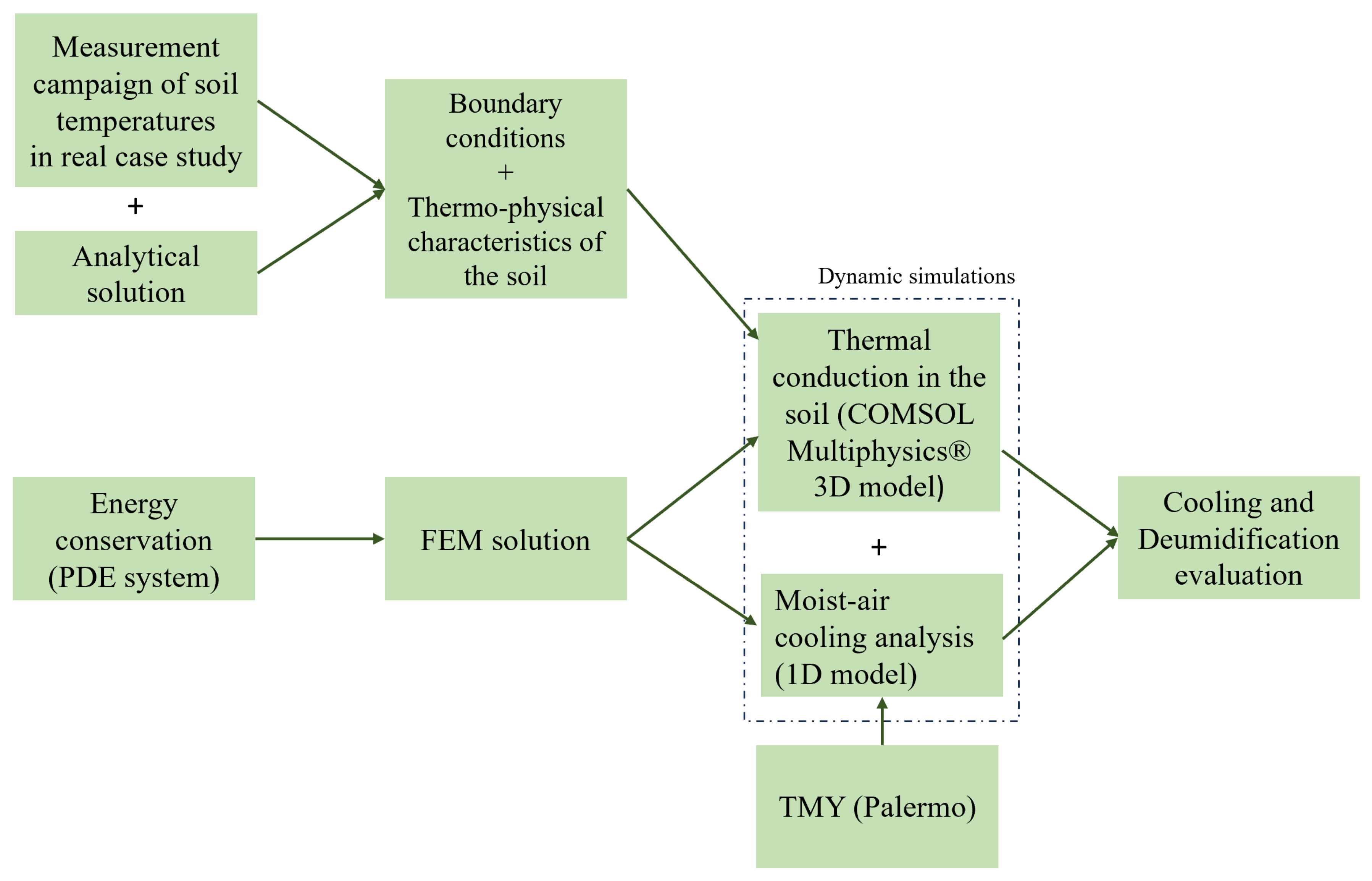
2. Methodology
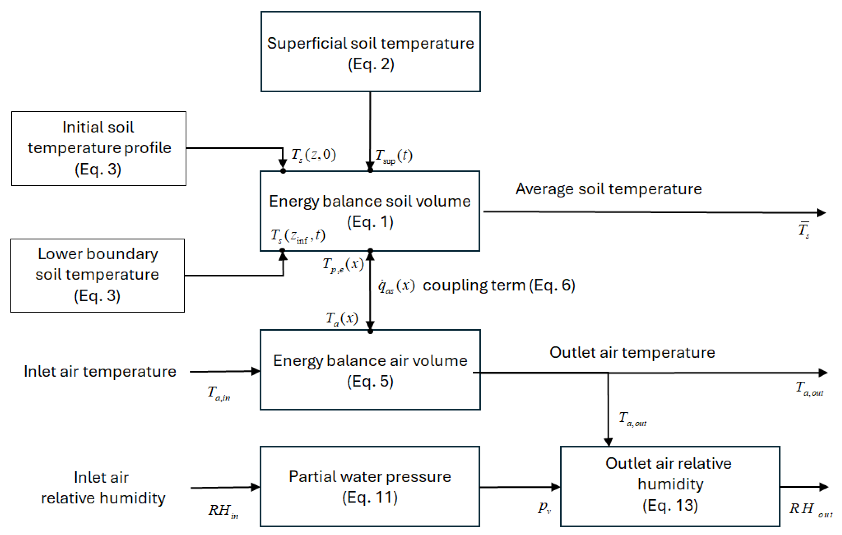
2.1. Formulation of the Equations of the New Finite Element Model
2.2. The Proposed System
3. Case Study and Calibration of the Model
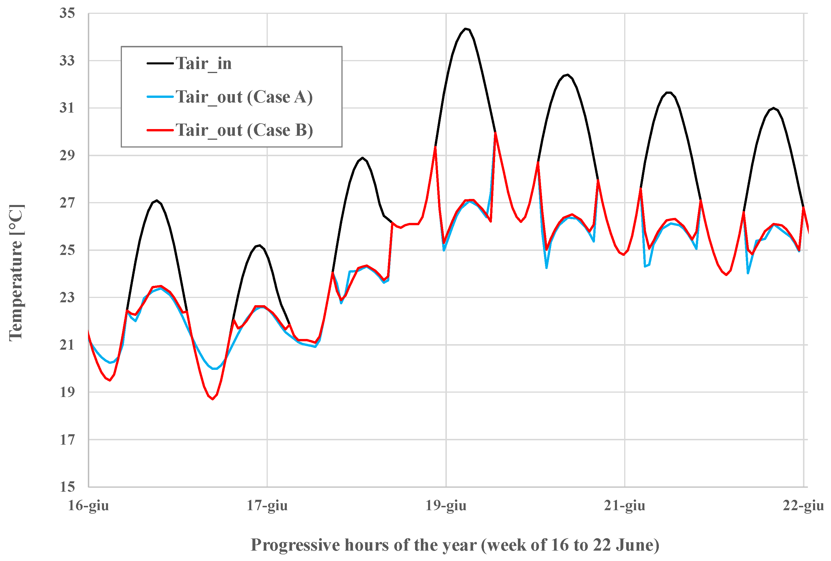
- Case A: during the hours when air conditioning is not operating (between 11 p.m. and 9 a.m.), air is circulated in the exchanger to pre-cool the ground. In this phase, the air leaving the exchanger is rejected into the environment. For the purpose of these analyses, it was assumed that the nightly recirculation of pre-cooled soil air is only active when the outside air temperature is lower than the internal pipe temperatures at the duct inlet.
- Case B: no air is circulated in the heat exchanger during non-conditioning periods.
4. Results and Discussion
5. Analysis of Geothermal Model Integrated with Peltier Cells
6. Conclusions
Author Contributions
Funding
Data Availability Statement
Conflicts of Interest
Abbreviations
| internal cross-sectional area of the pipe [m2] | |
| amplitude of the sinusoid [K] | |
| specific heat of moist air [J·kg−1·K−1] | |
| volumetric heat capacity of the soil [J·m−3·K−1] | |
| time expressed in days | |
| time-lag constant [days] | |
| diameter, [m] | |
| convective heat transfer coefficient [K·m·W−1] | |
| mass flow rate [kg·s−1] | |
| Nusselt number | |
| partial vapor pressure [N·m−2] | |
| Prandtl number | |
| heat flux per unit length [W·m−1] | |
| equivalent thermal resistance [K·m·W−1] | |
| Reynolds number | |
| relative humidity of the air | |
| time, [s] | |
| temperature [K] | |
| annual average value of the air temperature [K] | |
| horizontal coordinate along the pipe [m] | |
| vertical coordinate [m] | |
| Greek letters | |
| thermal diffusivity of soil [m2·s−1] | |
| dumping constant, [m−1] | |
| thermal conductivity [W·m−1·K−1] | |
| density [kg·m−3] | |
| period of the sinusoid, [s] | |
| pulsation [day−1] | |
| friction factor | |
| Subscripts | |
| air | |
| air-to-soil | |
| air-to-pipe | |
| dew point | |
| inner | |
| inlet | |
| inferior | |
| outer | |
| outlet | |
| pipe | |
| pipe-to-soil | |
| Acronyms | |
| BHE | Borehole Heat Exchanger |
| EAHXs | Earth-to-Air Heat eXchanger system |
| FE | Finite Element |
| PDE | Partial Differential Equation |
| PE | cross-linked polyethylene |
| TMY | Typical Metereological Year |
| TRT | Thermal Response Test |
References
- Gondal, I.A.; Masood, S.A.; Amjad, M. Review of geothermal energy development efforts in Pakistan and way forward. Renew. Sustain. Energy Rev. 2017, 71, 687–696. [Google Scholar] [CrossRef]
- Khan, A.; Bradshaw, C.R. Quantitative comparison of the performance of vapor compression cycles with compressor vapor or liquid injection. Int. J. Refrig. 2023, 154, 386–394. [Google Scholar] [CrossRef]
- Ghosal, M.K.; Tiwari, G.N. Modeling and parametric studies for thermal performance of an earth to air heat exchanger integrated with a greenhouse. Energy Convers. Manag. 2006, 47, 1779–1798. [Google Scholar] [CrossRef]
- Congedo, P.M.; Baglivo, C.; Bonuso, S.; D’Agostino, D. Numerical and experimental analysis of the energy performance of an air-source heat pump (ASHP) coupled with a horizontal earth-to-air heat exchanger (EAHX) in different climates. Geothermics 2020, 87, 101845. [Google Scholar] [CrossRef]
- Vaz, J.; Sattler, M.A.; Brum, R.S.; dos Santos, E.D.; Isoldi, L.A. An experimental study on the use of Earth-Air Heat Exchangers (EAHE). Energy Build. 2014, 72, 122–131. [Google Scholar] [CrossRef]
- Cao, S.; Li, F.; Li, X.; Yang, B. Feasibility analysis of Earth-Air Heat Exchanger (EAHE) in a sports and culture center in Tianjin, China. Case Stud. Therm. Eng. 2021, 26, 101054. [Google Scholar] [CrossRef]
- Yang, J.; Song, W.; Zhang, H.; Wang, J.; Dong, J. Experimental study on the characteristics of radiation floor cooling system based on an earth–air heat exchanger. Energy Build. 2023, 296, 113338. [Google Scholar] [CrossRef]
- Bonuso, S.; Panico, S.; Baglivo, C.; Mazzeo, D.; Matera, N.; Congedo, P.M.; Oliveti, G. Dynamic Analysis of the Natural and Mechanical Ventilation of a Solar Greenhouse by Coupling Controlled Mechanical Ventilation (CMV) with an Earth-to-Air Heat Exchanger (EAHX). Energies 2020, 13, 3676. [Google Scholar] [CrossRef]
- Salhein, K.; Kobus, C.J.; Zohdy, M.; Annekaa, A.M.; Alhawsawi, E.Y.; Salheen, S.A. Heat Transfer Performance Factors in a Vertical Ground Heat Exchanger for a Geothermal Heat Pump System. Energies 2024, 17, 5003. [Google Scholar] [CrossRef]
- Luo, M.; Gan, G. Numerical investigation into the thermal interference of slinky ground heat exchangers. Appl. Therm. Eng. 2024, 248, 123215. [Google Scholar] [CrossRef]
- Baglivo, C.; Bonuso, S.; Congedo, P.M. Performance Analysis of Air Cooled Heat Pump Coupled with Horizontal Air Ground Heat Exchanger in the Mediterranean Climate. Energies 2018, 11, 2704. [Google Scholar] [CrossRef]
- Sehli, A.; Hasni, A.; Tamali, M. The Potential of Earth-air Heat Exchangers for Low Energy Cooling of Buildings in South Algeria. Energy Procedia 2012, 18, 496–506. [Google Scholar] [CrossRef]
- Al-Ajmi, F.; Loveday, D.L.; Hanby, V.I. The cooling potential of earth–air heat exchangers for domestic buildings in a desert climate. Build. Environ. 2006, 41, 235–244. [Google Scholar] [CrossRef]
- Hollmuller, P.; Lachal, B. Cooling and preheating with buried pipe systems: Monitoring, simulation and economic aspects. Energy Build. 2001, 33, 509–518. [Google Scholar] [CrossRef]
- Zhang, D.; Zhang, J.; Liu, C.; Yan, C.; Ji, J.; An, Z. Performance measurement and configuration optimization based on or-thogonal simulation method of earth-to-air heat exchange system in cold-arid climate. Energy Build. 2024, 308, 114001. [Google Scholar] [CrossRef]
- Zhou, K.; Mao, J.; Li, Y.; Zhang, H. Performance assessment and techno-economic optimization of ground source heat pump for residential heating and cooling: A case study of Nanjing, China. Sustain. Energy Technol. Assess. 2020, 40, 100782. [Google Scholar] [CrossRef]
- Zhao, Y.; Li, R.; Ji, C.; Huan, C.; Zhang, B.; Liu, L. Parametric study and design of an earth-air heat exchanger using model experiment for memorial heating and cooling. Appl. Therm. Eng. 2019, 148, 838–845. [Google Scholar] [CrossRef]
- Niu, F.; Yu, Y.; Yu, D.; Li, H. Heat and mass transfer performance analysis and cooling capacity prediction of earth to air heat exchanger. Appl. Energy 2015, 137, 211–221. [Google Scholar] [CrossRef]
- Kumar Agrawal, K.; Misra, R.; Das Agrawal, G. To study the effect of different parameters on the thermal performance of ground-air heat exchanger system: In situ measurement. Renew. Energy 2020, 146, 2070–2083. [Google Scholar] [CrossRef]
- Sakhri, N.; Menni, Y.; Ameur, H. Effect of the pipe material and burying depth on the thermal efficiency of earth-to-air heat exchangers. Case Stud. Chem. Environ. Eng. 2020, 2, 100013. [Google Scholar] [CrossRef]
- Alqawasmeh, Q.I.; Narsilio, G.A.; Makasis, N. Impact of geometrical misplacement of heat exchanger pipe parallel configuration in energy piles. Energies 2024, 17, 2580. [Google Scholar] [CrossRef]
- Zhou, Y.; Bidarmaghz, A.; Makasis, N.; Narsilio, G. Ground-source heat pump systems: The effects of variable trench separations and pipe configurations in horizontal ground heat exchangers. Energies 2021, 14, 3919. [Google Scholar] [CrossRef]
- Cherif Lekhal, M.; Belarbi, R.; Mokhtari, A.M.; Benzaama, M.-H.; Bennacer, R. Thermal performance of a residential house equipped with a combined system: A direct solar floor and an earth–air heat exchanger. Sustain. Cities Soc. 2018, 40, 534–545. [Google Scholar] [CrossRef]
- Ghiasi, M.; Wang, Z.; Mehrandezh, M.; Paranjape, R. Enhancing efficiency through integration of geothermal and photovoltaic in heating systems of a greenhouse for sustainable agriculture. Sustain. Cities Soc. 2025, 118, 106040. [Google Scholar] [CrossRef]
- Jathunge, C.B.; Dworkin, S.B.; Wemhöner, C.; Mwesigye, A. Performance investigation of a solar-assisted ground source heat pump system coupled with novel offset pipe energy piles and solar PVT collectors for cold climate applications. Appl. Therm. Eng. 2025, 265, 125568. [Google Scholar] [CrossRef]
- Shahsavar, A.; Azimi, N. Performance evaluation and multi-objective optimization of a hybrid earth-air heat exchanger and building-integrated photovoltaic/thermal system with phase change material and exhaust air heat recovery. J. Build. Eng. 2024, 90, 109531. [Google Scholar] [CrossRef]
- Bhutta, M.M.A.; Hayat, N.; Bashir, H.M.; Khan, A.R.; Ahmad, K.N.; Khan, S. CFD applications in various heat exchangers design: A review. Appl. Therm. Eng. 2012, 32, 1–12. [Google Scholar] [CrossRef]
- Congedo, P.M.; Lorusso, C.; Baglivo, C.; Milanese, M.; Raimondo, L. Experimental validation of horizontal air-ground heat exchangers (HAGHE) for ventilation systems. Geothermics 2019, 80, 78–85. [Google Scholar] [CrossRef]
- Li, C.; Jiang, C.; Guan, Y.; Chen, K.; Wu, J.; Xu, J.; Wang, J. Simplified method and numerical simulation analysis of pipe-group long-term heat transfer in deep-ground heat exchangers. Energy 2024, 299, 131533. [Google Scholar] [CrossRef]
- Buscemi, A.; Beccali, M.; Guarino, S.; Lo Brano, V. Coupling a road solar thermal collector and borehole thermal energy storage for building heating: First experimental and numerical results. Energy Convers. Manag. 2024, 291, 117279. [Google Scholar] [CrossRef]
- Incropera, F.P.; DeWitt, D.P.; Bergman, T.L.; Lavine, A.S. Fundamentals of Heat and Mass Transfer 5th Edition with IHT2.0/FEHT with Users Guides; Wiley: Hoboken, NJ, USA, 2001. [Google Scholar]
- Gnielinski, V. On heat transfer in tubes. Int. J. Heat Mass Transf. 2013, 63, 134–140. [Google Scholar] [CrossRef]
- Tsilingiris, P.T. Thermophysical and transport properties of humid air at temperature range between 0 and 100 °C. Energy Convers. Manag. 2008, 49, 1098–1110. [Google Scholar] [CrossRef]
- Gatley, D.P. Understanding Psychrometrics, 3rd ed.; The American Society of Heating, Refrigerating and Air-Conditioning Engineers, Inc.: Atlanta, GA, USA, 2013. [Google Scholar]
- Congedo, P.M.; Baglivo, C.; Negro, G. A New Device Hypothesis for Water Extraction from Air and Basic Air Condition System in Developing Countries. Energies 2021, 14, 4507. [Google Scholar] [CrossRef]


| T0 [°C] | B [°C] | d* [day] | τ [day] | ω [1/day] | γ [1/m] |
|---|---|---|---|---|---|
| 22.36 | 13.50 | 147.19 | 365 | 0.017214 | 0.379117 |
Disclaimer/Publisher’s Note: The statements, opinions and data contained in all publications are solely those of the individual author(s) and contributor(s) and not of MDPI and/or the editor(s). MDPI and/or the editor(s) disclaim responsibility for any injury to people or property resulting from any ideas, methods, instructions or products referred to in the content. |
© 2025 by the authors. Licensee MDPI, Basel, Switzerland. This article is an open access article distributed under the terms and conditions of the Creative Commons Attribution (CC BY) license (https://creativecommons.org/licenses/by/4.0/).
Share and Cite
Baglivo, C.; Buscemi, A.; Spagnolo, M.; Bonomolo, M.; Lo Brano, V.; Congedo, P.M. Toward a Sustainable Indoor Environment: Coupling Geothermal Cooling with Water Recovery Through EAHX Systems. Energies 2025, 18, 2297. https://doi.org/10.3390/en18092297
Baglivo C, Buscemi A, Spagnolo M, Bonomolo M, Lo Brano V, Congedo PM. Toward a Sustainable Indoor Environment: Coupling Geothermal Cooling with Water Recovery Through EAHX Systems. Energies. 2025; 18(9):2297. https://doi.org/10.3390/en18092297
Chicago/Turabian StyleBaglivo, Cristina, Alessandro Buscemi, Michele Spagnolo, Marina Bonomolo, Valerio Lo Brano, and Paolo Maria Congedo. 2025. "Toward a Sustainable Indoor Environment: Coupling Geothermal Cooling with Water Recovery Through EAHX Systems" Energies 18, no. 9: 2297. https://doi.org/10.3390/en18092297
APA StyleBaglivo, C., Buscemi, A., Spagnolo, M., Bonomolo, M., Lo Brano, V., & Congedo, P. M. (2025). Toward a Sustainable Indoor Environment: Coupling Geothermal Cooling with Water Recovery Through EAHX Systems. Energies, 18(9), 2297. https://doi.org/10.3390/en18092297