Transformers and Long Short-Term Memory Transfer Learning for GenIV Reactor Temperature Time Series Forecasting

Abstract

Automated monitoring of the coolant temperature can enable autonomous operation of generation IV reactors (GenIV), thus reducing their operating and maintenance costs. Automation can be accomplished with machine learning (ML) models trained on historical sensor data. However, the performance of ML usually depends on the availability of large amount of training data, which is difficult to obtain for GenIV, as this technology is still under development. We propose the use of transfer learning (TL), which involves utilizing knowledge across different domains, to compensate for this lack of training data. TL can be used to create pre-trained ML models with data from small-scale research facilities, which can then be fine-tuned to monitor GenIV reactors. In this work, we develop pre-trained Transformer and long short-term memory (LSTM) networks by training them on temperature measurements from thermal hydraulic flow loops operating with water and Galinstan fluids at room temperature at Argonne National Laboratory. The pre-trained models are then fine-tuned and re-trained with minimal additional data to perform predictions of the time series of high temperature measurements obtained from the Engineering Test Unit (ETU) at Kairos Power. The performance of the LSTM and Transformer networks is investigated by varying the size of the lookback window and forecast horizon. The results of this study show that LSTM networks have lower prediction errors than Transformers, but LSTM errors increase more rapidly with increasing lookback window size and forecast horizon compared to the Transformer errors.

1. Introduction

Generation IV (GenIV) advanced nuclear reactors, such as molten salt-cooled, liquid metal-cooled, and gas-cooled reactors, are potentially promising options to replace the aging fleet of commercial light water reactors [1,2]. The economic viability of GenIV reactors depends on low operating and maintenance (O&M) costs, which can potentially be achieved through autonomous operation and predictive maintenance [3,4,5]. Reactor operations involve the monitoring of process coolant variables, such as temperature, flow rate, and pressure. Coolant temperature sensing is one of the most common types of measurements in reactor systems because this provides real-time information about reactor power [6]. Temperature measurements in nuclear reactors are typically made with thermocouple sensors, which are a preferable option because of their compatibility with operating conditions, resilience to harsh environment, and relatively low cost [7]. Thermocouples consist of chromel (nickel-chromium alloy) and alumel (nickel-aluminum alloy) wires joined at one end. Voltage across the junction is proportional to the temperature. Nuclear grade type-K thermocouples are designed to withstand temperatures ranging from −200 °C to 1372 °C. However, exposure to high temperatures and corrosive fluids in GenIV reactors can pose significant challenges to the long-term reliability and accuracy of measurements. The lifetime of thermocouples is limited by material degradation due to thermal stresses, ionizing radiation, and corrosion. Over time, these effects can lead to drift in temperature readings, reduced accuracy, and sensor failure [8].

Automation of temperature sensor fault detection can be achieved through sensor time series monitoring with statistical methods [9,10,11,12,13] and machine learning (ML) techniques [13,14,15,16,17,18,19,20,21]. Recent work on statistical methods for nuclear reactor sensor time series analysis has included the principal component analysis (PCA) [9], least squares [9], independent component analysis (ICA) [9], singular value decomposition (SVD) [10,11], likelihood ratio test (LRT) [10], moving average filter [12], and the autoregressive integrated moving average (ARIMA) [13] methods. Recent work on ML models for nuclear reactor sensor time series has included Long-Short-Term-Memory (LSTM) [13,14,15,16], convolutional neural networks (CNNs) [14,15], Gated Recurrent Units (GRUs) [15,17], a combination of CNNs with LSTM [15], convolutional LSTM networks combined with Kullback-Leibler divergence [18], deep belief networks (DBNs) and LRTs [19], CNNs with attention mechanism [20], and Transformers [21,22,23,24]. The focus of our work is on benchmarking the performance of LSTMs that have recurrent network mechanisms, and Transformers that have the attention mechanism, making these networks particularly efficient in capturing long-term dependencies in time series.

ML methods have the advantage of performing data-agnostic analysis that is efficient at processing nonlinear data and do not require data preprocessing [13]. However, the development of ML models that achieve reasonably low forecasting errors requires extensive training on a large amount of historical sensor measurements to capture variance of the normal operating data [13,25]. Historical training data are limited because GenIV facilities are still under development, and running high temperature facilities to generate training data is relatively expensive. Our proposed approach to overcome the lack of training data involves using the Transfer Learning (TL) concept by leveraging training data from relatively low-cost room temperature experimental facilities. TL involves pre-training ML models on some databases and then adapting them to applications in different domains with minimal ML model re-training [26,27,28,29]. Our proposed approach to training ML models to monitor GenIV reactors parallels a common strategy in proof-of-concept thermal hydraulic experiments of using surrogate fluids at room temperatures as lower cost alternatives to high temperature fluids [30].

In this paper, LSTM and Transformers are trained on data from type-K thermocouple sensor measurements in test flow loops, where the process fluids are water and Galinstan in the temperature range of 20 °C to 60 °C. These ML models are then used to forecast temperature measurements made with type-K thermocouples in a different facility, where the working fluid is Argon gas in a temperature range from 300 °C to 500 °C. The performance of LSTM and Transformers models is investigated under varying lookback windows and forecast horizon lengths. The study of the lookback window sizes aims to determine the values that minimize errors in forecasting. The study of the forecast horizon aims to maximize the forecast horizon length for anticipation of events, subject to the constraint of minimizing forecasting errors. The performance of the models is evaluated by calculating the root mean squared error (RMSE) and maximum absolute error (MaxAE) of the predictions. The results of this study show that LSTM have lower prediction errors than Transformers, but LSTM errors increase more rapidly with increasing lookback window size and increasing forecast horizon compared to the Transformers errors.

This paper is organized as follows. Section 2 describes the ML models and approaches used in this work. Section 3 describes data acquisition and pre-processing. Section 4 includes the ML methodology, including pre-training and fine-tuning of the ML models. Section 5 presents the results of LSTM and Transformers forecasting error dependence on the lookback window and forecast horizon size. Section 6 concludes the paper.

2. Machine Learning Models

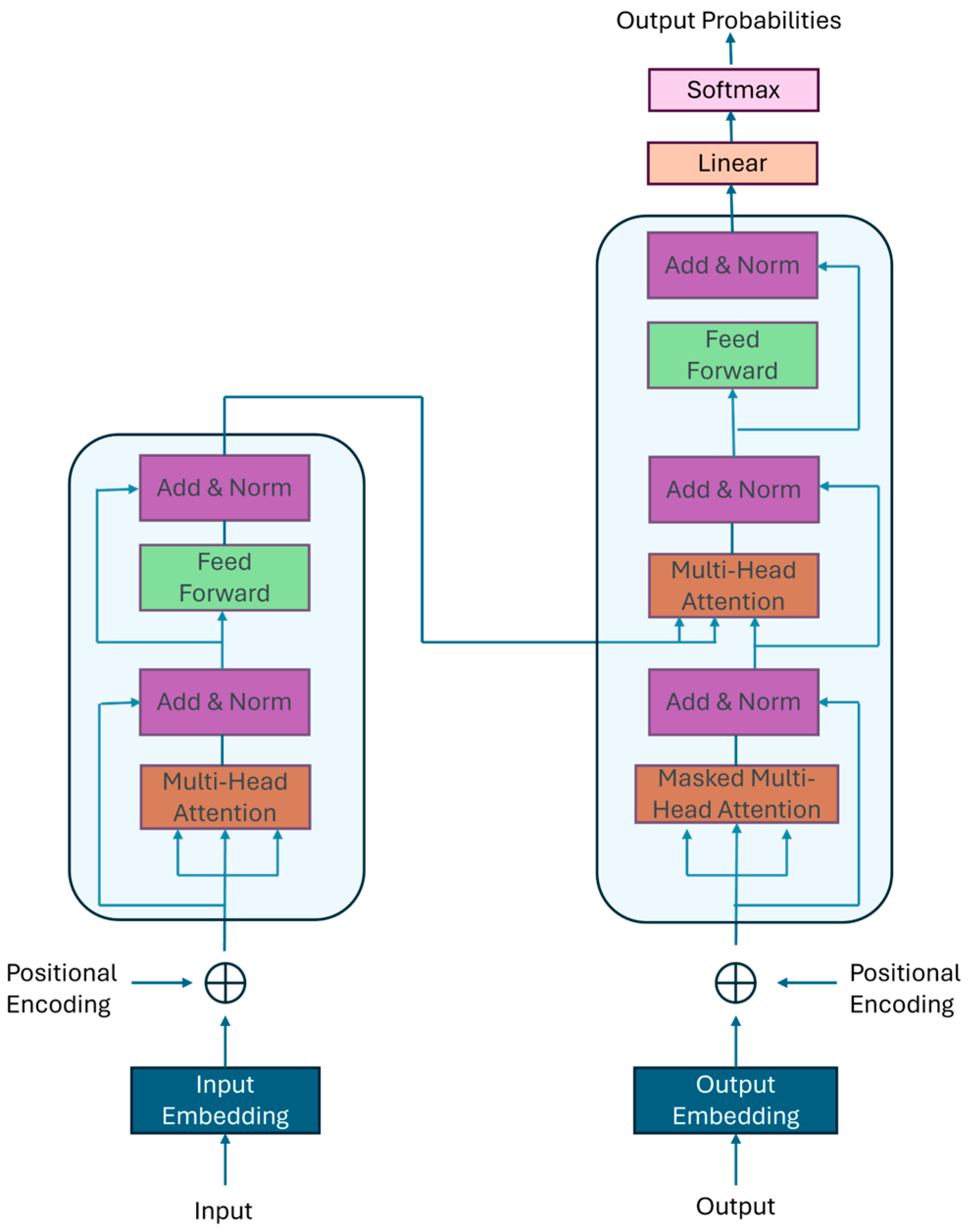
2.1. Transformers

Transformers are one of the architectures for the implementation of foundation models (FM). Transformers were initially developed for applications in natural language processing (NLP) tasks to process large amounts of text while capturing complex patterns and dependencies in the language. Transformers depend on self-attention, a mechanism that allows them to process input sequences in parallel, rather than sequentially, which allows for more efficient handling of long-term dependencies [21,22,23,24,31,32]. This is particularly important in natural language data, where the relationships between words must be understood, regardless of their position in sentences. The self-attention mechanism creates attention weights that measure the relevance between parts of the input. These weights are calculated through three components derived from the input data: the query (Q), which represents the current data point being evaluated; the key (K), which represents all other data points; and the value (V), which contains the information needed from each data point. Similarity scores are calculated by computing the relationships between Q and each K and then normalized to form attention weights. The model tends to assign higher weights to relevant data and lower weights to less important data. The attention function is calculated as shown in Equation (1), where d_k represents a scaling factor that is used to counteract possible issues related to very small gradients stemming from the softmax activation function:

$$attention\left(Q,K,V\right)=softmax\left({\displaystyle \frac{Q{K}^T}{\surd d_k}}\right)V$$

(1)

To further enhance this ability, Transformers use multi-head attention, in which the self-attention mechanism is applied multiple times (in “heads”), where each head focuses on different parts or features of the data:

$$hea{d}_i=attention\left(Q{W}_i^Q,K{W}_i^K,V{W}_i^V\right)$$

(2)

Each head implements the attention function from Equation (1), characterized by projection weights $W_i^Q$, $W_i^K$, and $W_i^V$, for query, key, and value, respectively. The combined results from all heads allow for a more comprehensive capture of various input patterns. The multi-head attention function is expressed as:

$$multihead\left(Q,K,V\right)=concat\left(hea{d}_1,\dots ,hea{d}_h\right)W^o$$

(3)

where all heads are concatenated and scaled by weight matrix $W^o$. The weights $W_i^Q,W_i^K,W_i^V,\mathrm{a}\mathrm{n}\mathrm{d}{W}^o$ in Equations (2) and (3) are optimized using the mean squared error (MSE) loss function, and the gradients used to update the weights are calculated using backpropagation.

In contrast to traditional recurrent neural networks (RNN), Transformers process all points in a sequence simultaneously, by transforming sequence points into vectors, called embeddings. Even though this parallel processing is computationally efficient, Transformers are unaware of the relative position of points in a sequence. The positional encoding mechanism provides the Transformer with this information. The encodings are vectors added to the embeddings of sequence points that are unique for each position, with the objective being to differentiate among different positions. Sinusoidal functions are a frequently used method to create positional encodings. For a given position (p) in a sequence and a dimension (d) of an embedding, the encoding is calculated for each dimension index (i) as follows:

$$PE\left(p,2i\right)=\mathrm{s}\mathrm{i}\mathrm{n}\left({\displaystyle \frac{p}{{10000}^{2i/d}}}\right)$$

(4)

$$PE\left(p,2i+1\right)=\mathrm{c}\mathrm{o}\mathrm{s}\left({\displaystyle \frac{p}{{10000}^{2i/d}}}\right)$$

(5)

The encoding values are in the range [−1, 1], and they are compatible with the value ranges of the embeddings.

A schematic diagram of the Transformer network architecture is shown in Figure 1. The encoder consisting of N layers is on the left side of the diagram. Each layer of the encoder consists of a multi-head self-attention mechanism and a fully connected feed forward network. Each of these sublayers is followed by an Add & Norm sublayer, which produces the output Norm(x + Sublayer(x)), where Sublayer(x) is the output from each sublayer. The decoder consisting of N layers is on the right part of the diagram in Figure 1. The structure of the decoder includes the same sublayers as those in the encoder. In addition, the decoder includes a third sublayer, which performs the multi-head attention operation on the output produced by the encoder. The masked multi-head attention ensures that predictions depend only on the outputs in preceding positions. This is accomplished by setting the input values of the softmax layer accordingly (see Equation (1)).

2.2. Long Short-Term Memory (LSTM) Networks

In this study, long short-term memory (LSTM) networks are used to benchmark the performance of the Transformers. LSTM networks are a special type of RNN designed to handle sequential data while overcoming the limitations of traditional RNN [13,14,15,16]. Standard RNNs struggle to capture long-term dependencies due to vanishing and exploding gradients. LSTM networks have the ability to selectively retain or discard information over time. An LSTM cell consists of an Input gate, a Forget gate, and an Output gate, which regulate the flow of information. The Forget gate decides which information to discard from the cell state, the Input gate determines which new information to add, and the Output gate controls which part of the cell state becomes the output. These gates rely on learned parameters that are updated during training, allowing the network to adapt to the specifics of the application domain data. The gating mechanism gives LSTM the ability to remember patterns over extended sequences, which makes them well-suited for tasks that involve time series data, natural language processing, and other sequential data challenges. For each time step, the LSTM cell calculates hidden state H_t and current state C_t according to:

$$H_t=\sigma (x_t{U}_o+H_{t-1}{W}_o)\mathrm{t}\mathrm{a}\mathrm{n}\mathrm{h}\left(C_t\right)$$

(6)

$$C_t=\sigma \left(x_t{U}_f+H_{t-1}{W}_f\right)C_{t-1}+\sigma (x_t{U}_i+H_{t-1}{W}_i)\mathrm{t}\mathrm{a}\mathrm{n}\mathrm{h}(x_t{U}_c+H_{t-1}{W}_c)$$

(7)

where x is the input to the cell, U and W represent weight matrices, and the indices i, o, f, refer to Input, Output and Forget gates, respectively. Finally, σ is the sigmoid gating activation function, and tanh is the output activation function. The LSTM weights U_o, U_i, U_f, U_c, W_o, W_i, W_f, and W_c in Equations (6) and (7) are optimized using the MSE loss function. Gradients that are used to update the weights in LSTM networks are computed recursively using the backpropagation through time (BPTT) algorithm, which accumulates gradients over multiple time steps.

2.3. Transfer Learning (TL)

Transfer learning (TL) refers to the concept of knowledge transfer between a source (S) and a target (T) domain. Let $X_S$ be the n historical observations of a time series in the input, and $Y_S$ be the m + 1 future observations of the time series in the output of domain S:

$$X_S=\{X_S\left(t-n\right),\dots ,X_s\left(t-1\right)\}$$

(8)

$$Y_S=\{X_S\left(t\right),\dots ,X_s\left(t+m\right)\}$$

(9)

Similarly, we define $X_T$ to be the n historical observations in the input, and $Y_T$ to be m + 1 future observations of a time series in the output of domain T:

$$X_T=\{X_T\left(t-n\right),\dots ,X_T\left(t-1\right)\}$$

(10)

$$Y_T=\{X_T\left(t\right),\dots ,X_T\left(t+m\right)\}$$

(11)

The goal of TL is to transfer knowledge obtained by training a model on domain S to improve the model’s performance in forecasting on domain T. The prediction model in this case can be expressed as

$$\widehat{Y_T}=f_T(f_S\left(X_T;{\theta }_S\right),{\theta }_T)$$

(12)

where f_S is the learning function and θ_S are parameters obtained by training a model on data from domain S. Function f_S and the respective parameters θ_S are transferred when the pre-trained model is fine-tuned with data from domain T. Re-training of the model on data from domain T creates new learning function f_T and training parameters θ_T.

3. Temperature Data Acquisition and Conditioning

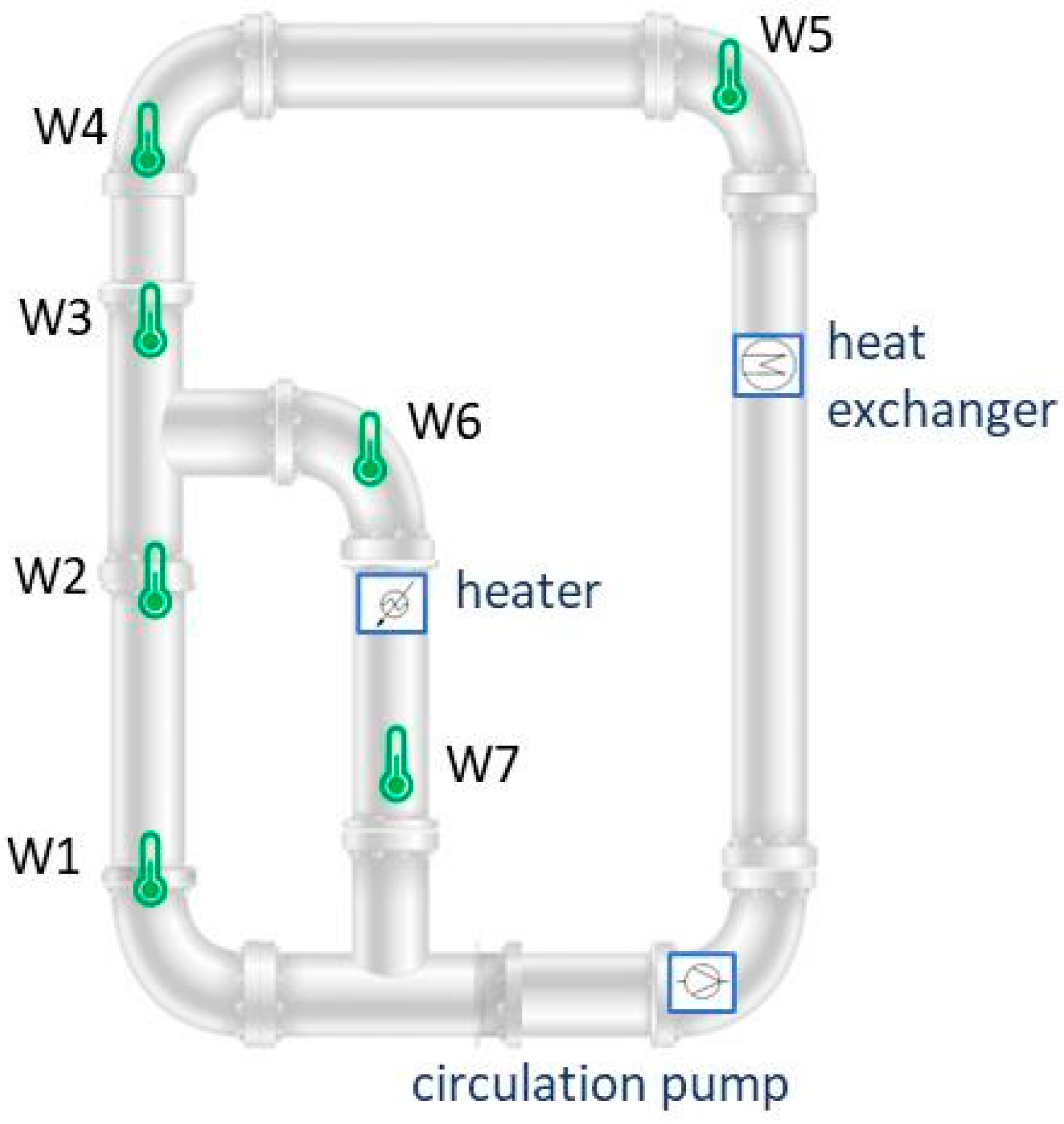
3.1. Measurements in Room Temperature Flow Loops

High temperature thermal hydraulics research facilities frequently utilize experimental setups with room-temperature surrogate fluids to perform preliminary proof-of-principle studies or to test equipment [33]. Water and Galinstan are examples of room temperature, chemically inert fluids that have similar density and thermal conductivity to liquid sodium, respectively. Galinstan is a eutectic alloy of gallium, indium, and tin, with a low melting point (around −19 °C) at ambient pressure.

In our study, water and Galinstan temperature measurements were obtained from a thermal hydraulic test loop with a mixing thermal Tee at Argonne National Laboratory. The flow loop is equipped with seven type-K thermocouple sensors (labeled W1 to W7 in water and G1 to G7 in Galinstan) [13,16,33]. The loop is constructed from polycarbonate piping which can operate within a temperature range of 0 °C to 121 °C. In one experiment, water was used as the working fluid, while in another, the loop was filled with liquid metal Galinstan. A variable-speed 1.5 HP stainless steel pump circulated the fluid clockwise through the loop against gravity. The main loop was divided into “hot leg” and “cold leg” sections. The fluid in the “hot leg” was heated by a variable-power Watlow FLC-16 heater with a maximum output of 4 kWe. After heating, the “hot leg” fluid mixed with the “cold leg” stream in a thermal Tee junction. The pipe diameters for the “hot leg” and “cold leg” were 1.9 cm and 3.81 cm, respectively. Following the mixing process, the fluid was cooled back to room temperature using a 130,000 BTU Shell & Tube heat exchanger connected to a chiller with an 11,300 BTU/h capacity.

A schematic of the water-filled flow loop with placements of thermocouples W1 through W7 is shown in Figure 2. An identical configuration was set up for the Galinstan-filled flow loop to obtain measurements with thermocouples G1 through G7.

Sensor readings were logged using a LabVIEW™ 2019-integrated data acquisition system. The average temperatures of the seven thermocouples recorded during the experiment in the water and Galinstan loops are shown in

Table 1. Average temperatures of thermocouples in room temperature flow loop.

Water Loop		Galinstan Loop
Thermocouple Label	Average Temperature (°C)	Thermocouple Label	Average Temperature (°C)
W1	30	G1	24
W2	30	G2	24
W3	32	G3	26
W4	32	G4	26
W5	32	G5	26
W6	37	G6	39
W7	52	G7	33

. The time series from the thermocouples in water and in Galinstan are 2100 s-long and 1470 s-long, respectively. The uncertainty in measurements is max(0.75%, 2.2 °C).

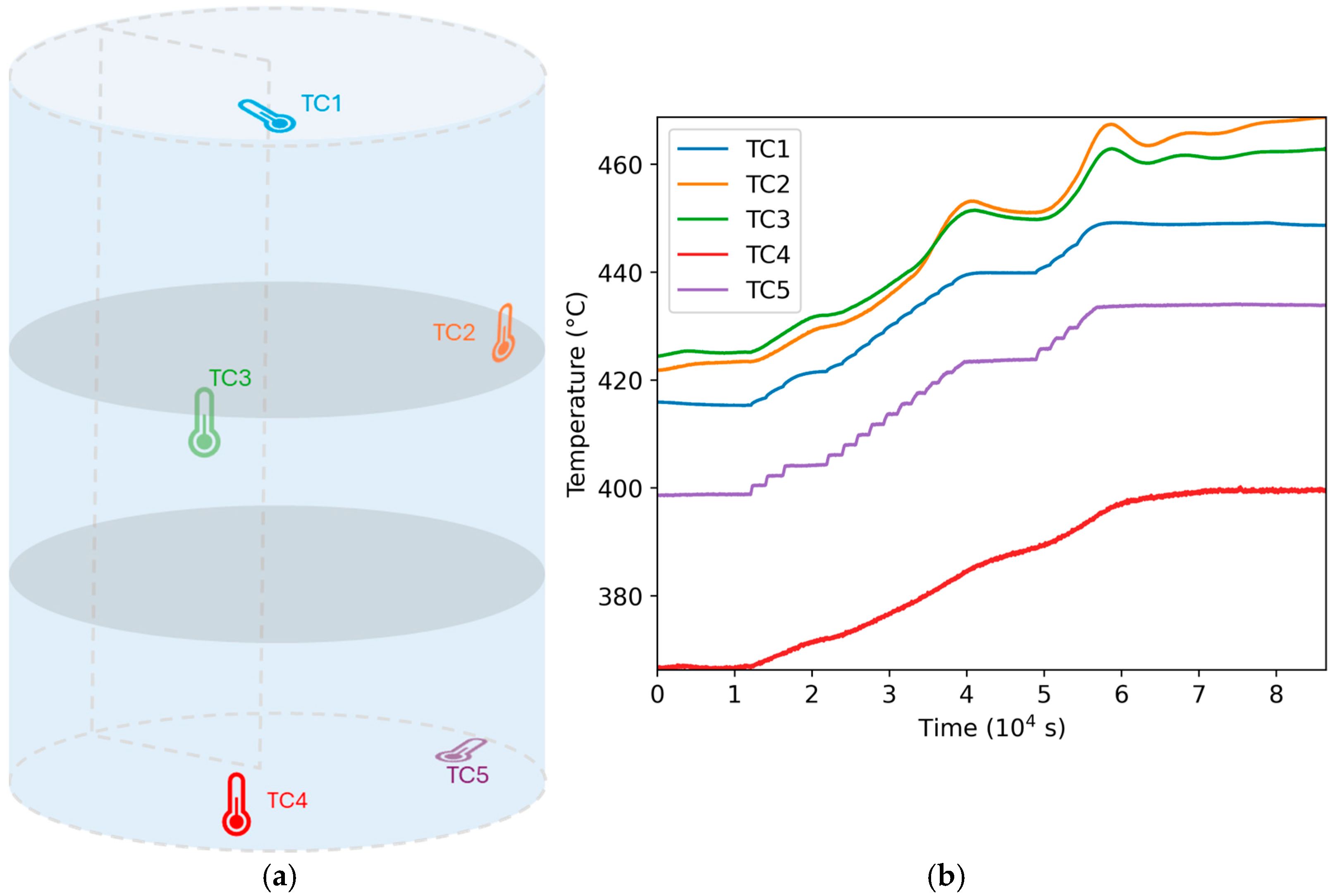
3.2. Measurements in High Temperature Vessel

Argon gas measurements were obtained from thermocouple sensors installed in the vessel of the Kairos Power Engineering Test Unit (ETU) during a heat-up transient of the vessel [34]. Although the ETU is developed for molten salt thermal hydraulic experiments, the vessel heat-up test was conducted using inert argon gas as the fluid. The vessel is split into five distinct zones, labeled as Z1 to Z5, which are monitored with type-K thermocouples. There are 15 thermocouples in the top zone Z1, 17 thermocouples in the bottom zone Z5, 11 thermocouples in the upper part of the vessel side zone Z2, 12 thermocouples in the middle part of the vessel side zone Z3, and 12 thermocouples in the lower part of the vessel side zone Z4. The data acquisition system (DAQ) of ETU recorded a measurement every time a change in temperature was detected, thus making the measurement resolution non-uniform. To achieve a uniform measurement resolution of 1 s, any missing values between recorded measurements were padded with the respective last recorded values. The total length of all thermocouple time series after padding is 86,418 s.

One thermocouple from each vessel zone was selected in this study according to the procedure described in Section 3.3. The average values of temperature measured with thermocouples TC1 to TC5 are listed in

Table 2. Average temperatures of ETU vessel thermocouples.

ETU Vessel Thermocouple	Average Temperature (°C)
TC1	435
TC2	447
TC3	446
TC4	384
TC5	419

. The thermocouples and their positions in the vessel zones are shown in Figure 3a, where TC1 through TC5 are in the respective zones Z1 through Z5. The time series from the five thermocouples in the ETU vessel are shown in Figure 3b.

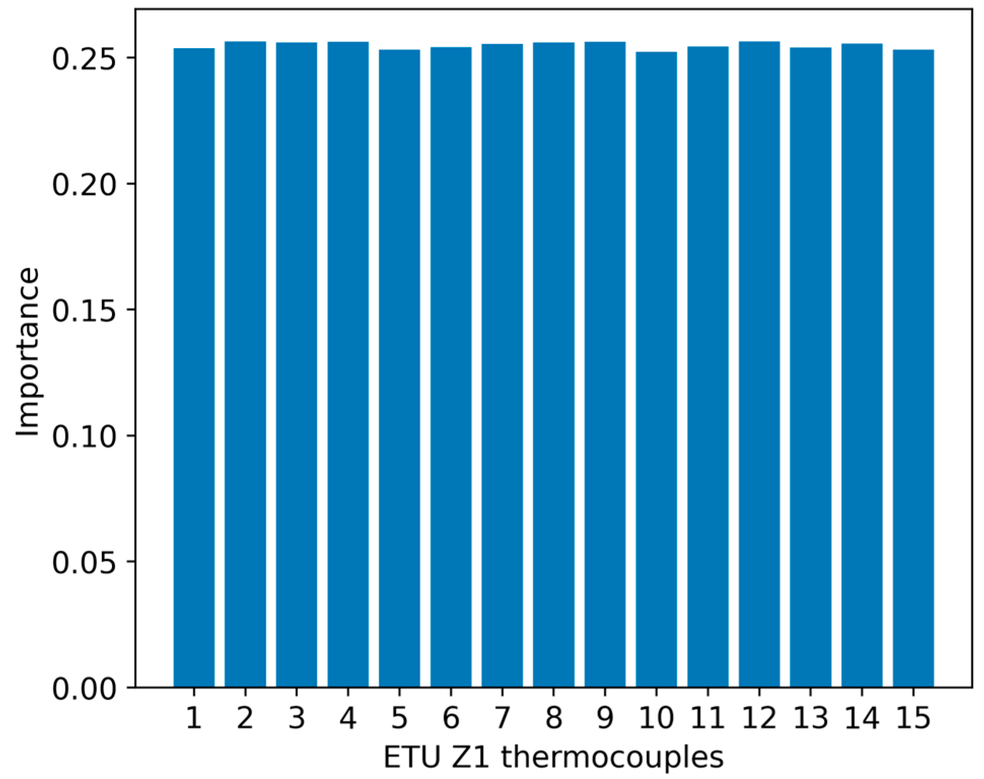
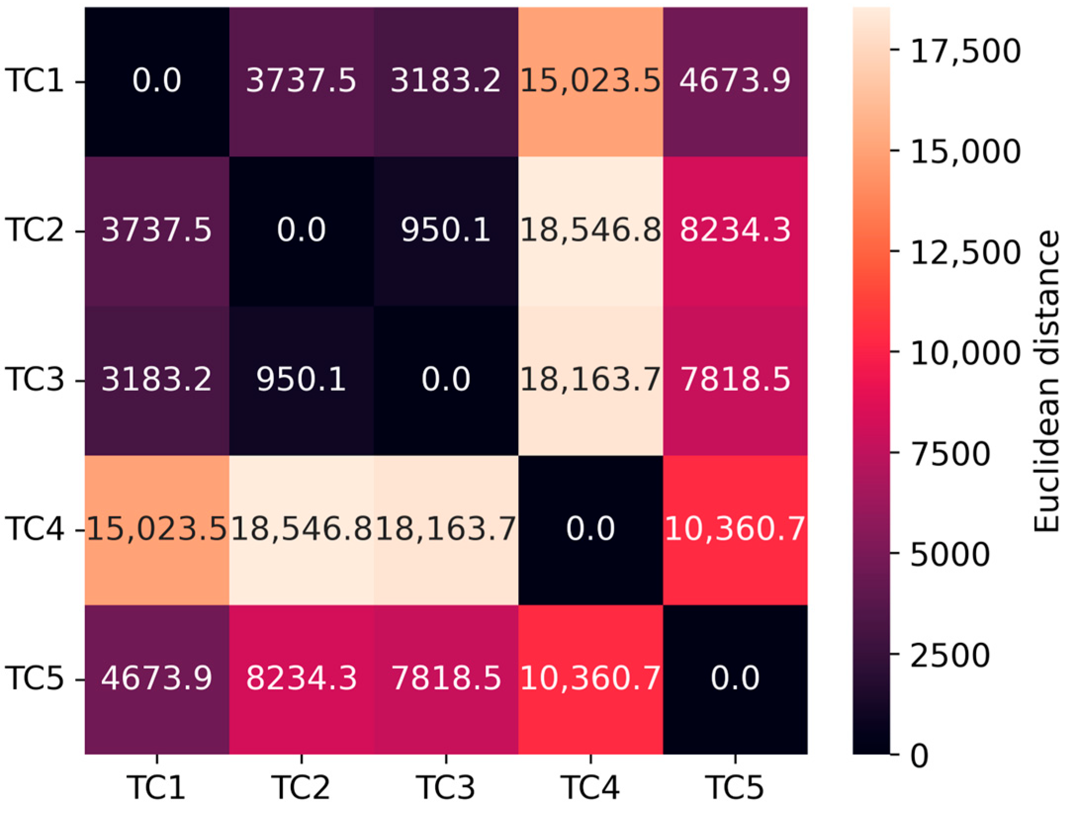
3.3. Selection of Thermocouples from Each Zone in the ETU Vessel

Multiple thermocouples were installed in the same zones of the ETU to achieve redundancy that would allow for continuous test facility operation. An operating commercial reactor will be instrumented with substantially fewer thermocouples. Therefore, to represent the scenario of forecasting temperature measurements in a reactor vessel with a few physical sensor units, we selected one thermocouple sensor from each ETU zone using principal component analysis (PCA) [35]. PCA is frequently used to reduce the dimensionality of large datasets. The PCA algorithm uses statistical procedures to create a set of linearly uncorrelated variables. Identification of correlations between variables in a dataset is achieved through calculation of the covariance matrix C. For n vectors x₁, x₂, …, x_n, C is a n × n matrix in which the elements are covariances between all pairs of vectors:

$$C=\left[\begin{array}{ccc}Cov(x_1,x_1)& \cdots & Cov(x_1,x_n)\\ ⋮& \ddots & ⋮\\ Cov(x_n,x_1)& \cdots & Cov(x_n,x_n)\end{array}\right]$$

(13)

Covariance for vectors x and y of length N, with mean values $\overline{x}$ and $\overline{y}$, respectively, is calculated as:

$$Cov\left(x,y\right)={\displaystyle \frac{\sum (x_i-\overline{x})(y_i-\overline{y})}{N}}$$

(14)

Positive covariance values indicate correlation between vectors, while negative values of covariance indicate an anti-correlation.

Calculating the eigenvectors corresponding to the k largest eigenvalues of C and calculating the outer product with the original data gives k principal components of a dataset. A subset of the principal components is sufficient to represent the same information as the original data. The optimal number of principal components can be determined by calculating the explained variance. The summation of explained variances for all principal components equals 100%. The first principal component has the largest percentage of explained variance. Typically, values of explained variance above 85% are considered sufficient for retaining most of the original data information. For the thermocouple time series data for all vessel zones in ETU, the first principal component had an explained variance close to 100%, as shown in

Table 3. Explained variance values for the first principal component in each of the ETU vessel zones.

ETU Vessel Zone	Explained Variance (%)
Z1	98.72
Z2	99.04
Z3	97.98
Z4	99.65
Z5	99.69

.

The relative importance of features can be ranked by the absolute values of the PCA loadings, which are calculated by multiplying the coefficients of the linear combination of the original variables in the dataset by the explained variance. An example of the relative importance of each of the 15 thermocouples in ETU vessel zone Z1 is shown in Figure 4. The thermocouple with the largest importance was chosen from the set of 15 thermocouples in Z1 and labeled TC1 (see Figure 3a). A similar procedure was followed to select thermocouples from the other four zones of the vessel Z2 through Z5.

3.4. Augmentation of Training Data

Because the length of training data temperature time series in the water and Galinstan flow loops was shorter than the testing data temperature time series in the ETU vessel, we augmented training data using window warping. Window warping involves stretching or compressing data along the time axis to simulate different speeds of data generation [36].

To create additional training data, the time dimension is stretched across the time series. For a time series of the form shown in Equation (15), where each point is associated with time instances t₁, t₂, …t_m, window warping is achieved by adding points between the existing ones using linear interpolation.

$$X=[x_1,x_2,\dots ,x_m]$$

(15)

The number of newly created data points depends on the amount of stretching applied to the time axis. For a factor of stretching equal to d, the interpolated time points between t_i and t_i+1 will be of the form

$$t_n=t_i+{\displaystyle \frac{n}{d}}\left(t_{i+1}-t_i\right),1\le n<d$$

(16)

while the interpolated points of the time series between x_i and x_i+1 will be

$$x_n=x_i+{\displaystyle \frac{n}{d}}\left(x_{i+1}-x_i\right),1\le n<d$$

(17)

Window warping inserts more data points in a time series while preserving the distribution of the data. Augmented training data were created by using window warping with a stretching factor of d = 41 for the water flow loop time series and a stretching factor of d = 59 for the Galinstan time series.

4. Machine Learning Models Implementation

4.1. Training of Forecasting Models

The structure of the LSTM and Transformer networks was developed using grid search optimization. This involved an exhaustive search through the hyperparameter space of the respective networks to choose the combinations of variables that yield the best performance of the network during the validation process.

The Transformers model developed in this work consists of an encoder, which projects input data into a desired dimension, a positional encoding layer, a Transformer encoder layer that processes the data through eight self-attention heads, two linear layers, and a decoder that produces the output. The total number of trainable parameters (weights and biases) is 35,169, which include 8 weights and 8 bias terms in the encoder, 256 weights and 32 bias terms in the Transformer encoder layer, 32,784 weights and 2072 bias terms in the linear layers, and 8 weights and 1 bias term in the decoder layer. The structure of the Transformer was developed by running grid search optimization in the hyperparameter space consisting of the number of self-attention heads in the range (1, 20), and the number of linear layers in the range (1, 5). The learning rate was varied in the range (10⁻⁵, 10⁻³).

The LSTM model in this work consists of an LSTM layer with 16 hidden units, a 10% dropout layer, and two fully connected layers. The total number of trainable parameters (weights and biases) is 1361, which include 1088 weights and 128 bias terms in the LSTM layer and 136 weights and 9 bias terms in the fully connected layers. The variables in the LSTM grid search hyperparameter space consisted of the number of hidden units with the range (1, 100), the number of fully connected layers with the range (1, 3), and the learning rate with the range (10⁻⁵, 10⁻³).

The pre-trained Transformer and LSTM models were created by training on the augmented time series data from the water and Galinstan flow loops for 20 epochs, or less if the stopping criterion was met. The MSE loss function and the Adam optimizer were used during training, and the learning rate was set to 10⁻⁴. After the training process is complete, the final values of all trainable parameters of the models are stored. We implemented both the LSTM and Transformer models using the PyTorch 2.6 library, which allows for efficient training of deep learning architectures on graphics processing units (GPUs).

To study the model design parameters, the Transformer and LSTM models were developed with variable lookback window lengths of 1, 5, 10, 15, 20, 40, 60, 80, and 100 points, for a fixed forecast horizon of 10 points. For all lookback window lengths, the LSTM models converged after 14 epochs, with a training loss of 0.0004 °C and a validation loss of 0.0085 °C. The Transformer models converged after 20 epochs. The training and validation losses of the Transformers for corresponding lookback window sizes are listed in

Table 4. Training and validation losses for Transformers as functions of the lookback window size.

Lookback Window Size	Training Loss (°C)	Validation Loss (°C)
1	0.0125	0.0335
5	0.0125	0.0336
10	0.0123	0.0335
15	0.0120	0.0335
20	0.0113	0.0335
40	0.0113	0.0333
60	0.0120	0.0336
80	0.0092	0.0332
100	0.0083	0.0332

. Training losses decrease with increasing lookback window sizes, while the validation loss does not change appreciably.

To investigate anticipatory capability of the ML models, the Transformers and LSTM models were developed with variable forecasting horizons of 1, 5, 10, 15, and 20 points, for a fixed lookback window of 20 points. The final training, validation losses, and total epochs at the end of training for corresponding forecast horizons for the Transformer and LSTM models are listed in

Table 5. Training, validation losses, and total epochs at convergence for the Transformer and LSTM models as functions of the forecast horizon.

Forecast Horizon	Transformers			LSTM
	Training Loss (°C)	Validation Loss (°C)	Epochs	Training Loss (°C)	Validation Loss (°C)	Epochs
1	0.0099	0.0333	20	0.0002	0.0085	13
5	0.0107	0.0336	20	0.0002	0.0086	13
10	0.0113	0.0335	20	0.0004	0.0083	18
15	0.0119	0.0334	20	0.0004	0.0086	20
20	0.0107	0.0338	20	0.0004	0.0086	20

. Training losses tend to increase for increasing forecast horizon, while validation losses do not change appreciably.

4.2. Fine-Tuning of Forecasting Models

Fine-tuning of the pre-trained LSTM and Transformer models involves re-training on a new, smaller dataset, consisting of both training data (water and Galinstan loops) and testing data (ETU vessel). To specify a subset of the training data to use for ML model re-training, we applied PCA to the original training dataset consisting of seven temperature time series in water (W1–W7) and seven temperature time series in Galinstan (G1–G7). The explained variance for the first three principal components was 90.57%. The importances of augmented water and Galinstan time series are shown in Figure 5.

For the fine-tuning process of the ML models, we selected the time series of thermocouple G5, with the highest importance. Moreover, we scaled the G5 time series by a factor 16.38, so that its average temperature matched the average temperature of the ETU measurements. To specify a subset of the ETU time series to use for re-training, we selected 500 points of a time series with the shortest Euclidean distance (ED) from the test data. The ED for two time series x and y is calculated as follows:

$$ED\left(x,y\right)=\sqrt{\sum {\left(x_i-y_i\right)}^2}$$

(18)

Figure 6 shows a heatmap of ED between all pairs of five ETU vessel thermocouples. As an example of using the information in Figure 6, forecasting TC2 time series measurements would involve fine-tuning the models with TC3 data.

Re-training involved initializing the weights and bias terms of the ML models to the values that were obtained during the pre-training, as described in Section 4.1. To make the re-training process faster, we “freeze” some of the layers, so that parameters in these layers do not change.

Fine-tuning of the Transformer model involved freezing all layers, except the encoding, some of the self-attention, and decoding layers. This reduced the number of trainable parameters by 99%. Fine-tuning of the LSTM model involved freezing all but the last two fully connected layers. This reduced the number of trainable parameters by 89%. Both models were re-trained for 20 epochs, or less if the stopping criterion was met. Fine-tuning was performed using the MSE loss function, the Adam optimizer, and learning rate equal to 10⁻⁴. For varying lookback window sizes, the LSTM and Transformer models converged after 10 epochs and 12 epochs, respectively. The final training and validation losses of LSTM and Transformers for different lookback windows are listed in

Table 6. Training and validation losses for LSTM and Transformers after re-training as functions of the lookback window size.

Lookback Window Size	LSTM		Transformers
	Training Loss (°C)	Validation Loss (°C)	Training Loss (°C)	Validation Loss (°C)
1	0.0036	0.009	0.0089	0.0191
5	0.0035	0.0086	0.009	0.0191
10	0.0035	0.0085	0.0091	0.0191
15	0.0036	0.0085	0.0089	0.0171
20	0.0031	0.0085	0.0089	0.0175
40	0.0035	0.0094	0.0095	0.0176
60	0.0036	0.0095	0.0113	0.0192
80	0.0036	0.0095	0.0097	0.0176
100	0.0036	0.0096	0.0111	0.0175

. The training and validation losses for LSTM and Transformers are independent of the lookback window size. The LSTM training and validation losses are, respectively, three and two times smaller than those of the Transformers.

For varying forecast horizons, the final training, validation losses, and total epochs are listed in

Table 7. Training, validation losses, and total epochs for the Transformer and LSTM models re-training as functions of the forecast horizon.

Forecast Horizon	Transformers			LSTM
	Training loss (°C)	Validation loss (°C)	Epochs	Training loss (°C)	Validation loss (°C)	Epochs
1	0.0077	0.0149	10	0.0014	0.0096	20
5	0.0085	0.0158	3	0.0025	0.0096	20
10	0.0089	0.0167	20	0.0041	0.009	20
15	0.0096	0.0169	19	0.0041	0.0097	20
20	0.01	0.0175	20	0.0042	0.0097	20

for both models. Training and validation losses increase with increasing forecast horizons, but losses of Transformers are generally larger than LSTM model losses.

5. Results of Temperature Time Series Forecasting

5.1. Dependence of Forecasting Errors on Lookback Window Size

LSTM and Transformer performance is evaluated by calculating the root mean squared error (RMSE) and maximum absolute error (MaxAE) in forecasting time series of the five ETU vessel thermocouples (TC1 through TC5). ML predictions are made for a forecasting horizon of 10 points, using lookback window sizes of 1, 5, 10, 15, 20, 40, 60, 80, and 100 points.

Figure 7a displays the RMSE for Transformer (blue) and LSTM (orange) forecasting of TC1 (ETU vessel) as a function of the lookback window size. Figure 7b displays the MaxAE for Transformer (blue) and LSTM (orange) forecasting of TC1 as a function of the lookback window size. The blue and orange dotted lines are fourth order polynomial fits. The order of the fitting polynomial was determined by starting with a linear fit, calculating the residual error, and gradually increasing the fitting polynomial order until the residual error saturated. One can observe that for both the LSTM and Transformer models, the prediction errors initially decrease with increasing lookback window size, followed by an eventual increase in errors with increasing lookback window size. One potential explanation for the observed patterns is that the LSTM and Transformer models suffer from overfitting with increasing lookback window size [37]. The patterns of dependence of the LSTM performance errors on the lookback window size observed in this paper are consistent with results reported in prior literature [37,38]. For each of the thermocouples in the ETU vessel, the uncertainty in measurements calculated using the expression max(0.75%, 2.2 °C) gave a value of approximately 3 °C. Note that the RMSE and MaxAE for all lookback window sizes for all thermocouples in the ETU vessel are smaller than the measurement uncertainty.

Table 8. Optimal values of the lookback window size that minimize RMSE and MaxAE for Transformer and LSTM predictions for five thermocouples in the ETU vessel. The values of the lookback window sizes are obtained using the 4th order polynomial fits.

ETU Thermocouple	Transformers		LSTM
	RMSE	MaxAE	RMSE	MaxAE
TC1	19	17	20	24
TC2	21	20	17	22
TC3	15	20	20	13
TC4	14	16	22	16
TC5	21	17	20	15

lists the optimal lookback window sizes that yield the smallest RMSE and MaxAE for Transformer and LSTM models forecasting of TC1 through TC5. The values of the lookback window sizes were estimated using the fourth order fitting polynomials. Most optimal lookback window sizes are in the vicinity of 20 points.

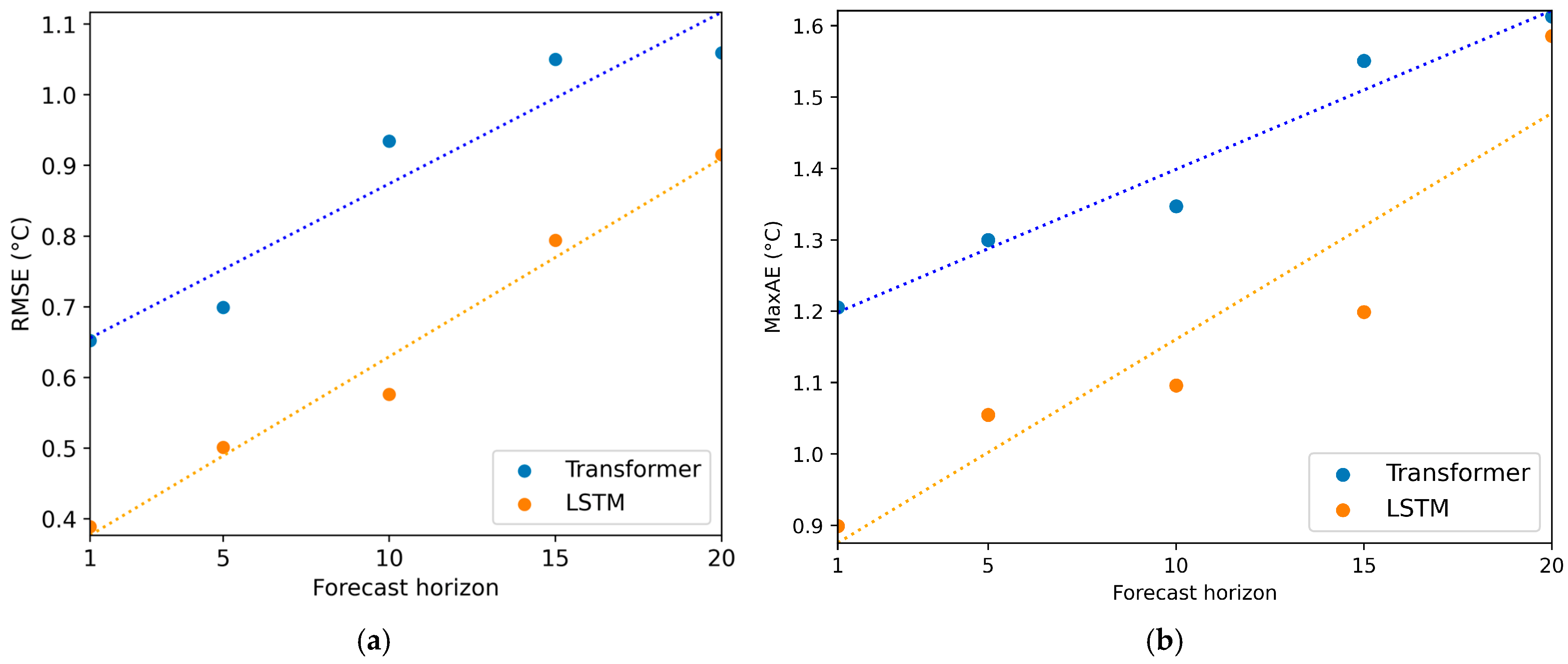
5.2. Dependence of Forecasting Errors on Forecast Horizon

To explore anticipatory capability of the ML models, predictions were calculated for forecast horizons of 1, 5, 10, 15, and 20 points using a fixed lookback window of 20 points. Figure 8a displays RMSE for Transformer (blue) and LSTM (orange) forecasting of TC1 (ETU vessel) as a function of the forecast horizon. Figure 8b displays MaxAE for Transformer (blue) and LSTM (orange) forecasting of TC1 as a function of the forecast horizon. The blue and orange dotted lines are linear regression fits. One can observe that for the range of values of the forecast horizon in Figure 8, RMSE and MaxAE of LSTM are lower than those of Transformer errors. However, the difference in errors between the respective model errors decreases with increasing forecast horizon. Moreover, the forecasting errors of LSTM increased more rapidly with increasing forecast horizons, as compared to the corresponding increase in the forecasting errors of the Transformers. Using Table 2 of temperatures in the ETU vessel, the measurement uncertainty of thermocouples in ETU was max(0.75%, 2.2 °C) ≈ 3 °C. Note that the RMSE and MaxAE for all forecast horizon lengths for all thermocouples in the ETU vessel are smaller than the measurement uncertainty of 3 °C.

Table 9. R² values for linear fits of RMSE and MaxAE as functions of the forecast horizon for Transformer and LSTM predictions of temperatures of five thermocouples in the ETU vessel.

ETU Thermocouple	Transformers R2		LSTM R2
	RMSE	MaxAE	RMSE	MaxAE
TC1	0.9139	0.961	0.9797	0.8735
TC2	0.8948	0.8008	0.8191	0.9425
TC3	0.869	0.9793	0.9142	0.8981
TC4	0.874	0.9169	0.9416	0.9912
TC5	0.9612	0.9562	0.8854	0.9434

lists the R² values of the linear fits of RMSE and MaxAE dependence on the forecast horizon for the Transformer and LSTM models for five thermocouples in the ETU vessel. One can observe that both Transformer and LSTM models had R² > 0.8 for linear fits of RMSE and MaxAE dependence on the forecast horizon for all thermocouples.

The linear correlations between MaxAE and forecast horizon (fh) for TC1 through TC5 are listed in

Table 10. Linear correlations between MaxAE and forecast horizon (fh) for LSTM and Transformers. Maxfh is the value of fh for which the correlation yields MaxAE = 3 °C.

ETU Thermocouple	Transformers MaxAE		LSTM MaxAE
	Correlation	Maxfh	Correlation	Maxfh
TC1	0.0223 × fh + 1.1763	81	0.0317 × fh + 0.8437	68
TC2	0.0167 × fh + 1.6429	81	0.0357 × fh + 1.0071	55
TC3	0.0266 × fh + 1.4172	59	0.0341 × fh + 0.9345	60
TC4	0.0233 × fh + 1.6674	57	0.0359 × fh + 1.1207	52
TC5	0.0265 × fh + 0.8969	79	0.0291 × fh + 0.6986	79

. The trend for all thermocouples is that MaxAE increases with fh. The slope of the linear correlation for Transformers is in the range of 0.0167 to 0.0266. The slope of the linear correlation for LSTM is in the range 0.0291 to 0.0359. For the same thermocouples, the slope of the linear correlation for LSTM is slightly larger than the slope of the linear correlation for the Transformers. Table 10 lists the maximum forecast horizon Maxfh calculated from the linear correlations as the value of fh for which MaxAE = 3 °C (measurement uncertainty in the ETU vessel) for the LSTM and Transformer models. For both Transformers and LSTM trained with a lookback window of 20 points, the maximum forecast horizon could be at least 50 points. For the same thermocouple, Transformers allow for the same or larger forecast horizon of predictions compared to LSTM. Note that according to Table 9, R² < 0.9 for linear fits of MaxAE predictions of TC2 with Transformers, and MaxAE predictions of TC1 and TC3 with LSTM. Therefore, the estimated values of Maxfh for Transformers predictions of TC2 and for LSTM predictions of TC1 and TC3 are less accurate than other values in Table 10.

6. Conclusions

Development of robust forecasting ML models involves training them on extensive amounts of historical data. However, large amounts of training data are not available for GenIV reactor facilities, which are currently under construction. The lack of historical data can be compensated for by transfer learning (TL), which can be used to create pre-trained ML models with available data from small-scale research facilities. The pre-trained ML models can then be fine-tuned for monitoring tasks at GenIV facilities.

In this paper, we investigated the TL performance of two deep learning neural network architectures, i.e., long short-term memory (LSTM) and Transformers, for nuclear thermal hydraulics monitoring tasks. We developed pre-trained LSTM and Transformer forecasting models by training on augmented temperature measurements from thermal hydraulic research flow loops with water and Galinstan fluids at room temperature. The pre-trained Transformer and LSTM models were then fine-tuned and re-trained with minimal additional data to perform forecasting of time series data from high temperature measurements at the ETU facility at Kairos Power. Re-training was performed using a relatively small fraction of the initial low temperature augmented data, scaled to the average temperature of the ETU facility and a minimal amount (<1%) of ETU data from correlated thermocouples. Both LSTM and Transformer models performed predictions with a forecast horizon of 10 points, for lookback window sizes equal to 1, 5, 10, 15, 20, 40, 60, 80, and 100 points. In another study, the ML models performed predictions for forecast horizons equal to 1, 5, 10, 15, and 20 points using a lookback window size of 20 points. The performance of the models was evaluated by calculating root mean squared error (RMSE) and maximum absolute error (MaxAE).

LSTM outperform Transformers for the examined range of lookback windows and forecast horizon lengths. However, LSTM errors increase more rapidly with increasing lookback window size and increasing forecast horizon lengths as compared to the pattern for the Transformers errors. For a fixed forecast horizon size of 10 points, the optimal lookback window sizes are in the vicinity of 20 points for both models. For a fixed lookback window size of 20 points, Transformers and LSTM allow for a forecast horizon of at least 50 points before the error in predictions becomes comparable with uncertainty in measurements.

Future work will extend this analysis to forecast temperature time series in high temperature liquid sodium and molten salt facilities. We will also investigate forecasting of the time series of other sensor measurements, such as flow and pressure. In addition, we will consider the performance of different deep learning architectures, including classifiers such as Extreme Gradient Boost (XGBoost), in transfer learning tasks.

References

1. Locatelli, G.; Mancini, M.; Todeschini, N. Generation IV nuclear reactors: Current status and future prospects. Energy Policy 2013, 61, 1503–1520. [Google Scholar] [CrossRef]
2. Forsberg, C. The advanced high-temperature reactor: High-temperature fuel, liquid salt coolant, liquid-metal-reactor plant. Prog. Nucl. Energy 2005, 47, 32–43. [Google Scholar] [CrossRef]
3. Ayo-Imoru, R.M.; Cilliers, A.C. A survey of the state of condition-based maintenance (CBM) in the nuclear power industry. Ann. Nucl. Energy 2018, 112, 177–188. [Google Scholar] [CrossRef]
4. Ayo-Imoru, R.M.; Cilliers, A.C. Continuous machine learning for abnormality identification to aid condition-based maintenance in nuclear power plant. Ann. Nucl. Energy 2018, 118, 61–70. [Google Scholar] [CrossRef]
5. Rivas, A.; Delipei, G.K.; Davis, I.; Bhongale, S.; Hou, J. A system diagnostic and prognostic framework based on deep learning for advanced reactors. Prog. Nucl. Energy 2024, 170, 105114. [Google Scholar] [CrossRef]
6. Schultz, R. Role of thermal-hydraulics in nuclear power plants: Design and safety. In Thermal-Hydraulics of Water Cooled Nuclear Reactors; Woodhead Publishing: Sawston, UK, 2017; pp. 143–166. [Google Scholar]
7. Hashemian, H.; Riggsbee, E. I&C system sensors for advanced nuclear reactors. Nucl. Plant J. 2018, 36, 48–51. [Google Scholar]
8. Kumar, V.D.; Bhattacharyya, A.; Behera, R.P.; Kasinathan, M.; Prabakar, K. Degradation and residual life assessment of thermocouples with damaged sheaths in corrosive environments. J. Instrum. 2025, 20, P01002. [Google Scholar] [CrossRef]
9. Zhu, Y.; Zhao, S.; Zhang, Y.; Zhang, C.; Wu, J. A Review of Statistical-Based Fault Detection and Diagnosis with Probabilistic Models. Symmetry 2024, 16, 455. [Google Scholar] [CrossRef]
10. Mandal, S.; Santhi, B.; Vinolia, K.; Swaminathan, P. Sensor fault detection in Nuclear Power Plant using statistical methods. Nucl. Eng. Des. 2017, 324, 103–110. [Google Scholar] [CrossRef]
11. Mandal, S.; Santhi, B.; Sridhar, S.; Vinola, K.; Swaminathan, P. A novel approach for fault detection and classification of the thermocouple sensor in nuclear power plant using singular value decomposition and symbolic dynamic filter. Ann. Nucl. Energy 2021, 103, 440–453. [Google Scholar] [CrossRef]
12. Mandal, S.; Santhi, B.; Sridhar, S.; Vinolia, K.; Swaminathan, P. Minor fault detection of thermocouple sensor in nuclear power plants using time series analysis. Ann. Nucl. Energy 2019, 134, 383–389. [Google Scholar] [CrossRef]
13. Pantopoulou, S.; Weathered, M.; Lisowski, D.; Tsoukalas, L.; Heifetz, A. Temporal Forecasting of Distributed Temperature Sensing in a Thermal Hydraulic System with Machine Learning and Statistical Models. IEEE Access 2025, 13, 10252–10264. [Google Scholar] [CrossRef]
14. Lim, B.; Zohren, S. Time-series forecasting with deep learning: A survey. Philos. Trans. R. Soc. A 2021, 379, 20200209. [Google Scholar] [CrossRef] [PubMed]
15. Wapachi, F.I.; Diab, A. Time-series forecasting of a typical PWR system response under Control Element Assembly withdrawal at full power. Nucl. Eng. Des. 2023, 413, 112472. [Google Scholar] [CrossRef]
16. Pantopoulou, S.; Ankel, V.; Weathered, M.T.; Lisowski, D.D.; Cilliers, A.; Tsoukalas, L.H.; Heifetz, A. Monitoring of Temperature Measurements for Different Flow Regimes in Water and Galinstan with Long Short-Term Memory Networks and Transfer Learning of Sensors. Computation 2022, 10, 108. [Google Scholar] [CrossRef]
17. Fu, Y.; Zhang, D.; Xiao, Y.; Wang, Z.; Zhou, H. An Interpretable Time Series Data Prediction Framework for Severe Accidents in Nuclear Power Plants. Entropy 2023, 25, 1160. [Google Scholar] [CrossRef]
18. Mandal, S.; Santhi, B.; Sridhar, S.; Vinola, K.; Swaminathan, P. Nuclear power plant thermocouple sensor-fault detection and classification using deep learning and generalized likelihood ratio test. IEEE Trans. Nucl. Sci. 2017, 64, 1526–1534. [Google Scholar] [CrossRef]
19. Wang, W.; Yu, J.; Xu, T.; Zhao, C.; Zhou, X. On-line abnormal detection of nuclear power plant sensors based on Kullback-Leibler divergence and ConvLSTM. Nucl. Eng. Des. 2024, 428, 113489. [Google Scholar] [CrossRef]
20. Dong, F.; Chen, S.; Demachi, K.; Yoshikawa, M.; Seki, A.; Takaya, S. Attention-based time series analysis for data-driven anomaly detection in nuclear power plants. Nucl. Eng. Des. 2023, 404, 112161. [Google Scholar] [CrossRef]
21. Yi, S.; Zheng, S.; Yang, S.; Zhou, G.; Cai, J. Anomaly Detection for Asynchronous Multivariate Time Series of Nuclear Power Plants Using a Temporal-Spatial Transformer. Sensors 2024, 24, 2845. [Google Scholar] [CrossRef]
22. Zhou, G.; Zheng, S.; Yang, S.; Yi, S. A Novel Transformer-Based Anomaly Detection Model for the Reactor Coolant Pump in Nuclear Power Plants. Sci. Technol. Nucl. Install. 2024, 2024, 9455897. [Google Scholar] [CrossRef]
23. Li, C.; Li, M.; Qiu, Z. A long-term dependable and reliable method for reactor accident prognosis using temporal fusion transformer. Front. Nucl. Eng. 2024, 3, 1339457. [Google Scholar] [CrossRef]
24. Shi, J.; Wang, S.; Qu, P. Time series prediction model using LSTM-Transformer neural network for mine water inflow. Sci. Rep. 2024, 14, 18284. [Google Scholar] [CrossRef]
25. Noyunsan, C.; Katanyukul, T.; Saikaew, K. Performance evaluation of supervised learning algorithms with various training data sizes and missing attributes. Eng. Appl. Sci. Res. 2018, 45, 221–229. [Google Scholar]
26. Zhuang, F.; Qi, Z.; Duan, K.; Xi, D.; Zhu, Y.; Zhu, H.; Xiong, H.; He, Q. A comprehensive survey on transfer learning. Proc. IEEE 2020, 109, 43–76. [Google Scholar] [CrossRef]
27. Weiss, K.; Khoshgoftaar, T.M.; Wang, D. A survey of transfer learning. J. Big Data 2016, 3, 9. [Google Scholar] [CrossRef]
28. Cinar, E. A Sensor Fusion Method Using Transfer Learning Models for Equipment Condition Monitoring. Sensors 2022, 22, 6791. [Google Scholar] [CrossRef]
29. Li, J.; Lin, M.; Li, Y.; Wang, X. Transfer learning with limited labeled data for fault diagnosis in nuclear power plants. Nucl. Eng. Des. 2022, 390, 111690. [Google Scholar] [CrossRef]
30. Tanaka, N.; Moriya, S.; Ushijima, S.; Koga, T.; Eguchi, Y. Prediction method for thermal stratification in a reactor vessel. Nucl. Eng. Des. 1990, 120, 395–402. [Google Scholar] [CrossRef]
31. Lin, T.; Wang, Y.; Liu, X.; Qiu, X. A survey of transformers. AI Open 2022, 3, 111–132. [Google Scholar] [CrossRef]
32. Vaswani, A. Attention is all you need. In Advances in Neural Information Processing Systems; The MIT Press: Cambridge, MA, USA, 2017. [Google Scholar]
33. Cabral, A.; Bakhtiari, S.; Elmer, T.W.; Heifetz, A.; Lisowski, D.D.; Carasik, L.B. Measurement of flow in a mixing Tee using ultrasound Doppler velocimetry for opaque fluids. Trans. Am. Nucl. Soc. 2019, 121, 1643–1645. [Google Scholar]
34. Blandford, E.; Brumback, K.; Fick, L.; Gerardi, C.; Haugh, B.; Hillstrom, E.; Zweibaum, N. Kairos power thermal hydraulics research and development. Nucl. Eng. Des. 2020, 364, 110636. [Google Scholar] [CrossRef]
35. Greenacre, M.; Groenen, P.J.; Hastie, T.; d’Enza, A.I.; Markos, A.; Tuzhilina, E. Principal component analysis. Nat. Rev. Methods Primers 2022, 2, 100. [Google Scholar] [CrossRef]
36. Oh, C.; Han, S.; Jeong, J. Time-series data augmentation based on interpolation. Procedia Comput. Sci. 2020, 175, 64–71. [Google Scholar] [CrossRef]
37. Koparanov, K.A.; Georgiev, K.K.; Shterev, V.A. Lookback Period, Epochs and Hidden States Effect on Time Series Prediction Using a LSTM based Neural Network. In Proceedings of the 28th National Conference with International Participation “Telecom 2020”, Sofia, Bulgaria, 29–30 October 2020. [Google Scholar]
38. Kahraman, A.; Hou, P.; Yang, G.; Yang, Z. Comparison of the Effect of Regularization Techniques and Lookback Window Length on Deep Learning Models in Short Term Load Forecasting. In Proceedings of the 2021 International Top-Level Forum on Engineering Science and Technology Development Strategy, Nanjing, China, 14–22 August 2021; Lecture Notes in Electrical Engineering. Springer: Singapore, 2022; Volume 816. [Google Scholar]
Figure 1. Schematic diagram of Transformer network architecture.
Energies 18 02286 g001
Figure 2. Positions of thermocouples W1 to W7 in water-filled flow loop. An identical configuration was set up for the Galinstan-filled flow loop to obtain measurements with thermocouples G1 through G7.
Energies 18 02286 g002
Figure 3. (a) Positions of selected thermocouples TC1 to TC5 in the ETU vessel. (b) Time series of selected thermocouples TC1 though TC5 in the ETU vessel.
Energies 18 02286 g003
Figure 4. Importances of thermocouples in the top zone (Z1) of the vessel.
Energies 18 02286 g004
Figure 5. Importances of thermocouples of water (W1–W7) and Galinstan (G1–G7) flow loops, using three principal components.
Energies 18 02286 g005
Figure 6. Heatmap of Euclidean distances between ETU vessel thermocouple pairs.
Energies 18 02286 g006
Figure 7. Forecasting errors of TC1 with Transformers (blue) and LSTM (orange) models with different lookback window sizes. (a) RMSE and (b) MaxAE. Fitting curves are 4th order polynomials.
Energies 18 02286 g007
Figure 8. Errors in forecasting of TC1 with Transformer (blue) and LSTM (orange) models as functions of the forecast horizon. (a) RMSE and (b) MaxAE.
Energies 18 02286 g008