A Multistage Physics-Informed Neural Network for Fault Detection in Regulating Valves of Nuclear Power Plants

Abstract

In Nuclear Power Plants (NPPs), online condition monitoring and the fault detection of structures, systems and components (SSCs) can aid in guaranteeing safe operation. The use of data-driven methods for these tasks is limited by the requirement of physically consistent outcomes, particularly in safety-critical systems. Considering the importance of regulating valves (e.g., safety relief valves and main steam isolation valves), this work proposes a multistage Physics-Informed Neural Network (PINN) for fault detection in such components. Two stages of the PINN are built by developing the process model of the regulating valve, which integrates the basic valve sizing equation into the loss function to jointly train the two stages of the PINN. In the 1st stage, a shallow Neural Network (NN) with only one hidden layer is developed to estimate the equivalent flow coefficient (a key performance indicator of regulating valves) using the displacement of the valve as input. In the 2nd stage, a Deep Neural Network (DNN) is developed to estimate the flow rate expected in normal conditions using inputs such as the estimated flow coefficient from the 1st stage, the differential pressure, and the fluid temperature. Then, the residual, i.e., the difference between the estimated and measured flow rates, is fed into a Deep Support Vector Data Description (DeepSVDD) to detect the occurrence of faults. Moreover, the deviation between the estimated flow coefficients of normal and faulty conditions is used to interpret the consistency of the detection result with physics. The proposed method is, first, applied to a simulation case implemented to emulate the operating characteristics of regulating the valves of NPPs and then validated on a real-world case study based on the DAMADICS benchmark. Compared to state-of-the-art fault detection methods, the obtained results from the proposed method show effective fault detection performance and reasonable flow coefficient estimation, thus guaranteeing the physical consistency of the detection results.

1. Introduction

In general, a Nuclear Power Plant (NPP) consists of structures, systems and components (SSCs), some of which are critical for safety and operational thermal efficiency of the NPP [1]. Operational interruptions of these SSCs can result in a million-dollar loss a day [2]. Therefore, accurate online condition monitoring and anomaly detection are necessary and crucial for these SSCs of a NPP [3]. One of the important SSCs is the regulating valve, which is widely used in different parts of the NPP for various purposes to ensure the safe and reliable operation of the whole system [4]. Such valves include safety/relief valves used in the pressurizer for regulating the pressure of the nuclear reactor coolant inventory, main steam isolation valves used in the main steam system for the rapid and tight closure of primary containment isolation, and turbine regulating/control valves used in the turbine system for regulating the steam flow to the turbine [5]. It is highly desirable to detect faults in regulating valves as early as possible before they become inoperable.

Over the past decades, a wide range of methods for Fault Detection and Diagnosis (FDD) has been proposed within NPP applications, thus ranging from model-based and signal processing-based approaches to artificial intelligence-based and machine learning-based techniques. In [6], a model-based method using a subspace identification model was developed to detect faulty sensors. In [7], a signal-processing method based on time–frequency analysis was proposed, thus focusing on vibration signals to identify the operational status of various components in NPPs. In [8], a novel method based on the transformation of impact signals using the Wigner–Ville distribution was proposed to estimate the location of loose parts. In [9], a Long Short-Term Memory (LSTM) network was developed to perform sensor fault detection using labeled simulation data. In [10], a convolutional gated recurrent network aided by particle swarm optimization for hyperparameters tuning was proposed to perform fault diagnosis using a simulation dataset. A detailed review of the methods developed for FDD in NPPs can be found in [2].

Despite these developments, there are few reported works on the detection of faults in regulating valves. In [11], a method was proposed for the fault-critical point prediction of a gate valve based on the characteristic analysis of the operational process variables using experimental data. In [12], a fault prediction method combining Principal Component Analysis (PCA) and a neural network using experimental data was developed. In [13], a gate recurrent unit-based method was developed for the fault diagnosis of electric gate valves using features extracted from vibration signals. In [14], a fault diagnosis method for electric isolation valves was developed by combining a knowledge-based rule reasoning model and a data-driven gate recurrent unit model.

The fault detection and diagnostic of regulating valves in other industries are also receiving attention. In [15], a model-based method for fault detection and isolation was proposed using fuzzy modeling to derive nonlinear models for the processes under normal and faulty conditions. The residuals obtained from these models were then used for fault detection. In [16], an online fault detection method was proposed for monitoring the signal values of the valve supply current and spool position in relation to the spool positioning control signal. In [17], a fault detection method was proposed based on canonical variate analysis using the simulation data of a benchmark model for a pneumatic control valve used in the power, food processing, and chemical industries. In [18], a method based on Support Vector Machines (SVMs) was developed for fault detection in a pneumatic control valve used in the manufacturing industry. In [19], a fault diagnostic and prognostic method based on SVMs and an Adaptive Neurofuzzy Inference System (ANFIS) was developed for a hydrocontrol valve used in the aerospace industry.

On the other hand, with the recent advancements in artificial intelligence, deep learning-based approaches have attracted attention in the field of Prognostics and Health Management (PHM), thanks to their powerful automatic feature extraction and nonlinear fitting capabilities [20,21]. In [22], a valve stiction detection method based on the Convolutional Neural Network (CNN) was developed. In [23], an internal leakage detection method based on the CNN was developed using the power spectral density images of acoustic emission signals. While these methods have performed well with large amounts of data, pure data-driven deep learning approaches generally violate physics-based laws with a lack of explainability of the detection and diagnostic results due to their black box nature. Hence, with the Physics-Informed Neural Network (PINN), a new variant of the Neural Network (NN) has been proposed in recent research works to make the black box model physically meaningful, interpretable, and applicable to different industrial scenarios by incorporating physical constraints from domain knowledge.

The demand for model interpretability and physical consistency in the PHM field has led to the recognition of the PINN as a highly promising method to improve the performance and interpretability of maintenance decision making [24]. In [25], a physics-informed deep learning approach based on the CNN was developed using a physics-driven loss function derived from physical knowledge to improve fault detection accuracy. In [26], a PINN method based on Autoencoders (AEs) was developed by integrating the physics law of the current–voltage relation into the loss function to perform high impedance fault detection. In [27], a physics-guided CNN was developed in which the CNN kernel was designed using the physical knowledge of the faulty signal of rolling element bearings. With respect to industrial actuators, only a few approaches of the PINN have been reported in the literature. In [28], the PINN was used for system identification in servohydraulic shaking tables. In [29], the PINN was used for the prediction of displacement in soft pneumatic actuators. In [30], the PINN was used for distinguishing anomalies caused by the faults of actuators and sensors. Notice that these applications of the PINN are for specific objectives other than for fault detection in regulating valves.

In this context, a multistage PINN combined with a Deep Support Vector Data Description (SVDD) for fault detection in regulating valves is proposed in this work. Two stages of the PINN model are built by developing the process model of the regulating valves to estimate the flow rate expected under normal conditions. In the 1st stage, a shallow NN with only one hidden layer is used to estimate the equivalent flow coefficient (a key performance indicator of the regulating valve) using the displacement of the valve as input. In the 2nd stage, a Deep Neural Network (DNN) with multiple hidden layers is used to estimate the flow rate, thus using as inputs the estimated flow coefficient from the 1st stage, the differential pressure of the regulating valve, and the liquid temperature. The development of the two stages for the PINN instead of a single deep PINN is motivated by the relevance of the flow coefficient, which serves as an input to the 2nd stage. The physics-informed loss function must also take into account this parameter (see Section 3.1.2), given its relevance in determining the flow capacity of the regulating valves [31]. Thus, by implementing the two stages of the PINN, the model can well capture the underlying physical relationships and dependencies within the system. To jointly and effectively train the multistage PINN, the basic valve sizing equation is incorporated into the PINN using a novel physical loss function. In this way, the PINN model can estimate the flow coefficient without the need for real labels. Note that the addition of the physical loss function is the primary difference between the PINN and conventional NN, which allows for training the PINN so as to conform as much as possible to the relevant physical principles under consideration. Finally, the residual of the estimation, i.e., the difference between the estimated and the measurement of flow rate, is fed into the DeepSVDD [32], which is a deep learning variant of the SVDD that uses a DNN as a mapping function instead of a kernel function to detect the anomaly in regulating valves. In the DeepSVDD, the classifier learns to recognize the boundaries or characteristics of a single class based on the training data containing samples of only that class. The objective is to obtain a classifier that enables recognition of that class, thereby allowing the detection of all other samples not from the class as anomalies or outliers. This approach is commonly used in scenarios where samples from other classes are rare, unknown, or unavailable during the training process. In the present work, a strategy is also developed for online updating of the 1st stage of the multistage PINN for the estimation of the online flow coefficient.

The proposed method is applied to a simulation case study and then validated on a real-world case study based on the “Development and Application of Methods for Actuator Diagnosis in Industrial Control Systems” (DAMADICS) benchmark [31]. The obtained results, in comparison to other state-of-the-art methods, demonstrate the effectiveness of the proposed method for fault detection in regulating valves.

The main contributions of this work are as follows:

(1)

The development of a multistage PINN model for the estimation of the flow rate signal of regulating valves;

(2)

The formulation of a physically consistent loss function for training the multistage PINN to estimate the flow coefficient based on the online updating strategy in the absence of real labeled input data;

(3)

The use of DeepSVDD to analyze residuals for fault detection, without the need to manually set the threshold.

The remainder of the paper is organized as follows. Section 2 formulates the problem. In Section 3, the proposed method is presented, and the metrics used to assess its performance are outlined in Section 4. The application of the proposed method to both simulation and real-world case studies is discussed in Section 5. Finally, Section 6 presents the conclusions of the work.

2. Problem Statement

We consider a control/regulating valve, which is one of the important components of an NPP in which multiple degradation modes can occur. The valve is typically monitored by measuring a set of N physical quantities at a generic time, t, which can be formalized into the vector:

$$\begin{array}{c}\hfill \overrightarrow{x}\left(t\right)=[x_{t,1},\cdots ,x_{t,j},\cdots ,x_{t,N}]\end{array}$$

(1)

Such quantities include the fluid temperature, the displacement of the valve, and the differential pressure, which are expected to contain information correlated to the flow rate, $Q\left(t\right)$, of the regulating valve, which is a crucial sensory measurement at time, t.

Without loss of generality, the dataset $D^{train}={[\overrightarrow{x}\left(t\right),Q\left(t\right)]}_{t=1,\dots ,T}$ collected over a period of time during normal operating conditions of the regulating valve is assumed to be available, which contains the following:

(1)

The measurement $\mathbf{X}\in {\mathbb{R}}^{T\times N}$, which is historically collected during the past operation of the regulating valve, which is an $\mathit{N}$-dimensional variable signal matrix, with $x_{t,j}$, $t=1,\dots T$, $j=1,\dots N$ being the measurement of the physical quantity j at time t;

(2)

The flow rate measurement $\mathbf{Q}\in {\mathbb{R}}^T$ collected during the past operation of the regulating valve, which is a vector, with $Q\left(t\right)$, $t=1,\dots T$ being the measurement of the flow rate at time t.

Based on the above assumption, and considering a new test input ${\overrightarrow{x}}_{test}\left(t\right)$ and its corresponding flow rate $Q_{test}\left(t\right)$ measured at current time t, the objective of the present work is to develop a data-driven dynamic process model, $f\left(·\right)$, that represents the behavior of regulating valves in normal condition, for which we have the following:

(1)

It receives in input the online measurement ${\overrightarrow{x}}_{test}\left(t\right)$ at the current time t and produces in output the estimate ${\widehat{Q}}_{test}\left(t\right)$ of the observation $Q_{test}\left(t\right)$ expected in the normal condition;

(2)

It detects the occurrence of a fault using the analysis of the residual, ${\widehat{Q}}_{test}\left(t\right)-Q_{test}\left(t\right)$, between the estimate ${\widehat{Q}}_{test}\left(t\right)$ and the observation $Q_{test}\left(t\right)$ at the current time t.

3. Proposed Method

The proposed method for the detection of faults in regulating valves is sketched in Figure 1. It consists of a multistage PINN for the estimation of the flow coefficient and flow rate (Section 3.1), as well as a DeepSVDD for the analysis of residuals for fault detection (Section 3.2). The implementation procedure of the proposed method for fault detection is described in Section 3.3.

3.1. Multistage PINN Model

3.1.1. Basic Valve Sizing Equation

Regulating valves aim to prevent, allow, and properly limit the flow of fluids through the systems to ensure reliable operation. Generally, the correct sizing of a regulating valve is crucial to maintain a desired set point. Based on fluid mechanics theory, a basic control/regulating valve sizing equation can be derived [33]:

$$\begin{array}{c}\hfill Q=C_v\sqrt{\frac{\Delta p}{\rho }}\end{array}$$

(2)

$$\begin{array}{c}\hfill c_v=\frac{C_v}{\sqrt{\rho }}\end{array}$$

(3)

where Q is the flow rate; $C_v$ is the liquid sizing coefficient indicating the flow capacity of the valve; $\Delta p$ is the differential pressure across the valve; and $\rho$ is the liquid specific gravity. $c_v$ is defined here as the equivalent to $C_v$ (equivalent flow coefficient, a key performance indicator of regulating valves), as the value of $\rho$ is unknown and always assumed to be constant during operation [34]. This equation is used for formulating the physical loss function for the multistage PINN training. The motivation of using the PINN to estimate $c_v$ is that the values of the flow coefficient (liquid sizing coefficient) are unknown in this work, so the flow rate cannot be computed even if the equation is in a closed form. In some cases, flow coefficients can be obtained from some manufacturing specifications, but the coefficient gradually changes over the period of operation as the valve ages, which makes it difficult to obtain the accurate coefficient values during operation.

3.1.2. Definition of the Multistage PINN Loss Function

The proposed multistage PINN aims to estimate the flow rate signal at time t using the input signals, $\overrightarrow{x}\left(t\right)=[\Delta p\left(t\right),dis\left(t\right),tem\left(t\right)]$, where $dis\left(t\right)$ is the displacement of the regulating valve, and $tem\left(t\right)$ is the fluid temperature. To estimate $c_v$ without using real labels, the two-stage PINN is designed such that the 1st stage is modeled with a shallow NN, $f_{{\theta }_A}$, which enables efficient online updating, and the 2nd stage is modeled with a DNN, $f_{{\theta }_D}$, which is a deeper network used to capture the complex relationships in the data for estimating the flow rate signal (Figure 1):

$$\begin{array}{c}\hfill \widehat{c}\left(t\right)=f_{{\theta }_A}\left(dis\left(t\right)\right)\end{array}$$

(4)

$$\begin{array}{c}\hfill \widehat{Q}\left(t\right)=f_{{\theta }_D}(\Delta p\left(t\right),\widehat{c}\left(t\right),tem\left(t\right))\end{array}$$

(5)

where ${\theta }_A$ and ${\theta }_D$ are the vectors of the shallow NN and DNN parameters, respectively. The set of trainable parameters $[{\theta }_A,{\theta }_D]$ are optimized jointly during the supervised training phase, whose objective is to minimize the estimation error of $\widehat{Q}$ via a physically consistent loss function:

$$\begin{array}{c}\hfill \underset{{\theta }_A,{\theta }_D}{argmin}{L}_{total}\end{array}$$

(6)

with

$$\begin{array}{c}\hfill L_{total}=(1-\mu )L_{data}+\mu L_{phy}\end{array}$$

(7)

where $L_{data}$ is the data-driven loss function, $L_{phy}$ is the physical loss function, and $\mu$ is the hyperparameter that indicates the importance given to $L_{phy}$ with respect to $L_{data}$ during model training. The data-driven loss function is formulated using the mean squared error:

$$\begin{array}{c}\hfill L_{data}=\frac{1}{T}\sum _{t=1}^T{(\widehat{Q}\left(t\right)-Q\left(t\right))}^2\end{array}$$

(8)

where $Q\left(t\right)$ is the actual value of the flow rate, and T is the number of patterns in $D^{train}$. Conversely, the physical loss function is derived from the derivative of Q with respect to $c_v$:

$$\begin{array}{c}\hfill \frac{dQ}{d{c}_v}=\sqrt{\Delta p}\end{array}$$

(9)

$$\begin{array}{c}\hfill L_{phy}=\frac{1}{T}\sum _{t=1}^T(\frac{d\widehat{Q}\left(t\right)}{d{\widehat{c}}_v\left(t\right)}-\sqrt{\Delta p\left(t\right)})\end{array}$$

(10)

The formulation of the physical loss function is designed such that its reliance on the actual labels of $C_v$ can be eliminated, which is an achievable task through the utilization of the Automatic Differentiation feature inherent in Neural Networks [35]. Consequently, the estimation of $\widehat{c}\left(t\right)$ is rendered independent of the necessity for real labels, thereby establishing it as a viable surrogate for the Health Indicator (HI). This, in turn, facilitates the interpretation of fault detection results.

The hyperparameter $\mu$ in Equation (7) can be optimized based on the model performance on the validation set. In this work, a two-step process is adopted for determining the hyperparameter $\mu$ by optimization. First, the value of $\mu$ is set to 0 to determine the optimal model architecture; then, a grid search approach is applied, where the value of $\mu$ is varied between 0 and 1 to obtain the best physically consistent trained model.

3.2. Analysis of Residuals by DeepSVDD for Fault Detection

Following the development of the multistage PINN model for predicting Q, an unsupervised method based on DeepSVDD is developed to analyze the residuals for detecting the occurrence of a fault. DeepSVDD is used instead of deterministic threshold approaches, which require the proper setting of the threshold. This is an application-specific complex task that can result in either large false alarm rates if the threshold is too small or large missed alarm rates if the threshold is too large. SVDD is a technique related to the One Class-SVM (OC-SVM) that uses a kernel-based method for mapping the data into a high-dimensional feature space to find the smallest hypersphere, instead of a hyperplane, with center m and radius $R>0$ that enclose the majority of the data in normal conditions. DeepSVDD is an extension of SVDD that uses deep learning, like DNNs, to learn effective representations of the data with an SVDD objective. DeepSVDD does not rely on predefined kernel functions, thus allowing for more effective feature extraction and making it suitable for complex and large datasets.

Assume that a validation dataset $D^{val}={[\overrightarrow{x}\left(k\right),Q\left(k\right)]}_{k=1,\dots ,N}$ collected during normal operating conditions is also available, which can be arranged into sequences of n matrices, with each having a time window length of w with $ss$ sliding steps and $(w-ss)$ overlapping between two consecutive time windows. The anomaly indicator ($AI$) for the ith time window is defined as follows:

$$\begin{array}{c}\hfill A{I}_i={∥{\overrightarrow{r}}_i∥}_{L_2}^2;i=1,2,\dots ,n\end{array}$$

(11)

where ${\overrightarrow{r}}_i={\overrightarrow{\widehat{Q}}}_i-{\overrightarrow{Q}}_i$ is the residual of the ith time window predicted by $\left\{f_{{\theta }_A},f_{{\theta }_D}\right\}$. The anomaly indicators $A{I}^{val}$, computed from $D^{val}$, are mapped onto $n_{sd}$ feature representations using a DNN, $f_{{\theta }_{sd}}$, of the DeepSVDD. The aim of $f_{{\theta }_{sd}}$ is to define a more compact space where $A{I}^{val}$ falls within, whereas the $AI$ from abnormal conditions does not. The boundary of the discovered compact space is the hypersphere of the minimal volume characterized by center m and radius R of the minimal volume (Figure 2). The center m of the hypersphere can be calculated as the mean of the $f_{{\theta }_{sd}}$ representations that result from the $f_{{\theta }_{sd}}$ initialization during the first forward iteration of the procedure. The training of the DeepSVDD is achieved through the optimization of the following objective function:

$$\begin{array}{c}\hfill argmin\frac{1}{n}\sum _{i=1}^n{∥f_{{\theta }_{sd}}\left(A{I}_i\right)-m∥}^2+\frac{\lambda }{2}\sum _{l=1}^L{∥{\theta }_{sd}^l∥}_F^2\end{array}$$

(12)

where $f_{{\theta }_{sd}}$ is the DNN of the DeepSVDD contains L hidden layers, and ${\theta }_{sd}=\left\{{\theta }_{sd}^1,\cdots ,{\theta }_{sd}^L\right\}$ are the parameters of each layer. Specifically, $f_{{\theta }_{sd}}\left(A{I}_i\right)$ is the learned representation of the input $A{I}_i$ from the network $f_{{\theta }_{sd}}$ with parameters ${\theta }_{sd}$. The primary goal of the DeepSVDD is to learn ${\theta }_{sd}$ by identifying a hypersphere of the minimum volume with center m. Minimizing ${∥f_{{\theta }_{sd}}\left(A{I}_i\right)-m∥}^2$ minimizes the volume of the hypersphere. The second term in the objective function represents a weight decay regularizer with a hyperparameter $\lambda >0$, where ${∥·∥}_F^2$ denotes the Frobenius norm. To bring the data as close to the center m as possible, the DNN must extract the common factors of variation. Once trained, the radius R is defined as the 90th percentile of ${∥f_{{\theta }_{sd}}\left(A{I}_i\right)-m∥}_{i=1,\dots ,n}$ calculated across all training instances. During testing, the DeepSVDD model determines the outcome by comparing R with the distance calculated between m and $f_{{\theta }_{sd}}\left(A{I}_{test}\right)$ (i.e., ${∥f_{{\theta }_{sd}}\left(A{I}_{test}\right)-m∥}_{i=1,\dots ,n}$), where a fault is identified if the latter exceeds R.

3.3. Implementation Procedure of the Proposed Method

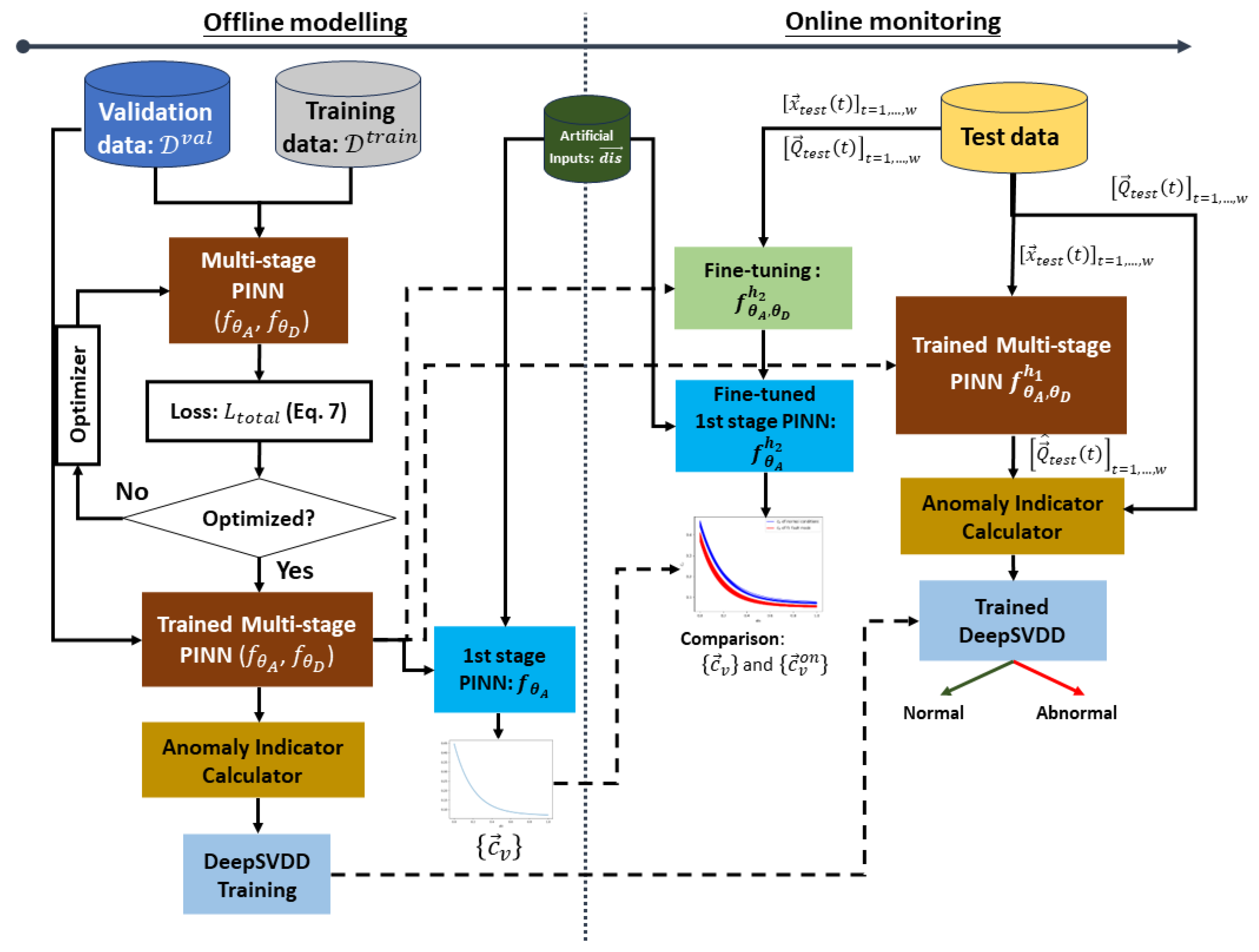
The implementation procedure of the proposed method described above is depicted in Figure 3, thus comprising two parts: offline modeling and online monitoring.

3.3.1. Offline Modelling

The offline modeling utilizes historical normal operating data, divided into training set $D^{train}={[\overrightarrow{x}\left(t\right),Q\left(t\right)]}_{t=1,\dots ,T}$ and validation set $D^{val}={[\overrightarrow{x}\left(k\right),Q\left(k\right)]}_{k=1,\dots ,K}$. In the offline modeling, the training of the proposed method consists of two phases: the training of the multistage PINN and the training of the DeepSVDD.

The multistage PINN is, first, trained by minimizing the multistage loss function (Equation (7)). The hyperparameter, $\mu$ in Equation (7), is set using a grid search approach on the validation set.

To train the DeepSVDD, the following sequential steps are first implemented:

(1)

Rearrange the validation set into $n=(K-w)/ss$ matrices, with each having a time window length w with $(w-ss)$ overlapping between consecutive time windows, as described in Section 3.2. This results in sequences of an array of n matrices, ${\mathbf{A}}^{val}\in {\mathbb{R}}^{n\times w\times (N+1)}$, with $A_i^{val}={[\overrightarrow{x}\left(l\right),Q\left(l\right)]}_{l=1:w}$ being the matrix of the ith time window, $i=1,2,\dots ,n$, in the array;

(2)

Predict the flow rates for each ith time window in ${\mathbf{A}}^{val}$ using the trained multi stage PINN, $\left\{f_{{\theta }_A},f_{{\theta }_D}\right\}$;

(3)

Compute the corresponding anomaly indicator $A{I}_i$ for the predicted flow rates in step (2) using Equation (11), thus resulting in $A{I}^{val}={\left[A{I}_i\right]}_{i=1,\dots ,n}$.

Then, the DeepSVDD is trained using the data $A{I}^{val}$ by optimizing Equation (12) to obtain a decision function $f_{sd}\left(A{I}^{val}\right)$.

Finally, a baseline for the equivalent flow coefficient curve, ${\overrightarrow{c}}_v$, indicates the normal operating condition of a regulating valve and is established through the following sequential steps:

(1)

The incremental displacement input, ${\overrightarrow{dis}}^c={\left[di{s}_i^c\right]}_{i=1,\dots ,N_d}$, is artificially generated:

$$\begin{array}{c}\hfill di{s}_i^c=\frac{i}{N^d},i=1,\dots ,N_d\end{array}$$

(13)

This represents the operational process of regulating valves from fully open to closed, as described in [31]. $N_d$ is set to 100 in this work;

(2)

The generated ${\overrightarrow{dis}}^c$ is used as input to the 1st stage of the trained multistage PINN, $f_{{\theta }_A}$, to estimate ${\overrightarrow{c}}_v$, which is a health indicator reflecting the flow capacity at different opening statuses of the regulating valve.

A plot of ${\overrightarrow{c}}_v$ against the artificially generated displacement, ${\overrightarrow{dis}}^c$, establishes a baseline for the equivalent flow coefficient curve of the regulating valve operating under normal conditions.

3.3.2. Online Monitoring

The online monitoring of the proposed method requires w successive online observations, $X_{test}\left(t\right)={\left[{\overrightarrow{x}}_{test}\left(t\right)\right]}_{t=1,\dots ,w}$, to reconstruct the measurements $Q_{test}\left(t\right)={\left[{\overrightarrow{Q}}_{test}\left(t\right)\right]}_{t=1,\dots ,w}$ expected in normal conditions. After w successive online observations, for any subsequent $ss$ consecutive online observations, the matrix $X_{test}$ and the corresponding vector $Q_{test}\left(t\right)$ are retroactively updated from the current measurement backward to the size of the moving time window w. The updated $X_{test}$ is then used for predictions. The online monitoring comprises two parts:

(1)

The estimation of the flow rates, ${\widehat{Q}}_{test}\left(t\right)$, expected in normal conditions for fault detection;

(2)

The estimation of the online equivalent flow coefficient, ${\overrightarrow{c}}_v^{on}$, which is a health indicator used for interpreting the consistency of the detection outcomes with physics.

With respect to (1), the trained multistage PINN $\left\{f_{{\theta }_A},f_{{\theta }_D}\right\}$ in Section 3.3.1 is stored as $f_{{\theta }_A,{\theta }_D}^{h1}$ and is utilized to predict the ${\widehat{Q}}_{test}$ expected in normal conditions. The predictions are used by the anomaly indicator calculator, thus providing input $A{I}_{test}$ to the trained DeepSVDD, which outputs the prediction $f_{{\theta }_{sd}}\left(A{I}_{test}\right)$. The regulating valve condition is then considered "normal" if ${∥f_{{\theta }_{sd}}\left(A{I}_{test}\right)-m∥}^2\le R$ and “abnormal” otherwise.

With respect to (2), the trained multistage PINN $\left\{f_{{\theta }_A},f_{{\theta }_D}\right\}$ in Section 3.3.1 is separately stored as $f_{{\theta }_A,{\theta }_D}^{h2}$, which is fine-tuned online using $X_{test}$. Fine-tuning involves updating only the 1st stage of the PINN, $f_{{\theta }_A}^{h_2}$, by freezing the parameters ${\theta }_D$ of the 2nd stage $f_{{\theta }_D}^{h_2}$ and updating the parameters ${\theta }_A$ of $f_{{\theta }_A}^{h_2}$ through the optimization of the multistage loss function (Equation (7)). Subsequently, the equivalent flow coefficient curve, ${\overrightarrow{c}}_v^{on}$, is established by the updated model $f_{{\theta }_A}^{h2}$ using ${\overrightarrow{dis}}^c$ as input. The difference between the baseline ${\overrightarrow{c}}_v$ and the online estimation ${\overrightarrow{c}}_v^{on}$ can reflect potential degradation modes by analyzing flow capacity variation, and this can be used to interpret the physical consistency of the fault detection results.

In this work, the response time of the proposed fault detection method depends on the size, w, of the time window that is used to compute the anomaly indicators: it has been set to 100 s with a delay of 10 s (sliding step, ss). After the initialization of the model for online application, w is updatedevery 10 s. If a faulty transient process is shorter than the $ss$, the fault cannot be detected instantly.

4. Performance Metrics

The performance evaluation of the proposed method for fault detection employs various metrics, including accuracy, precision, recall, F1-score, and the Area Under the receiver operating characteristic Curve ($AUC$) [36]. Specifically, the correct classification of abnormal condition patterns is referred to as the true positive ($tp$), whereas the correct classification of normal condition patterns is referred to as the true negative ($tn$). The false positive ($fp$) represents the misclassification of normal condition patterns as abnormal, and the false negative ($fn$) represents the misclassification of abnormal condition patterns as normal.

The $Accuracy$ is defined as the fraction of correctly classified patterns among all patterns:

$$\begin{array}{c}\hfill Accuracy=\frac{tp+tn}{tp+tn+fp+fn}\end{array}$$

(14)

The $Accuracy$ is used to evaluate the overall classification performance on both normal and abnormal patterns. It is effective when there is no significant class imbalance.

The $Precision$ is defined as the fraction of abnormal condition patterns correctly classified among those patterns identified as abnormal:

$$\begin{array}{c}\hfill Precision=\frac{tp}{tp+fp}\end{array}$$

(15)

The $Precision$ is used to evaluate the performance only on the detected abnormal condition patterns: a high $Precision$ value implies a low false alarm rate.

The $Recall$, or sensitivity, is defined as the fraction of abnormal condition patterns correctly classified among the actual abnormal condition patterns:

$$\begin{array}{c}\hfill Recall=\frac{tp}{tp+fn}\end{array}$$

(16)

The $Recall$ is used to evaluate the performance only on actual abnormal condition patterns: a high $Recall$ value implies a low missed alarm rate.

The $Specificity$ is defined as the fraction of normal condition patterns correctly classified among the actual normal condition patterns:

$$\begin{array}{c}\hfill Specificity=\frac{tn}{tn+fp}\end{array}$$

(17)

The $Specificity$ is used to evaluate the performance only on actual normal condition patterns: a high $Specificity$ value implies a low false alarm rate.

The $F1-score$ ($F_1$) is the harmonic mean of $Precision$ and $Recall$:

$$\begin{array}{c}\hfill F_1=\frac{2}{\frac{1}{Precision}+\frac{1}{Recall}}\end{array}$$

(18)

The $F1-score$ is used to evaluate the comprehensive performance considering the false and missed alarm rate. It provides a single value that captures the trade-off between $Precision$ and $Recall$, thus making it particularly useful when dealing with uneven class distributions.

The $Receiver$ $Operating$ $Characteristic$ $\left(ROC\right)$ $curve$ is a curve generated by plotting the recall against the false positive rate ($FPR$):

$$\begin{array}{c}\hfill FPR=\frac{fp}{fp+tn}\end{array}$$

(19)

The $Area$ $Under$ $the$ $ROC$ $Curve$ ($AUC$) is calculated using an average of trapezoidal approximations. It particularly shows the performance on distinguishing normal and abnormal conditions. The values of the performance metrics $Accuracy$, $Precision$, $Recall$, $F1-score$, and $AUC$, range between 0 and 1, with a larger value indicating better performance.

5. Applications

Considering the unavailability of real data collected from regulating valves in NPPs, two case studies based on the DAMADICS benchmark [31] have been considered: (1) a synthetic case study designed to emulate the real industrial application of a control/regulating valve (Section 5.1) and (2) a real case study concerning the time series data collected from the operational activities of regulating valves installed in actual industrial plants (Section 5.2).

5.1. Synthetic Case Study

5.1.1. Benchmark Description

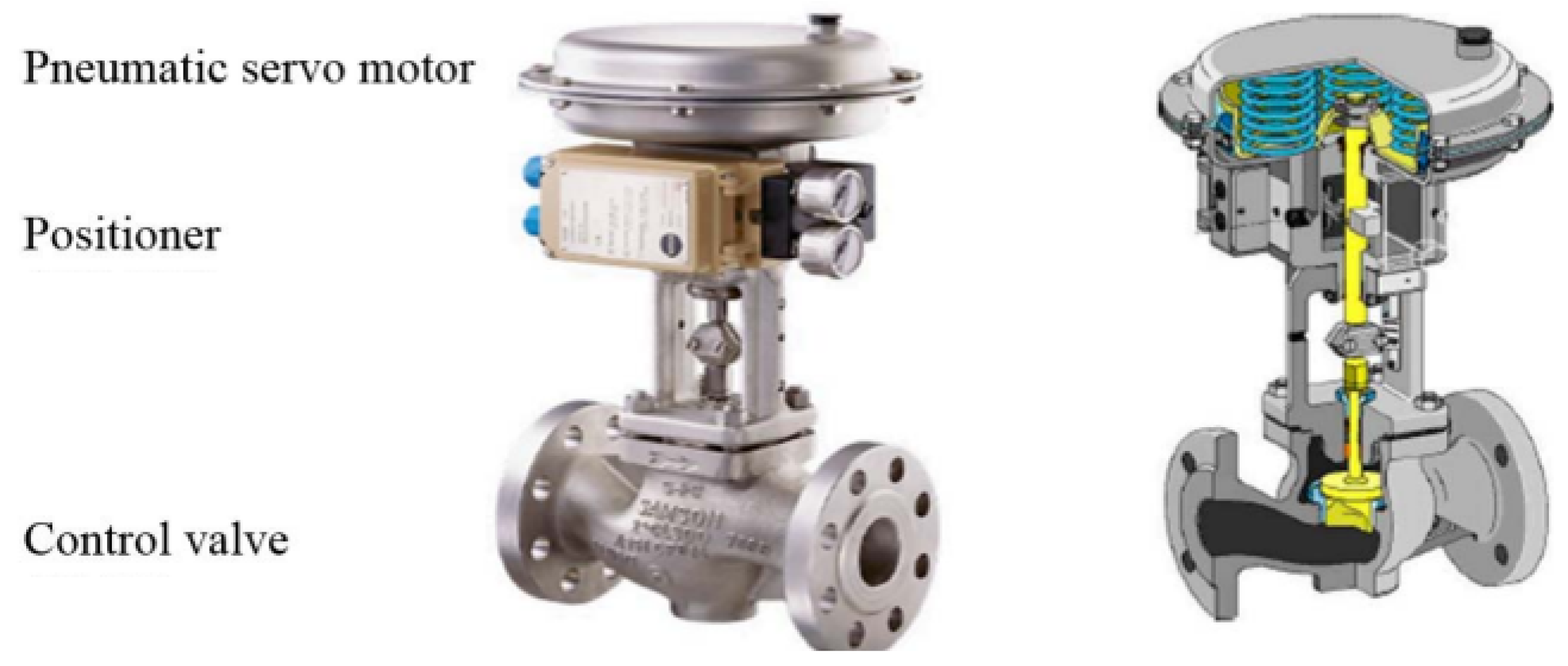
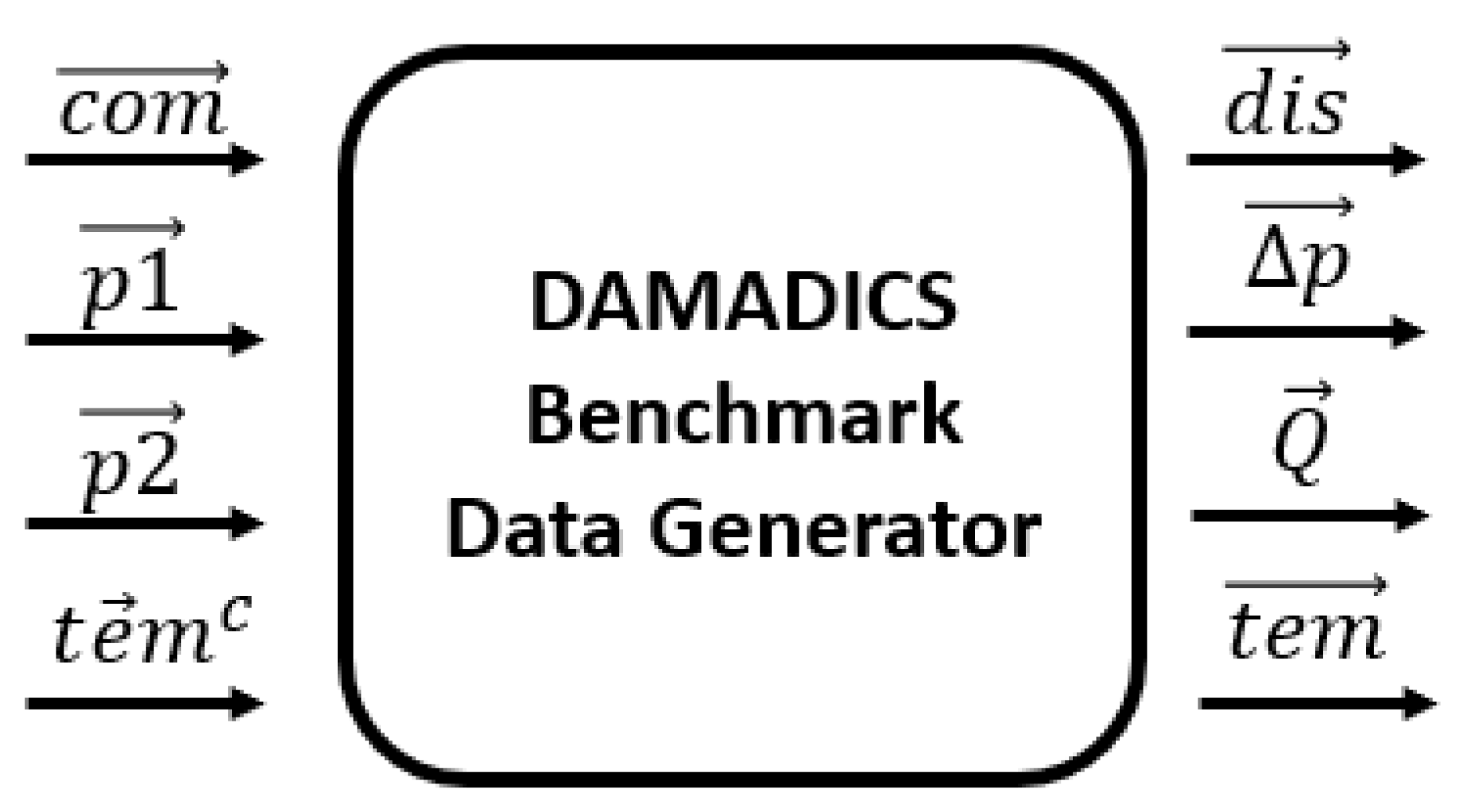
The model of an industrial control valve within the DAMADICS benchmark [31] is adopted to simulate operational data. This type of control/regulating valve is commonly used in various industrial systems, including NPPs, and therefore, it is employed in this work to simulate the operational scenarios of regulating valves, thus addressing the real data scarcity issue prevalent in NPPs. The structure of the control valve considered is depicted in Figure 4. During its operation, an electrical signal from the external controller is converted into a pressure signal via a diaphragm. The positioner ensures the generation of the correct pressure, following which a pneumatic servo motor adjusts the valve plug to the desired position for controlling/regulating the flow rate. The DAMADICS benchmark model, denoted as $f_m\left(·\right)$, is shown in Figure 5. The input signals to the model are the command signal, $\overrightarrow{com}$, which is provided by the user or the operational schedule to maintain the optimal functioning of the industrial component; the upstream and downstream fluid pressures $\overrightarrow{p1}$ and $\overrightarrow{p2}$, which represent the uncertainties in working conditions; and the fluid temperature ${\overrightarrow{tem}}^c$, which influences the flow principles of the fluid. The output signals, i.e., the measured signals, consist of the displacement signal $\overrightarrow{dis}$, the differential pressure of the valve $\overrightarrow{\Delta p}$, the flow rate $\overrightarrow{Q}$, and the liquid temperature $\overrightarrow{tem}$.

5.1.2. Data Generation

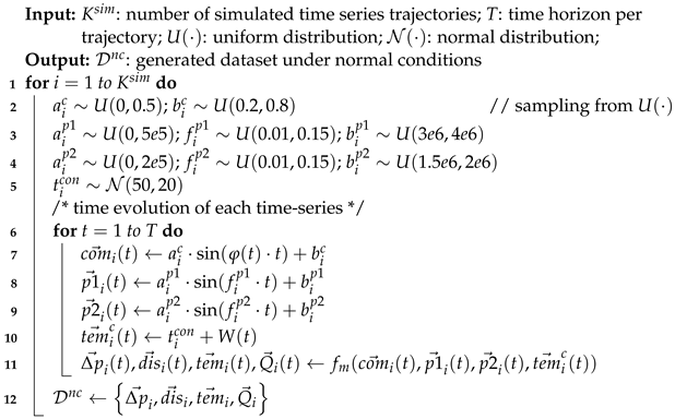
Data generation is performed using the DAMADICS model $f_m\left(·\right)$. Given the flexibility of the benchmark, the user can define appropriate simulation inputs for specific applications. To obtain the data of the variable commands and working conditions that reflect the operational activities of regulating valves in NPPs, the relevant preset inputs to $f_m\left(·\right)$ (Figure 5) have to be properly defined. In this work, they are defined as follows:

(1)

The command signal, $\overrightarrow{com}$, is defined as a chirp signal, wherein a chirp represents a signal with a varying frequency over time. By employing a chirp signal as the command signal, the dynamic behavior of the component under diverse input frequencies can be comprehensively simulated. This is motivated by the fact that the frequency response of an NPP regulating valve is an important performance indicator, which can be tested by subjecting the valve to input signals of varying frequencies [37]. The vector $\overrightarrow{com}$ is expressed as follows:

$$\begin{array}{c}\overrightarrow{com}\left(t\right)=a^c·sin\left(\phi \left(t\right)·\frac{t}{sf}\right)+b^c,\end{array}$$

(20)

$$\begin{array}{c}\phi \left(t\right)=2·\pi ·(0.1+\frac{t}{sf}).\end{array}$$

(21)

Here, $\phi \left(·\right)$ is a linear function that samples the instantaneous phase to emulate sufficiently diverse commands in realistic conditions. The parameters $a^c$ and $b^c$ are randomly sampled for each simulation from Uniform distributions, with $a^c\sim U(0,0.5)$ and $b^c\sim U(0.2,0.8)$. Additionally, $sf$ serves as the scaling factor for t, thus following $sf\sim U(200,600)$;

(2)

The upstream and downstream fluid pressures, $\overrightarrow{p1}$ and $\overrightarrow{p2}$, are defined as follows:

$$\begin{array}{c}\overrightarrow{p1}\left(t\right)=a^{p1}·sin\left(f^{p1}·t\right)+b^{p1},\end{array}$$

(22)

$$\begin{array}{c}\overrightarrow{p2}\left(t\right)=a^{p2}·sin\left(f^{p2}·t\right)+b^{p2}\end{array}$$

(23)

where $a^{p1}$, $b^{p1}$, $a^{p2}$, and $b^{p2}$ are randomly sampled from their respective Uniform distributions: $a^{p1}\sim U(0Pa,5e5Pa)$, $b^{p1}\sim U(3e6Pa,4e6Pa)$, $a^{p2}\sim U(0Pa,2e5Pa)$, and $b^{p2}\sim U(1.5e6Pa,2e6Pa)$. The pressure values are set considering the actual conditions in NPPs [38]. This ensures that the parameters are simulated within a realistic envelop of conditions. The frequencies $f^{p1}$ and $f^{p2}$ are defined frequencies of the sinusoidal signal, thus following $f^{p1}\sim U(0.01,0.15)$ and $f^{p2}\sim U(0.01,0.15)$;

(3)

The temperature of each simulation is defined as follows:

$$\begin{array}{c}{\overrightarrow{tem}}^c\left(t\right)=t^{con}+W\left(t\right)\end{array}$$

(24)

where $t^{con}$ is sampled from a Gaussian distribution $t^{con}\sim \mathcal{N}(50 °\mathrm{C},20 °\mathrm{C})$, and $W\left(t\right)$ is the white noise function accounting temperature fluctuations. The value of the temperature is set considering the real environment of the safety regulating valves, which is linked to the cooling systems in NPPs [39].

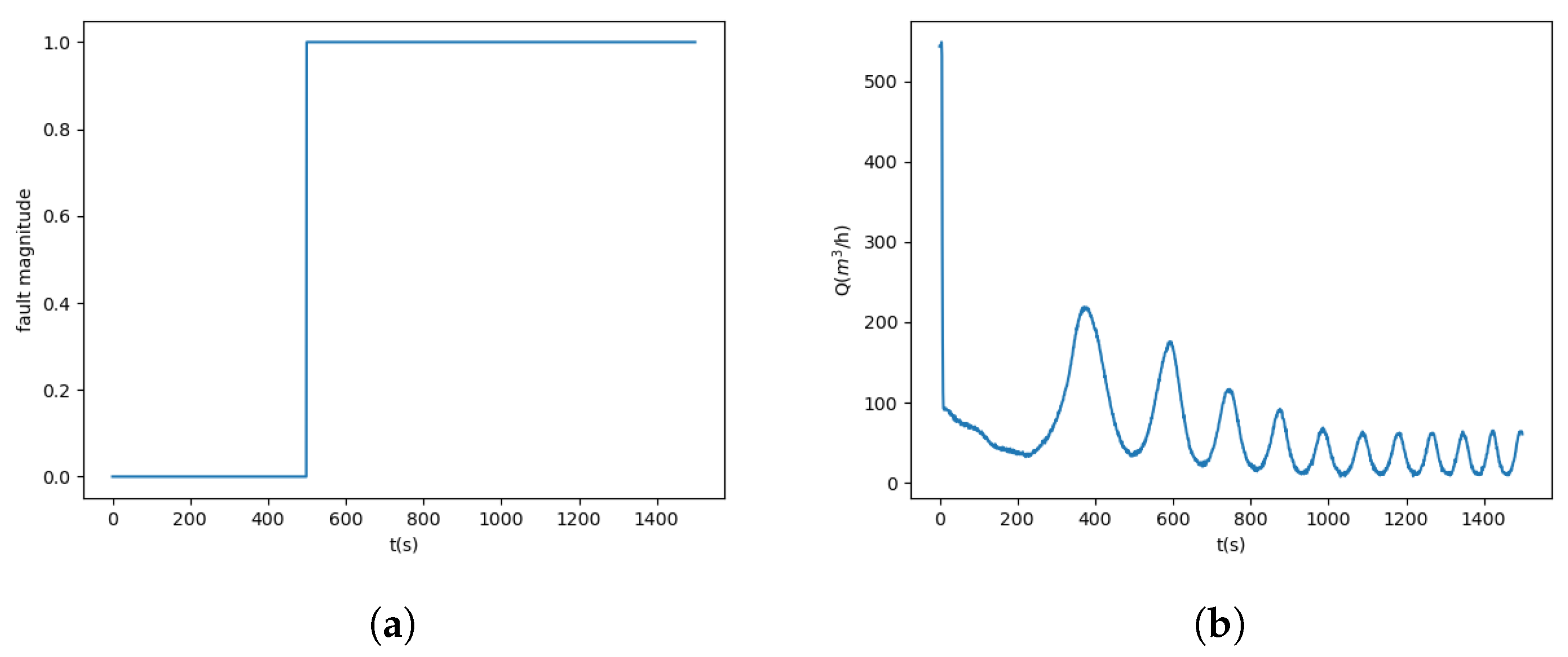
The simulation procedure for generating data is detailed in Algorithm 1 below. Subsequently, the generated normal operating condition dataset, ${\mathcal{D}}^{nc}$, containing $K^{sim}=200$ time series trajectories with each having a length of $T=500$ time series observations, is used for model development (with $D^{train}$ representing 75% of the data and $D^{val}$ representing the remaining 25%). Similarly, the test dataset, ${\mathcal{D}}^{test}$, is generated such that a fault is injected at a specific time instant in each time series (Figure 6). In this case, three fault modes, which commonly manifest in the operation of regulating valves, are considered: (1) the sedimentation of the valve plug or valve seat (denoted as “f1”); (2) the erosion of the valve plug or valve seat (denoted as “f2”); and (3) internal leakage or valve tightness (denoted as “f3”). For each fault mode, $K_f^{sim}=$30 time series trajectories are generated, with each one having a length of $T=1500$ time series observations.

Algorithm 1: Data generation using the benchmark model.

5.1.3. Results and Discussion

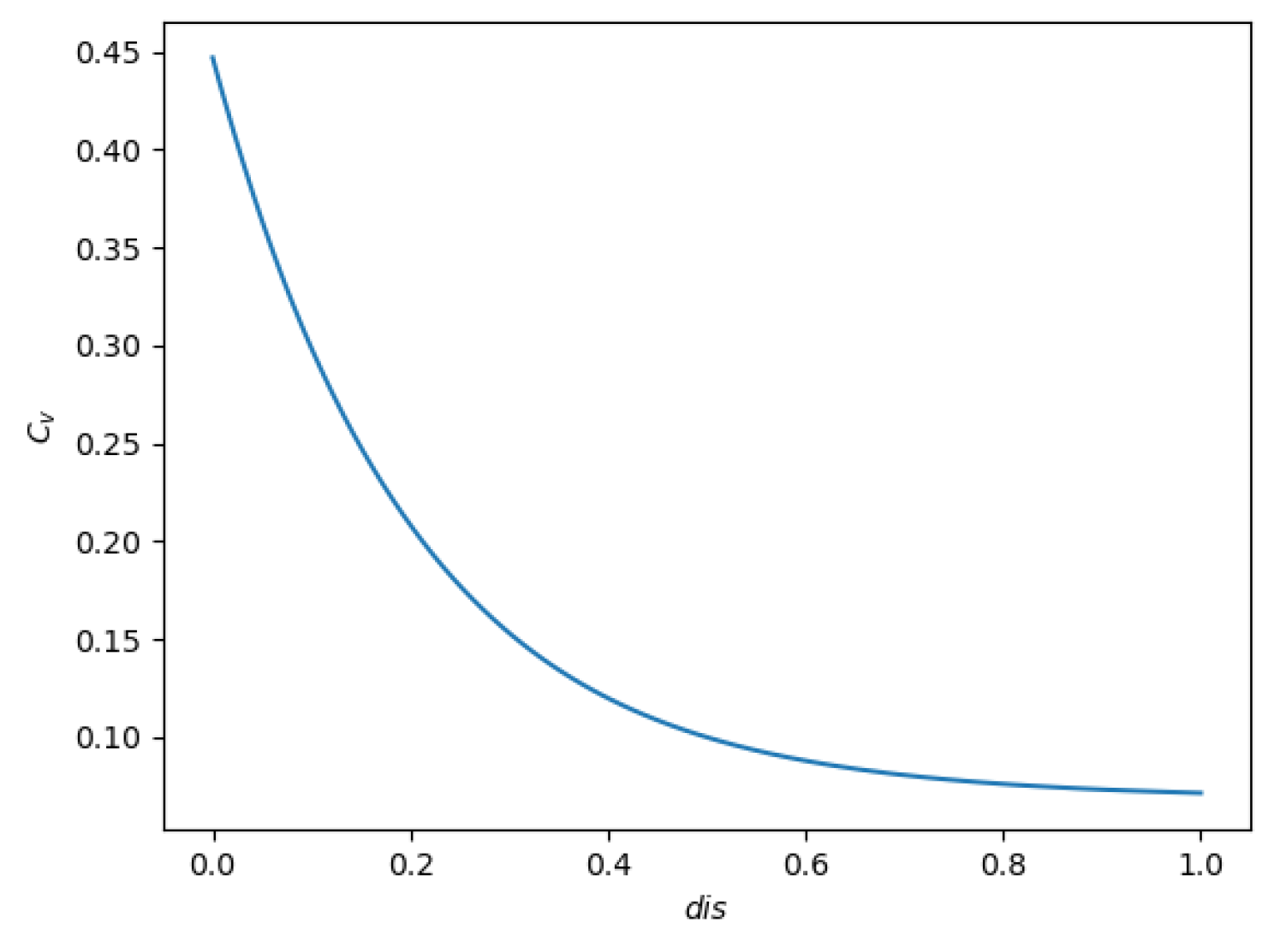
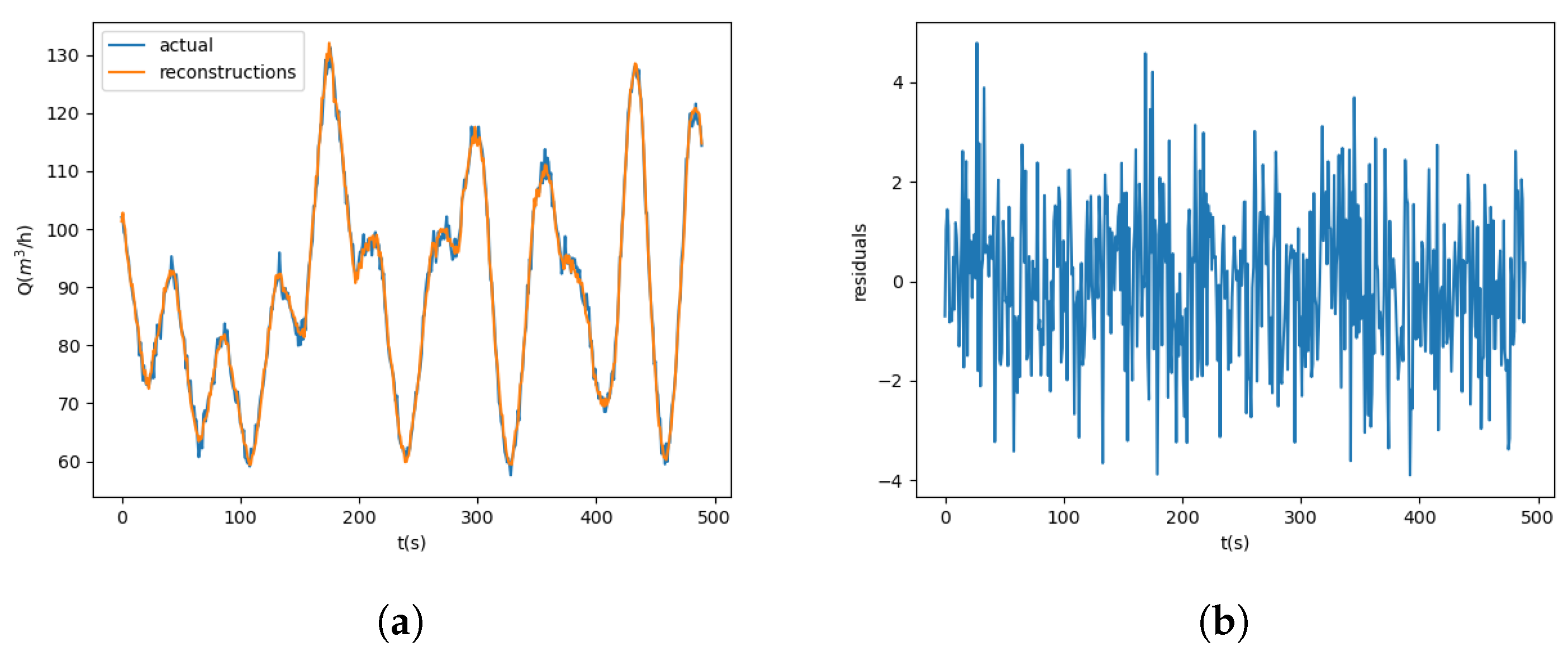
The PINN model, $\left\{f_{{\theta }_A},f_{{\theta }_D}\right\}$, was built using a shallow NN, $f_{{\theta }_A}$, with one hidden layer made by five neurons and a DNN, $f_{{\theta }_D}$, with three hidden layers made by ten neurons each. The activation function $Tanh$ was used in all layers except the output layers of $f_{{\theta }_A}$ and $f_{{\theta }_D}$ in which the $Sigmoid$ function was employed to guarantee the scale of $\overrightarrow{c}$ $\subseteq [0,1]$ [40]. To train the PINN, the Adam optimizer [41] was utilized with a learning rate $\eta =0.001$, a batch size of $L_{batch}=512$, and a number of epochs of $N_{epoch}=200$. Other architectures, e.g., a shallow NN with 10 neurons and a DNN with 20 neurons in each of the three hidden layers, have also been explored. However, these alternative architectures considered resulted in no improvement in performance while significantly increasing the computational burden of the model training. Thus, the relatively simple architecture presented in this work was preferred. The weight of the physical loss, $\mu$, was set to 0.02 through a grid search approach based on the reconstruction accuracy of the model on the validation dataset. Figure 7 shows an example of the curve that contains the estimated equivalent flow coefficient generated by the trained $f_{{\theta }_A}$ under normal conditions, which follows the expected behavior of the flow coefficient with respect to displacement [31], As shown in Figure 7, the flow coefficient decreased monotonically as the displacement increased. Although the lack of real flow coefficients made it impossible to validate the exact values in Figure 7, the obtained results follow the expected physical trend of the flow coefficient of the valve. In this work, this trend was compared with another curve that contained the estimated equivalent flow coefficients in abnormal conditions. Through this comparison, the relative difference between the two curves was used to observe the degradation in the flow capacity of the regulating valve. Figure 8 shows an example of the reconstructed flow rate signals in the validation set along with the corresponding residuals. The Root Mean Squared Error (RMSE) of the flow rate signals reconstructed by the PINN came out to 1.735.

For the DeepSVDD model, the architecture of the DNN $f_{{\theta }_{sd}}$ was composed of one hidden layer with 64 neurons and an output layer with 32 neurons ($n_{sd}=32$ feature representations), which were activated by the $Relu$ function. The batch size was set to 32, the number of epochs was set to 100, and the $Adam$ optimizer was once again employed for model training. The 32 extracted feature representations were then used to build a hypersphere that enclosed the majority of the data in normal conditions, thus enabling the detection of faults outside the hypersphere. To compute the robust anomaly indicators with the minimal false and missed alarms, the sizes of the time window w and the sliding step $ss$ were set to 100 and 10, respectively, with $w-ss$ (i.e., 100 − 10 = 90) overlapping between the two consecutive time windows.

To verify and evaluate the performance of the proposed method, the state-of-the-art fault detection methods presented in

Table 1. Comparison methods.

Method	Description	Notation
DNN	DNN model with three hidden layers and ten neurons in each layer.	$M1$
AAKR	The Auto Associative Kernel Regression (AAKR) [42] method for reconstructing all signals, $\left\{\Delta p,dis,tem,Q\right\}$. The optimal bandwidth parameter h is set to 0.15 using a grid search approach on the validation dataset, and the anomaly indicator defined in Equation (11) is used.	$M2$
AAKR	The AAKR model in $M2$ is considered, but the anomaly indicator is defined as $A{I}_i^{M3}={∥{\mathbf{R}}_i^A∥}_{L^2}^2$, where ${\mathbf{R}}_i^A$ is the residual matrix between predictions and measurements of $\left\{\Delta p,dis,tem,Q\right\}$.	$M3$
PCA	The PCA method [43] is developed to reconstruct the signals $\Delta p,dis,tem,Q$. The number of principal components selected for signal reconstruction is 3, which explains at least 80% of the data variability, and the anomaly indicator defined in Equation (11) is used.	$M4$
PCA	The PCA method in $M4$ is used, but the anomaly indicator is defined as $A{I}_i^{M5}={∥{\mathbf{R}}_i^P∥}_{L^2}^2$.	$M5$

were considered for comparison.

To ensure a fair comparison, each of the aforementioned methods for signal reconstruction was combined with DeepSVDD for fault detection.

Performance comparisons for the simulated fault modes are reported in

Table 2. Detection performance on f1: Sedimentation of valve plug or valve seat.

	M1	M2	M3	M4	M5	Proposed
Accuracy	0.9672	0.6537	0.4013	0.3132	0.3071	0.9702
Precision	0.9544	0.9203	0.7625	0.5015	0.4651	0.9585
Recall	1.0000	0.5430	0.1867	0.0619	0.0567	1.0000
Specificity	0.8951	0.8968	0.8724	0.8650	0.8569	0.9049
F1-score	0.9767	0.6830	0.2999	0.1101	0.1010	0.9788
AUC	0.9476	0.7199	0.5295	0.4635	0.4568	0.9524

,

Table 3. Detection performance on f2: Erosion of valve plug or valve seat.

	M1	M2	M3	M4	M5	Proposed
Accuracy	0.9667	0.4616	0.4191	0.3807	0.3473	0.9715
Precision	0.9537	0.8485	0.7852	0.7224	0.6386	0.9602
Recall	1.0000	0.2633	0.2126	0.1600	0.1152	1.0000
Specificity	0.8935	0.8968	0.8724	0.8650	0.8569	0.9089
F1-score	0.9763	0.4019	0.3346	0.2620	0.1952	0.9799
AUC	0.9468	0.5800	0.5425	0.5125	0.4861	0.9545

and

Table 4. Detection performance on f3: Internal leakage or valve tightness.

	M1	M2	M3	M4	M5	Proposed
Accuracy	0.9803	0.9105	0.3882	0.3285	0.3371	0.9820
Precision	0.9709	0.9763	0.6530	0.3636	0.4542	0.9732
Recall	1.0000	0.8850	0.1430	0.0320	0.0545	1.0000
Specificity	0.9429	0.9591	0.8552	0.8933	0.8752	0.9476
F1-score	0.9852	0.9284	0.2346	0.0588	0.0973	0.9864
AUC	0.9714	0.9220	0.4991	0.4627	0.4649	0.9738

. Both the proposed method and $M1$ method showed the satisfactory performance (above $0.95$) across all metrics for the three simulated fault modes of regulating valves, with the proposed method demonstrating the best performance. Although, with respect to the fault f3 (internal leakage, Table 4), the model $M2$ provided slightly larger value of $Specificity$ (a measure of how well a model is able to detect normal condition cases), and its value of Recall (a measure of how well a model is able to detect the abnormal condition cases) with respect to all of the three simulated faults was significantly smaller than that of the proposed method. Due to the strongly nonlinear relationships in the data, both the PCA and AAKR methods exhibited limitations in accurately and robustly reconstructing the signals. Consequently, these limitations led to a decrease in their fault detection performances.

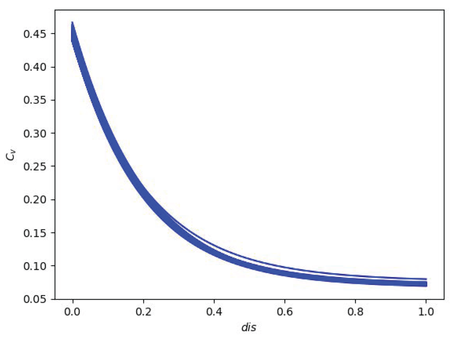
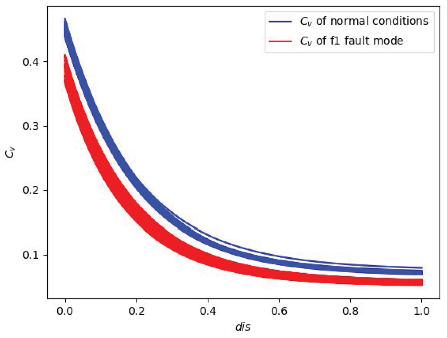
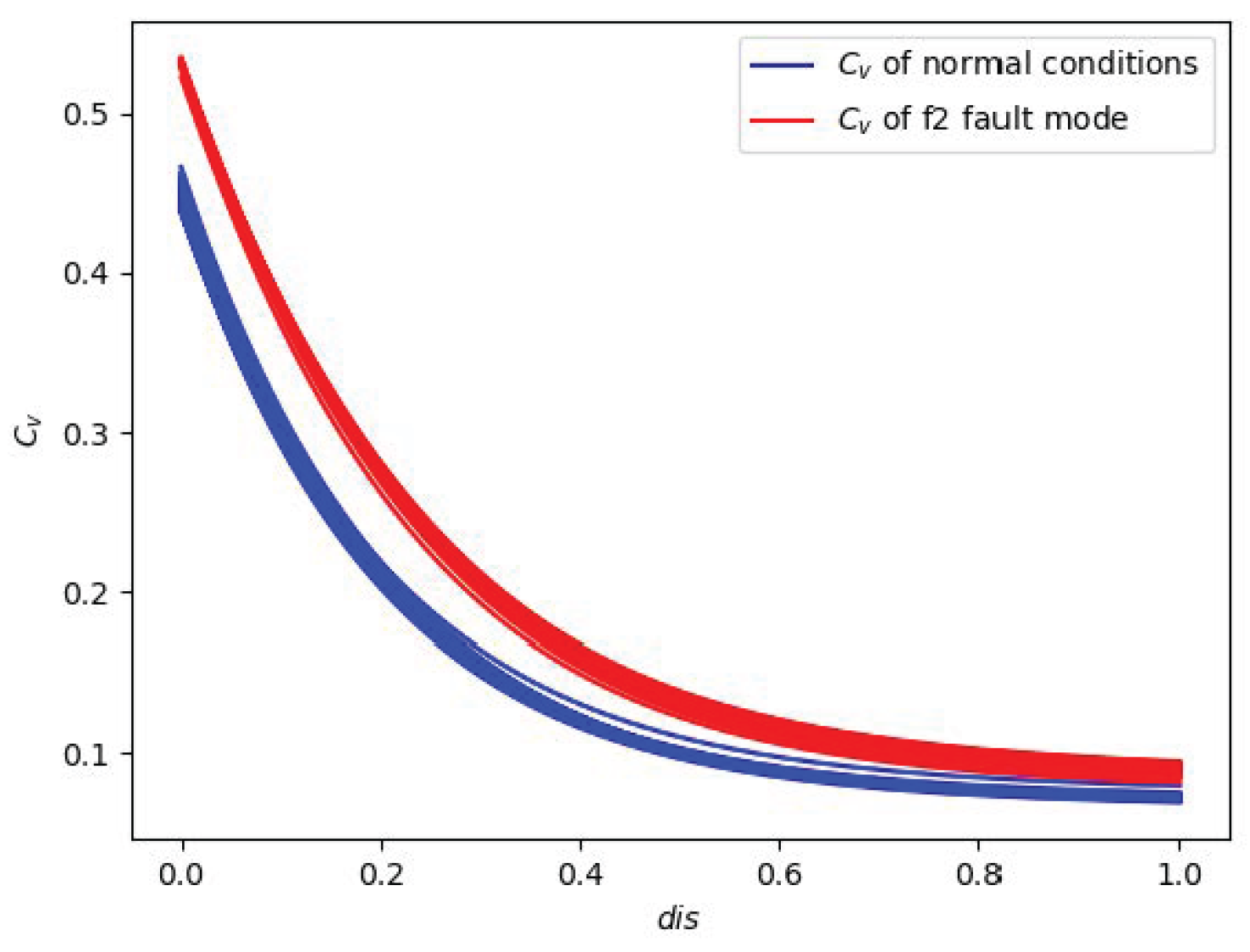
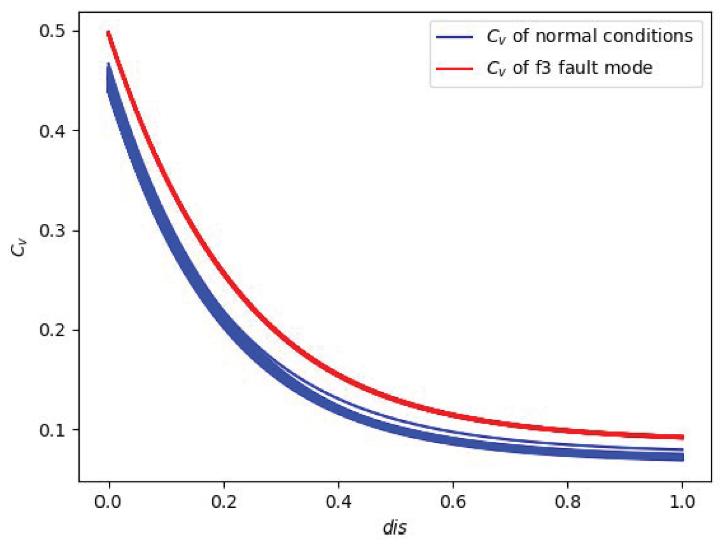
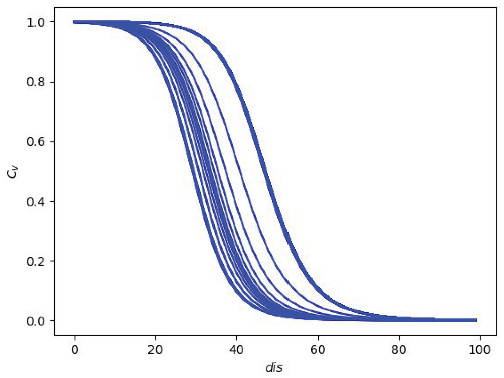
Regarding the estimated equivalent flow coefficient curves, Figure 9 shows a set of $\left\{{\overrightarrow{c}}_v\right\}$ generated from the fine-tuned models $f_{{\theta }_A}^{h2}$ using a validation dataset. $\left\{{\overrightarrow{c}}_v\right\}$ represents the healthy region of ${\overrightarrow{c}}_v$ under normal conditions, thus considering uncertainties and noise in the dataset. Figure 10 compares the $\left\{{\overrightarrow{c}}_v\right\}$ of the normal conditions and the $\left\{{\overrightarrow{c}}_v^{f1}\right\}$ of fault f1, where ${\overrightarrow{c}}_v^{f1}$ was lower at all $dis$ points, thus indicating a decrease in the flow capacity due to the occurrence of the f1 fault mode (valve seat sedimentation), which is exactly consistent with the mechanism of f1 (valve seat sedimentation can cause the possible shrinkage of the opening area, which in turn decreases the flow capacity). In contrast, Figure 11 indicates an increase in the flow capacity for the f2 fault mode (valve seat erosion), as the opening area expands in relation to the nominal area. Similarly, Figure 12 shows an increase in the flow capacity for the f3 fault mode (internal leakage). Consequently, the estimated flow coefficient curves generated by the proposed multistage PINN model follow the physics-based mechanisms of different fault modes, thus offering insights useful for maintenance engineers.

The proposed method demonstrates satisfactory fault detection performance and provides consistent interpretations for the detected faults based on the physical mechanism. This aligns with the physics-based understanding of different fault modes, thus making it useful for potentially assisting maintenance engineers in comprehending the detected faults.

5.2. Real Case Study

5.2.1. Dataset Description

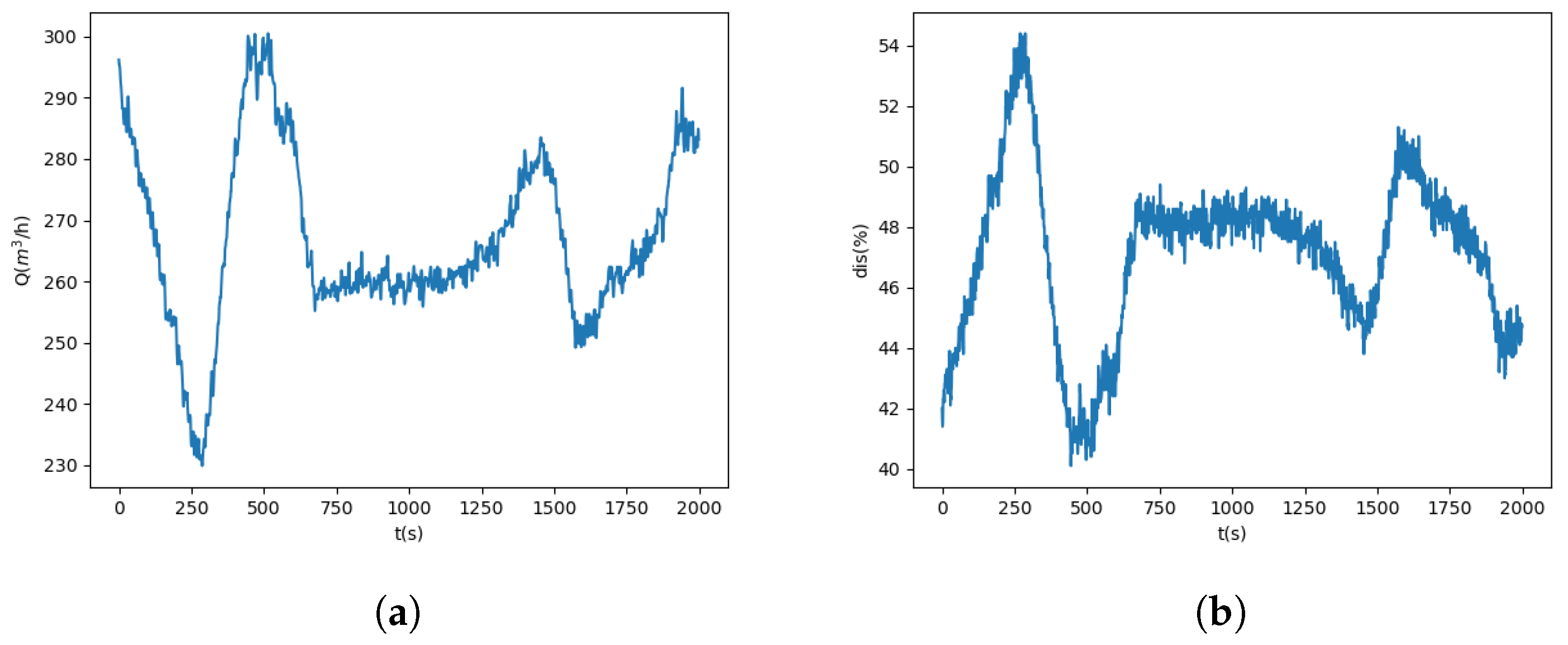
The time series data collected from a real industrial control valve within the DAMADICS benchmark project [31] were considered for the validation of the proposed method. The normal condition dataset consists of 55,000 time series observations of four signals, $\left\{\Delta p,dis,tem,Q\right\}$, which were partitioned into training and validation sets containing 45,000 and 10,000 observations, respectively. The training set was used for training the model, and the validation set was used for hyperparameter setting. Figure 13 shows the time series evolutions of Q and $dis$ under normal operating conditions. The test dataset used to assess the fault detection performance of the proposed method contains 2095 observations in the normal condition and two fault modes of 415 observations in $Partly$ $opened$ $bypass$ $fault$ (denoted as “f4”) and 205 observations in $Positioner$ $supply$ $pressure$ $drop$ (denoted as “f5”).

5.2.2. Results and Discussion

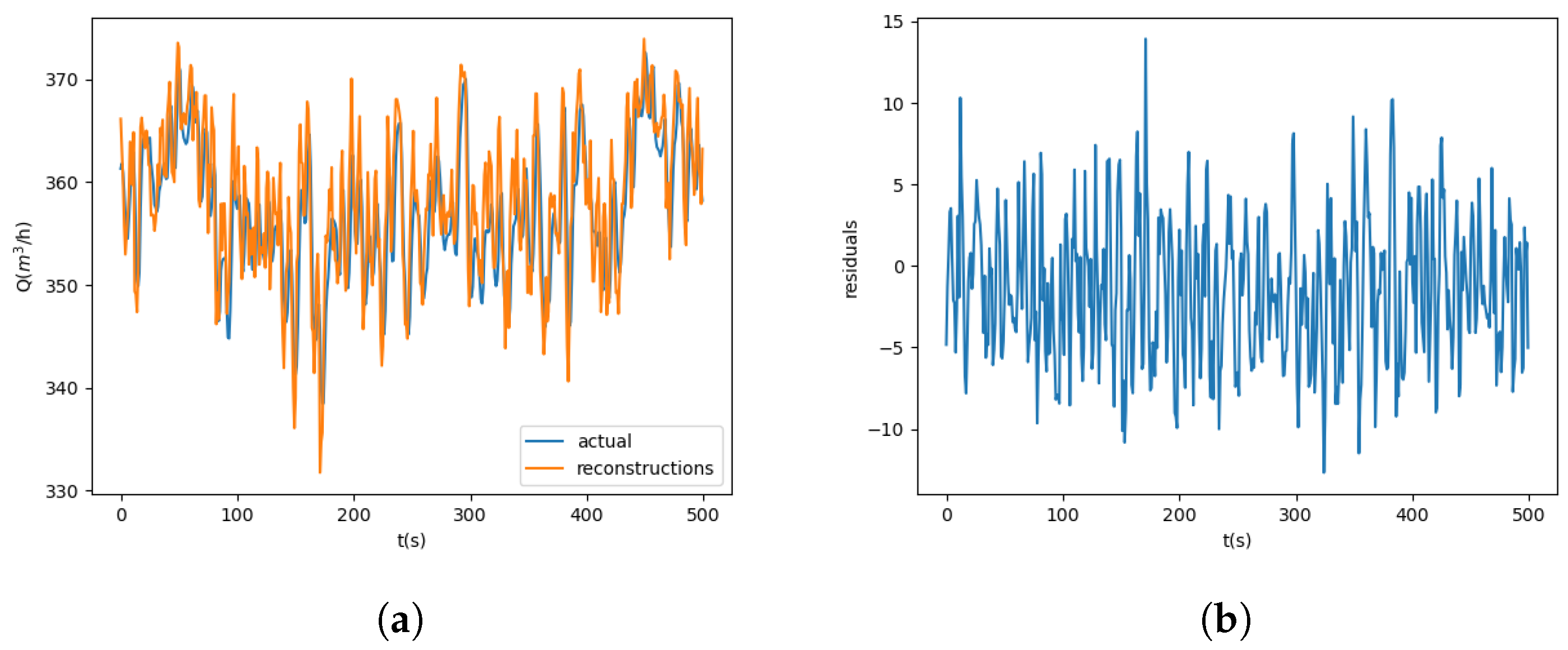
The implementation of the proposed method with respect to the real case study was similar to those of the synthetic case except that the learning rate, $\eta$, and the weight of physical loss function, $\mu$, were set to 0.003 and 0.3, respectively. Figure 14 shows an example of the reconstructed flow rate signals in the validation set along with the corresponding residuals. The RMSE of the flow rate signals reconstructed by the PINN was 4.184.

The performance of the proposed method was again compared with that of the state-of-the-art methods presented in Section 5.1.3.

Table 5. Detection performance on f4: Partly opened bypass.

	M1	M2	M3	M4	M5	Proposed
Accuracy	0.8774	0.9811	0.8774	0.7925	0.8491	0.9623
Precision	0.4583	0.8462	0.4583	0.3333	0.4074	0.8889
Recall	1.0000	1.0000	1.0000	1.0000	1.0000	0.7273
Specificity	0.8632	0.9790	0.8632	0.7684	0.8316	0.9895
F1-score	0.6286	0.9167	0.6286	0.5000	0.5790	0.8000
AUC	0.9316	0.9895	0.9316	0.8842	0.9158	0.8584

and

Table 6. Detection performance on f5: Positioner supply pressure drop.

	M1	M2	M3	M4	M5	Proposed
Accuracy	0.8594	0.8828	0.8281	0.7109	0.6797	0.9063
Precision	0.7500	0.7742	0.6136	0.4638	0.4348	0.8333
Recall	0.6563	0.7500	0.8438	1.0000	0.9375	0.7813
Specificity	0.9271	0.9271	0.8229	0.6146	0.5938	0.9479
F1-score	0.7000	0.7619	0.7105	0.6337	0.5941	0.8065
AUC	0.7917	0.8385	0.8333	0.8073	0.7656	0.8646

present the performance metrics for faults f4 and f5, respectively. With respect to fault f4 (Table 5), model $M2$ demonstrated the highest performance in terms of the accuracy, $F1-score$, and $AUC$. Model $M2$ and the proposed method showed comparable $Specificity$ values, thus indicating that both models are capable of detecting normal conditions. On the other hand, the proposed method had the highest Precision among all the models, thus suggesting its superior ability to detect abnormal conditions, which implies the lowest false alarm rate. With respect to fault f5 (Table 6), the proposed method consistently outperformed all the other models across the $Accuracy$, $Precision$, $Recall$, $Specificity$, $F1-score$, and $AUC$, which demonstrates its effectiveness in detecting both normal and abnormal conditions. It is important to note that, whereas model $M4$ achieved a perfect $Recall$ value indicating perfect performance in detecting abnormal conditions, its performance concerning other metrics was significantly lower than that of the proposed method. This also highlights the importance of considering multiple performance metrics to assess the overall effectiveness of a fault detection method. Comparing these results to the synthetic case, the performances of models $M2$, $M3$, $M4$, and $M5$ in this case study surpassed those previously obtained. This can be attributed to the relatively stable working conditions observed in the real case, as shown in Figure 13 (where the $dis$ signal varied within a limited range of 40% to 60%). In summary, the proposed method demonstrates superior overall performance for fault detection in regulating valves.

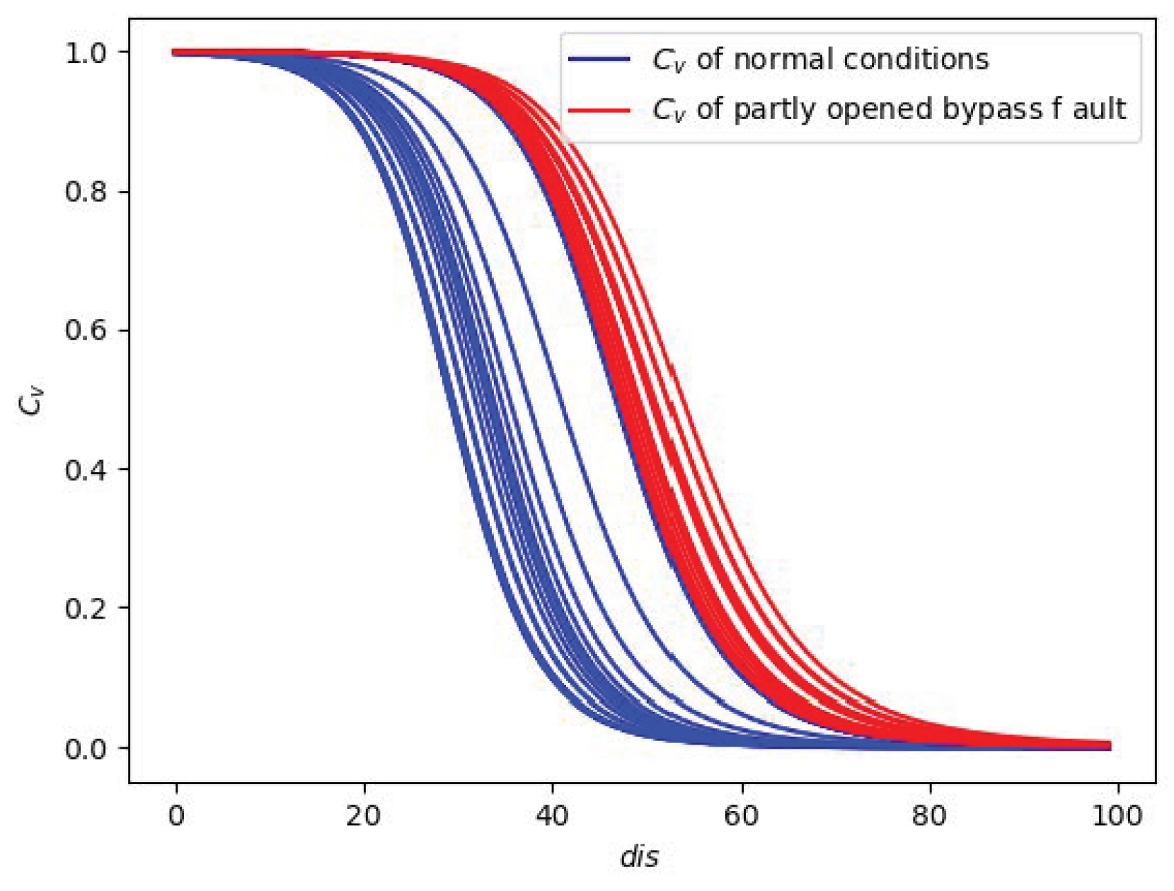
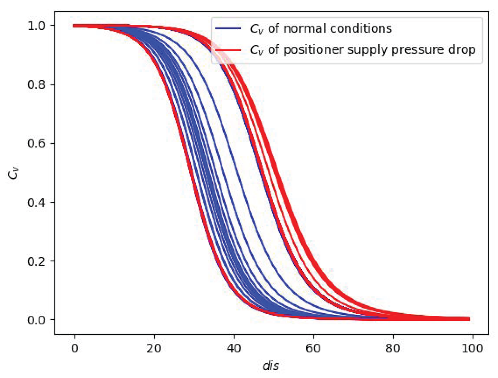
The trained proposed method was used to generate the equivalent flow coefficient curve. Figure 15 shows a set of $\left\{{\overrightarrow{c}}_v\right\}$ curves generated from the fine-tuned models $f_{{\theta }_A}^{h2}$ using the validation dataset, thus representing the healthy region of ${\overrightarrow{c}}_v$. For the $partly$ $opened$ $bypass$ fault f4, the estimated $\left\{{\overrightarrow{c}}_v^{f4}\right\}$ was significantly above $\left\{{\overrightarrow{c}}_v\right\}$ (Figure 16), thus indicating an equivalent increase in flow capacity due to the open bypass of the regulating valves. For the $positioner$ $supply$ $pressure$ $drop$ fault f5, the estimated $\left\{{\overrightarrow{c}}_v^{f5}\right\}$ was partially overlapped with $\left\{{\overrightarrow{c}}_v\right\}$ (Figure 17), thus indicating that the flow capacity of the regulating valve remained approximately equal to nominal. This observation aligns with the fault mechanism, thus indicating that the flow capacity of the regulating valve remained unaffected by the $positioner$ $supply$ $pressure$ $drop$.

In summary, the proposed method shows superior fault detection performance and provides physical insights into the detected fault modes that are consistent with the physics-based mechanisms.

6. Conclusions

In this paper, a novel method based on the multistage PINN has been developed for the detection of faults in regulating the valves of NPPs. The method consists of a muiltistage PINN proposed to estimate the flow rate signal of a regulating valve expected under normal conditions and a DeepSVDD employed to analyze the residuals (the differences between the estimates and measurements of the flow rate) for the detection of faults, thus eliminating the need for manual threshold setting. Additionally, the fundamental valve sizing equation was integrated into the multistage PINN, thus enabling the estimation of the equivalent flow coefficient curve Cv, which in turn facilitates the interpretation of the fault detection results. The proposed method was applied to two case studies from the DAMADICS benchmark: (1) a synthetic simulation case implemented to emulate the operations of regulating valves in NPPs and (2) a real dataset collected from operating industrial control valves. The obtained results show that the performance of the proposed method is more satisfactory than other state-of-the-art methods, particularly in scenarios with varying working conditions. The results also show that the deviation of the estimated $C_v$ from its nominal values can provide a rational interpretation of the occurred fault mode from the perspective of the flow capacity, which intuitively can assist maintenance engineers in subsequent maintenance decisions.

Future work will be devoted to (1) the exploration of more advanced NN techniques, such as recurrent NN, Bayesian NN, and PINNs, integrated with the physical loss function proposed in this work to enhance the model capabilities in capturing temporal dependencies and complex patterns in the data and (2) the use of real data collected from operational regulating/safety valves in NPPs to calibrate the developed model and further validate its performance.

References

1. Zio, E. Advancing nuclear safety. Front. Nucl. Eng. 2024, 2, 1346555. [Google Scholar] [CrossRef]
2. Ma, J.; Jiang, J. Applications of fault detection and diagnosis methods in nuclear power plants: A review. Prog. Nucl. Energy 2011, 53, 255–266. [Google Scholar] [CrossRef]
3. Baek, S.; Heo, G. Application of dynamic fault tree analysis to prioritize electric power systems in nuclear power plants. Energies 2021, 14, 4119. [Google Scholar] [CrossRef]
4. Lin, Z.H.; Hou, C.W.; Zhang, L.; Guan, A.Q.; Jin, Z.J.; Qian, J.Y. Fluid-structure interaction analysis on vibration characteristics of sleeve control valve. Ann. Nucl. Energy 2023, 181, 109579. [Google Scholar] [CrossRef]
5. Qian, J.Y.; Hou, C.W.; Mu, J.; Gao, Z.X.; Jin, Z.J. Valve core shapes analysis on flux through control valves in nuclear power plants. Nucl. Eng. Technol. 2020, 52, 2173–2182. [Google Scholar] [CrossRef]
6. Qin, S.; Li, W. Detection and identification of faulty sensors in dynamic processes. AIChE J. 2001, 47, 1581–1593. [Google Scholar] [CrossRef]
7. Park, G.; Lee, C.; Kim, J.; Ryu, J.; Jung, H. Identification of Nuclear Components Degradation by Time-Frequency Ridge Pattern; American Nuclear Society: La Grange Park, IL, USA, 2006. [Google Scholar]
8. Kim, Y.; Kim, S.; Chung, H.; Park, Y.; Park, J. A study on technique to estimate impact location of loose part using Wigner-Ville distribution. Prog. Nucl. Energy 2003, 43, 261–266. [Google Scholar] [CrossRef]
9. Choi, J.; Lee, S. Consistency index-based sensor fault detection system for nuclear power plant emergency situations using an LSTM network. Sensors 2020, 20, 1651. [Google Scholar] [CrossRef] [PubMed]
10. Wang, H.; Peng, M.; Ayodeji, A.; Xia, H.; Wang, x.; Li, Z. Advanced fault diagnosis method for nuclear power plant based on convolutional gated recurrent network and enhanced particle swarm optimization. Ann. Nucl. Energy 2021, 151, 107934. [Google Scholar] [CrossRef]
11. Liu, Z.; Liu, J.; Huang, Y.; Li, T.; Nie, C.; Xia, Y.; Zhan, L.; Tang, Z.; Zhang, L. Fault Critical Point Prediction Method of Nuclear Gate Valve with Small Samples Based on Characteristic Analysis of Operation. Materials 2022, 15, 757. [Google Scholar] [CrossRef]
12. An, Z.; Cheng, L.; Guo, Y.; Ren, M.; Feng, W.; Sun, B.; Ling, J.; Chen, H.; Chen, W.; Luo, Y.; et al. A Novel Principal Component Analysis-Informer Model for Fault Prediction of Nuclear Valves. Machines 2022, 10, 240. [Google Scholar] [CrossRef]
13. Huang, X.Y.; Xia, H.; Yin, W.Z.; Liu, Y.K.; Miyombo, M.E. Research on fault diagnosis method of electric gate valve under strong background noise. Ann. Nucl. Energy 2023, 194, 110055. [Google Scholar] [CrossRef]
14. Ai, X.; Yongkuo, L.; Longfei, S.; Chunli, X.; Zhou, H. A concurrent fault diagnosis method for electric isolation valves in nuclear power plants based on rule-based reasoning and data-driven methods. Prog. Nucl. Energy 2024, 170, 105190. [Google Scholar] [CrossRef]
15. Mendonça, L.F.; Sousa, J.M.C.; Costa, J.M.G. An architecture for fault detection and isolation based on fuzzy methods. Expert Syst. Appl. 2009, 36, 1092–1104. [Google Scholar] [CrossRef]
16. Raduenz, H.; Mendoza, Y.; Ferronatto, D.; Souza, F.; Bastos, P.; Soares, J.; Negri, V. Online fault detection system for proportional hydraulic valves. J. Braz. Soc. Mech. Sci. Eng. 2018, 40, 331. [Google Scholar] [CrossRef]
17. Han, X.; Jiang, J.; Xu, A.; Huang, X.; Pei, C.; Sun, Y. Fault detection of pneumatic control valves based on canonical variate analysis. IEEE Sensors J. 2021, 21, 13603–13615. [Google Scholar] [CrossRef]
18. Venkata, S.K.; Rao, S. Fault detection of a flow control valve using vibration analysis and support vector machine. Electronics 2019, 8, 1062. [Google Scholar] [CrossRef]
19. Kordestani, M.; Zanj, A.; Orchard, M.E.; Saif, M. A modular fault diagnosis and prognosis method for hydro-control valve system based on redundancy in multisensor data information. IEEE Trans. Reliab. 2018, 68, 330–341. [Google Scholar] [CrossRef]
20. Qi, B.; Liang, J.; Tong, J. Fault diagnosis techniques for nuclear power plants: A review from the artificial intelligence perspective. Energies 2023, 16, 1850. [Google Scholar] [CrossRef]
21. Yang, Z.; Baraldi, P.; Zio, E. A method for fault detection in multi-component systems based on sparse autoencoder-based deep neural networks. Reliab. Eng. Syst. Saf. 2022, 220, 108278. [Google Scholar] [CrossRef]
22. Zhang, K.; Liu, Y.; Gu, Y.; Ruan, X.; Wang, J. Multiple-timescale feature learning strategy for valve stiction detection based on convolutional neural network. IEEE/ASME Trans. Mechatronics 2021, 27, 1478–1488. [Google Scholar] [CrossRef]
23. Zhu, S.B.; Li, Z.L.; Li, X.; Xu, H.h.; Wang, X.m. Convolutional neural networks-based valve internal leakage recognition model. Measurement 2021, 178, 109395. [Google Scholar] [CrossRef]
24. Yucesan, Y.A.; Viana, F.A. A physics-informed neural network for wind turbine main bearing fatigue. Int. J. Progn. Health Manag. 2020, 11, 17. [Google Scholar] [CrossRef]
25. Shen, S.; Lu, H.; Sadoughi, M.; Hu, C.; Nemani, V.; Thelen, A.; Webster, K.; Darr, M.; Sidon, J.; Kenny, S. A physics-informed deep learning approach for bearing fault detection. Eng. Appl. Artif. Intell. 2021, 103, 104295. [Google Scholar] [CrossRef]
26. Li, W.; Deka, D. Physics-informed learning for high impedance faults detection. In Proceedings of the 2021 IEEE Madrid PowerTech, Madrid, Spain, 28 June–2 July 2021; pp. 1–6. [Google Scholar]
27. Sadoughi, M.; Hu, C. Physics-based convolutional neural network for fault diagnosis of rolling element bearings. IEEE Sensors J. 2019, 19, 4181–4192. [Google Scholar] [CrossRef]
28. Guo, W.; He, C.; Shao, P. A novel system identification method for servo-hydraulic shaking table using physics-guided long short-term memory network. Mech. Syst. Signal Process. 2022, 178, 109277. [Google Scholar] [CrossRef]
29. Sun, W.; Akashi, N.; Kuniyoshi, Y.; Nakajima, K. Physics-informed recurrent neural networks for soft pneumatic actuators. IEEE Robot. Autom. Lett. 2022, 7, 6862–6869. [Google Scholar] [CrossRef]
30. Guc, F.; Chen, Y. Fault Cause Assignment with Physics Informed Transfer Learning. IFAC-PapersOnLine 2021, 54, 53–58. [Google Scholar] [CrossRef]
31. Bartyś, M.; Patton, R.; Syfert, M.; de las Heras, S.; Quevedo, J. Introduction to the DAMADICS actuator FDI benchmark study. Control Eng. Pract. 2006, 14, 577–596. [Google Scholar] [CrossRef]
32. Yi, J.; Yoon, S. Patch svdd: Patch-level svdd for anomaly detection and segmentation. In Proceedings of the Asian Conference on Computer Vision 2020, Kyoto, Japan, 30 November–4 December 2020. [Google Scholar]
33. Bartyś, M. Specification of Actuators Intended to Use for Benchmark Definition; Warsaw University of Technology: Warszawa, Poland, 2001. [Google Scholar]
34. Qiu, C.; Jiang, C.H.; Zhang, H.; Wu, J.Y.; Jin, Z.J. Pressure drop and cavitation analysis on sleeve regulating valve. Processes 2019, 7, 829. [Google Scholar] [CrossRef]
35. Baydin, A.G.; Pearlmutter, B.A.; Radul, A.A.; Siskind, J.M. Automatic differentiation in machine learning: A survey. J. Marchine Learn. Res. 2018, 18, 1–43. [Google Scholar]
36. Xu, M.; Baraldi, P.; Lu, X.; Zio, E. Generative Adversarial Networks With AdaBoost Ensemble Learning for Anomaly Detection in High-Speed Train Automatic Doors. IEEE Trans. Intell. Transp. Syst. 2022, 23, 23408–23421. [Google Scholar] [CrossRef]
37. Bucho, L.; Palomo, M.; Vaquer, J.; Lopez, B.; Ruiz, G.; Mora, J.; Verdu, G. Study of the Characteristic Response of Pressure Control System in Order to Obtain the Design Parameters of the New Control System MARK VI Turbine in Cofrentes Nuclear Power Plant. Int. Conf. Nucl. Eng. 2010, 49293, 835–840. [Google Scholar]
38. Sapra, M.; Kundu, S.; Pal, A.; Vijayan, P.; Vaze, K.; Sinha, R. Design and development of innovative passive valves for Nuclear Power Plant applications. Nucl. Eng. Des. 2015, 286, 195–204. [Google Scholar] [CrossRef]
39. Benbella, S. A Mixture loss coefficient of safety valves used in nuclear plants. Nucl. Eng. Des. 2009, 239, 1779–1788. [Google Scholar] [CrossRef]
40. Sharma, S.; Sharma, S.; Athaiya, A. Activation functions in neural networks. Towards Data Sci 2017, 6, 310–316. [Google Scholar] [CrossRef]
41. Kingma, D.P.; Ba, J. Adam: A method for stochastic optimization. arXiv 2014, arXiv:1412.6980. [Google Scholar]
42. Ahmed, I.; Heo, G.; Zio, E. On-line process monitoring during transient operations using weighted distance Auto Associative Bilateral Kernel Regression. ISA Trans. 2019, 92, 191–212. [Google Scholar] [CrossRef]
43. Hines, J.; Uhrig, R.; Wrest, D. Use of autoassociative neural networks for signal validation. J. Intell. Robot. Syst. 1998, 21, 143–154. [Google Scholar] [CrossRef]
Figure 1. Proposed method for fault detection in regulating valves.
Energies 17 02647 g001
Figure 2. Flowchart of DeepSVDD model.
Energies 17 02647 g002
Figure 3. Implementation procedure of the proposed method.
Energies 17 02647 g003
Figure 4. Structure of the control valve in DAMADICS benchmark; adapted with permission from [31], Elsevier, 2006.
Energies 17 02647 g004
Figure 5. DAMADICS module for data generation.
Energies 17 02647 g005
Figure 6. An example of faulty time series: (a) the fault is injected at 500 s; (b) the evolution of the flow signal.
Energies 17 02647 g006
Figure 7. An equivalent flow coefficient curve, c v , indicating the relationship between the displacement of regulating valve, d i s , and the corresponding flow coefficient, C v , that represents the flow capacity.
Energies 17 02647 g007
Figure 8. Flow rate signal reconstructions of normal condition (synthetic case): (a) the reconstructed signal; (b) the residuals.
Energies 17 02647 g008
Figure 9. Set of equivalent flow coefficient curves, c v , generated from the fine-tuned model f θ A h 2 under normal conditions.
Energies 17 02647 g009
Figure 10. Set of equivalent flow coefficient curves, c v f 1 , generated from the fine-tuned model f θ A h 2 under f1 fault mode.
Energies 17 02647 g010
Figure 11. Set of equivalent flow coefficient curves, c v f 2 , generated from the fine-tuned model f θ A h 2 under f2 fault mode.
Energies 17 02647 g011
Figure 12. Set of equivalent flow coefficient curves, c v f 3 , generated from the fine-tuned model f θ A h 2 under f3 fault mode.
Energies 17 02647 g012
Figure 13. Time series evolutions of measurement signals under normal operating conditions: (a) flow signal Q ( t ) and (b) displacement of the valve d i s ( t ) .
Energies 17 02647 g013
Figure 14. Flow rate signal reconstructions of normal condition (real case): (a) the reconstructed signal and (b) the residuals.
Energies 17 02647 g014
Figure 15. Set of equivalent flow coefficient curves, c v , generated from the fine-tuned model f θ A h 2 using validation dataset under normal conditions (real case).
Energies 17 02647 g015
Figure 16. Set of equivalent flow coefficient curves, c v f 4 , generated from the fine-tuned model f θ A h 2 using test dataset under p a r t l y o p e n e d b y p a s s fault (f4).
Energies 17 02647 g016
Figure 17. Set of equivalent flow coefficient curves, c v f 5 , generated from the fine-tuned model f θ A h 2 using test dataset under p o s i t i o n e r s u p p l y p r e s s u r e d r o p fault (f5).
Energies 17 02647 g017