Optimization of Hydronic Heating System in a Commercial Building: Application of Predictive Control with Limited Data

Abstract

Optimizing building equipment control is crucial for enhancing energy efficiency. This article presents a predictive control applied to a commercial building heated by a hydronic system, comparing its performance to a traditional heating curve-based strategy. The approach is developed and validated using TRNSYS18 modeling, which allows for comparison of the control methods under the same weather boundary conditions. The proposed strategy balances energy consumption and indoor thermal comfort. It aims to optimize the control of the secondary heating circuit’s water setpoint temperature, so it is not the boiler supply water temperature that is optimized, but rather the temperature of the water that feeds the radiators. Limited data poses challenges for capturing system dynamics, addressed through a black-box approach combining two machine learning models: an artificial neural network predicts indoor temperature, while a support vector machine estimates gas consumption. Incorporating weather forecasts, occupancy scenarios, and comfort requirements, a genetic algorithm identifies optimal hourly setpoints. This work demonstrates the possibility of creating sufficiently accurate models for this type of application using limited data. It offers a simplified and efficient optimization approach to heat control in such buildings. The case study results show energy savings up to 30% compared to a traditional control method.

1. Introduction

1.1. Motivation

The rapid growth in energy consumption around the world has already raised supply concerns. While prices are increasing, high CO₂ emissions are causing severe climate change and extreme weather disasters. A total of 36% of the global energy is consumed by the buildings and construction sector, and it accounted for about 39% of process-related carbon dioxide emissions in 2018 [1].

To improve energy efficiency in buildings, three ways are conceivable: the first refers to the construction of high-energy-performance buildings with a low environmental footprint. But the scope of this solution is limited by a low renewal rate. According to [2], the building renewal rate is only 1.2% per year. The second is the retrofit strategy, which may lead to high material, labor, and time costs [3]. The third way to improve energy efficiency is optimizing the use of existing systems. Unlike new construction or renovations, which require significant investments, the optimization of existing systems can be achieved at a lower cost. This approach focuses on adjustment and fine-tuning, often leveraging digital solutions and control systems, eliminating the need for complete equipment replacement. Many systems, such as heating, ventilation, air-conditioning, and lighting, can be optimized to operate more efficiently. Optimizing a building’s systems is a strategy that can be prioritized for a fast return on investment and tangible benefits for owners and occupants. In the field of building systems optimization, some studies have proposed the optimization of ventilation [4,5,6], while others have worked on the optimization of cooling systems [7,8,9]. In EU, HVAC systems account for 68% of the total energy consumption [10], and one of the biggest energy-consuming elements in buildings are heating systems, especially in cold and temperate countries. In France, heating systems represent 66% of the energy consumed in residential buildings and 43% in commercial buildings. In basic operation modes, as in ON/OFF mode, the building’s inertia is disregarded. More elaborate methods such as PID controllers account for the building’s inertia during control operations but are unable to anticipate disruptive factors like weather conditions or occupancy patterns. Both methods can thus lead to situations of discomfort and/or an excess of energy consumption. A more advanced and promising solution mentioned in the literature is the predictive control strategy or Model Predictive Control (MPC) [11].

MPC refers to a class of advanced control algorithms which predict the future response of a system based on an explicit model and optimize its future behavior [12]. The advantage of MPC lies in the ability to integrate a variety of constraints directly into its optimization process. This makes it particularly well-suited for managing complex systems like building heating. One of the MPC strategies that is often prioritized is minimizing overall energy consumption. MPC can also be configured to account for energy costs and variable pricing depending on the time of day [13,14], as well as energy curtailment constraints by reducing consumption during peak times [15] or prioritizing the use of renewable energy sources [16].

1.2. Literature Review of MPC for Buildings’ Heating Systems

Several research studies aim to optimize the control of electric heating systems, such as electric radiators or electric heat pumps, in order to improve thermal comfort and reduce energy consumption. The control of these systems is achieved using a binary command: either ON or OFF. In [17], a predictive strategy was employed to control an electric radiator in a building under construction in France. Results showed thermal comfort in up to 67% of the hours of occupation while consuming the minimum possible energy. About 50% of energy savings were achieved in [18], where an MPC was implemented to control an electric HVAC system, covering heating during winter and cooling during summer. In [16], an MPC was implemented to reduce the electricity use by the heat pump of a heating system, favoring the use of the photovoltaic system. The study focused on optimizing energy usage remotely via cloud infrastructure. In [19], an MPC was implemented to optimize the setpoint scheduling of an electrical heating system in a building.

In this paper, the approach is different, since the proposed strategy aims to control a hydronic heating system in an office building, which represents the most common systems in Western Europe according to [20], especially systems with gas boilers combined with radiators. These boilers are the starting point of a heating circuit where the temperature of the water supplying the circuit is controlled by control valves, usually three-way valves. The setpoint temperature is transmitted to the control valves using a heating curve that depends on the outdoor temperature. In fact, the temperature of the water that is actually running in the system (the supply temperature) can deviate from the setpoint temperature given to the control valves, and that can vary from one system to another, according to the inertia and the thermal characteristics of the system. But, instead of measuring the supply water temperature, the strategy in this paper relies on the optimization of the setpoint temperature that controls the heating system.

Many research studies have been conducted for the purpose of optimizing these kinds of heating systems. Some of these works are performed with the implementation of white-box models, using EnergyPlus coupled with an Ant Colony Optimization algorithm to achieve a trade-off between computational time and solution quality [15]. Others, use grey-box models for buildings. For instance, a Model Predictive Control of heating demand in buildings connected to a district heating system is presented in [21]. Also, Chen and You [22] implemented a nonlinear MPC to control a building’s climate involving renewable energy sources. These kinds of models often require detailed data about the building, which necessitates a large number of measurements. For example, an MPC using a Resistance-Capacitance thermal model was implemented in [23] for the control of a heating system in an office building which uses both floor and ceiling heating. The following measured variables were used for the control methodology: indoor temperature of each zone, supply and return temperatures, and some concrete core temperatures (heating circuits, one sensor for each). Fielsch et al. [24] implemented an MPC for hydronic heating systems in residential buildings. They also had to measure the supply and return water temperature, the temperature of the radiators, and the water mass flow rate. In [25,26], an MPC was presented for ceiling radiant heating. Both supply and return temperature had to be measured in the works, in order to build a thermal RC model; they also used the difference in supply and return temperature of the network to calculate the energy consumption of the heating system, as well as the heating degree days index (HDD), which is a quantitative index designed to reflect the demand for energy needed to heat a building. HDD was used in [27] to calculate the heating demand as well. The results of the study showed that their MPC strategy could save up to 19.69% of energy, compared to a traditional heating strategy.

Unlike the cited studies that rely on extensive measurements, this paper focuses on optimizing a heating sequence by estimating the energy demand of the proposed strategy, and this is achieved using black-box models to predict boiler gas consumption, addressing the challenge of operating with limited data. This approach was also evoked by [28], where a simplified prediction model for dynamic HVAC system loads was developed using the Modelica-based Building Library and a linear aggregation method. The objective is to minimize input requirements to basic, easily measurable parameters, addressing challenges in obtaining detailed data during regional planning.

The choice of using black-box models is based on their ability to precisely model the building, without any details or expertise in the building field. Black-box models based on machine learning are used for building modeling, such as artificial neural networks [19,27,29], support vector machines [30], random forests, or ensemble methods [31]. A predictive strategy was implemented in [29] in order to control the water flow rate of a hydronic heating system, using a Long Short-Term Memory network, a particular type of neural network. The strategy proposed outperformed the conventional PID controller in the studied building in terms of comfort, but the MPC still presented a delay in reaching the setpoint temperature at the right time. In [19], an MPC was developed using an artificial neural network for the control of scheduling heating set points in a building. The simulations showed the MPC controller achieved 27% energy reduction as compared to conventional control. Smarra et al. [32] applied random forests on real data for the prediction of indoor air temperature, but they worked on an electrical heating system. The MPC achieved up to 49.2% of energy savings compared to conventional heating strategies. An SVM model-based MPC for energy demand prediction in [33] was implemented to optimize the control variables of an urban system, to finally achieve around 37.57% of energy savings in the winter.

1.3. Objectives and Contribution of the Paper

This paper proposes a new control strategy for hydronic heating systems, focusing on optimizing the setpoint temperature of the system’s control valve. This approach is innovative not only because it relies on a minimal amount of sensor data, using only information commonly available in buildings, but also because it combines two predictive models (artificial neural network (ANN) and support vector machine (SVM)). So, on one hand, there is no need for complex and expensive measurements of supply and return temperatures or water flow rates, as the strategy relies solely on the heating system setpoint temperature, which is the variable most commonly used for control purposes.

On the other hand, given the complexity of evaluating energy savings from different control strategies (as noted by Široký et al. [25]), the proposed strategy employs two predictive models. The first is an ANN that predicts the indoor air temperature, accounting for weather forecasts and occupancy. The second model is an SVM that estimates the energy consumption of the gas boiler. Both models are incorporated into the objective function of the optimization algorithm, which not only satisfies comfort constraints but also reduces energy consumption at the same time. The structure of this paper is as follows:

• Section 2 outlines the methodology of the Model Predictive Control (MPC), and its application to a case study building;
• Section 3 presents the results, and a discussion is approached in Section 4.

2. Methodology of the MPC

This paper presents a predictive strategy MPC that anticipates any disruptive event in the building, such as changes in the weather or occupancy scenarios, and optimizes the control of the heating system. Optimization is a multicriteria aspect, and therefore, it involves a compromise between perceived thermal comfort and energy consumption. To achieve this, a building model capable of predicting the building’s response to different weather conditions and heating scenarios is required.

The proposed strategy is based on a black-box structure using two models of the building, where the first one predicts the indoor air temperature, and the second predicts the energy consumption. An hourly timestep is considered, which is suitable for slow-moving processes in HVAC systems [34]. As shown in Figure 1, the strategy is designed as three nested loops.

• Loop 1: Indoor air temperature and gas consumption prediction:

This loop turns for 24 iterations. It focuses on hourly predictions of the building’s indoor air temperature and gas consumption over a 24-h prediction horizon (from timestep t to t + 23). In this paper, the prediction is based on machine learning models, using historical data of the building (such as indoor air temperature, outdoor air temperature, gas consumption, heating setpoint temperature, horizontal radiation, and occupancy), the weather and occupancy forecasts for the next 24 h, and the proposed heating setpoint (sequence of 24 setpoint temperature values to be optimized). Using these input data, the predicted indoor air temperature is generated by the ANN model, and the predicted boiler’s gas consumption is generated by the SVM model, both over a 24-h prediction horizon. Both models are explained in Section 4.

2.

Loop 2: Multicriteria optimization:

Following a defined number of iterations, and according to defined constraints, a genetic algorithm (GA) tests different heating setpoint temperature sequences and calculates a score for each proposed 24-h heating scenario. Optimizing sequences of 24 continuous values creates a large and complex search space, making genetic algorithms a justified choice for this task.

The values of the predicted indoor temperature and gas consumption vary with each tested scenario. Taking into account weather forecasts and occupancy, the genetic algorithm uses the prediction models to assess the building’s response to each tested scenario (noted «i») in terms of indoor temperature and energy consumption, and consequently to calculate the final score of the objective function. The output of this second loop is the best solution found by the genetic algorithm, corresponding to the heating scenario with the best score. The calculation of this score is presented in Section 2.3.

3.

Loop 3: Recalculation and receding horizon:

Once the best solution among those tested by the genetic algorithm is found, the setpoint temperature value of the first timestep $T_{stp}$(t) is sent to the control, the resulting indoor temperature and energy consumption values are collected to be injected back into the prediction loop ($T_{in}$(t), $C_{gas}$(t)), and the optimization is run again for a prediction horizon of 24 h, shifting by one timestep each time, forming a receding horizon of one hour. Recalculating every hour allows the predicted values to be replaced by the actual measured values of indoor temperature and gas consumption, therefore updating these values in the loop. Consequently, this avoids the accumulation of potential prediction errors throughout the prediction horizon.

Thus, the methodology can therefore be summarized as follows: the indoor air temperature and the gas consumption are predicted over a 24 h period, and every hour, this horizon moves by one timestep and the optimization is restarted in order to propose a sequence of 24 control signals for the next 24 h at each timestep.

2.1. Case Study

In order to implement the strategy and test the relevance of the method, a digital medium was used as a case study. Thus, the method presented in Section 2 was applied to data generated from a building model created in TRNSYS18 (version 18.0). A simple case of a parallelepiped building was modeled. For the architectural design, nature of the materials, heating, and control system, the model was inspired by a real building located in Lille, northern France, facing northwest. Thus, the model is conceptually based on that building, but it is not calibrated to it, and that is due to the lack of data measured on the building. In fact, the main objective remains to find a strategy that optimizes the control in the modeled building, and thus, from the perspective of applying the MPC on another building, new prediction models and controls will be elaborated.

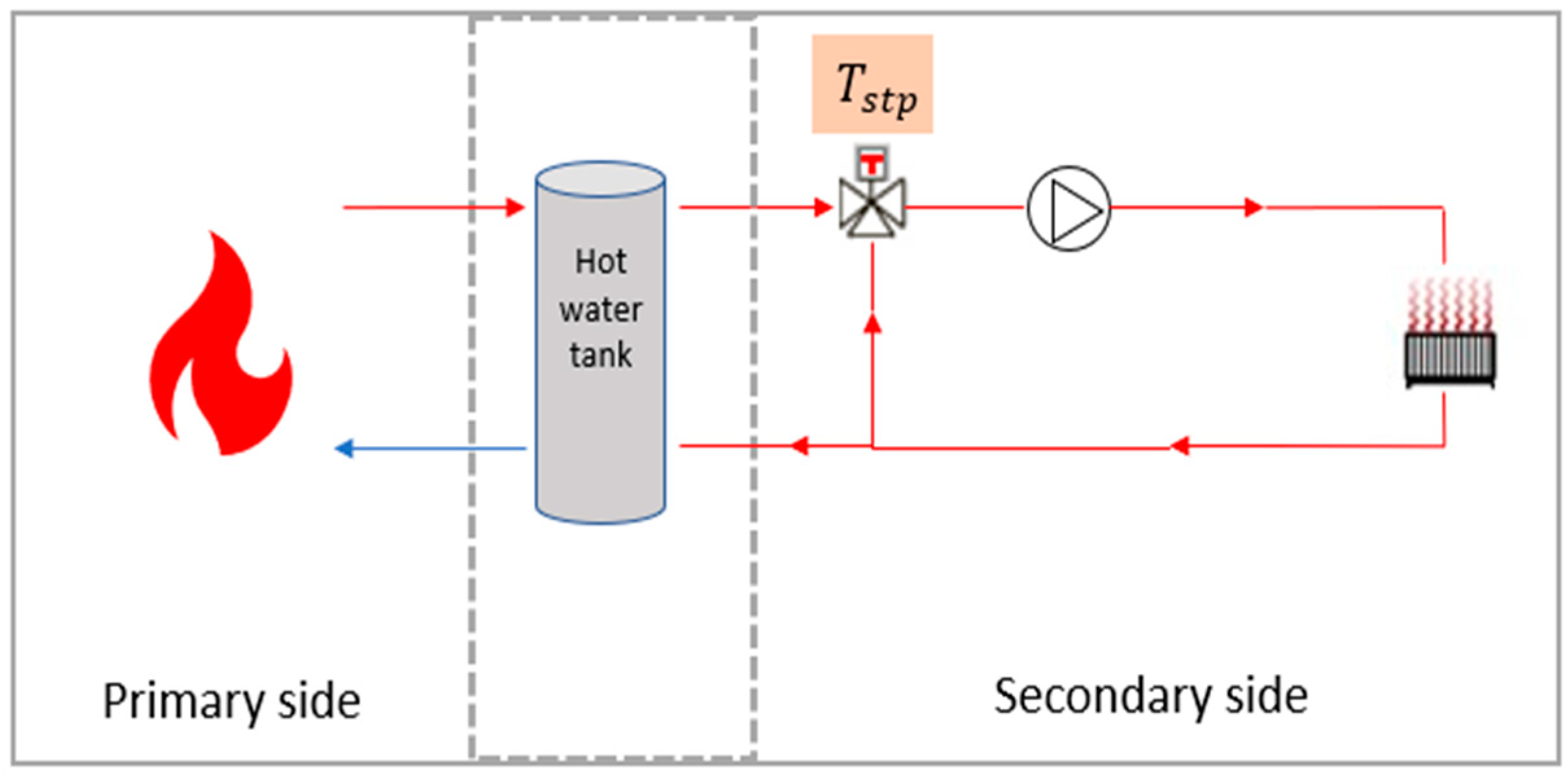
Figure 2 shows the picture of the building that was modeled. It is a commercial building composed of three floors. Referring to standard values for buildings constructed before 2012 [21], the external walls are modeled in brick, with 6 cm of insulation, the floor in insulated reinforced concrete, and the attic insulated with 15 cm of mineral wool. Double-glazed windows are added on both sides of the building. Concerning the heating, the building is heated by a hot water radiators system, which is a very common installation in France. This type of system is often composed of two circuits: a primary and a secondary circuit [35]. Figure 3 shows the modeled heating network. The hot water heating system is based on two interconnected circuits: a primary circuit and a secondary circuit. The primary circuit mainly consists of a gas boiler, whose function is to keep the water in a buffer tank at a high temperature. The secondary circuit, on the other hand, supplies a network of radiators distributed throughout the building. To heat the building, a pump ensures the circulation of hot water in this network. The regulation of the supply water temperature, denoted as $T_{stp}$ in Figure 3, within the secondary circuit is carried out by a three-way valve, which adjusts the mix between the return water from the secondary circuit and the hotter water coming from the buffer tank.

In this paper, a type 526 radiator from the TESS library was used. The radiator surface was adjusted to emit the amount of heat required to heat the building. A constant flow rate was maintained on both sides of the heating network. The system adjusts the opening of the three-way valve based on the flow temperature according to the given setpoint. Thus, the setpoint temperature applied to the control valve governs the entire heating system. Buildings with this type of installation are typically controlled using a single heating curve that sets the supply temperature according to the outdoor temperature. This means that a single setpoint temperature is provided to the valves to regulate the various zones of the building. For this reason, the case study building was modeled as a single zone with a volume of 4968 m³, controlled by a single setpoint temperature. As the authors did not have access to real data for the building, the exact values of the parameters for the heating curve of the reference building were unknown. However, theoretical considerations suggest that the heating curve is adapted to the occupancy scenario, with reduced heating at night and during unoccupied periods.

It is evident that no simple relation exists between the heating power dissipated by the radiators and the setpoint temperature controlling the 3W valve, nor between the setpoint temperature and the energy consumed by the boiler.

The TRNSYS18 simulation was performed at hourly intervals over a full year. Weather data corresponding to northern France, available in the TRNSYS18 software files, were used for the simulation. This file contains weather prediction data over a complete year. The heat provided by the radiators was obviously taken into account, as well as internal gains made by the occupants, if present. An occupancy scenario was defined from 8 a.m. to 6 p.m., Monday to Friday. This is the occupancy level corresponding to our reference building and it specifies the periods of building occupancy and non-occupancy. A ventilation scenario of 0.2 vol/h was also imposed, as well as a low infiltration.

The goal of this work was to determine an optimal hourly sequence of setpoint temperature values for the heating system’s three-way control valve, over a receding prediction horizon. To simulate the building’s response to varying setpoints, changing weather conditions, and occupancy patterns, a random sequence of setpoint temperatures was applied to the control valve in our building model. These values, ranging from 16 °C to 80 °C, were selected based on domain knowledge to ensure their practical relevance and were generated using a uniform random distribution. The objective was to simulate the building’s response to setpoint temperatures that are independent of outdoor conditions. This aligned with the study’s goal of transitioning from conventional heating curves to optimal control sequences for setpoint management. The simulation was run using these random values, generating 8760 records (one record for each hour of the year). These data were then used to model the thermal behavior of the building and heating system.

2.2. Data-Driven Prediction Models

The data used for modeling are simulation data generated by TRNSYS18, so the prediction models detailed in this section were trained using these data. The study deliberately focused on commonly measured variables, despite the availability of many others through TRNSYS18 simulations. Above all, the aim was not to measure and use the supply and the return water temperatures, but instead to model the building’s response to the setpoint temperature imposed on the valve. This is the variable typically used to control this type of system. Thus, five variables represent the initial inputs of the models: setpoint temperature, outdoor temperature, horizontal radiation, indoor temperature, occupancy and gas consumption, noted, respectively, as follows: $T_{cons}$, $T_{out}$, Rad, $T_{in},$ Occ, and $C_{gas}$.

Several research studies have been carried out to model the temperature of a building zone and have shown that the most accurate prediction is obtained by adding historical data measured in the building, i.e., by integrating lagged terms of the variables as input parameters to the model. The number of lags to be used varies from one building to another and has to be studied. It depends on the inertia of each building and on the type of its systems. Fu et al. [36] worked on the prediction of a building’s air-conditioning load and found the best result by taking the values of the previous 48 h of electricity consumption. Mechaqrane et al. [37] also implemented prediction models for building indoor temperature, comparing a linear autoregressive model of indoor temperature with a neural network that takes the building’s past measured data as parameters. They found that a neural network with 3 lagged terms of indoor temperature, 2 of outdoor temperature, 3 of horizontal radiation, and 2 of heating requirements gave the best prediction result with a linear activation function. Ma et al. [29] used LSTM for time series prediction; thus, the future values of indoor temperature were predicted using the past measured values of parameters in the building.

In this paper, the building was modeled based on its historical measured data. Two predictive models were developed: one for forecasting indoor temperature and another for predicting gas consumption. The integration of historical data proved to be helpful when selecting the model structure. Indeed, it allowed for capturing the building’s thermal inertia, thereby significantly improving the accuracy of both models. Several machine learning algorithms were tested, including multiple linear regression, random forest, artificial neural networks, LSTM, GRU models, and support vector machines. In the following sections, only the models that yielded the best performance are discussed, which are ANN and SVM.

Model training was performed on part of the data, while another part was retained to test the model. Normalization was also applied to the data. In order to evaluate the model, besides the coefficient of determination, a prediction error rate was calculated on the test dataset. The model’s coefficient of determination $R^2$, which measures how well the observed data match those fitted, was also calculated. A coefficient of determination close to 1 indicates good model accuracy. Equation (1) shows the formula of $R^2$.

$$R^2=1-{\displaystyle \frac{{\sum }_{i=1}^n{\left(y_i{-\widehat{y}}_i\right)}^2}{{\sum }_{i=1}^n{(y_i-\overline{y})}^2}}$$

(1)

where $y_i$ is the measured value, ${\widehat{y}}_i$ is the predicted value, $\overline{y}$ is the mean of the observed values of y, and n is the number of observations of the test dataset.

Thus, in the presented work, three error metrics were used:

Mean Absolute Error (MAE), calculated as presented in Equation (2), yields the average of the absolute deviations from the observed values.

$$\mathrm{MAE}={\displaystyle \frac{1}{n}}{\sum }_{i=1}^n\left|y_i-{\widehat{y}}_i\right|$$

(2)

The Root Mean Square Error (RMSE) measures the square root of the mean of the square of the errors, as shown in Equation (3):

$$\mathrm{RMSE}=\sqrt{{\displaystyle \frac{1}{n}}{\sum }_{i=1}^n{{(\widehat{y}}_i-y_i)}^2}$$

(3)

The Root Mean Squared Logarithmic Error (RMSLE), which is consistent with ASHRAE’s evaluation method in the Kaggle competition, is mainly used when predictions have large deviations, which is the case with the energy prediction. Also, it measures the relative error between predicted and actual values while being more robust to outliers [38]. It is calculated as shown in Equation (4):

$$\mathrm{RMSLE}=\sqrt{{\displaystyle \frac{1}{n}}{\sum }_{i=1}^n{(log\left({\widehat{y}}_i+1\right)-log(y_i+1\left)\right)}^2}$$

(4)

Concerning MAE, RMSE, and RMSLE, the smaller the values of these errors are, the better the model is.

2.2.1. Artificial Neural Network for Indoor Air Temperature

The first machine learning model developed was an artificial neural network. The ANN was chosen because it has proven its efficiency in many building studies, especially in the prediction of indoor air temperature. It provided the best results in [6,37,39,40,41]. Also, numerical optimizations using a combination of artificial neural network and genetic algorithm can be efficient for building applications, which can save a significant amount of computational time [42].

An artificial neural network is formed from layers of interconnected artificial neurons, whose role is to find the best relation between input and output. This relation is defined by an activation function found in each neuron, and by coefficients. These coefficients are the synaptic weights of the neural network. During learning, the neural network performs several iterations to adjust the weights in a way that minimizes the error between the predicted value $\widehat{y}$ and its real value y. In this paper, the ANN model was used to predict the building’s indoor temperature at the next hour, denoted as $T_{in}$(t).

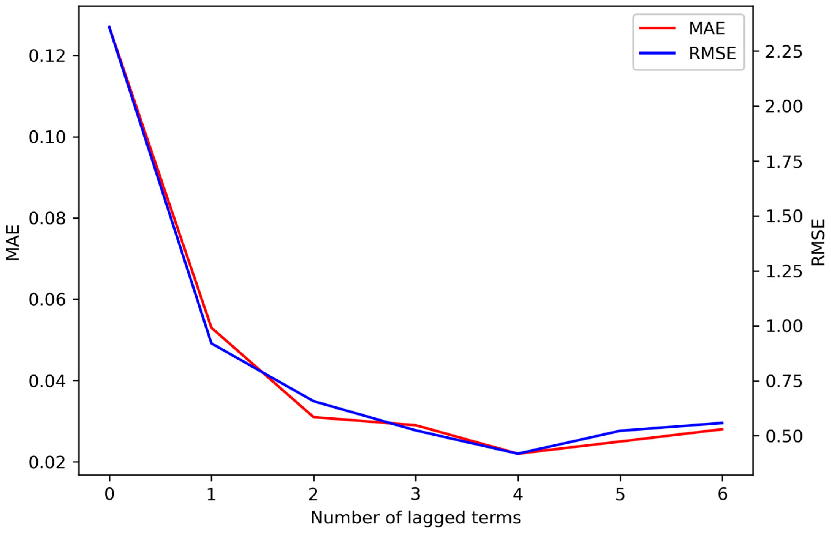
The main difficulty with neural network models is choosing the network architecture, that is, the number of layers and neurons. Several models were trained by varying the number of lagged terms n and the number of layers and neurons in the network and testing the activation function «linear», «softplus», and «sigmoid». By lagged terms, we refer to variables observed or recorded at a specific number of hours prior to the current time. Results show that the «softplus» gives the best prediction for this case study, consistently yielding the smallest error and the highest coefficient of determination compared to other activation functions in models trained with the same number of lagged terms. To avoid overloading the table, the results of ANN with «softplus» only are presented in

Table 1. Error metrics of the trained ANN with “Softplus” activation function and different lag numbers.

Number of Lagged Terms	MAE	RMSE	${\mathit{R}}^2$
0	0.14	2.27	0.14
1	0.053	0.97	0.84
2	0.031	0.6	0.93
3	0.04	0.57	0.95
4	0.022	0.42	0.97
5	0.025	0.52	0.96
6	0.028	0.55	0.95

.

Figure 4 shows the evolution of the MAE with varying numbers of lags, ranging from 0 (no historical building data considered) to 6 lags. Table 1 shows that the prediction error gradually decreases as the number of lagged terms increases, and remains in this trend up to 4 lagged terms. Beyond this point, the error tends to increase again. Therefore, the model that appears to be optimal for predicting indoor temperature in this study is an artificial neural network with n = 4 lags, one hidden layer with 50 neurons, and a nonlinear activation function, the «softplus» function, shown in Equation (5).

$$f\left(x\right)=log(1+\mathrm{e}\mathrm{x}\mathrm{p}(x\left)\right)$$

(5)

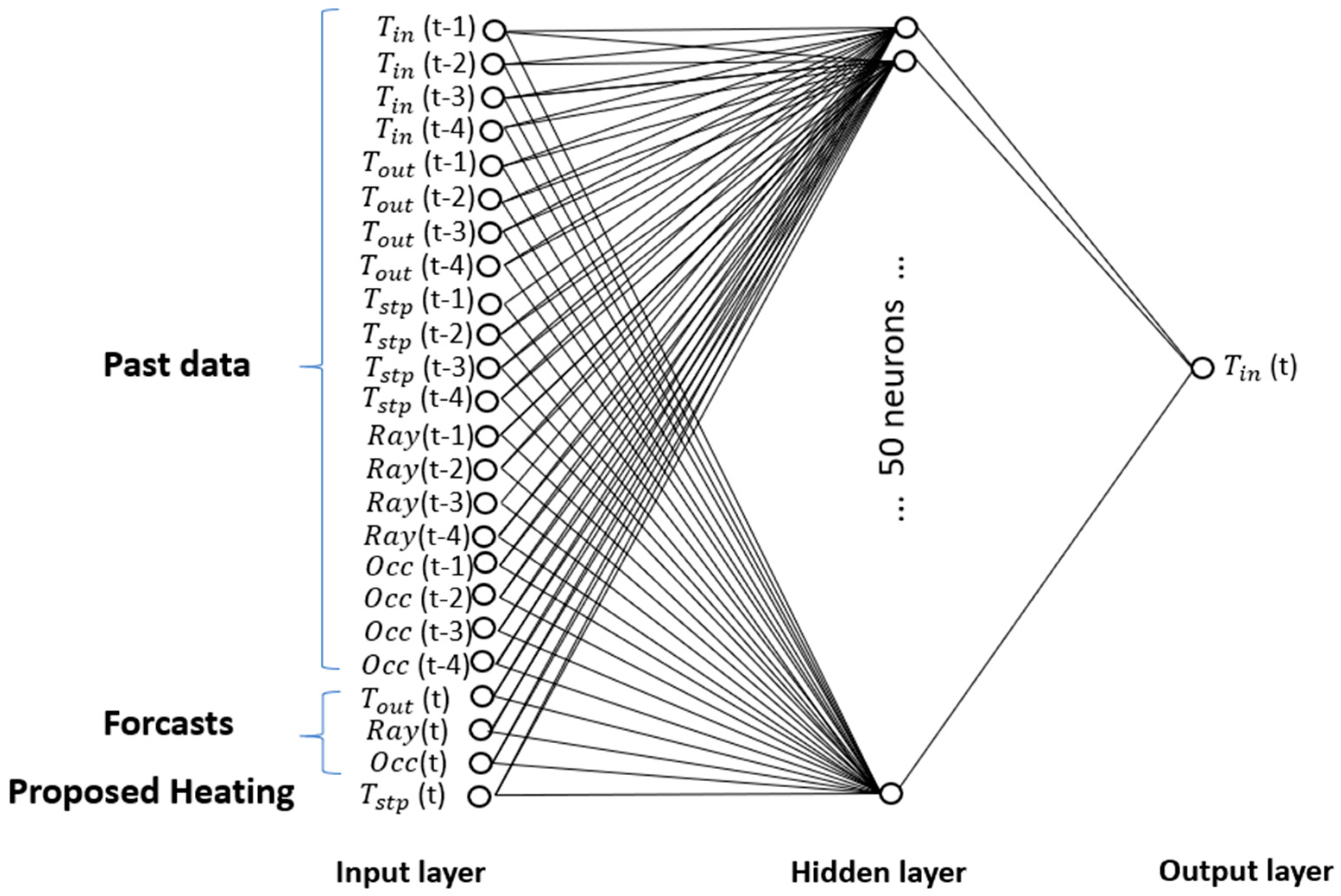
The topology of the adopted model is illustrated in Figure 5. The model inputs are the historical measurements of indoor temperature, outdoor temperature, horizontal radiation, occupancy, and setpoint temperature, respectively, noted as $T_{in}$, $T_{out}$, Rad, Occ and $T_{cons}$ from time t − 1 to t − 4. Additionally, the model relies on forecasts for outdoor temperature, solar radiation, and occupancy (at time t), as well as the setpoint temperature value proposed by the genetic algorithm $T_{stp}$(t). Consequently, the input layer of the neural network comprises 24 neurons: $T_{in}$(t − 1), $T_{in}$(t − 2), $T_{in}$(t − 3), $T_{in}$(t − 4), $T_{out}$(t − 1)$,T_{out}$(t − 2), $T_{out}$(t − 3), $T_{out}$(t − 4), Rad(t − 1), Rad(t − 2), Rad(t − 3), Rad(t − 4), Occ(t − 1), Occ(t − 2), Occ(t − 3), Occ(t − 4), $T_{stp}$(t − 1)$,T_{stp}$(t − 2), $T_{stp}$(t − 3), $T_{stp}$(t − 4), $T_{out}$(t), Rad(t), Occ(t), $T_{stp}$(t). The error measurements of the adopted model are provided in

Table 2. Error metrics for ANN model.

Model 1	${\mathit{R}}^2$	RMSE	MAE
ANN	0.97	0.42	0.022

.

2.2.2. SVM for Gas Consumption Prediction

The second model is designed to predict the gas consumption of the boiler. As previously explained, there is no straightforward relationship between the control setpoint and gas consumption. To solve this task, several models are trained with the aim of finding the most accurate possible model, always with the available data. This raises several challenges regarding the choice of model and the choice of the number of lagged terms for any variables. The initial variables are therefore the same: $T_{in}$, $T_{out}$, Rad, Occ and $T_{cons}$.

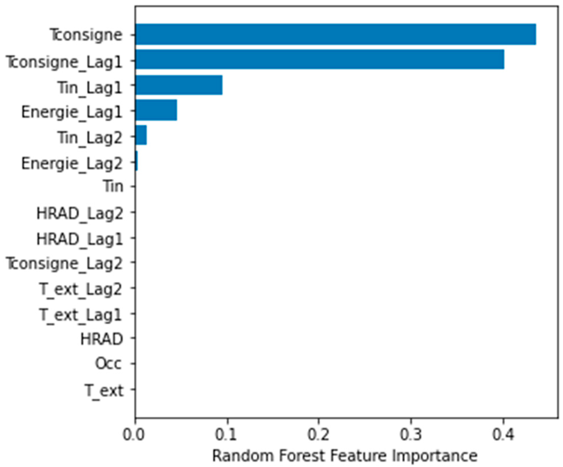
In this study, random forest was used to calculate the importance of the characteristics of the model and then help in removing unnecessary variables. Random forest is a combination of decision trees. It improves the performance of a single tree by combining the randomization in the selection of partitioning data nodes in the construction of a decision tree. Hence, random forest determines feature importance by measuring each feature’s contribution to reducing impurity (like Gini impurity or MSE) across all splits and trees in the ensemble, with higher reductions indicating more important features [43]. Figure 6 reveals the features’ importance by a random forest with n = 2 lagged terms. It appears that taking measurements more than 1 step back does not lead to a better prediction. The results of the trained models, using different number of lags of the variables show that the best prediction can be performed using only four variables: $T_{stp}\left(t\right)$, $T_{in}$(t − 1), $C_{gas}$(t − 1), $T_{stp}$(t − 1). Using these features, a support vector machine (SVM) model gives the most accurate prediction in this study.

SVM is a supervised machine learning algorithm that aims to find an optimal boundary between possible outputs by maximizing the separation margins between data points based on their responses. This transformation of inputs is achieved using the machine’s kernel function. In this study, Support Vector Regression (SVR) (a type of support vector machine) was used to analyze data for regression analysis. SVM has been commonly used for the energy prediction in buildings [30,33,36,44,45].

In this study, the radial basis function (RBF), represented in Equation (6), was chosen due to the broad and nonlinear characteristics of the dataset [46].

$$K_{RBF}\left(x-x^{\prime }\right)=exp(-\gamma x-{x^{\prime }}^2)$$

(6)

where γ is a parameter to determine the distribution of the kernel, and $x$ − $x^{\prime }$ is the Euclidean distance between the set of points [30].

The adopted model is also based on the lag terms n = 1 of the building’s indoor temperature, gas consumption, and setpoint temperature value $T_{stp}$(t) proposed by the genetic algorithm. The output of this model is the estimated gas consumption at time t. Among several models tested using the selected features, SVM gives the best prediction accuracy. The error measurements of the adopted model are provided in

Table 3. Error metrics for SVM model.

Model 2	${\mathit{R}}^2$	RMSLE
SVM	0.83	2.9

.

2.3. Optimization

As mentioned previously, the objective of this study is to identify a sequence of 24 hourly setpoint temperatures for the heating system that balances thermal comfort and energy consumption. Therefore, a multicriteria optimization problem arises. Genetic algorithms are well suited for this type of problem [47]; in particular, these algorithms have gained prominence in the optimization of building thermal systems [48].

Genetic algorithms are inspired by the process of natural selection and evolutionary biology, where an individual is represented by a chromosome composed of genes containing hereditary traits. The process begins with a population of potential solutions represented by individuals, often in the form of binary strings encoding possible solutions. In this case study, the initial population consists of setpoint temperature scenarios, and each scenario comprises 24 temperature values. Moreover, each setpoint temperature value is encoded with 6 bits, with each individual represented by 144 bits. Since each bit can take 2 possible values (0 or 1), the number of possible solutions for each proposed temperature scenario reaches more than 2.2 × ${10}^{43}$ solutions.

The focus of this study is on the setpoint temperature of the water supplying the radiators in the secondary circuit, rather than on optimizing the boiler’s operation. Thus, the setpoint temperature values that can be chosen by the genetic algorithm range from 16 °C to 70 °C. The fitness of each solution in addressing the given problem is evaluated based on a predefined objective function. The individuals then go through genetic operations, including selection, crossover, and mutation. During selection, only the fittest solutions are chosen to become parents for the next generation. The number of generations is determined by the number of iterations. In crossover, genetic information is exchanged between parents to create offspring that exhibit a combination of their characteristics. Mutation introduces random changes in the genetic information of the offspring. This cycle of selection, crossover, and mutation repeats over multiple generations, gradually improving the overall fitness of the population and converging towards optimal solutions, or those with the best objective function scores.

In this study, the comfort score is simply estimated as a function of indoor air temperature, as in most cases [17,21,27,29]. This is because the temperature is an easily measurable parameter, compared to other parameters such as air speed or relative humidity which play a role in the notion of comfort. Therefore, ranges of comfort temperatures are defined for the genetic algorithm to adhere to. The details of these temperatures are shown in

Table 4. Comfort temperature range during occupation/non-occupation shifts of the week.

Shift	Occupation	Target Temperature
Weekday [08 h–18 h]	Yes	[20–22 °C]
Weekday [19 h–07 h] Weekend [00 h–23 h]	No	≥15 °C

. The objective is to maintain an indoor temperature between 20 °C and 22 °C during occupied hours (from 8 a.m. to 6 p.m. on weekdays). The comfort score of any solution that results in an indoor temperature outside this range will be penalized. Similarly, during unoccupied hours, temperatures below 15 °C are penalized. This approach aligns well with conventional control practices in real life, where similar steps are taken to prevent excessive temperature drops and the associated inefficiencies in recovery.

Figure 7 details the calculation of the comfort score of each hour of the day: if the building is in its occupation period (as shown in Table 4) and the indoor temperature is below the lower limit of the defined comfort temperature range, the difference between these two temperatures is added to that score. Similarly, if the indoor temperature exceeds the upper limit of the defined comfort temperature range, the difference between these two temperatures is added to the comfort score. However, if the indoor temperature is within the defined comfort temperature range, the score is not penalized. The calculation is performed similarly during non-occupation hours; if the temperature drops below 15 °C, the score is penalized.

In this study, the comfort and gas consumption scores are normalized to facilitate balancing their weights effectively. For the comfort score calculation, an individual score is computed for each of the 24 h (as shown in Figure 7). These hourly scores are then summed up and divided by 24, as the maximum possible score for a single hour is approximately 1, resulting in a normalization factor of 24 × 1, as in Equation (7), so the value of the comfort score ranges between 0 and 1:

$${score}_{comfort}={\sum }_{\mathrm{j}=1}^{24}\left({score}_{comfort\left(j\right)}\right)/24$$

(7)

Concerning the consumption score, it represents the gas consumed over 24 h, as shown in Equation (8). It is normalized by dividing the summation by the maximum value of gas consumption over 24 h, so the value of the consumption score falls between 0 and 1.

$${score}_{consumption}={\sum }_{\mathrm{j}=1}^{24}{C}_{gas\left(j\right)}/C_{gas\_max}$$

(8)

Since the objective of this study is to achieve a trade-off between comfort and consumption, the score for each solution is calculated by adding the score of comfort to the score of consumption. The final score is thus calculated according to Equation (9). The goal is to minimize the final score over a 24 h period.

$${score}_{final}=\omega \times {score}_{comfort}+\left(1-\omega \right)\times {score}_{consumption}$$

(9)

With this definition of the comfort final score (${score}_{final}$), the strategy enables users to define the priority of comfort relative to energy consumption. A lower value of ω places greater emphasis on consumption, while a higher value prioritizes comfort. This way, with both sub-scores being normalized, theoretically, ω can tolerate values between 0 and 1. Thus, it becomes evident that ω = 1 only considers comfort and ω = 0 only considers consumption. But from a practical perspective, ω values should avoid extreme settings. Specifically, ω = 0 would result in the algorithm deactivating the system, thereby eliminating comfort entirely, which is inconsistent with the intended goals of the strategy. Conversely, ω = 1 would prioritize comfort to the exclusion of energy efficiency, potentially leading to excessive energy consumption, which similarly contradicts the strategy’s overarching objectives.

The choice of the value of ω is left to the discretion of the building manager. The weight ω specifies the priority level of comfort relative to consumption, meaning ω can be adjusted to favor one score over the other. Since the comfort score and the energy consumption score are qualitatively different metrics, they cannot be rigorously balanced against one another. In this study, the authors selected a value of ω = 0.5, a midpoint of the [0, 1] interval, to serve as a neutral baseline, in order to combine the two criteria in one objective function. We proceeded under the hypothesis that this value aligns with the overarching aim of the strategy to optimize system performance while maintaining a practical equilibrium between the competing priorities. Therefore, the results presented in this article were obtained with a weight of ω = 0.5.

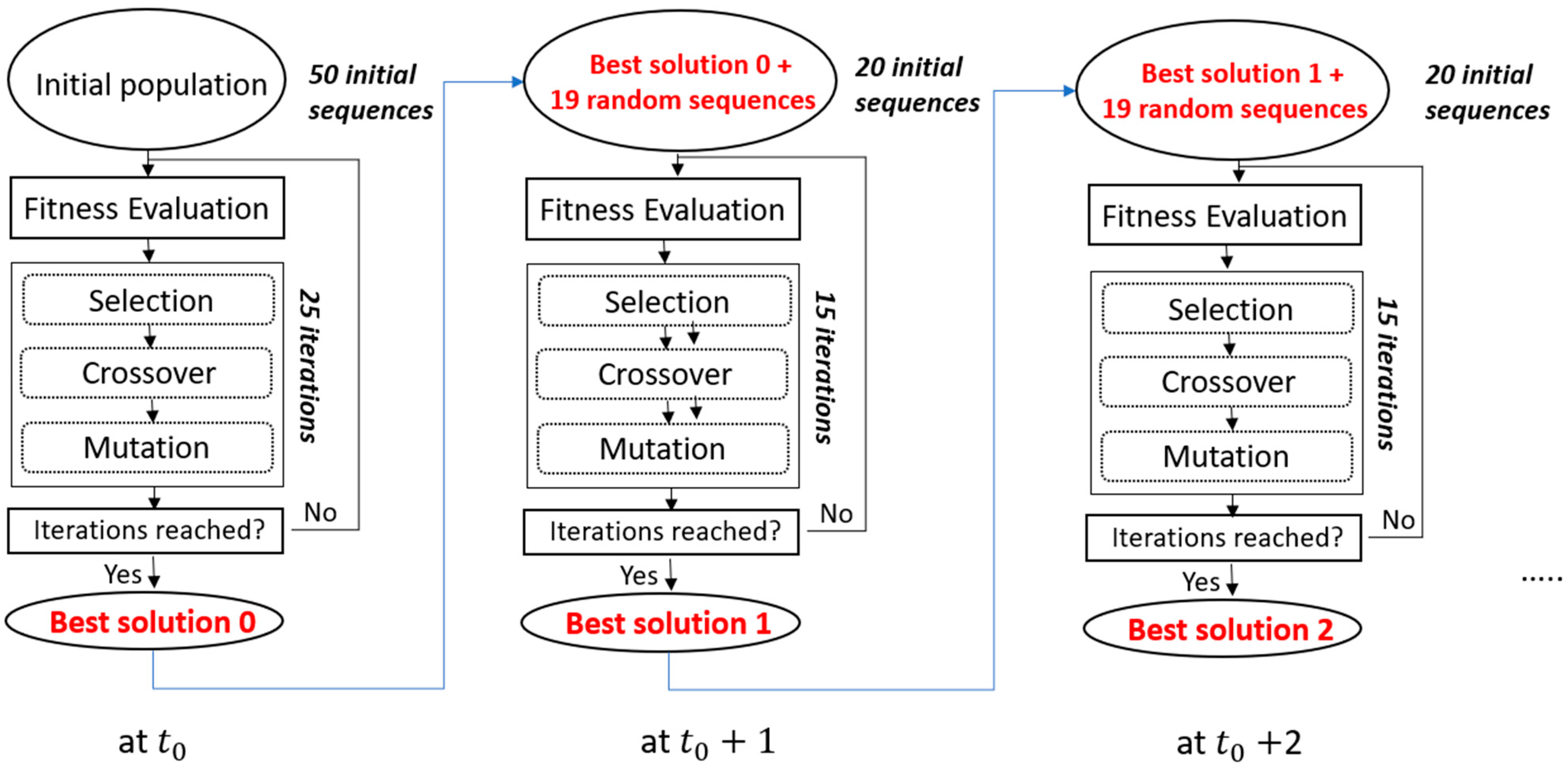
As explained, the optimization using the genetic algorithm is initiated every hour in an infinite loop (loop 3 of the methodology as explained in Section 2), enabling a receding horizon. Each iteration of this loop represents the calculation of an optimal sequence for 24 h. At time $t_0$, the GA finds an optimal solution, adhering to the defined number of solutions for the initial population and the number of iterations to be performed. In this study, we focused on reducing the computational complexity by helping the genetic algorithm find the best solution at time $t_0$ + 1 by injecting the best solution found at the first optimization ($t_0$). The process is explained in Figure 8. During the second iteration, i.e., at time $t_0$ + 1, the GA can use the previous solution, including it in the new initial population of 20 solutions instead of 50. In addition, the GA performs 15 iterations instead of 25, thereby reducing execution time while maintaining the efficiency of the process (more details are presented in Section 3). Therefore, the number of sequences is limited to 50 for the first iteration of the receding horizon loop (loop 3), and then reduced to 20 for the remaining 47 iterations in this case study (since the loop turns for 48 h).

3. Results

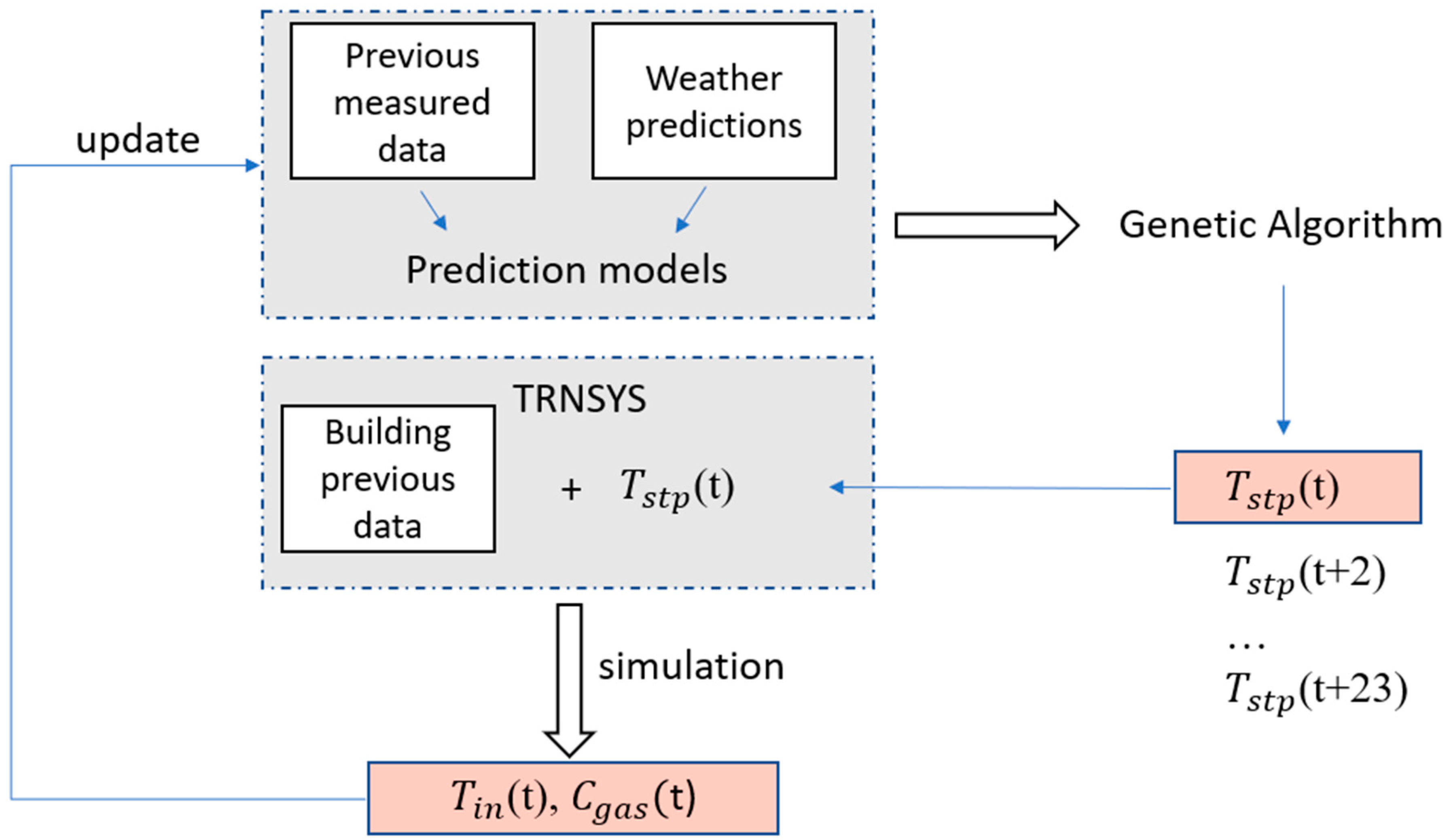
In this study, the first loop of the proposed MPC represents the prediction of indoor temperature and gas consumption over a 24 h horizon, while the second loop denotes the optimization process of the setpoint temperature. Concerning the third one, it represents the receding horizon where the prediction and the optimization are performed at each timestep (every hour), for the next 24 h, in order to adjust the heating scenario if needed. In real-world scenarios, the third loop operates continuously from the moment the strategy is activated until it is deactivated. This means that the forecasting horizon advances incrementally on an hourly basis throughout the duration of the strategy’s implementation. However, in this study, to reduce computational effort and time, the authors chose to validate the strategy by running it for a fixed duration of 48 h loops, applied to 10 randomly selected days. The computation of the optimal solution for one timestep, if the loop can range from 10 to 40 min, is carried out using a relatively high-performance machine (DELL PRECISION 3581, with a 13th Gen Intel Core i9-13900H processor, 64 GB of RAM, and a 64-bit architecture), making it challenging to perform large-scale calculations, such as those spanning an entire year.

The proposed MPC strategy was validated on the modeled building using TRNSYS18. Figure 9 explains the mechanism of this loop. At each iteration, the first setpoint temperature ($T_{stp}$(t)) of the proposed 24 h scenario is applied to the heating system of the simulated building model in TRNSYS18 as a control signal. This allows for the collection of output data, including the indoor air temperature and gas consumption associated with the specified heating setpoint. The simulation is then executed using the building’s historical data, maintaining consistent initial conditions for both the prediction process and the simulation, up to the considered timestep. Once the simulation on TRNSYS18 is performed, the output values of indoor temperature and energy consumption ${(T}_{in}$(t) and $C_{gas}$(t), respectively) are passed to update the dataset used for the prediction and optimization processes at the next timestep. This study was conducted in hourly steps, i.e., one timestep is equal to one hour.

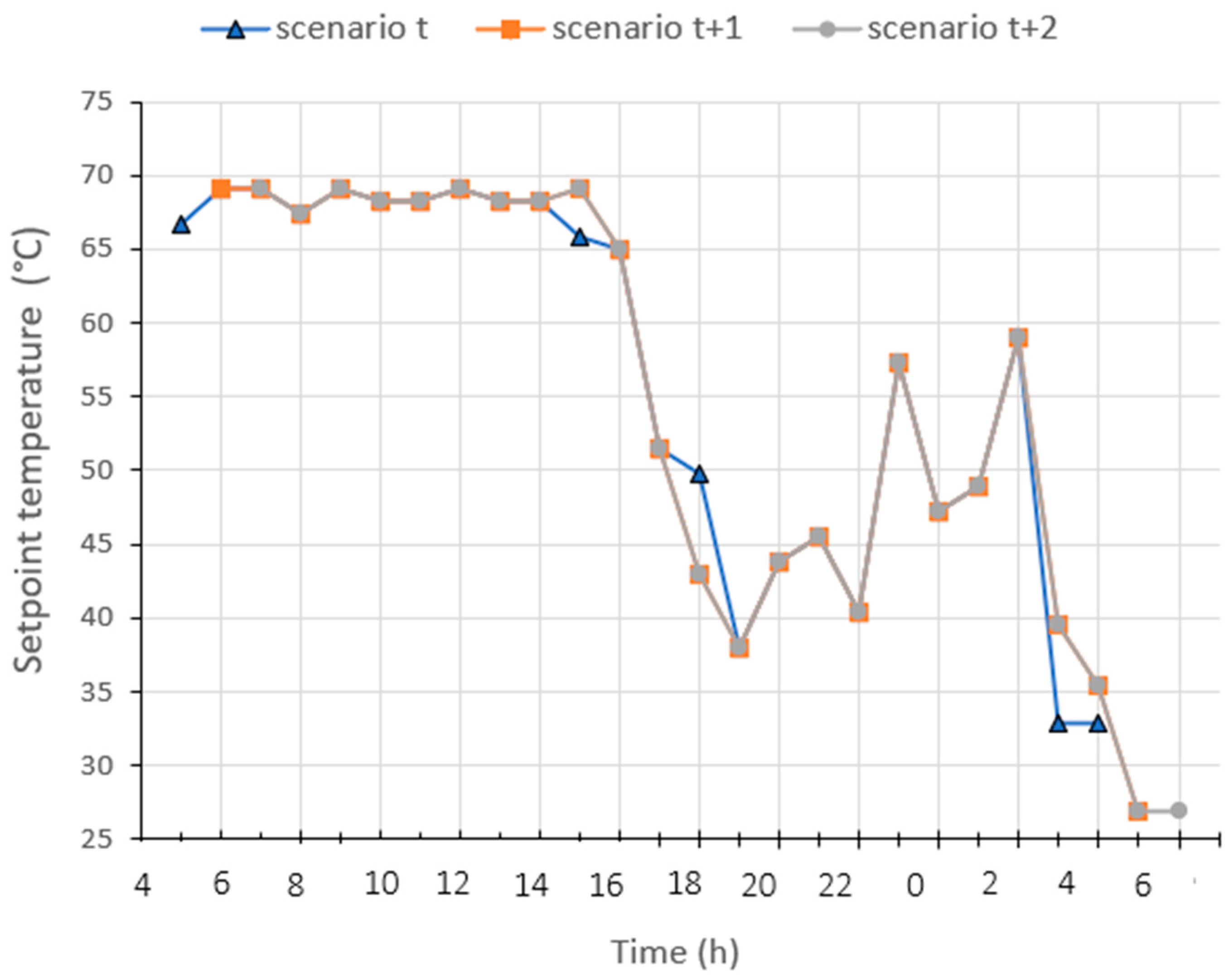
As explained in Section 2, at each timestep, the genetic algorithm attempts to find a solution that best accommodates changes or uncertainties in weather and occupancy. Figure 10 shows an example of evolution of the heating scenarios during three consecutive iterations (from the timestep t at 5 a.m. (scenario t), to scenario t + 1 at 6 a.m., and scenario t + 2 at 7 a.m.). The heating scenario dynamically adjusts to explore improved solutions that enhance comfort while incorporating updated values. This can be more explicit in real-life application, where potential weather or occupancy changes may occur. 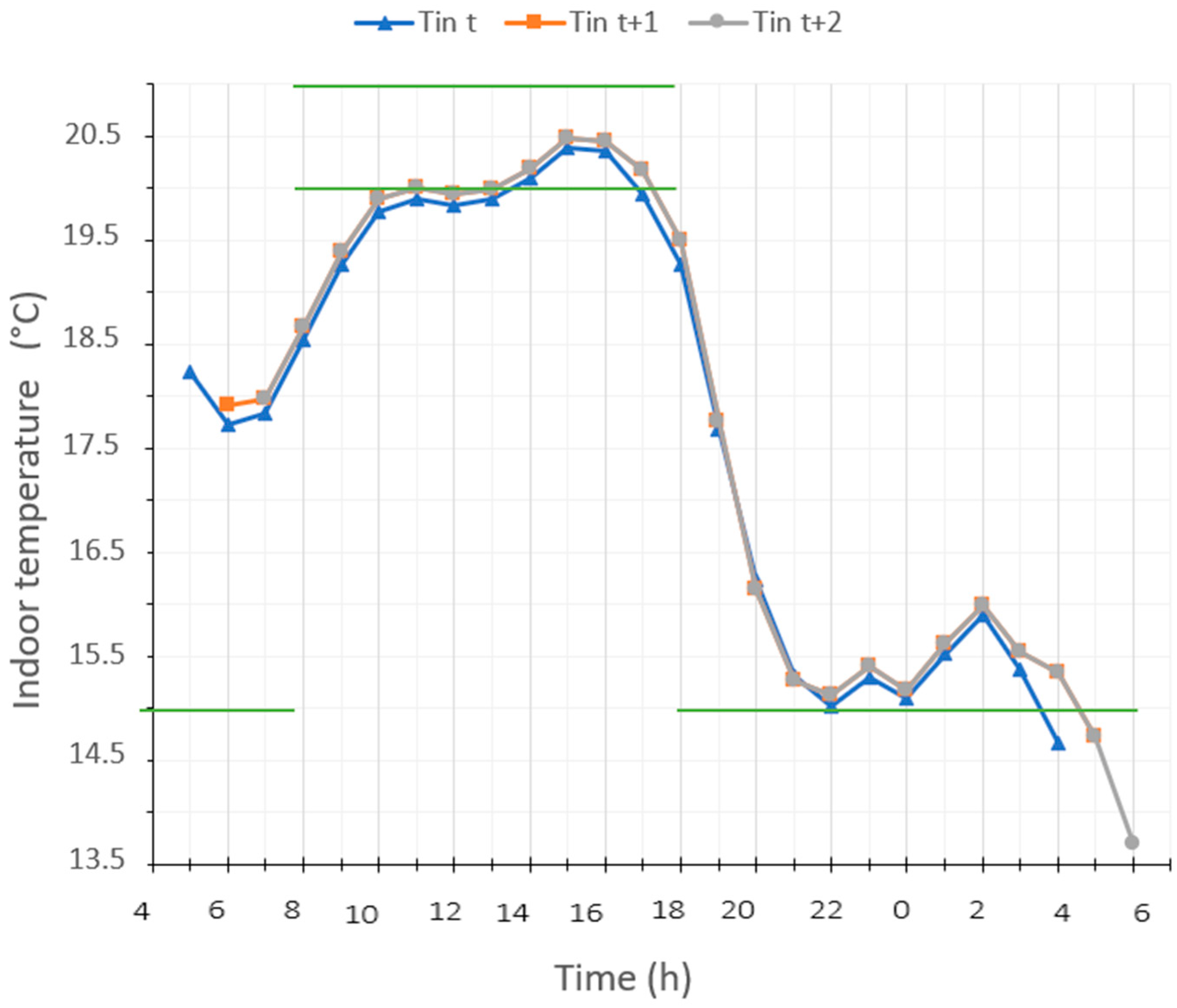Figure 11 shows the indoor temperature that results from each heating scenario presented in Figure 10. The adjustment of the scenario at t + 2 raises the indoor temperature a bit more to try to reach the comfort range temperatures during the occupancy period.

In order to validate the performance of the strategy, 10 random days were selected throughout the heating period. It is important to clarify that these are independent tests. For each of these days, the implementation of the MPC strategy was initiated 24 h in advance to avoid the transition phase between the conventional control strategy and the predictive control strategy. The changes in indoor temperature and gas consumption over the last 24 h of each period were used to calculate the scores. The calculation was thus launched in a 48 h receding horizon loop. That means that 48 iterations of loop 3 were performed for every selected day. The optimization starts at the first timestep t, calculating the 24 values of setpoint temperatures for the next 24 h, considering the next 24 h occupation scenario and weather forecasts. Then, at the next timestep, the calculation of the heating scenario is repeated for the 24 next ones, and so on, for 48 iterations. 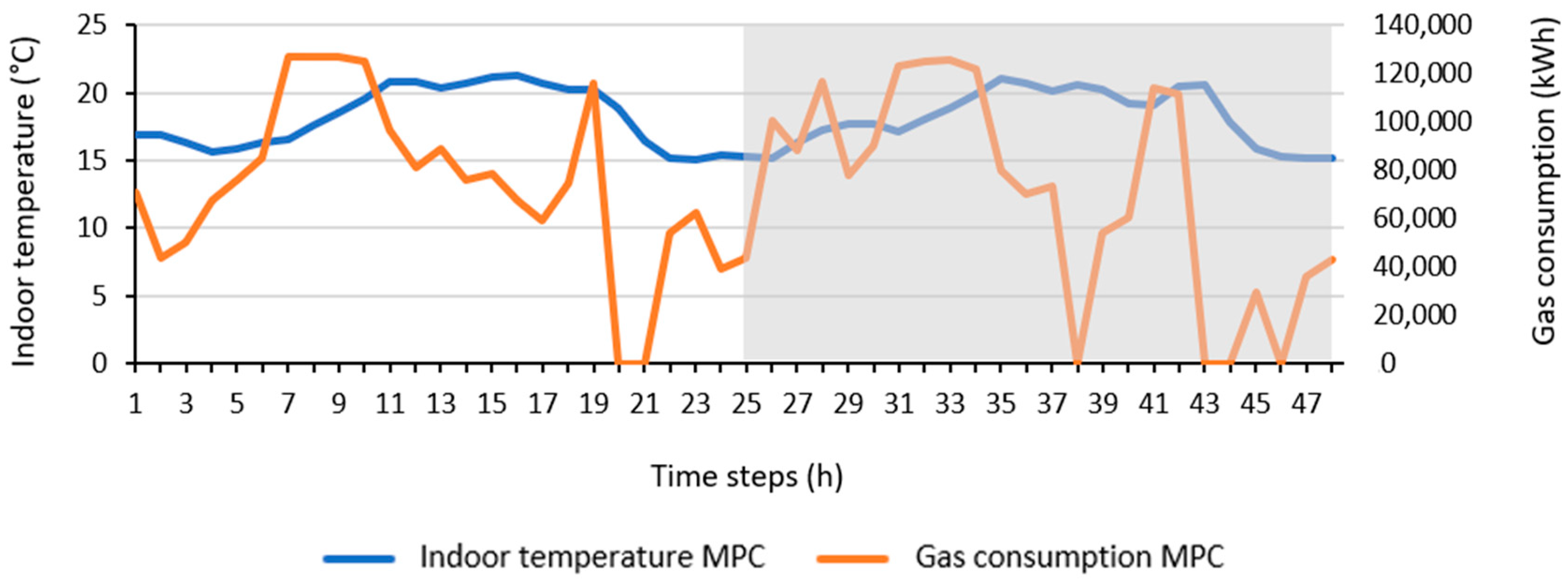Figure 12 shows an example of indoor temperature and gas consumption that result from the MPC strategy applied to 1 selected test day, over 48 h. Only the values of the second day were used to evaluate the applied strategy (the part selected in the grey frame on the graph).

Values of indoor air temperature and energy consumption from the last 24 h were compared to those simulated using a conventional control strategy for the heating system of the same building. This conventional control operates based on a heating curve, a function of the outdoor temperature. The parameters of this heating curve were carefully chosen to ensure an indoor temperature between 20 °C and 22 °C during occupation hours (8 a.m. to 6 p.m.). The heating setpoint temperature starts to increase at 6 a.m. (2 h before the occupation to guarantee a comfort temperature at 8 a.m.), with a night-time setback also implemented. The heating curve was optimally adjusted to provide a credible reference strategy. In other words, the baseline method with which we compared our strategy is already a fairly energy-efficient heating curve, and a heating cutdown is carried out during the night. Figure 13 shows the indoor air temperature in the building, with heating based on the selected heating curve over the course of a week. It is clear that it takes hours to reach a comfortable temperature. The proposed MPC aims to avoid this delay. The results presented in this section correspond to the comparison of the strategy with this selected conventional heating strategy.

Since the aim of the strategy is to balance energy consumption and thermal comfort, the comparison is based on two scores: a comfort score and an energy consumption score. The MPC strategy aims to minimize the final score, which is the sum of both scores, as defined in Equation (9).

Table 5. MPC vs. RBC for the 10 days tested.

Day	Average Solar Radiation (W/m2)	Average Outdoor Temperature (°C)	Comfort Score MPC	Comfort Score RBC	Consumption Score MPC	Consumption Score RBC	Final Score MPC	Final Score RBC	Energy Savings (%)
1	76.2	3.3	0.18	0.18	0.76	0.81	0.47	0.5	6.2
2	34.1	8.2	0.14	0.15	0.4	0.57	0.27	0.36	29.8
3	20.6	−0.6	0.16	0.15	0.62	0.64	0.39	0.39	3.1
4	27.4	7	0.27	0.18	0.39	0.55	0.33	0.36	29
5	23.9	3	0.17	0.14	0.64	0.71	0.4	0.42	9.9
6	38.2	0	0.11	0.13	0.73	0.78	0.42	0.45	6.4
7	5.4	3.3	0.23	0.13	0.65	0.7	0.44	0.42	7.1
8	40.7	3.1	0.37	0.14	0.61	0.69	0.49	0.41	11.6
9	85.1	3.7	0.12	0.29	0.54	0.67	0.33	0.47	19.4
10	31.7	0	0.14	0.15	0.72	0.78	0.43	0.46	7.7

shows the results of both control methods over ten randomly selected days, representing different weather conditions (varying outdoor temperatures, solar radiation). The control using the baseline heating curve is abbreviated as RBC (Rule-Based Control). The calculation is performed over 48 hourly steps for each day as mentioned, meaning that during these 48 h, the optimization is reinitiated every hour with a 24 h horizon each time. The scores presented in Table 5 are calculated on the second day (the last 24 h) to ensure that the strategy is evaluated based on a steady-state regime.

Table 5 shows the comfort scores of both strategies in every selected test day. We can see that, in almost all cases, the MPC comfort scores are equal or lower than the RBC scores (days 1, 2, 6, 9, and 10), while an energy consumption reduction is proved by the MPC strategy in all presented days. Here, it is worth mentioning that, since there is a comfort range of temperature that is defined for the occupation and the unoccupancy period as well, the comfort score could be penalized for the violation of both. That means that, even during unoccupancy, if the temperature drops below 15 °C (Table 4), the comfort score will increase; however, this does not imply that the building occupants feel discomfort.

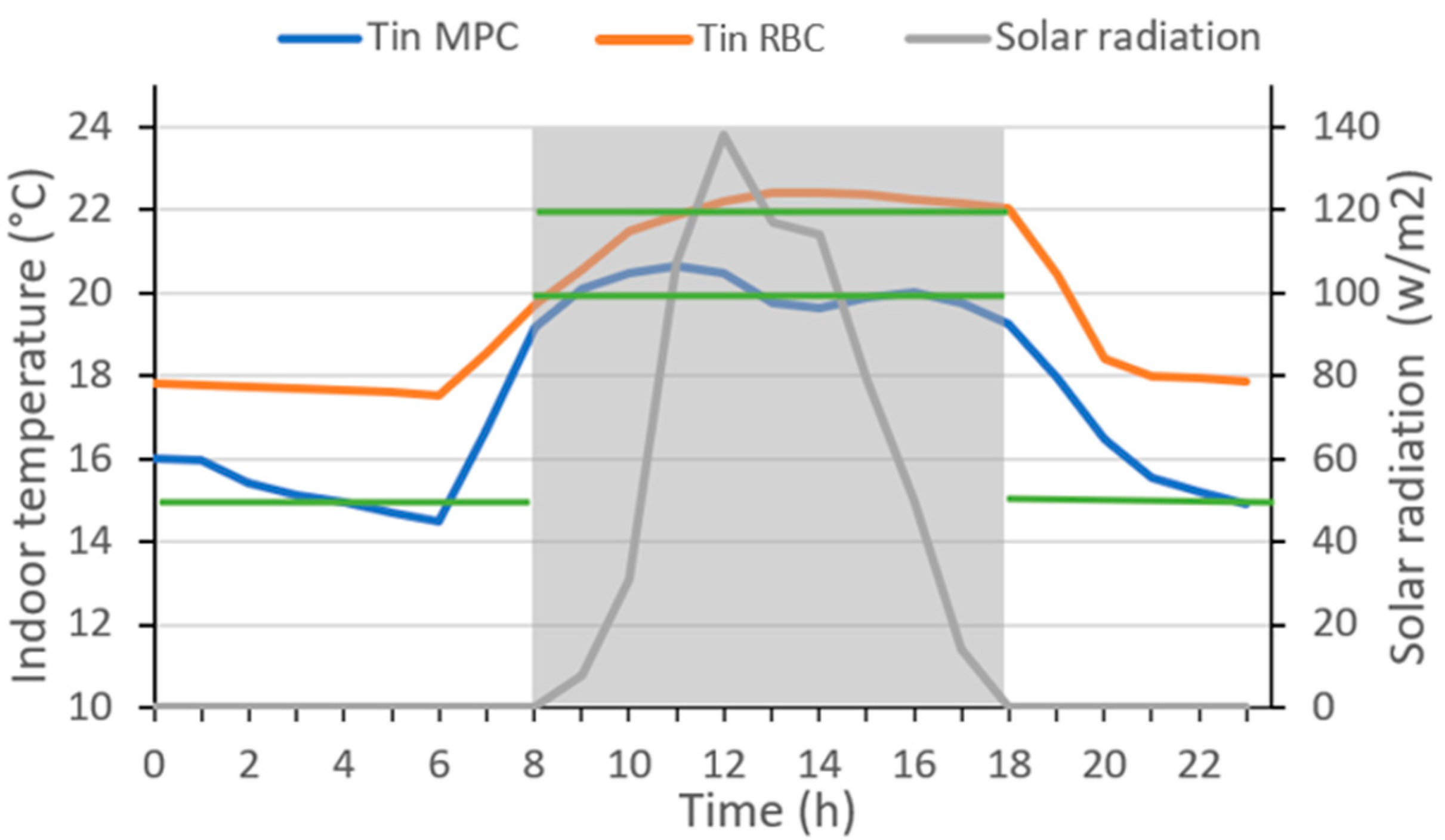
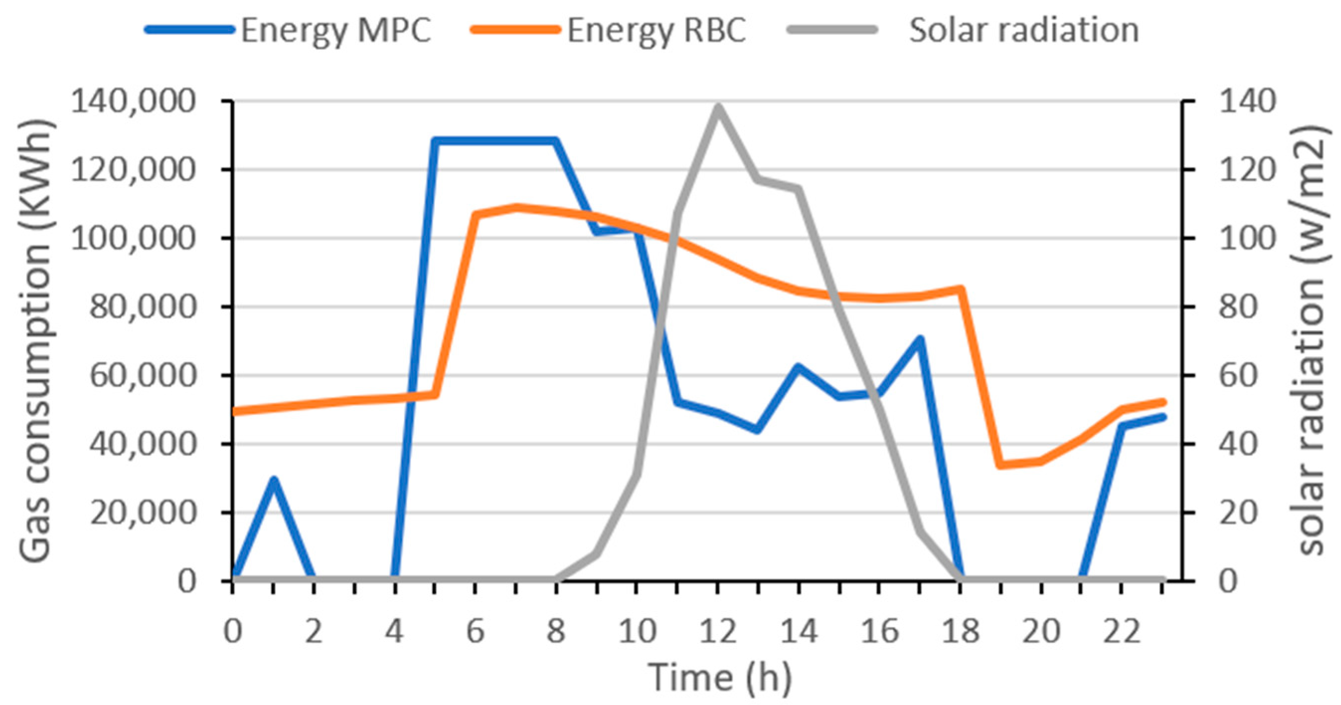
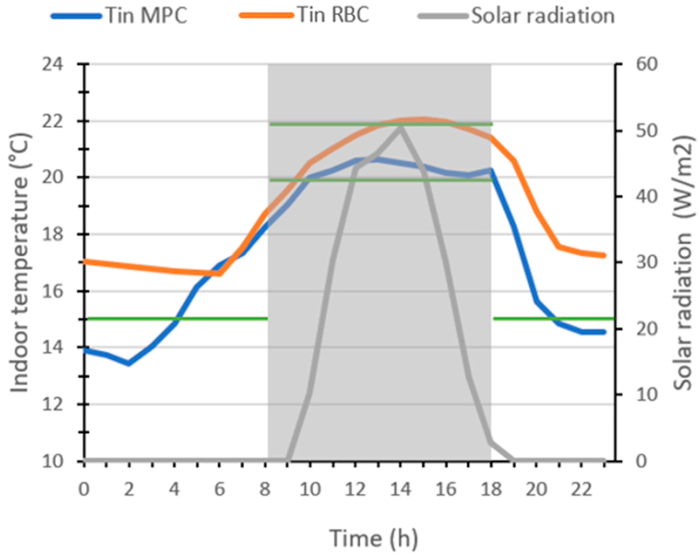
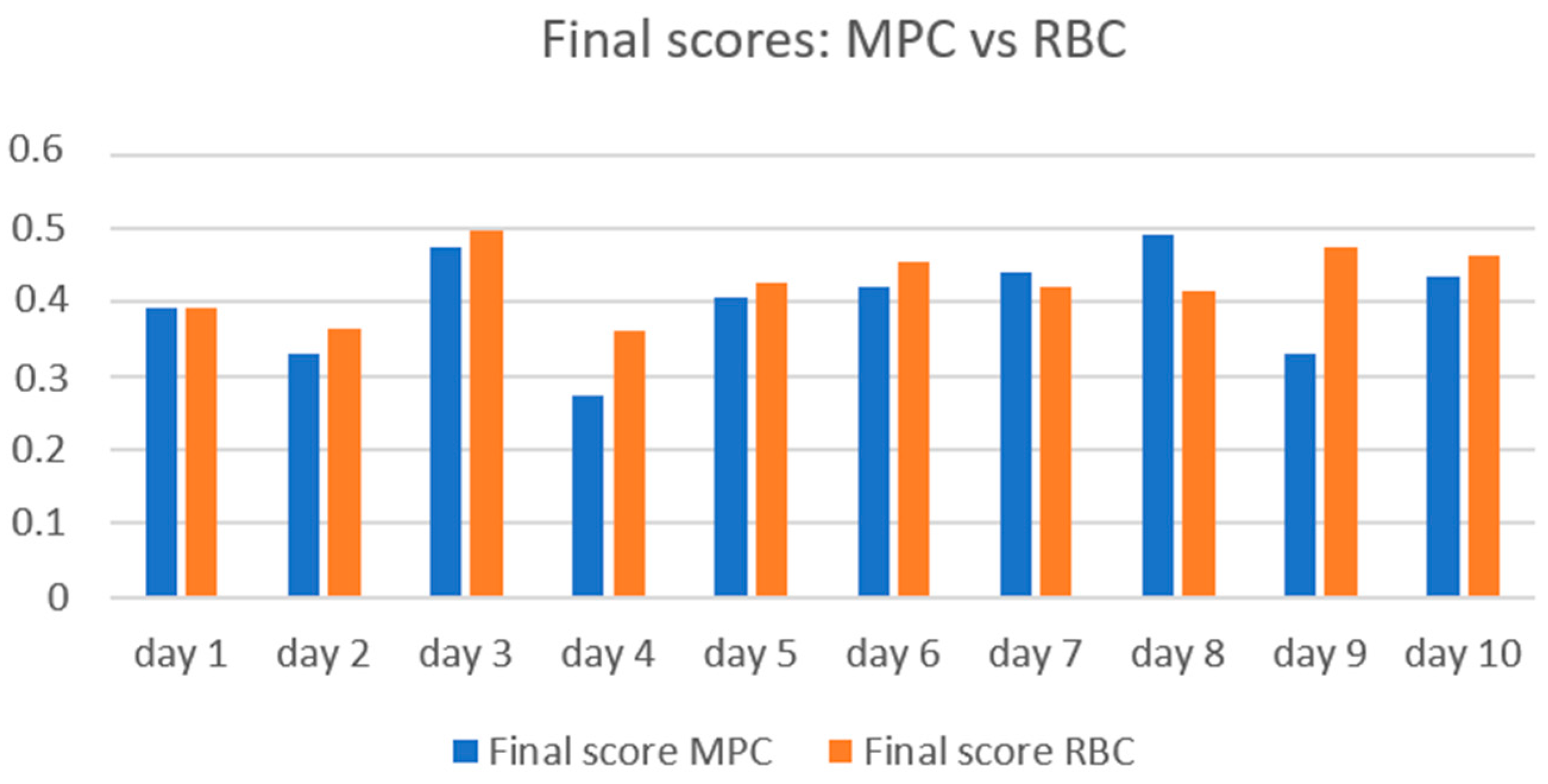
Figure 14 and Figure 15 compare, respectively, the indoor temperature and the energy consumption of both strategies on day 4 presented in Table 5. The MPC strategy was able to anticipate the solar radiation expected during the day, to keep the indoor temperature within the comfort range (between 20 °C and 22 °C) during occupancy hours (grey frame). The results show lower gas consumption in the case of the MPC strategy, compared to that of the RBC where the indoor temperature exceeded the defined comfort range (above 22 °C). The comparison of the final scores over the 10 selected days is visualized in Figure 16. It shows that the MPC strategy outperforms the conventional strategy in most cases (lower final scores for MPC), except for days 7 and 8. This is due to the MPC comfort score which is higher than that of the RBC during these two days. 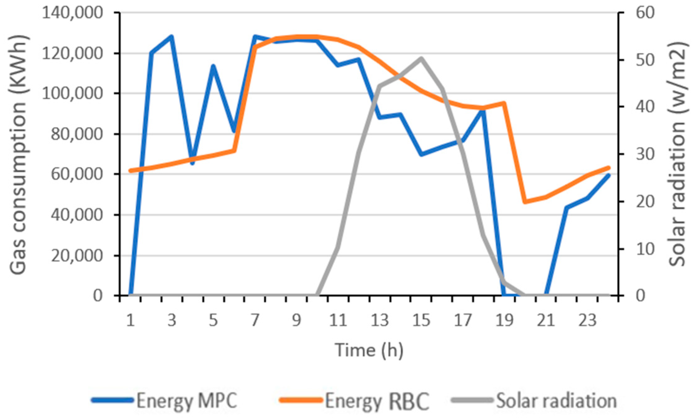Figure 17 compares the values of indoor temperature corresponding to the MPC against those of the RBC strategy over the 24 h timesteps of day 8. The reason behind the higher comfort score of the MPC is the decrease in temperatures during unoccupancy, as already explained. This cutdown of heating did not prohibit the strategy of restoring the comfort temperatures during occupation hours. Results show that in day 8, the MPC strategy consumed 11.6% less energy compared to the RBC strategy. This demonstrates that the proposed strategy was able to anticipate the expected solar radiation for the day and suggested heating setpoints that maintain comfort temperatures while minimizing energy consumption. Figure 18 compares the gas consumption of both strategies for day 8.

4. Discussion

In this paper, a predictive control strategy for a building’s heating system with radiators powered by a gas boiler was proposed aiming to balance thermal comfort and gas consumption. For this study, the occupant’s comfort was represented by the indoor air temperature, a common criterion in current building regulation systems. While future work may consider factors such as indoor air relative humidity, the study focused solely on temperature as the comfort indicator.

The proposed method relies on two prediction models informed by conventional building data, integrating weather and occupancy forecasts. The selection of these models was discussed in the paper, where several machine learning models were tested, and those demonstrating the highest prediction accuracy were chosen. The integration of historical data significantly improved precision. The neural network model aimed at predicting indoor temperature proved to be highly accurate, but the support vector machine model selected for predicting gas consumption, crucial for implementing the method, appears to have potential for improvement. The decision not to rely on internal measurements of technical equipment, such as various temperatures from the primary and secondary parts of the heating system, adds complexity to the modeling process. This aspect could be the focus of specific future research efforts. The two models, used to predict temperature and consumption over a 24 h forecasting horizon, are integrated within an optimization loop using genetic algorithms. The optimization phase aims to define an optimal sequence of setpoint temperatures for the secondary circuit’s water supply in the heating system on an hourly basis. The process of prediction and the calculation of the 24 h sequence of heating setpoint temperatures is repeated every hour, replacing the predicted values of indoor temperature and gas consumption at the next timestep, by the values simulated on the modeled building, preventing the accumulation of prediction errors throughout the horizon.

The method was developed using data generated in TRNSYS18. A case study building was modeled, and the simulation tool was employed to test and compare the predictive control strategy against a conventional Rule-Based Control strategy typically used in such buildings. It has been confirmed that the proposed MPC strategy can anticipate potential events (weather disturbances or internal gains) that could disrupt the building’s behavior, while achieving energy savings and maintaining occupant thermal comfort.

Because MPC strategies are implemented in buildings that vary in heating systems, environmental and weather conditions, and initial operating states, directly comparing their performance across studies is inherently challenging. Instead, comparison was performed against a reference model tailored to the same building, departing from the same initial conditions. By comparing our MPC-based strategy with an already optimized heating curve, we demonstrated additional energy savings, ranging between 3% and 30% across various randomly tested days. These results were obtained by combining a comfort score and a consumption score for each of these test days. A weighting between the two scores had to be chosen to achieve a compromise between thermal comfort and energy consumption. This weighting determines the balance of this compromise, and the choice of its value is left to the discretion of the operators, based on their priority for each part of the objective function.

This study shows that an MPC strategy can indeed be deployed with only a small set of readily obtained measurements, enabling straightforward transfer to other buildings with similar heating systems. Moving forward with the research, the goal is to implement the proposed control method on a real case study building. Measurements are currently being collected, and a predictive strategy is expected to be developed.