Abstract
As a key component of the power system, the good or bad conditions of synchronous machines will directly affect the stable supply of electric energy. The inter-turn short fault of the stator is one of the main dangers to the synchronous machine and is difficult to diagnose. Frequency response analysis has recently been introduced and used for detecting this type of fault; however, the fault degrees and locations cannot be directly recognized by traditional frequency response analysis. Therefore, this study improves the frequency response analysis by combining it with a deep learning model of a multivariate time series transformer. First, the principle of this study is introduced. Second, the frequency response data of short circuit faults are obtained using an artificially simulated experimental platform of a synchronous machine. The deep learning model is then well-trained. Finally, the performance of the proposed method is tested and verified. It concludes that the proposed method has the potential for classifying and diagnosing the inter-turn short circuit of stators in synchronous machines.
1. Introduction
A synchronous machine (SM) is a widely used device that converts mechanical energy to electricity; however, the synchronous machine may be affected by thermal, electromagnetic, and mechanical stresses during its operation, which can lead to failures. Common types of failures include gear and bearing failures, excitation system failures, stator failures, and rotor failures. Among them, stator failure is a typical failure with a high probability of occurrence. According to data statistics, it accounts for 38% of failures in medium-sized machines and 66% in large machines [1]. The stator faults mainly include inter-turn short circuit (ITSC) faults, insulation faults, and overheating faults, among which ITSC faults account for the highest proportion, reaching more than 50% of stator faults [2]. Therefore, ITSC faults are the main fault of SMs. It is necessary to quickly detect the stator ITSC fault; otherwise, if the machine continues to operate, the fault will develop and cause the machine to overheat and even shut down.
At present, there are some methods for detecting machine ITSC faults, including the direct current (DC) resistance method [3], the alternating current (AC) impedance test method [4], the repetitive surge oscilloscope (RSO) method [5], the open transformer method, and the detection coil method [6]. However, the DC resistance method is insensitive to ITSC faults. The detection effect of the AC impedance test method is affected by many factors like a rotor air gap, speed, impedance, etc., making it difficult to determine early ITSC faults. The RSO method cannot be used to locate the short circuit point. In the open transformer method, the rotor needs to be removed before conducting the experiment, which affects the operability of testing. The detection coil method requires an online application where the accuracy is affected by the armature reaction of the machine. Thus, researchers are still studying other methods to detect ITSC faults in synchronous machines.
Recently, frequency response analysis (FRA), a common method used to diagnose the winding deformation fault of a transformer, has been applied to fault diagnosis of rotating machinery [7,8]. FRA normally uses a sweep frequency signal to excite the tested object; thus, it is also called sweep frequency response analysis (SFRA). Reference [9] discussed the applicability of the SFRA for detecting inter-turn faults in machine stators, tested SFRA results under different degrees of ITSC faults, and proved that the SFRA method can be effectively used to detect inter-turn short circuit faults. Reference [10] introduced the application of the SFRA method in field winding fault detection in static excitation SMs. A large number of experiments were conducted on the on-site windings of SMs at static and different speeds. Reference [11] experimentally verified the relationship between the SFRA response and the rotor position of a salient pole machine and concluded that a reference rotor position for an SFRA diagnosis should be considered in the test. This study also verified that there is no need to remove the rotor when detecting the stator, making FRA technology more meaningful in field applications.
Although the SFRA has shown good potential for application, the interpretation of the FRA remains unsolved. The existence of ITSC faults can be diagnosed by comparing whether the SFRA curve has changed; however, the fault extents and locations cannot be directly diagnosed by the traditional SFRA method. Therefore, researchers are still working to address this issue. Reference [12] introduced statistical indicators for fault diagnosis using the FRA method. Due to the susceptibility of statistical indicators to measurement errors and external uncontrollable factors such as temperature and humidity, a trend curve method was further proposed to improve the accuracy of fault diagnosis. Yet, the fault location and specific fault extents cannot be detected by this method. Some studies also use machine learning technology to diagnose ITSC faults in machines [13,14]. For instance, reference [15] used a short-time Fourier transform of symmetrical components of a stator phase current to extract the signal of the single-turn short circuit in the stator of a permanent magnet synchronous machine and used machine learning algorithms such as support vector machine and naive Bayes to automatically detect and classify such faults. Reference [16] proposed a new method for offline inter-turn fault localization of synchronous machines based on frequency response and cascade machine learning technology. This method utilizes key information from the frequency response transfer function, combined with exponential Gaussian process regression and linear discriminant analysis, to estimate the short circuit faults.
From the above existing methods, it can be seen that there exist the following shortcomings:
(1) The statistical indicator-based fault diagnosis method cannot obtain detailed information about fault degrees and locations, which is because there is no direct and obvious relationship between fault degrees/locations and statistical indicators. In addition, the used indicator threshold is derived from small sample data, which is not objective enough and easily influenced by statistical error and external factors.
(2) Although the traditional machine learning-based diagnosis method can achieve fault diagnosis, it cannot self-update or learn. Additionally, artificial feature engineering is frequently and highly needed, and different feature engineering would have a significant impact on the performance of the diagnosis model. Furthermore, the machine learning-based method has poor generalization.
Recently, deep learning techniques have developed rapidly, achieving remarkable results in fields such as computer vision, natural language processing, and others. Deep learning has also been used to diagnose short-circuit faults in electrical machinery. Many studies use conventional convolutional neural networks (CNNs), transfer learning, or variations of those models to identify the online condition of a permanent magnet synchronous motor (PMSM). Reference [17] constructed a synchronized dataset of current and vibration signals and presented a multi-source data-fusion algorithm based on CNNs to derive an early-stage ITSC fault-severity indicator of a PMSM. Reference [18] used the stray flux and current of a PMSM to detect low-severity ITSC faults. The study presents a classification of multiple faults at low severity levels under variable speed conditions using a transfer learning-based approach with pre-trained models. Reference [19] developed a PMSM fault detection system based on direct processing of phase-current signals using a CNN and transfer learning. It experimentally verified the diagnostic systems developed in steady and transient states during changes in load torque and speed. Reference [20] collected current and vibration signals of a PMSM and transformed them into statistical features. Various operating faults were diagnosed utilizing an improved CNN, namely, a deep-regulated neural network (RegNet). Reference [21] used the current signal of a PMSM to classify fault levels of minor ITSC faults. It adopts support vector machines (SVMs) and CNNs to train the diagnosis model with experimental data collected from tests in the laboratory. From the above literature review, most studies use flux, current, vibration signals, and deep learning to characterize the status of a PMSM; however, they did not focus on the synchronous generator. Additionally, there are few reports on the use of deep learning techniques for processing the SFRA curves of the generator; namely, an alternative wide frequency electrical characteristic curve could also contain fault information for SMs.
Based on the above situations, an improved method is introduced for intelligent diagnosis of SMs in this study. The innovations and advantages of the proposed method are as follows:
(1) A new diagnostic method of stator ITSC faults in SMs based on SFRA and a Multivariate Time Series Transformer (MTST) is proposed and studied. Deep learning architecture is used to process the SFRA curves of the SM.
(2) Both ITSC fault extents and locations of stator winding can be distinguished. By constructing a multi-level neural network to automatically extract the features of SFRA curves, it has stronger representation and generalization capabilities, which also have low demand for feature engineering.
The rest of the paper is organized as follows: Section 2 shows the basic principles of SFRA and MTST. The experimental platform of the SM and the ITSC simulation experiments are introduced in Section 3, while the diagnosis of stator ITSC faults in SMs is presented in Section 4. Section 5 introduces the conclusion.
2. Basic Principles of SFRA and MTST
2.1. Introduction to SFRA
Traditionally, the SFRA method is commonly used for winding deformation fault diagnosis of power transformers. Due to the many similarities between transformer windings and machine windings, the SFRA method has gradually been applied to fault detection in machines. The basic unit of the equivalent circuit of the machine stator at high frequency can be represented as an RLC circuit composed of resistors, inductors, and capacitors in series and parallel.
A series of sine signals (1 Hz~1 MHz) with the same amplitude but different frequencies are injected into the first terminal of the SM stator, and the SFRA curve of the SM is obtained by measuring the excitation voltage at the first terminal and the response voltage at the end terminal of the stator.
where is the response voltage at the end terminal, is the excitation voltage at the first terminal, is the SFRA response of the winding, is the amplitude-frequency response, and is the phase-frequency response.
To detect SM faults, a healthy SFRA test should be measured as a reference. When the SM experiences an ITSC fault, the internal circuit parameters will inevitably change, and the obtained SFRA curve will also change accordingly. By comparing the SFRA curve of the winding in the fault state with those in the healthy state, the winding state can be analyzed to detect winding faults [7,11,13]. Furthermore, because the SFRA can be applied during regular inspections of synchronous machines (SMs), the real-time performance of diagnosis is not a major factor to consider.
2.2. Introduction to the Structure of MTST
An SFRA curve can be regarded as both sequence data and image data; however, if the SFRA curve is regarded as image data, there will be a large number of blank areas in the FRA image, which results in a sparse data matrix input. It is difficult to process such data structures from the perspective of the image. Thus, in this study, we treat SFRA curves as sequence data. The transformer architecture-based model is quite suitable for processing sequence data. It can effectively capture the complex relationships between different positions in a sequence through its unique self-attention mechanism and multi-layer structure. Therefore, this article uses the MTST model based on the original Transformer model for diagnosing stator ITSC faults in SMs. The model includes four sub-modules: data preprocessing, position encoding and linear mapping addition, Transformer encoder architecture, and output layer.
(1) Data preprocessing: Firstly, the SFRA data of the SM winding are preprocessed, which can enhance the universality of the model. The input features of each sample are obtained with a size of (1000,2). Each row of features represents the frequency, and each column represents a different SFRA amplitude-frequency characteristic curve. The calculation formula is shown in Equation (4).
where feature1 is the input feature matrix of the sample, TFtest is the SFRA amplitude-frequency characteristic curve of the tested winding (dimension: 1000 × 1), and TFnormal is the SFRA amplitude-frequency characteristic curve of the healthy winding (dimension: 1000 × 1).
(2) Addition of position encoding and linear mapping: After the data are preprocessed, each feature vector is normalized and then linearly mapped into a vector space with a dimension of 64, resulting in Ut. The calculation formula is shown in Equation (5).
where Ut is the word vectors in the original Transformer model, and Wp and bp are the learnable parameters of the model.
When using the MTST model for fault diagnosis of an SM, the position encoding in the original Transformer structure is selected and added to the input vector. The calculation formula is shown in Equation (6).
where U’ is the input of the Encoder and Wpos is the position encoding.
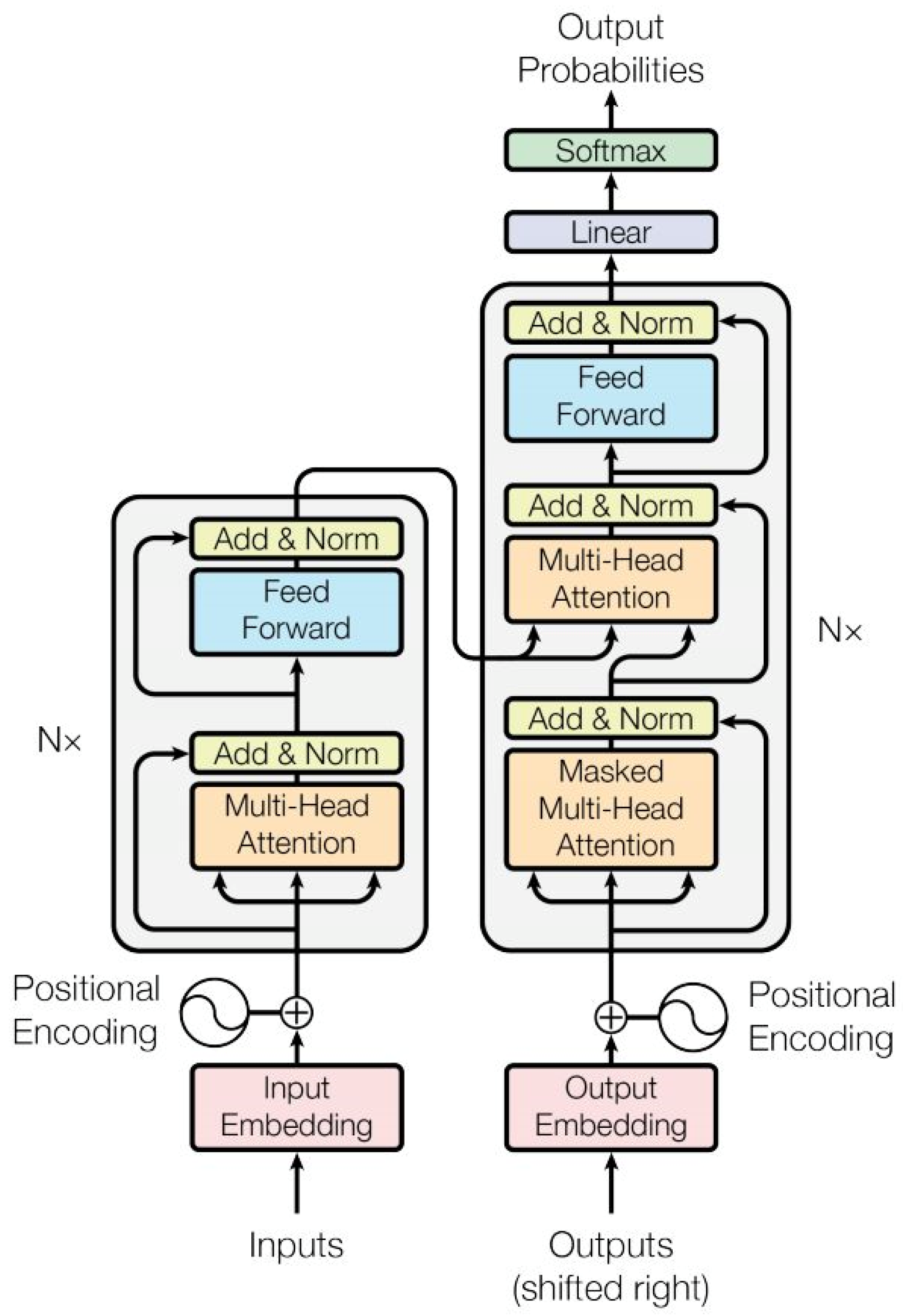
(3) Transformer Encoder structure: This diagnosis model consists of a Transformer Encoder structure. The Transformer model is mainly divided into two parts: the Encoder and the Decoder. The overall architecture of the model is shown in Figure 1.
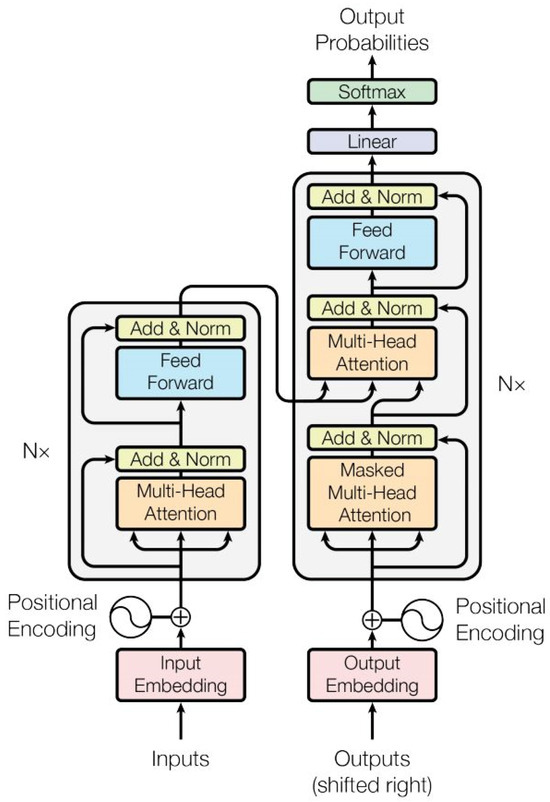
Figure 1.
Architecture of the Transformer model [22].
The function of an Encoder is to extract features from input data, also known as encoding. The Encoder is composed of multiple stacked encoder layers. As mentioned before, MTST first performs vector encoding on the input sequence. As the framework processes data in parallel, position encoding is required to record the sensitive positional relationships of each element in the sequence. Next, the position encoding is added to the input vector to form a vector with positional information, which is input into the Transformer Encoder. In the Encoder structure, the following steps are performed: multi-head attention mechanism, residual connection, normalization, feedforward neural network, residual connection, and normalization.
This proposed MTST model is composed of three stacked Encoder layers. The specific configuration of a single Transformer Encoder structure is as follows:
Multi-head attention mechanism: By placing U′ in different single-head self-attention mechanisms, output results are obtained in eight spaces.
Residual connection, normalization, and feedforward neural networks: In this article, the structure of residual connections, normalization, and location-based feedforward neural networks is consistent with the original Transformer model.
(4) Output layer: After being processed by three Encoders, Z is the output, and Z is then input into the linear layer for calculation. Finally, the softmax function is used to convert the output of the linear layer into the probability distribution of the corresponding class of the sample. In this study, there are a total of 10 types of ITSC faults for classification, which will also be introduced in detail in Section 4.
3. The Artificially Simulated ITSC Fault Experiments
3.1. Introduction to the Experimental Platform of the SM
This article takes a fault simulation salient pole SM in the laboratory as the analysis object. The generator is coaxially connected to a driving motor, which simulates the prime motor. The speed of the driving motor and the excitation part of the SM are adjustable. The main technical parameters are shown in Table 1.

Table 1.
Basic parameters of the synchronous machine.
The A-phase stator of this SM is equipped with 16 terminal points at the beginning, middle, and end of the winding, as well as four terminal points for the B-phase and four terminal points for the C-phase. It can simulate ITSC faults in the stator at different short-circuit positions and degrees by simplifying the short-circuiting of the corresponding terminal points.
In the experiment, to obtain comprehensive and accurate SFRA data of the ITSC fault of the SM, the terminal taps of phase A of the SM stator were selected for the experiment. Different resistance values were connected in series between two short-circuit taps to simulate different degrees of ITSC faults. The stator ITSC faults at different positions were achieved by short-circuiting the taps at different terminal taps of the SM.
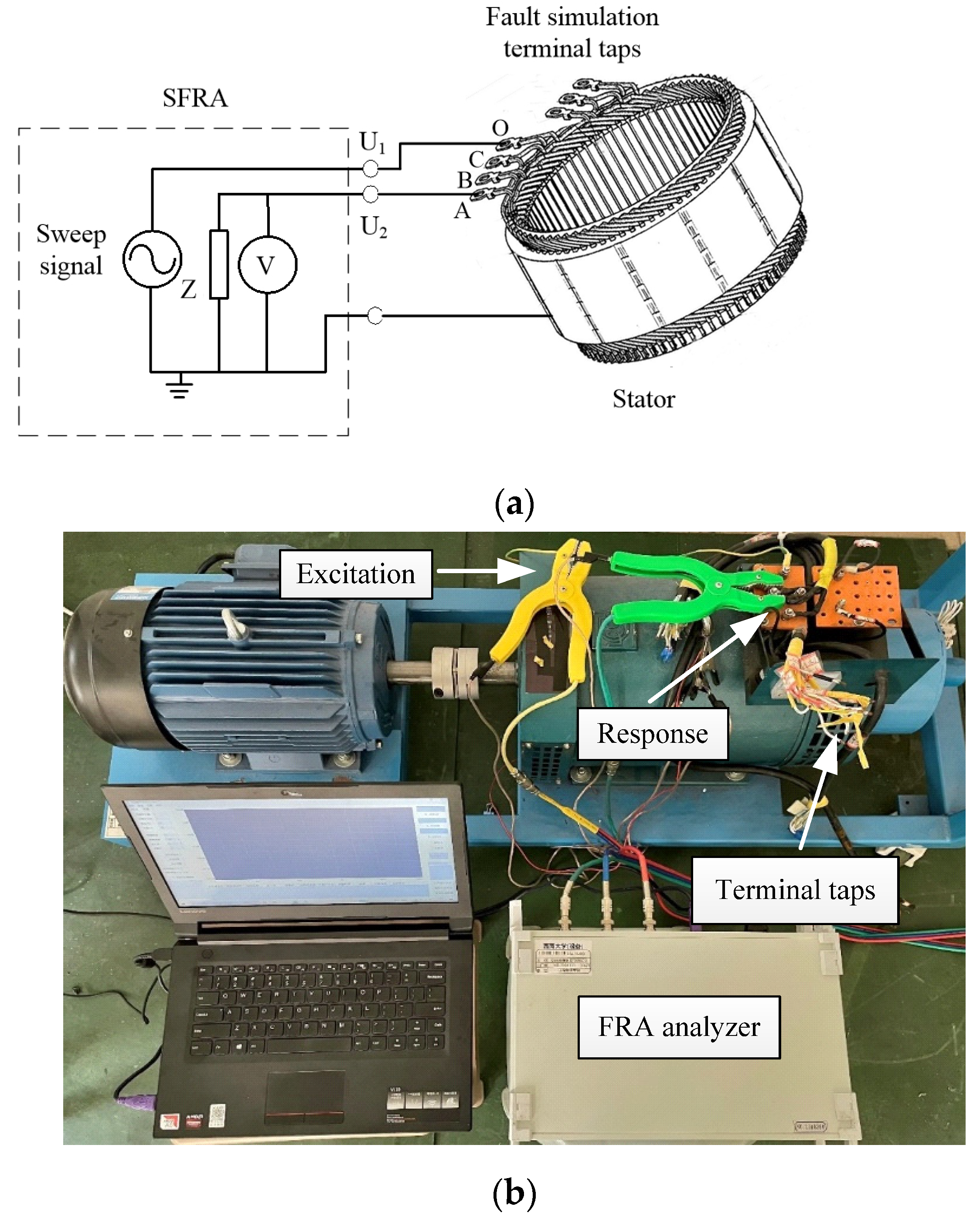
An FRA analyzer in the laboratory was used for testing. The wiring of the artificially simulated fault experiment and the overall appearance diagram are shown in Figure 2. Due to the basic principle of the FRA experiment and set requirements of the FRA analyzer, the measured impedance is set to 50 Ω to match the impedance of the connecting coaxial cable, the sweep frequency range is set to 1–1000 kHz, the sweep frequency interval is set to 1 kHz to capture more details about small resonances, and the number of sweep frequency points is 1000. Additionally, it has already been demonstrated that ITSC faults have a significant impact on the SFRA curve between 1 Hz and 1 MHz, especially the characteristic frequency bands and resonances between several kHz and several hundred kHz [9,10,11,12]. The above experimental setup is feasible.
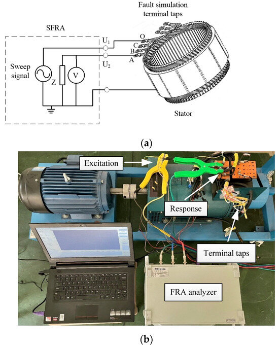
Figure 2.
Connection diagram for simulating ITSC faults in the SM in an experiment: (a) SFRA test diagram of the stator in the SM; (b) field connection diagram.
In addition, before the ITSC fault simulation experiment, we studied the impact of rotor position on the SFRA curves of the stator. The rotor is varied for different angles. The angle is defined as the degree of angle between one pole of the rotor and one slot of the stator, as shown in Figure 3a. The SFRA test results are shown in Figure 3b. It is found that the rotor position has a significant impact on the SFRA curve of the stator, especially in the resonance points and gains of low- and medium-frequency bands. This is because the different positions of the rotor can change the equivalent circuit parameters of the stator winding, especially the inductance, leading to changes in the SFRA curve. At high frequencies (>800 kHz), the infiltration of magnetic flux into the iron core might be ignored, and the influence of rotor position is negligible. Therefore, the SFRA curve remains basically unchanged. It is also found that when the rotor position is at 0° and 90°, as well as 45° and 135°, the SFRA curves are the same. This is because the salient pole SM has a geometrically symmetrical structure. In the following artificially simulated ITSC fault experiment, it is obvious that the rotor position should be marked and fixed when the SFRA test of the stator is performed. If the SFRA test is performed when the SM is not at service status, the rotor excitation should be OFF.
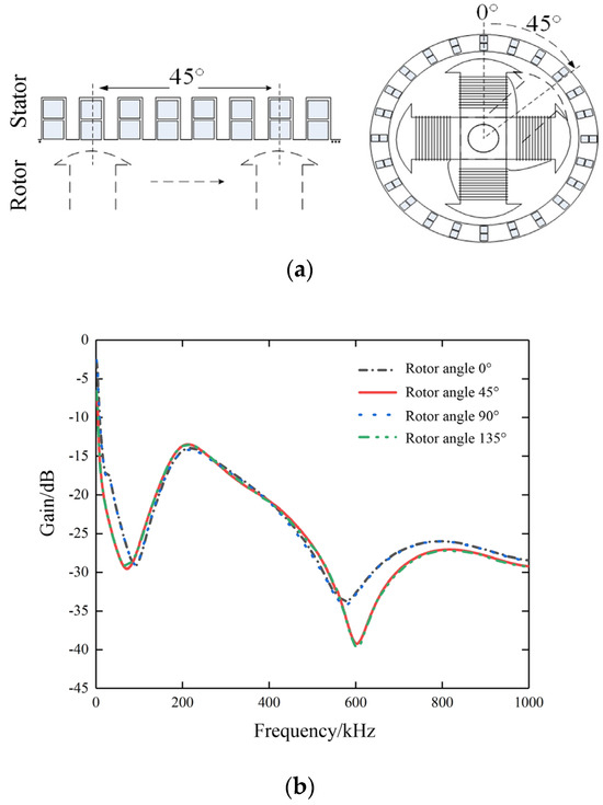
Figure 3.
Impact of rotor position on the SFRA curve of the stator: (a) schematic diagram of the rotor rotation for the salient pole SM; (b) SFRA curves of the stator under different rotor statuses.
3.2. The Experimental Result of Artificially Simulated ITSC Faults in the SM
Based on the above experiment platform, we first conducted a reference experiment to obtain the SFRA curve of the SM in a healthy state. Then, we performed the artificially simulated ITSC fault with different fault extents and locations. At the head, middle, and end locations of the stator, a total of six terminal taps are led out, X1~X6, representing the six different positions of the stator winding. Each terminal leads out a tap, representing ten turns in the slot of the SM. Two taps of terminal X1 are connected to make it short-circuited with one turn, and it is connected with four different resistance values of 0.5 Ω, 2.5 Ω, 5 Ω, and 10 Ω in series between the taps to simulate different degrees of ITSC faults. Among them, 5 Ω and 10 Ω represent the slight degree of ITSC faults, 0.5 Ω and 2.5 Ω represent the moderate degree of ITSC faults in the SM, and 0 Ω represents a direct short circuit, which is the most serious degree of fault. The fault setting method for other terminal taps of the stator winding is the same as that for terminal X1.
The fault setup of the ITSC fault and the values of the added resistance are based on References [10,11,23]. Reference [10] added resistors of 0.2 Ω, 1 Ω, 10 Ω, and 100 Ω between fault taps X1–X2 of the machine and compared the obtained SFRA curves. The results showed that the resistance values had an impact on the low-frequency range of the SFRA curve, and the SFRA method could detect inter-turn short circuit faults with different resistance values. Reference [11] used 2–10 Ω resistance values for SM simulating inter-turn short circuit fault detection to verify whether the FRA method can detect ITSC faults with different degrees. Reference [23] selected fault resistors of 0 and 5 Ω and conducted a large number of ground fault and ITSC fault experiments on hydroelectric generators, verifying the effectiveness of the proposed diagnostic method. The above references all added different resistance values for testing SM turn-to-turn short circuit faults, and the values were less than 10 Ω. Therefore, this study refers to the above experiment and sets four different resistance values of 0.5 Ω, 2.5 Ω, 5 Ω, and 10 Ω to simulate different degrees of ITSC faults.
Finally, the ITSC faults in stator windings of the SM with different fault locations and extents are tested. A total of 50 sets of repeated experiments were conducted for each fault, and a total of 1500 sets of experimental data were obtained. The specific ITSC fault-setting scheme is shown in Table 2.
Table 2.
Experiment setup of ITSC fault on a 7.5 kW SM.
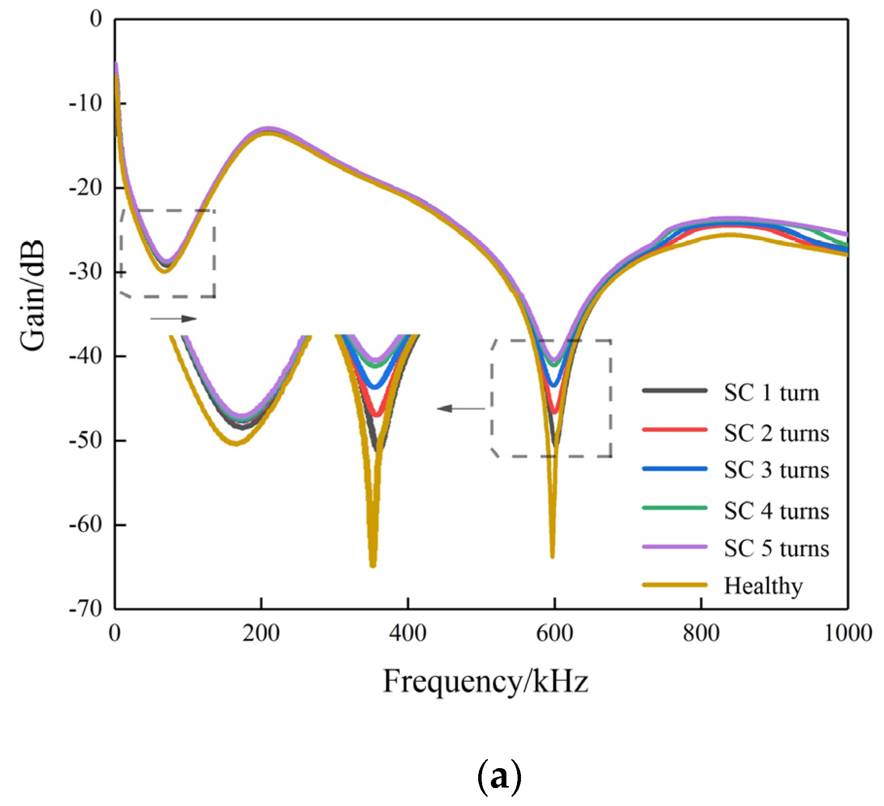
Taking the X1 terminal tap of the stator A-phase of the SM as an example, the SFRA curves under healthy conditions and different degrees of ITSC faults are shown in Figure 4. From Figure 4, it can be seen that when the ITSC fault extent is different, the SFRA curve of the SM does not coincide with the curve of the normal winding, and there are varying degrees of deviation in the low, medium, and high-frequency ranges, with the maximum deviation observed in the low and medium frequency ranges.
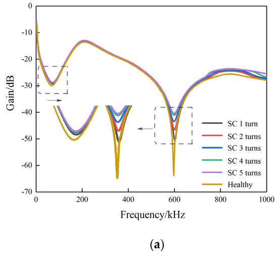

Figure 4.
SFRA curves of the SM under different degrees of ITSC faults: (a) short circuit with different turns; (b) short circuit with different resistances.
As shown in Figure 4a,b, as the number of short circuit turns increases and the short circuit resistance decreases, the degree of ITSC fault increases, and the resonant point of the SFRA curve shifts to the high frequency as a whole. Meanwhile, the gain also increases with the degree of fault. Therefore, as the degree of fault increases, the deviation trend of the curve is similar. The SFRA curve deviation can be explained as follows:
First, when an ITSC fault occurs in the stator winding, the inductance parameter is mainly changed, resulting in the deviation of the SFRA curves in low and medium frequency bands. As the degree of stator ITSC fault increases, the effective number of stator turns decreases, and the inductance of the winding gradually decreases. However, the capacitance value did not have significant variations because the dielectric material and distance only changed a little. Thus, according to Equation (7), the resonant point frequency of the curve increases.
where L is the inductance of winding, C is the capacitance of winding, and f is the resonant frequency.
Second, according to the equivalent circuit of the SFRA analyzer connecting with the winding, the equivalent resistance of the measuring cable (50 Ω) and winding equivalent impedance are connected in series, and the response voltage of the FRA instrument shares a portion of the excitation sweep voltage. Therefore, with the increasing ITSC fault degree, the inductance value of the stator winding is decreased, the impedance of the stator decreases, and, at the resonant point, the gain of the SFRA curves increases.
Additionally, because the SFRA is measured in the offline status of the SM and only the one-phase stator is energized, we do not need to consider the phase balance, sequence components, and three-phase operation of the SM. However, for fault propagation, it is possible that the non-tested phase fault could have an impact on the FRA curve of the tested winding. We studied the impact of the non-tested phase inter-turn short circuit fault and grounded fault on the frequency response curve of the tested phase stator and found that the impact is significant; however, the variation patterns of these FRA curves are quite different from that of the stator phase with an ITSC fault. The above phenomena are consistent with those described in References [10,24]. Therefore, the ITSC fault of the stator can be distinguished.
Additionally, SFRA experiments were conducted under different internal winding faults and external environments. Statistical evaluation is necessary to ensure the significance and reliability of experimental data. We have also, accordingly, performed the hypothesis testing of SFRA data using the chi-square test. The SFRA data are 1500 × 1000, in which 1500 represents FRA samples of different simulated faults, while 1000 represents the features of the FRA curve. We also performed a goodness-of-fit test and an independence test. It is found that the chi-square statistic is 54,482, the degree of freedom is 72, the p-value is around zero, and the conclusion is as follows: rejecting the null hypothesis, there are significant differences in the distribution of data for different types of simulated faults, which demonstrates the reliability of the experiments.
4. Diagnosis of Stator ITSC Faults in SMs Based on MTST
4.1. Flowchart of Fault Diagnosis
The diagnosis method for ITSC faults in SM stator windings based on MTST mainly includes the following stages, as shown in the flowchart in Figure 5.
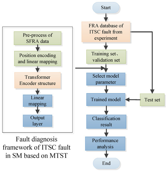
Figure 5.
Flowchart of the MTST-based diagnosis method for the SM.
(1) Firstly, the raw SFRA data obtained from the experiment are preprocessed to obtain the feature vectors;
(2) The position encoding and linear mapping are then added to process the feature vectors;
(3) The result obtained in (2) is input into the encoder architecture of the MTST model, and the output result is obtained after linear mapping, which includes classification information;
(4) The MTST-based fault diagnosis model is trained, and its performance is evaluated;
(5) The database is divided into a training set, validation set, and testing set, and the training set and validation set are used to select the adjustable parameters of the model. The optimal parameters are then obtained, and the trained diagnostic model is obtained. Finally, the trained model is tested using the test set, which outputs the classification results, and the classification results are evaluated.
4.2. Setup of the Fault Diagnosis Model
Based on the experimental result of the ITSC fault in Section 3, the stator winding faults are classified into 10 categories according to fault location and severity. They include slight ITSC fault, moderate ITSC fault, and severe ITSC fault at the head position of the stator; minor ITSC fault, moderate ITSC fault, and severe ITSC fault in the middle position of the stator; minor ITSC fault, moderate ITSC fault, and severe ITSC fault at the end position of the stator; and healthy status, as shown in Table 3.
Table 3.
Classification labels of fault degree and location.
The configuration of the server during the training of the designed model programming implementation is shown as follows: the CPU is Inter(R) Xeon(R) Gold 6268CL×2 (INTEL CORP., Hillsboro, USA), the GPU is NVIDIA RTX A4000 (NVIDIA CORP., California, USA), the RAM is 128G(SAMSUNG CORP., Suwon, Korea), and PyTorch 2.5.1, NumPy 2.1.3, and Tsai 0.4.0 are used. The training parameters of the MTST model are as follows: the learning rate is set to 1 × 10⁻⁴, the batch size is set to 32, the proportion of the training set is 70%, and both proportions of the testing set and validation set are 15%. The parameter settings for the model architecture are shown as follows: the number of encoder modules is 3, the number of heads is 8, the dim.model is 64, and batch normalization is used. The encoder part of a complete Transformer model typically consists of six encoder layers; however, to reduce computations, small experimental models may use fewer, 2–4 layers; thus, we chose three encoder layers. The rest of the parameters are unchanged. As shown below, it is feasible to use these parameters to achieve satisfactory prediction results.
Because the deep learning model has to be well-trained before its real application, the training time of the model is not a major factor. Yet, thousands of samples are used to train the model, and the training time of a new model is about several tens of hours. Moreover, it is possible to use the transfer learning technique to accelerate the training process so the training time can be reduced to several hours.
4.3. Result of Fault Diagnosis
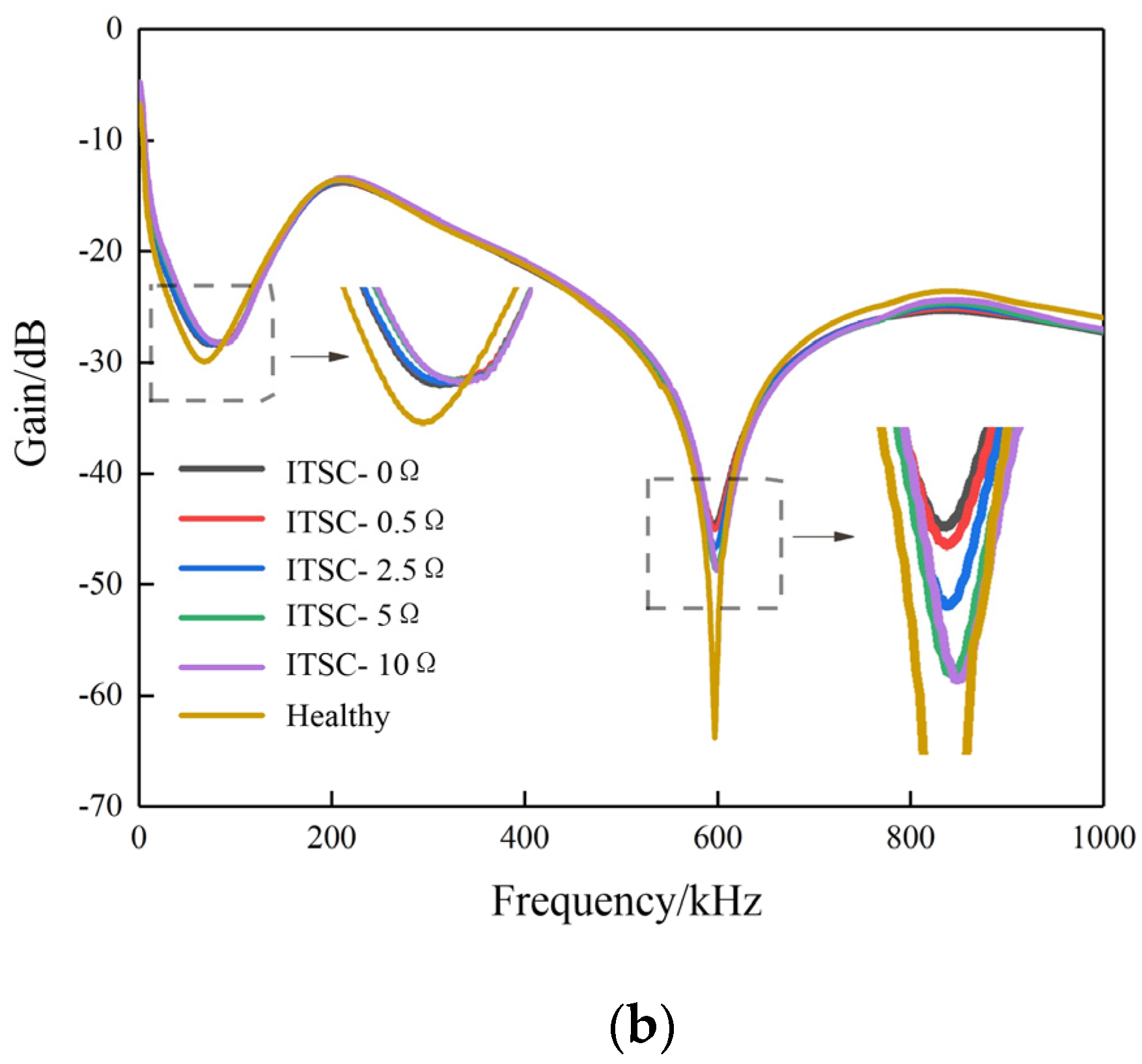
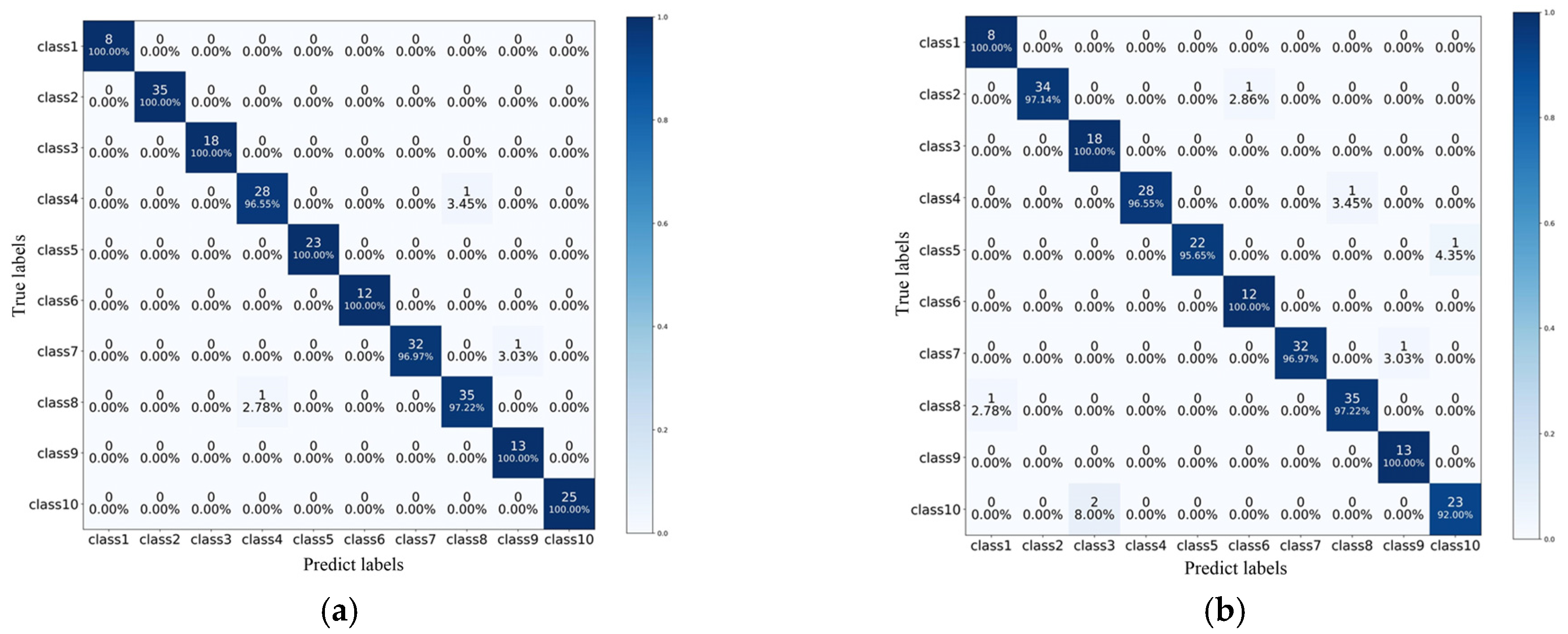
The model with the final parameters is saved, and the iteration is set and limited to 500 times. The loss function curve on the training set and validation set during the model training process and the confusion matrix are shown in Figure 6.
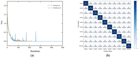
Figure 6.
Loss curve and confusion matrix during the training process: (a) loss curve; (b) confusion matrix.
From the above figure, it can be seen that the overall performance of the MTST model improves during the training process, with slight fluctuations, and then tends to stabilize. Figure 6a concludes that the loss of the model does not increase with the increase in iterations, indicating that the model does not overfit and performs roughly the same on the training and validation sets. The MTST model converges to a good performance after 100 iterations, and the final recognition accuracy of the model in the training and validation sets is 99.57%. The confusion matrix output by this model is shown in Figure 6b, and the class labels have already been defined in Table 3, which is a combination of fault locations and degrees. It can be seen that only one sample of class 8, namely, the moderate fault at the end of the winding, was misclassified as class 3. The diagnostic error in this case is calculated as 0.43%.
Additionally, we performed a 5-fold cross-validation to verify the model’s generalization ability. The Transformer model has several parameters, and the computational cost of training 1000-length sequences is relatively high. The 5-fold cross-validation is more efficient than the 10-fold cross-validation. The results are as follows: the mean accuracy is 99.17% ± 0.0018, and the average macro F1 is 98.88%. The results show that the performance of the model is stable across different training validation set partitions, and the model has a strong predictive ability and good generalization performance on the entire dataset.
From the above results, it can be seen that the MTST model using a Transformer structure performs strongly in both the training and validation sets and can distinguish ten types of faults with high classification accuracy. Therefore, the MTST method has a strong learning ability in the diagnosis of stator ITSC faults in this SM. Furthermore, since the interpretability of the deep learning model can be analyzed to study the internal working mechanism of the diagnosis process, we have studied the interpretability based on frequency response and a feature importance analysis method, namely, the smooth grade and gradient-based class activation maps (Smooth Grad-CAM++) [25]. It is found that the deep learning model pays much attention to the resonant point variations and the difference between healthy and normal FRA curves, which is similar to the human judgment process and the working mechanism of the diagnosis model.
4.4. Comparison with Other Sequence-Based Models
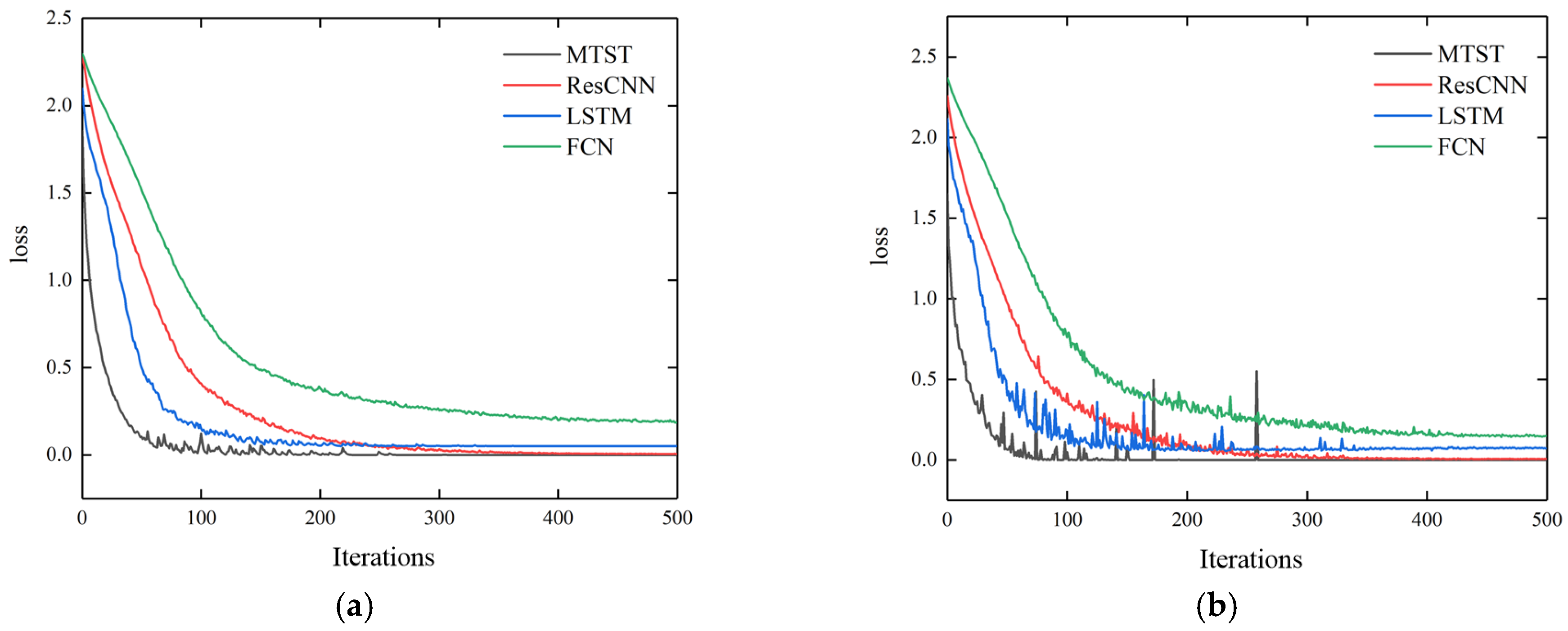
Some other common fault diagnosis architectures, mainly the sequence-based models, are also studied and compared, including Residual Convolutional Neural Network (ResCNN), Fully Convolutional Neural Network (FCN), Long Short-Term Memory (LSTM), and Random Forest (RF). Among these, both ResCNN and FCN are variations in convolutional neural network (CNN) architecture, in which ResCNN adds residual connections in the CNN architecture to relieve the vanishing gradient problem in deep neural networks. LSTM is also common for processing sequence data because of its nature. RF is a common machine learning algorithm. The same fault dataset is input into the above models to obtain fault classification results, which are compared with those of the MTST method. The accuracy curves of each model for the validation set during the training process are shown in Figure 7. The loss function curves for the training and validation sets are shown in Figure 8.
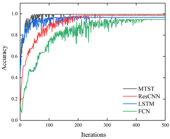
Figure 7.
Accuracy of MTST and other common models in the training process.
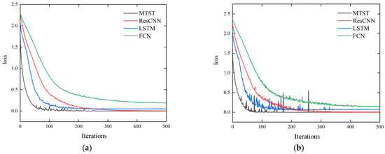
Figure 8.
Loss curves of MTST and other models during training: (a) loss curve for the training set; (b) loss curve for the validation set.
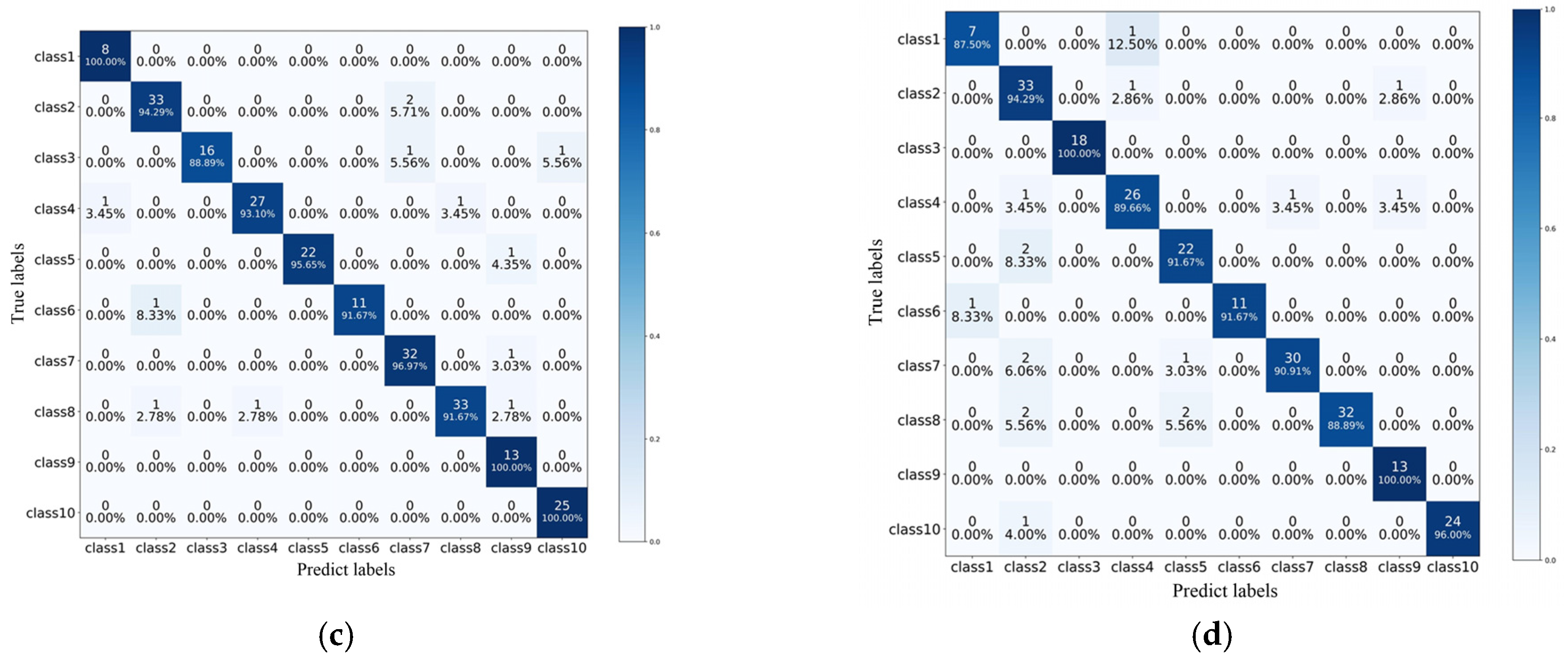
The confusion matrix of MTST and other models for the validation set is shown in Figure 9. For simplicity, the mean accuracy comparison between MTST and other models is shown in Table 4. From Table 4 and Figure 7, Figure 8 and Figure 9, it can be seen that the fault diagnosis accuracy of MTST is 99.57%, ResCNN is 98.71%, FCN is 94.83%, LSTM is 96.98%, and Random Forest is 92.67%.
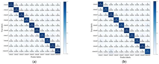
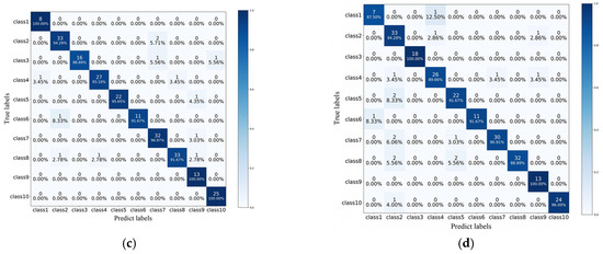
Figure 9.
Confusion matrix of MTST with other models for the validation set: (a) ResCNN; (b) LSTM; (c) FCN; (d) RF.
Table 4.
Comparison of this study with other models on a 7.5 kW SM.
The MTST algorithm can perform parallel computing, making the calculation process faster, and MTST has a multi-head attention mechanism. During the calculation process, sequences with longer signals can still focus on effective information through their unique mechanism. The implementation of parallel computing for ResCNN, FCN, LSTM, and RF algorithms is relatively complex, and the RF algorithm is a traditional intelligent algorithm that requires specific formulas to extract features from parameters. It does not have learnable parameters, and its constant feature extraction method limits its upper-performance limit. Thus, the MTST model used in this paper has the best classification performance compared to the other four methods.
4.5. Performance of the Proposed Method on Different SMs
To further verify the performance of the proposed method in the diagnosis of ITSC faults in SMs, this paper conducted stator fault experiments on another 5 kW SM in the laboratory. The parameters of the SM are shown. The rated power is 5 kW, the rated voltage is 380 V, the pole pair is 1, the slot of the stator is 36, and the rated speed is 1500 r/min.
The fault setting for the experiment is the same as that of Section 3.2. Due to the fact that there are only three terminals to simulate the ITSC faults, named X1, X2, and X3, respectively, different resistors of 0–10 Ω were used, with terminals X1–X2 and X2–X3 to simulate faults at different locations and degrees. The experiment setup of the ITSC fault is shown in Table 5, and the image of the fault experiment is shown in Figure 10.
Table 5.
Experiment setup of an ITSC fault on a 5 kW SM.
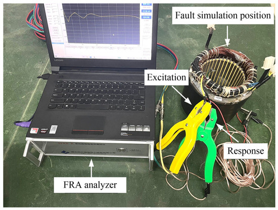
Figure 10.
Image of the fault experiment on another 5 kW SM.
A total of 500 sets of experimental SFRA data of ITSC faults in the stator of the SM were obtained. Similar to the signal processing mentioned earlier, these data were input into MTST, ResCNN, FCN, LSTM, and RF models. The mean accuracy of the fault diagnosis of these models is 99.05%, 98.10%, 96.19%, 95.24%, and 93.33%, respectively.
According to the experimental results, the fault diagnosis accuracies of the ResCNN, FCN, LSTM, and RF models are 98.10%, 96.19%, 95.24%, and 93.33%, respectively; all are lower than the 99.05% of the MTST model. The above results once again verify that the proposed diagnosis method has better classification performance than other methods and has good generalization.
In addition, compared to the original Transformer model, the computational complexity of the proposed model is significantly decreased. Some dedicated NPUs or FPGA acceleration with enough RAM can be used to load the proposed deep learning model, and if quantification, pruning, or distillation techniques are used, the MCU or edge AI chip with a smaller RAM can also be used, making it possible to be easily used for industrial applications.
5. Conclusions
A new method that facilitates the diagnosis of stator inter-turn short circuit faults in synchronous machines was introduced. It combines the SFRA and MTST methods for classifying the faults. The proposed method improves the existing SFRA by potentially diagnosing the fault degree and locations of stator ITSC faults. The following conclusions can be derived:
(1) An experimental platform of the SM that can artificially simulate an ITSC fault was established, a number of ITSC faults with diverse fault degrees and locations were simulated, and the corresponding SFRA data were measured.
(2) The experiment found that the SFRA curves of the faulty winding did not coincide with the curve of the normal winding, and there were varying degrees of deviation in the low, medium, and high-frequency ranges. Among them, the curve of the low and medium frequency ranges had the largest deviation. As the degree of ITSC fault increased, the resonance points of the SFRA curve shifted to a high frequency relative to those of the healthy curve, and the gain gradually increased. The SFRA data obtained from the experiment provide a basis for the diagnosis of ITSC faults.
(3) In the diagnosis of ITSC faults in the SM stator winding, the accuracy of the MTST algorithm diagnosis reaches 99.57%. Its accuracy is higher than those of the ResCNN, FCN, LSTM, and RF algorithms, which are 98.71%, 94.83%, 96.98%, and 92.67%, respectively. Other indicators also indicate that the proposed MTST-based method has better performance. Most importantly, both degrees and locations of ITSC faults can be identified using SFRA and the proposed model.
(4) Although the proposed method shows good performance, there are still some shortcomings. For instance, due to a lack of experimental conditions, the generalization of the technique has not been demonstrated by various SMs with different structures and parameters. The problem of fault propagation should also be discussed and verified by several experiments in the next step. After accumulating a large number of long-term cases, transfer learning may also be used for optimizing the proposed model to adapt to different SMs by adjusting the parameters of the last several layers. Furthermore, the robustness and noise resistance of the method should also be improved to be suitable for different noisy signals. The above shortcomings will be studied in the next step.
Author Contributions
Conceptualization, J.D.; methodology, Z.Z.; software, J.D.; validation, J.D. and Z.Z.; formal analysis, J.D.; investigation, Z.Z.; resources, J.D.; data curation, J.D.; writing—original draft preparation, J.D.; writing—review and editing, Z.Z.; visualization, J.D.; supervision, Z.Z.; project administration, Z.Z.; funding acquisition, Z.Z. All authors have read and agreed to the published version of the manuscript.
Funding
This research was funded by the Sichuan Science and Technology Program, grant number 2023 NSFSC0829; National Natural Science Foundation of China, grant number 51807166.
Data Availability Statement
The raw data supporting the conclusions of this article will be made available by the authors upon request.
Conflicts of Interest
The authors declare no conflicts of interest.
Abbreviations
The following abbreviations are used in this manuscript:
| SM | Synchronous Machine |
| ITSC | Inter-Turn Short Circuit |
| DC | Direct Current |
| AC | Alternating Current |
| RSO | Repetitive Surge Oscilloscope |
| FRA | Frequency Response Analysis |
| SFRA | Sweep Frequency Response Analysis |
| CNN | Convolutional Neural Network |
| PMSM | Permanent Magnet Synchronous Motor |
| RegNet | Deep Regulated Neural Network |
| MTST | Multivariate Time Series Transformer |
| ResCNN | Residual Convolutional Neural Network |
| FCN | Fully Convolutional Neural Network |
| LSTM | Long Short-Term Memory |
| RF | Random Forest |
References
- Yu, Y.Q.; Zhao, Z.Y.; Chen, Y.; Wu, H.; Tang, C.; Gu, W. Evaluation of the Applicability of IFRA for Short Circuit Fault Detection of Stator Windings in Synchronous Machines. IEEE Trans. Instrum. Meas. 2022, 71, 1–12. [Google Scholar] [CrossRef]
- Sergakis, A.; Salinas, M.; Gkiolekas, N.; Gyftakis, K.N. A Review of Condition Monitoring of Permanent Magnet Synchronous Machines: Techniques, Challenges and Future Directions. Energies 2025, 18, 1177. [Google Scholar] [CrossRef]
- Rafiei, V.; Khoshlessan, M.; Narvaez, C.C.; Fahimi, B. Detection of Inter-Turn Short Circuit in Stator Windings of Electric Machines Using Magnetic Symmetry Index and Machine Learning Methods. IEEE Trans. Energy Convers. 2025, 40, 642–652. [Google Scholar] [CrossRef]
- Ruiz-Sarrio, J.E.; Antonino-Daviu, J.A.; Navarro-Navarro, A.; Biot-Monterde, V. A Review of Broadband Frequency Techniques for Insulation Monitoring and Diagnosis in Rotating Electrical Machines. IEEE Trans. Ind. Appl. 2024, 60, 6092–6102. [Google Scholar] [CrossRef]
- Froehlich, P.; Oettl, F.; Lachance, M. Rotor Winding Diagnosis Using Sweep Frequency Response Analysis and Comparison to RSO. In Proceedings of the 2024 IEEE Electrical Insulation Conference (EIC), Minneapolis, MN, USA, 2–6 June 2024; pp. 333–338. [Google Scholar]
- Niu, G.; Dong, X.; Chen, Y.J. Motor Fault Diagnostics Based on Current Signatures: A Review. IEEE Trans. Instrum. Meas. 2023, 72, 3520919. [Google Scholar] [CrossRef]
- Zhao, Z.Y.; Chen, Y.; Yu, Y.Q.; Han, M.; Tang, C.; Yao, C. Equivalent Broadband Electrical Circuit of Synchronous Machine Winding for Frequency Response Analysis Based on Gray Box Model. IEEE Trans. Energy Convers. 2021, 36, 3512–3521. [Google Scholar] [CrossRef]
- Maseko, N.S.; Thango, B.A.; Mabunda, N. Fault Detection in Power Transformers Using Frequency Response Analysis and Machine Learning Models. Appl. Sci. 2025, 15, 2406. [Google Scholar] [CrossRef]
- Blánquez, F.R.; Platero, C.A.; Rebollo, E.; Blánquez, F. Evaluation of the applicability of FRA for inter-turn fault detection in stator windings. In Proceedings of the 2013 9th IEEE International Symposium on Diagnostics for Electric Machines, Power Electronics and Drives (SDEMPED), Valencia, Spain, 27–30 August 2013; pp. 177–182. [Google Scholar]
- Blanquez, F.R.; Platero, C.A.; Rebollo, E.; Blázquez, F. Field-winding fault detection in synchronous machines with static excitation through frequency response analysis. Int. J. Electr. Power Energy Syst. 2015, 73, 229–239. [Google Scholar] [CrossRef]
- Platero, C.A.; Blazquez, F.; Frias, P.; Ramírez, D. Influence of rotor position in FRA response for detection of insulation failures in salient-pole synchronous machines. IEEE Trans. Energy Convers. 2011, 26, 671–676. [Google Scholar] [CrossRef]
- Sant’ana, W.C.; Salomon, C.P.; Lambert-Torres, G.; da Silva, L.E.B.; Bonaldi, E.L.; de Lacerda de Oliveira, L.E.; da Silva, J.G.B. A survey on statistical indexes applied on frequency response analysis of electric machinery and a trend based approach for more reliable results. Electr. Power Syst. Res. 2016, 137, 26–33. [Google Scholar] [CrossRef]
- Beheshti Asl, M.; Fofana, I.; Meghnefi, F.; Brahami, Y.; Souza, J.P.D.C. A Comprehensive Review of Transformer Winding Diagnostics: Integrating Frequency Response Analysis with Machine Learning Approaches. Energies 2025, 18, 1209. [Google Scholar] [CrossRef]
- Rengifo, J.; Moreira, J.; Vaca-Urbano, F.; Alvarez-Alvarado, M.S. Detection of Inter-Turn Short Circuits in Induction Motors Using the Current Space Vector and Machine Learning Classifiers. Energies 2024, 17, 2241. [Google Scholar] [CrossRef]
- Pietrzak, P.; Wolkiewicz, M. Machine learning-based stator current data-driven PMSM stator winding fault diagnosis. Sensors 2022, 22, 9668. [Google Scholar] [CrossRef] [PubMed]
- Antón, J.E.; Guerrero, J.M.; Platero, C.A. A frequency response analysis and machine learning combined method for interturn faults identification in synchronous generators. In Proceedings of the 2021 IEEE International Conference on Environment and Electrical Engineering and 2021 IEEE Industrial and Commercial Power System, Bari, Italy, 7–10 September 2021; pp. 1–6. [Google Scholar]
- Wang, M.; Lai, W.; Zhang, H.; Liu, Y.; Song, Q. Intelligent Fault Diagnosis of Inter-Turn Short Circuit Faults in PMSMs for Agricultural Machinery Based on Data Fusion and Bayesian Optimization. Agriculture 2024, 14, 2139. [Google Scholar] [CrossRef]
- Nguyen, D.; Huynh, K.; Robbersmyr, K.G. Classification of Multiple Incipient Faults in Permanent Magnet Synchronous Motors under Variable Speed Conditions Using Transfer Learning. In Proceedings of the 2024 Tenth International Conference on Communications and Electronics (ICCE), Danang, Vietnam, 31 July–2 August 2024; pp. 637–642. [Google Scholar]
- Skowron, M. Transfer Learning-Based Fault Detection System of Permanent Magnet Synchronous Motors. IEEE Access 2024, 12, 135372–135389. [Google Scholar] [CrossRef]
- Belgacem, A.M.; Hadef, M.; Ali, E.; Elsayed, S.K.; Paramasivam, P.; Ghoneim, S.S.M. Fault diagnosis of inter-turn short circuits in PMSM based on deep regulated neural network. IET Electr. Power Appl. 2024, 12, 1991–2007. [Google Scholar] [CrossRef]
- Shih, K.J.; Hsieh, M.F.; Chen, B.J.; Huang, S.-F. Machine Learning for Inter-Turn Short-Circuit Fault Diagnosis in Permanent Magnet Synchronous Motors. IEEE Trans. Magn. 2022, 58, 8204307. [Google Scholar] [CrossRef]
- Nunnari, G.; Calvari, S. Exploring Vision Transformers and Convolution Neural Networks for the Thermal Image Classification of Volcanic Activity. Appl. Sci. 2025, 15, 2604. [Google Scholar] [CrossRef]
- Mugarra, A.; Mayora, H.; Guerrero, J.M.; Platero, C.A. Frequency response analysis (FRA) fault diagram assessment method. IEEE Trans. Ind. Appl. 2022, 58, 336–344. [Google Scholar] [CrossRef]
- Mugarra, A.; Platero, C.A.; Martínez, J.A.; Albizuri-Txurruka, U. Validity of Frequency Response Analysis (FRA) for Diagnosing Large Salient Poles of Synchronouos Machines. IEEE Trans. Ind. Appl. 2020, 56, 226–234. [Google Scholar] [CrossRef]
- Chen, Y.; Zhao, Z.; Yu, Y.; Wang, W.; Tang, C. Understanding IFRA for Detecting Synchronous Machine Winding Short Circuit Faults Based on Image Classification and Smooth Grad-CAM++. IEEE Sens. J. 2023, 23, 2422–2432. [Google Scholar] [CrossRef]


Disclaimer/Publisher’s Note: The statements, opinions and data contained in all publications are solely those of the individual author(s) and contributor(s) and not of MDPI and/or the editor(s). MDPI and/or the editor(s) disclaim responsibility for any injury to people or property resulting from any ideas, methods, instructions or products referred to in the content. |
© 2025 by the authors. Licensee MDPI, Basel, Switzerland. This article is an open access article distributed under the terms and conditions of the Creative Commons Attribution (CC BY) license (https://creativecommons.org/licenses/by/4.0/).