Dynamic Reconfiguration Method of Active Distribution Networks Based on Graph Attention Network Reinforcement Learning

Abstract

The quantity of wind and photovoltaic power-based distributed generators (DGs) is continually rising within the distribution network, presenting obstacles to its safe, steady, and cost-effective functioning. Active distribution network dynamic reconfiguration (ADNDR) improves the consumption rate of renewable energy, reduces line losses, and optimizes voltage quality by optimizing the distribution network structure. Despite being formulated as a highly dimensional and combinatorial nonconvex stochastic programming task, conventional model-based solvers often suffer from computational inefficiency and approximation errors, whereas population-based search methods frequently exhibit premature convergence to suboptimal solutions. Moreover, when dealing with high-dimensional ADNDR problems, these algorithms often face modeling difficulties due to their large scale. Deep reinforcement learning algorithms can effectively solve the problems above. Therefore, by combining the graph attention network (GAT) with the deep deterministic policy gradient (DDPG) algorithm, a method based on the graph attention network deep deterministic policy gradient (GATDDPG) algorithm is proposed to online solve the ADNDR problem with the uncertain outputs of DGs and loads. Firstly, considering the uncertainty in distributed power generation outputs and loads, a nonlinear stochastic optimization mathematical model for ADNDR is constructed. Secondly, to mitigate the dimensionality of the decision space in ADNDR, a cyclic topology encoding mechanism is implemented, which leverages graph-theoretic principles to reformulate the grid infrastructure as an adaptive structural mapping characterized by time-varying node–edge interactions Furthermore, the GATDDPG method proposed in this paper is used to solve the ADNDR problem. The GAT is employed to extract characteristics pertaining to the distribution network state, while the DDPG serves the purpose of enhancing the process of reconfiguration decision-making. This collaboration aims to ensure the safe, stable, and cost-effective operation of the distribution network. Finally, we verified the effectiveness of our method using an enhanced IEEE 33-bus power system model. The outcomes of the simulations demonstrate its capacity to significantly enhance the economic performance and stability of the distribution network, thereby affirming the proposed method’s effectiveness in this study.

1. Introduction

In September 2020, China outlined its aspirations for carbon peaking and achieving carbon neutrality. DGs typically use renewable energy as a source of energy, which can effectively reduce carbon emissions and contribute to implementing the “double carbon policy” goals. Hence, numerous distributed generations, such as wind turbines and solar photovoltaic systems, have been incorporated into the electricity grid. Consequently, there is a growing transition away from traditional distribution systems towards active distribution networks. Nonetheless, the variability and unpredictability in DG production can result in heightened power wastage and voltage fluctuations, ultimately impacting the reliability of the electricity supply. This creates difficulties for the economic efficiency, dependability, and operational steadiness of the electrical network [1]. ADNDR enhances the efficiency of the distribution network’s structure and function through the manipulation of contact switches, either by opening or closing them. This approach significantly boosts the share of renewable energy utilized and accelerates the transformation and upgrading of the energy system [2]. It is a very effective technology for distribution network management and operation. It alters the operational status of switches to reconfigure the network layout during standard operation of the electricity distribution system, fulfilling the objectives of minimizing network losses and enhancing voltage regulation. At present, some reconfiguration strategies involve one-time static reconfiguration of the distribution network, but static reconfiguration cannot respond to load changes promptly. Dynamic reconfiguration can dynamically manage and optimize the power grid to improve its flexibility and response speed [3]. ADNDR represents a sophisticated, multi-dimensional, mixed-integer, nonlinear optimization challenge characterized by stochasticity. The scale of this problem increases sharply with the number of distribution network branches. Hence, there is an immediate necessity to explore a highly effective model and technique for swiftly and precisely computing the ADNDR approach [4].

In Reference [5], the mathematical framework of distribution network reconfiguration is addressed through the application of second-order cone approximation, which is then reformulated as a mixed-integer second-order cone programming (MISOCP) challenge and resolved. Although this method can accurately find the optimal reconfiguration strategy for small-scale distribution networks in a short period, the MISOCP method is difficult to model, computationally intensive, and requires precise distribution network parameters for model construction. Therefore, using this method to solve ADNDR problems in large-scale distribution networks requires a long time. Reference [6] proposes an ADNDR strategy based on the retained branch exchange (RBE) algorithm to reduce network losses in distribution networks. Although the RBE algorithm outperforms mathematical optimization algorithms in computational efficiency, it has a high dependence on the initial topology of the distribution network, which makes it prone to falling into local optima. In Reference [7], a solution to the problem is proposed through an ADNDR strategy utilizing a combined particle swarm optimization (PSO) approach. This solution combines the advantages of the binary PSO algorithm and the traditional PSO algorithm and has better optimization performance compared to other algorithms. Nevertheless, the PSO algorithm primarily depends on localized data and adjacent searches, making it susceptible to becoming trapped in suboptimal solutions.

Despite yielding promising outcomes, the aforementioned techniques all exhibit drawbacks, including lengthy computation periods, the necessity for comprehensive distribution network parameters, and a tendency towards converging to local optima. Reference [8] introduces a distribution network reconfiguration approach grounded in deep reinforcement learning (DRL). This strategy does not necessitate comprehensive distribution network parameters and is capable of significantly minimizing network losses and voltage deviations. Nevertheless, the methodology employs Convolutional Neural Networks (CNNs) to estimate the action value function, neglecting the graph structure information of the distribution network. Consequently, there is room for enhancement in its optimization outcomes. Reference [9] proposes a distribution network reconfiguration strategy based on graph reinforcement learning. This strategy uses graph convolutional networks (GCNs) to fit the action value function and learns complex connection patterns between nodes through capsule structures and graph neural networks to obtain better network reconfiguration solutions.

The distribution network fundamentally possesses a graphical model structure. Currently, a significant portion of the literature on ADNDR strategy research lacks consideration for the power grid’s topology. Unlike traditional data structures, graph models frequently utilize irregular, non-Euclidean structured data for representation. Furthermore, graph neural networks, leveraging their strengths in handling graph-based information, offer significant support in extracting features from power grid structures. But in the graph convolutional network (GCN), the weights between nodes are fixed and cannot adaptively learn the importance between different nodes. This will result in performance limitations for the GCN when dealing with complex graph data in distribution network structures. In addition, the node connections in the distribution network are relatively sparse, so the distribution network structure is usually a sparse graph, and the GCN needs to perform a fully connected operation on the entire graph, which will result in significant computational and storage costs when processing sparse graphs. The GAT incorporates an attention framework, enabling the model to discern the importance of connections among various nodes. Consequently, it can capture intricate relationships between nodes with greater adaptability. Moreover, because only the relationship between adjacent nodes needs to be considered when calculating attention weights between nodes, and because there is no need to perform fully connected operations on all nodes, the GAT is more efficient in processing sparse graph data similar to distribution network structures. In summary, compared to the GCN, using the GAT as a function-fitting tool for distribution network reconfiguration has better performance [10].

This paper introduces an innovative method, termed the ADNDR method, which builds upon the foundation of the GATDDPG algorithm. The newly introduced method leverages the strengths of the GAT alongside deep deterministic policy gradients, addressing the challenge of distribution network reconfiguration. In this way, it integrates their benefits effectively. By incorporating the GAT, the algorithm is able to precisely capture the topological and electrical properties of the distribution network. Consequently, it gains a deeper understanding of the system’s operational status and identifies potential risks more effectively. Meanwhile, utilizing DDPG to optimize the reconfiguration decision process ensures that the best reconfiguration solution is found in the action space [11]. Consequently, the introduced dynamic reconfiguration approach for active distribution networks, leveraging GATDDPG, enhances the efficiency and precision of algorithms in managing intricate distribution systems. Additionally, it offers a novel framework to address distribution network reconfiguration challenges. The findings reveal that the method substantially enhances the reliability of the power system by smartly altering the distribution network’s topology. Furthermore, it decreases operating costs and fosters the incorporation and utilization of renewable energy sources.

2. A Mathematical Model for ADNDR

2.1. Objective Function of ADNDR

To improve the voltage and network loss of the distribution network, the sum of the changes in network loss and voltage offset before and after reconfiguration is utilized to serve as the objective function for ADNDR.

$$f_1={\displaystyle \sum _{t=1}^T{P}_{\mathrm{loss},t}}={\displaystyle \sum _{t=1}^T{\displaystyle \sum _{l=1}^{N_l}{x}_{l,t}{R}_l{I}_{l,t}^2={\displaystyle \sum _{t=1}^T{\displaystyle \sum _{l=1}^{N_l}{x}_{l,t}{R}_l\frac{P_{l,t}^2+Q_{l,t}^2}{U_{l,t}^2}}}}}$$

(1)

$$f_2={\displaystyle \sum _{t=1}^T\Delta U_t}={\displaystyle \sum _{t=1}^T{\displaystyle \sum _{i=1}^n\left|\frac{{U^{\prime }}_{i,t}-U_{\mathrm{N}}}{U_{\mathrm{N}}}\right|}}$$

(2)

where T is the simulation step size. In this paper, T is set to 24 h, meaning that each calculation step corresponds to a duration of 1 h. Therefore, the simulation progresses in hourly increments, allowing for detailed analysis of the network state at each time step. $P_{\mathrm{loss},t}$ indicates the network loss incurred by the distribution network at time t, prior to any reconfiguration; $\Delta U_t$ represents the voltage offset of node i at time t before reconfiguration; N_l is the number of branches in the distribution network; and x_l,t represents the state branch l at time t. When x_l,t = 0, it indicates that the branch is open, and when x_l,t = 1, it indicates that the branch is closed. R_l represents the resistance of branch l; I_l,t represents the current of branch l at time t; P_l,t and Q_l,t, respectively, represent the active and reactive power of branch l at time t; U_l,t represents the terminal node voltage of branch l at time t; U_i,t is the voltage of node i at time t; and U_N is the rated voltage.

Due to the different orders and dimensions of network loss and voltage offset, it is necessary to standardize them using max–min:

$$f_i^{\prime }={\displaystyle \frac{f_i-f_{i,\min }}{f_{i,\max }-f_{i,\min }}}\left(i=1,2\right)$$

(3)

where $f_i^{\prime }$ is the standardized objective function of f_i and f_i,min and f_i,max are the minimum and maximum values of f_i, respectively.

Therefore, the objective function of ADNDR is as follows:

$$\min f_{\mathrm{ADNDR}}=\min {\displaystyle \sum _{i=1}^2{\lambda }_1{f}_i^{\prime }}$$

(4)

where ${\lambda }_i$ is the weight coefficient of the i-th optimization objective f_i, and its specific value is determined through the Analytic Hierarchy Process [12].

2.2. Source Load Uncertainty Model for ADNDR

Multi-scenario technology is a method for describing uncertainty, and this section constructs an uncertainty output model for distribution network load demand and distributed renewable energy sources based on multi-scenario technology. Through multi-scenario technology, the model of the distribution network with source load uncertainty can be transformed into a deterministic scenario, simplifying the solution of the model.

Modeling the uncertain output of loads and renewable distributed power sources is performed as shown in Equation (5):

$$P_{\mathrm{rand},i,t}={\stackrel{\wedge }{P}}_{\mathrm{rand},i,t}+{\phi }_{\mathrm{rand},i,t}$$

(5)

where $P_{\mathrm{rand},i,t}$, ${\stackrel{\wedge }{P}}_{\mathrm{rand},i,t}$, and ${\phi }_{\mathrm{rand},i,t}$ are the actual values, predicted values, and prediction errors of loads or renewable distributed power sources, respectively.

Assuming that the above errors follow a normal distribution with a mean of 0, the source load uncertainty output model can be generated using oversampling. In this paper, Latin Hypercube Sampling (LHS) is used to generate the load and renewable distributed power output scenarios. Compared with Monte Carlo simulation, LHS ensures that all sampling areas are covered by sampling points through hierarchical sampling. The sampling values of the LHS sampling random variables are:

$$P_n=F^{-1}\left(U_n\right)=F^{-1}\left[\left(U+n-1\right)/N\right]$$

(6)

where P_n is the nth sampled value of variable P and F is the probability distribution function. The random number $U_n=\left(U+n-1\right)/N$ represents the nth subinterval obtained by dividing the interval N of [0, 1] into equal parts, where $U\in \left[0,1\right]$.

By generating scenarios, the source load uncertainty scenarios of active distribution networks can be transformed into deterministic scenarios.

2.3. Constraints for ADNDR

The power flow Equations (7) and (8) constitute the fundamental equality constraints in distribution network analysis, representing the node power balance conditions that must be strictly satisfied during network state computation. Specifically, Equation (7) defines the active power balance constraint, while Equation (8) characterizes the reactive power balance constraint. Their mathematical expressions are formulated as:

$$P_{i,t}=U_{i,t}{\displaystyle \sum _{j=1}^n{U}_{j,t}\left(G_{ij}\cos {\theta }_{ij,t}+B_{ij}\sin {\theta }_{ij,t}\right)}=P_{\mathrm{DG},i,t}-P_{\mathrm{load},i,t}$$

(7)

$$Q_{i,t}=U_{i,t}{\displaystyle \sum _{j=1}^n{U}_{j,t}\left(G_{ij}\sin {\theta }_{ij,t}-B_{ij}\cos {\theta }_{ij,t}\right)}=Q_{\mathrm{DG},i,t}-Q_{\mathrm{load},i,t}$$

(8)

where P_i,t, represents the real power injected at node i at time t, while Q_i,t signifies the reactive power injected at the same node and time. P_DG,i,t and Q_DG,i,t are the active and reactive outputs of the DG at node i at time t, respectively; P_load,i,t and Q_load,i,t are the active and reactive load power at node i at time t, respectively; U_i,t, U_j,t are the node voltages of node i and node j at time t, respectively; G_ij and B_ij represent the conductivity and admittance between node i and node j, respectively; and ${\theta }_{ij,t}$ represents the phase angle difference in voltage between nodes i and j at a given instant t.

The distribution network’s radial limitations restrict its maximum load-bearing capacity, and they also impact the level of node connectivity within the network. Therefore, radial constraints need to be considered when reconfiguring the distribution network. The radial constraint methods in distribution networks can be divided into five categories: (1) the power flow-based constraint method, (2) the virtual power flow-based constraint method, (3) the graph-based spanning tree constraint method, (4) the power supply path-based constraint method, and (5) the power supply loop-based constraint method. Among them, the most commonly used method is the power supply loop-based constraint method, which needs to satisfy two conditions. The one is that the network contains N − N_s closed branches, and their mathematical representation is presented in Equation (9). The other is the absence of a connected power supply loop within the distribution network, as depicted in Equation (10).

$${\displaystyle \sum _{b=1}^{N_l}{x}_b=N-N_{\mathrm{s}}}$$

(9)

$${\displaystyle \sum _{m=1}^{M_l}{x}_{lm}\le M_l-1}$$

(10)

where N_l signifies the quantity of branches present within the distribution network; x_b denotes the condition or status of the b-th branch, which is 1 when the branch is closed and 0 when it is open; N is the number of nodes in the network; N_s is the number of substations in the network; M_l is the number of branches in power supply loop l, $l=1,2,\cdots ,L$, where L is the total number of power supply loops in the network; and x_lm is the state of the m-th branch m in the l-th power supply loop, with a value of 1 when the branch is closed and 0 when the branch is disconnected [13].

The stability of voltage amplitude is one of the important conditions to ensure the safety and normal operation of the power grid. If the voltage amplitude in the power grid lacks sufficient stability, it may lead to power equipment failure. Therefore, when reconfiguring the distribution network, node voltage constraints need to be considered, which are expressed as follows:

$$U_{\min }\le U_i\le U_{\max }$$

(11)

where the lower voltage threshold of the node is denoted as U_min, while U_i represents the voltage magnitude at the i-th node. Additionally, the upper voltage threshold of the node is referred to as U_max.

In the dynamic reconfiguration process of distribution networks, excessive switching operations not only accelerate performance degradation and shorten the service life of circuit breakers, but they also jeopardize system stability. Therefore, switching operation counts must be constrained as critical optimization objectives:

$$\left\{\begin{array}{l}{\displaystyle \sum _{t=1}^T{\displaystyle \sum _{b=1}^{N_{\mathrm{SWI}}}\left|X_{b,t}-X_{b,t-1}\right|\le H_{\mathrm{SWI},\max }}}\\ {\displaystyle \sum _{t=1}^T\left|X_{b,t}-X_{b,t-1}\right|\le H_{\mathrm{SWI},\mathrm{b},\max }}\end{array}\right.$$

(12)

where H_SWI,max denotes the maximum allowable total switching operations for all switches involved in distribution network reconfiguration, N_SWI represents the number of operable switches in the distribution network, and H_SWI,b,max specifies the individual switching operation limit per circuit breaker to prevent frequent switching of any single breaker, even when the total number of operations meets the overall requirement.

In the process of distribution network reconfiguration, it is essential to consider branch power constraints due to potential safety risks caused by uneven load distribution or line parameter discrepancies, which may lead to branch power exceeding limits, resulting in equipment overload and voltage instability [14]. The constraint is formulated as:

$$S_{t,l}\le S_{l,\max }$$

(13)

where S_t,l is the apparent power of branch l at time t and S_l,max is the upper limit of the apparent power of branch l.

The mathematical framework presented in this paper for ADNDR encompasses two variables subject to uncertainty: distributed generation outputs and power loads. Therefore, the essence of the proposed reconfiguration mathematical model is a complex, nonlinear, stochastic optimization mathematical model.

3. Radial Topology Analysis of a Distribution Network

To efficiently decrease the quantity of viable solutions during the dynamic reconfiguration of active distribution networks and expedite the algorithm’s execution, this paper employs a loop-centric encoding technique. This approach minimizes the action space within the network reconfiguration process.

The fundamental loop (FL) is characterized as the smallest circuit that excludes any other circuits within it. The IEEE 33-bus power system takes this as an example. There are five FLs, as shown in Figure 1. The branches within each FL are listed in

Table 1. The fundamental loop branch set of the IEEE 33-bus power system.

Fundamental Loop	Branch Number
FL1	b28, b27, b26, b25, b5, b4, b3, b22, b23, b24, b37
FL2	b17, b16, b15, b34, b8, b7, b6, b25, b26, b27, b28, b29, b30, b31, b32, b36
FL3	b14, b13, b12, b11, b10, b9, b34
FL4	b20, b19, b18, b2, b3, b4, b5, b6, b7, b33
FL5	b21, b33, b8, b9, b10, b11, b35

. Additionally,

Table 2. The common branches of the IEEE 33-bus power system.

Common Branch (CB)	Associated Branch	Branch Number
CB12	FL1 ∩ FL2	b25, b26, b27, b28
CB14	FL1 ∩ FL4	b3, b4, b5
CB23	FL2 ∩ FL3	b34
CB24	FL2 ∩ FL4	b6, b7
CB25	FL2 ∩ FL5	b8
CB35	FL3 ∩ FL5	b9, b10, b11
CB45	FL4 ∩ FL5	b33

presents the common branches found in the distribution network. Furthermore,

Table 3. The remote control switches in each fundamental loop.

Fundamental Loop	RCSs
FL1	b3, b23, b27, b37
FL2	b7, b8, b27, b31, b34, b36
FL3	b9, b13, b34
FL4	b3, b7, b18, b33
FL5	b8, b9, b33, b35

displays the remote control switches (RCSs) associated with each FL.

When the CB of the two FLs is interrupted by more than one branch, an island will appear, causing the distribution network to malfunction. To avoid this situation, the following steps are proposed in this paper to obtain a feasible solution for the action space of branch switches in distribution network reconfiguration.

(1)

List all CBs and RCSs.

(2)

Generate an n-dimensional vector Y = {y₁, y₂, …, y_n} to store the final action space for distribution network reconfiguration, where n is the number of feasible solutions, y is a k-dimensional vector, and k is the number of FLs in the system. It means that each FL needs to be disconnected from a switch.

(3)

Select a switch b_i in each FL to generate a k-dimensional vector x.

(4)

Perform a feasibility check on each k-dimensional vector x, that is, check each combination of b_i and b_j (i ≤ n, j ≤ n, and i ≠ j). If there is b_i $\in$ CB_ij and b_j $\in$ CB_ij, it is removed from the final action space. If after traversing all b_i (i = 1, 2, …, n), if there is still no b_i $\in$ CB_ij and b_j $\in$ CB_ij, then the feasible solution is retained.

It is worth noting that through step 3, there are no loops generated during the reconfiguration process of the distribution network. Furthermore, through step 4, it can be ensured that no two switches are in the same common branch in an action space, avoiding the occurrence of “islands” during ADNDR. Using the IEEE 33-bus power system as a case study, our encoding technique successfully decreases the dimensionality of the solution space by a remarkable 95.53%, from 2¹⁴ = 16,384 to 732 dimensions. In addition, the encoding method based on FLs can also ensure that all candidate solutions in the solution space meet the radial constraints of the distribution network. Therefore, this encoding method, which is based on loops, proves to be both effective and practical.

4. Graph Attention Network and Deep Deterministic Policy Gradient Algorithm

4.1. Graph Attention Network (GAT)

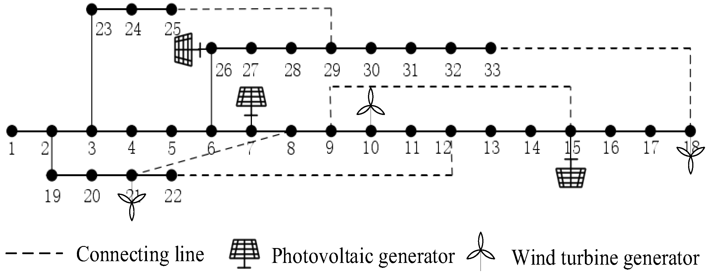
In this paper, the topology of the distribution network is described as an undirected network graph G = (V, E), where V contains all N nodes in the distribution network, v_i $\in$ V, and E represents the edge between nodes, which is the line of the distribution grid, (v_i, v_j) $\in$ E. In addition, the topology structure of the distribution network is analyzed by using the undirected network diagram to represent the structural information. Based on this, to process the irregular non-Euclidean structured data, the GAT is adopted to capture complex relationships between nodes in the distribution network through graph methods, such as the connection methods between nodes, and learn different importance weights between nodes through attention mechanisms. The GAT algorithm excels at preserving the integrity of original data, minimizing information loss and distortion. Additionally, it effectively captures the intricate topology and electrical attributes within the distribution network. Consequently, it provides a deeper insight into the system’s operational status and potential hazards. During the ADNDR process, the layout of the distribution network undergoes constant alterations. GATs possess a specific level of flexibility, enabling them to address these changes in the network’s layout to a certain degree. This characteristic facilitates real-time surveillance of the distribution network and aids in devising reconfiguration strategies.

The input of the GAT is I = (G, X), where $X=\left(x_1,x_2,\dots x_N\right)\in R^{N\times C}$ is the eigenvector matrix of each node and G = (V, E) is the undirected graph corresponding to the distribution network, where N is the number of nodes and C is the eigenvector dimension of each node. To improve the expression ability of each node’s features, the GAT uses a self-attention mechanism for each node, with a self-attention coefficient of:

$$e_{ij}=a\left(W{x}_i,W{x}_j\right)$$

(14)

where a is a single-layer feedforward neural network; x_i and x_j are the feature vectors of node i and node j, respectively; and W is the weight matrix. Unlike the global attention mechanism, which considers all positional information of feature vectors, the GAT employs a masked attention mechanism. This mechanism focuses only on partial positional information; specifically, it only computes the e_ij for the first-order neighboring nodes of node i and normalizes the attention coefficients of different nodes using the softmax function to obtain normalized coefficients ${\alpha }_{ij}$. These normalized coefficients ${\alpha }_{ij}$ are then used to compare the attention coefficients among different nodes. The expression is as follows:

$${\alpha }_{ij}=\mathrm{soft}\max \left(e_{ij}\right)={\displaystyle \frac{\exp \left(e_{ij}\right)}{{\displaystyle {\sum }_{k\in N_i}\exp \left(e_{ik}\right)}}}$$

(15)

After obtaining the normalization coefficient ${\alpha }_{ij}$, a nonlinear activation function is used to update the node’s own features as output by linearly combining the features of adjacent nodes:

$${x^{\prime }}_i=\sigma \left({\displaystyle \sum _{j\in N_i}{\alpha }_{ij}W{x}_j}\right)$$

(16)

where N_i is the set of adjacency matrices for node i, and $\sigma (\cdot )$ is a nonlinear activation function. To enhance the stability of the self-attention learning process, the GAT employs a multi-head attention mechanism. This mechanism involves combining K separate attention mechanisms. After transforming the node features according to the aforementioned process, these mechanisms are concatenated to produce updated node output features. The resulting output features are as follows:

$$x_i^{\prime }={\Vert }_{k=1}^K\sigma \left({\displaystyle \sum _{j\in N_i}{\alpha }_{ij}^k{W}^k{x}_j}\right)$$

(17)

4.2. Deep Deterministic Policy Gradient (DDPG)

The ADNDR model for an active distribution network, which is dynamic in nature, poses a challenging high-dimensional, mixed-integer, nonlinear optimization problem that incorporates stochastic elements. Traditional optimization techniques, including mathematical algorithms and heuristic methods, face challenges in addressing this intricate problem, particularly regarding computational efficiency and precision. DRL interacts with its environment to continually refine behavioral strategies. Its ultimate goal is to secure the highest possible long-term average cumulative rewards, along with the respective optimal strategies. It also utilizes deep neural network approximation functions and policy functions to handle more complex state and action spaces, improving the applicability and performance of the algorithm.

The DRL algorithm has four advantages in solving the ADNDR problem: (1) The DRL algorithm has strong adaptability to uncertain factors. Traditional mathematical optimization algorithms have many shortcomings in dealing with uncertain factors, while DRL algorithms can learn and formulate optimal strategies in uncertain environments through interaction and feedback with the environment, thus adapting well to changes in uncertain factors. (2) The DRL algorithm does not require predicting load and renewable energy output. At present, most algorithms are based on distributed energy and load prediction data for ADNDR [15,16]. However, there exists a degree of discrepancy between the forecasted data and the real-world scenario. This discrepancy has the potential to trigger operational hazards, including voltage deviations beyond acceptable limits, excessive power loads, and heightened network losses. During the actual implementation of the reconfiguration strategy, these risks may manifest. The DRL algorithm possesses the capability to directly derive decisions from the present system state and the associated action value functions. Consequently, forecasting renewable energy and load output becomes unnecessary. (3) The DRL algorithm does not require distribution network parameters for model construction. For complex distribution network structures, parameter acquisition is often not directly possible, while the DRL algorithm can learn directly from the environment and find the optimal decision action through reward and punishment signal feedback from the environment, which belongs to a model-free algorithm. (4) The DRL algorithm takes into account the long-term returns associated with the operation of the distribution network. In the dynamic reconfiguration problem of active distribution networks, the state of the distribution network changes dynamically, including changes in load, topology, etc. The objective function is usually described as cumulative benefits over some time, as shown in Equations (1)–(4). DRL determines the most suitable reconfiguration strategy by taking into account long-term benefits and possessing a level of dynamic adaptability. This enables it to tackle the sequential decision-making optimization challenge in dynamic distribution networks efficiently, ultimately fulfilling the long-term operational requirements of these networks more effectively. In summary, the DRL algorithm is very suitable for solving the ADNDR problem.

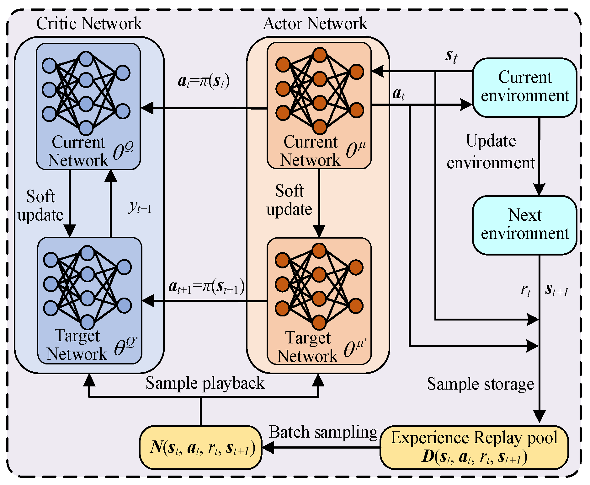
Based on how intelligent agents make choices, reinforcement learning algorithms can be categorized into three distinct types. These include algorithms that are value-based, those that are policy-based, and those that integrate both value and policy considerations. Value-based algorithms are often able to better utilize data and learn more accurate estimates of value functions. Policy-based algorithms can often better explore the action space by directly parameterizing policies. The DDPG algorithm is seen as a combination of value-based and policy-based algorithms, which update parameters through approximation functions and deterministic strategies. Hence, it integrates the swift convergence characteristics of policy-based algorithms with the stability and reliable convergence traits of value-based approaches. The DDPG algorithm, utilizing the actor–critic architecture, is capable of efficiently leveraging data throughout the learning phase. It achieves a balance between exploring new possibilities and utilizing known information. The structure diagram of DDPG is demonstrated in Figure 2. In Figure 2, it can be found that the DDPG model consists of two neural networks: one actor network ${\theta }^{\mu }$ is used to decide the action at the current moment, and the other critic network ${\theta }^Q$ is used to estimate the action value function and the quality of the current state value. DDPG stores all transition states (s_t, a_t, r_t, s_t+1) experienced in the experience replay pool D, where s_t represents the current state, a_t represents the current action, r_t represents the reward function value, and s_t+1 represents the next state.

The actor policy network in DDPG is divided into the current network ${\theta }^{\mu }$ and the target network ${\theta }^{{\mu }^{\prime }}$. The current network ${\theta }^{\mu }$ selects the optimal action based on the current state s_t provided by the environment, thereby generating the next state s_t+1, obtaining a reward r_t, and updating the current network parameters ${\theta }^{\mu }$ based on the Q value calculated by the critic network ${\theta }^Q$. The target network selects the optimal next action a_t+1 based on the next state s_t+1 sampled from the experience replay pool. The target network parameters ${\theta }^{{\mu }^{\prime }}$ are updated at fixed intervals based on the current network parameters ${\theta }^{\mu }$.

For the actor architecture, traditional implementations employ MLPs to process state features. In contrast, our GAT-DDPG framework introduces Graph Attention Layers to model state representations as graph-structured data. Specifically, the GAT dynamically assigns attention weights to neighboring nodes through learnable coefficients, enabling the actor to focus on critical interactions (e.g., agent dependencies in multi-agent systems) while filtering irrelevant connections. This replaces MLP’s fixed-weight aggregation with adaptive relational reasoning, significantly enhancing action generation in environments with implicit or evolving dependencies.

The critic network in DDPG is divided into the current network ${\theta }^Q$ and the target network ${\theta }^{{\mu }^{\prime }}$. The current network ${\theta }^Q$ calculates the current Q value $Q\left(s_t,a_t,{\theta }^Q\right)$ based on the action a_t selected by the actor current network ${\theta }^{\mu }$ and the current state s_t, which is used to update the actor’s current network parameters and the commentator’s current network parameters ${\theta }^Q$. The target network is responsible for calculating $Q^{\prime }\left(s_{t+1},a_{t+1},{\theta }^{Q^{\prime }}\right)$ in the target Q value y_i, and the expression for the target Q value y_i is as follows:

$$y_i=r_t+\gamma Q^{\prime }\left(s_{t+1},a_{t+1},{\theta }^{Q^{\prime }}\right)$$

(18)

where y_i is the target Q value; $\gamma$ is the attenuation factor; and $Q^{\prime }\left(s_{t+1},a_{t+1},{\theta }^{Q^{\prime }}\right)$ is the Q value calculated by the target critic network ${\theta }^{Q^{\prime }}$ based on the next state s_t+1 and the optimal action a_t+1. The network parameters ${\theta }^{{\mu }^{\prime }}$ are updated at fixed intervals based on the current network ${\theta }^{\mu }$.

Unlike standard DDPG, where the critic concatenates state–action vectors as MLP inputs, our GAT-based critic constructs a hybrid graph where nodes encode state features and edges integrate action attributes. GAT layers propagate features across this graph, computing attention-based Q-values that capture both local action impacts and global interactions (e.g., long-term dependencies in continuous control tasks). This design ensures nuanced modeling of state–action interdependencies, particularly in partially observable environments.

The goal of the actor network in DDPG is to obtain a larger Q value as much as possible, and the smaller the feedback Q value obtained, the greater the loss. Therefore, as long as a negative sign is taken on the Q value returned by the commentator’s current network ${\theta }^Q$, it is called the loss function, and its expression is as follows:

$$J\left({\theta }^{\mu }\right)=-{\displaystyle \frac{1}{m}}{\displaystyle \sum _{i=1}^{m}Q\left(s_t,a_t,{\theta }^Q\right)}$$

(19)

where $J\left({\theta }^{\mu }\right)$ is the loss function value of the actor current network ${\theta }^{\mu }$; m is the number of samples with batch gradient descent; and $Q\left(s_t,a_t,{\theta }^Q\right)$ is the Q value calculated by the critic network ${\theta }^Q$ based on the current state s_t, current action a_t, and current network parameters ${\theta }^Q$. The actor current network ${\theta }^{\mu }$ updates the network parameters using a backpropagation algorithm based on the loss function.

The commentator in DDPG’s current network ${\theta }^Q$ loss function is a mean square error, which is expressed as follows:

$$J\left({\theta }^Q\right)={\displaystyle \frac{1}{m}}{\displaystyle \sum _{i=1}^m{\left(y_i-Q\left(s_t,a_t,{\theta }^Q\right)\right)}^2}$$

(20)

where $J\left({\theta }^Q\right)$ is the loss function value of the commentator’s current network ${\theta }^Q$; m is the number of samples with batch gradient descent; y_i is the target Q value; and $Q\left(s_t,a_t,{\theta }^Q\right)$ is the Q value calculated by the critic’s network ${\theta }^Q$ based on the current state s_t, current action a_t, and current network parameters ${\theta }^Q$. The critic current network ${\theta }^Q$ uses a backpropagation algorithm to update network parameters based on this loss function.

The soft-update technique is utilized for modifying the settings of the actor target network, as detailed below:

$${\theta }^{{\mu }^{\prime }}\leftarrow \tau {\theta }^{\mu }+\left(1-\tau \right){\theta }^{{\mu }^{\prime }}$$

(21)

where $\tau$ is the update coefficient, and in this paper, $\tau =0.01$ is used.

5. An ADNDR Method Based on GATDDPG

The complexity of the distribution network leads to a situation where the interconnections among nodes play a crucial role in determining the power system’s stability. Furthermore, these connections have a profound impact on its reliability. The GAT excels in handling graph-structured data with complex topological structures, while DDPG is an efficient reinforcement learning algorithm that can learn efficient and stable reconfiguration strategies by exploring in the distribution network environment. Therefore, the research presented in this paper introduces a novel approach to ADNDR, utilizing the GATDDPG framework. By introducing the GAT to process graph structure information in the environment, the proposed algorithm can more accurately understand the dynamics and relationships of the environment. Meanwhile, by leveraging DDPG for optimizing and rearranging the decision-making procedure, we can guarantee the agent acquires strategies that are both stable and effective. This section constructs a reinforcement learning model for the ADNDR strategy based on GATDDPG, as shown in Figure 3.

The Markov decision process (MDP) is aimed at making decisions through a random program with Markov properties [17]. The MDP provides a solid theoretical foundation for reinforcement learning, allowing us to make optimal decisions while considering the current state and possible future changes in the distribution network. By modeling the distribution network reconfiguration problem as the MDP, we can effectively utilize the GATDDPG algorithm to search and learn the optimal distribution network reconfiguration strategy. The following describes the MDP model for ADNDR, including the state s_t, action a_t, and reward function r_t.

5.1. State

The state s_t = (G_t, X_t) includes the topology diagram G_t and distribution network node characteristic (voltage, power, etc.) information $X_t\in R^{N\times C}$ at time t. C is the number of features of the node, where C = 3; N is the number of distribution network nodes, where N = 33.

(1)

The distribution network topology diagram G_t represents the connection relationship of nodes in the distribution network at time t.

(2)

The node feature matrix X_t represents the node feature information of the distribution network at time t, and each row represents a node feature vector. Its expression is as follows:

$$X_t=\left\{P_t,Q_t,V_t\right\}$$

(22)

where P_t and Q_t are the sets of active and reactive power of each node at time t, respectively, and V_t is the set of voltages at each node at time t. In this study, X_t was calculated using the Newton–Raphson method, a robust iterative algorithm widely adopted in power system analysis for solving nonlinear power flow equations. By iteratively linearizing nonlinear equations using Taylor series expansion (ignoring higher-order terms), it converts the problem into solving a series of linear matrix equations (e.g., Jacobian matrix updates) until convergence.

5.2. Action

The action generally refers to the strategies or behaviors that intelligent agents can adopt. On this basis, the intelligent agent selects a certain action to execute in the action space based on the state s_t, that is:

$$a_t=k,\hspace{1em}k\in S_{\mathrm{cheme}}$$

(23)

Equation (23) indicates that the agent selects an action a_t from the action space S_cheme. In our study, the action is chosen based on the encoding technique outlined in Section 2. Specifically, there are 732 viable options available, meaning we select one of these 732 solutions for execution. For example, in the IEEE 33-bus power system shown in Figure 1, if a selected five-dimensional action vector is {0, 1, 0, 2, 3}, as shown in Table 3, the action scheme represents the disconnection of branch 3, branch 8, branch 9, branch 18, and branch 35 and the closure of other remaining branches in the distribution network.

5.3. Reward Function

The reward function constitutes a fundamental element in reinforcement learning algorithms. It outlines the agent’s learning goal, namely, achieving the highest possible accumulation of rewards. This paper transforms the objective function in the mathematical model of distribution network reconfiguration in Section 2 into a reward function to reduce network loss and voltage offset, which is helpful for the training of intelligent agents. At the same time, it is necessary to ensure that the ADNDR solution of the agent can satisfy all constraint conditions; otherwise, the results of distribution network reconfiguration will be meaningless. Therefore, this paper establishes the following reward function:

$$r_t=\left\{\begin{array}{l}-f_{\mathrm{ADNDR}} , f_{\mathrm{success}}=1\\ -3 , f_{\mathrm{success}}=0\end{array}\right.$$

(24)

where r_t is the reward value for executing action a_t based on state s_t at time t; when f_success = 1, it indicates that the proposed reconfiguration scheme fully complies with all the established constraint conditions in the ADNDR mathematical model, specifically encompassing the contents described in Equations (7) to (13). At this point, the reward value will be calculated normally according to the established rules. Conversely, if f_success = 0, it implies that the reconfiguration scheme fails to fully meet the constraint conditions in the mathematical model. In this unfavorable scenario, in order to guide the agent to avoid such schemes in future decisions, we will impose a significant penalty on the agent, which is set to −3 in this study.

5.4. Solving Process

A GATDDPG algorithm was developed for addressing the challenge of ADNDR. This allows us to attain the best approach for rearranging the network configuration. The procedure for dynamically reconfiguring an active distribution network while considering graph structure information is depicted in Figure 4. Below are the detailed steps involved in this process:

• Step 1: Initialize the current network parameters ${\theta }^{\mu }$ of actors, actor target network ${\theta }^{{\mu }^{\prime }}$, commentator current network parameters ${\theta }^Q$, commentator target network parameters ${\theta }^{Q^{\prime }}$, and iteration number e in GATDDPG and determine the maximum iteration number E and maximum random exploration number M.
  Step 2: Adopt a coding method based on basic circuits to reduce the action space of ADNDR.
  Step 3: Initialize the time identifier t.
  Step 4: Initialize the distribution network and obtain the voltage, active power, and reactive power of each node according to Equation (22), as well as the distribution network structure diagram G_t. Construct the initial state space s_t = (G_t, X_t).
  Step 5: If the number of iterations is less than the maximum number of random explorations M, the actor adopts a random policy. If the number of iterations is greater than the maximum number of random explorations M, the actor network ${\theta }^{\mu }$ selects the optimal action a_t based on the current distribution network state s_t.
  Step 6: According to action a_t, disconnect the corresponding switch in the distribution network and reconfigure the network.
  Step 7: Perform power flow calculation on the reconfigured distribution network, obtain the reconfigured state space s_t+1, and calculate the reward function value r_t according to Equation (24).
  Step 8: Store the pre-refactoring state s_t, refactoring action a_t, corresponding reward function value r_t, and the refactored state s_t+1 in the experience replay pool D.
  Step 9: If the number of iterations is greater than the number of random explorations M, proceed to step 10. If the number of iterations is less than the random exploration number M and the time identifier is less than 24, update the time and return to step 5. If the iteration count is less than the random exploration count M and the time identifier is greater than or equal to 24, update the iteration count and return to step 3.
  Step 10: Batch sample m samples {s_t, a_t, r_t, s_t+1} from the experience replay pool.
  Step 11: Use the commentator to calculate the Q value between the current network ${\theta }^Q$ and the target network ${\theta }^{Q^{\prime }}$ based on Equation (18) and the loss function value through Equations (19) and (20) based on the Q value. Update the network parameters using the backpropagation algorithm. When the time identifier reaches 24, execute step 12. Otherwise, update the time and execute step 5.
  Step 12: Terminate the training process once the predefined maximum iteration limit is attained. If not, increment the iteration count and advance to the next step, which is step 3.

6. Case Study

6.1. Simulation Environment Settings

This paper presents an enhanced version of the IEEE 33-bus power system, specifically tailored for case studies, which is depicted in Figure 5. The IEEE 33-bus power system consists of 1 substation and 37 branches, with a voltage range of 0.9~1.1 during normal operation. In this paper, H_SWI,max and H_SWI,b,max are set to 15 and 3, respectively [18]. The basic branch and load information in the IEEE’s 33 nodes can be found in reference [19]. The permissible capacity limits of the branches strictly adhere to the values documented in [14] (Table 1) to ensure operational safety constraints. The wind turbines with rated powers of 600 kW, 1100 kW, and 1000 kW are installed at nodes 10, 18, and 21 of the IEEE 33-bus power system, respectively. Photovoltaic generators with rated powers of 600 kW, 1100 kW, and 1000 kW are installed at nodes 7, 15, and 26 of the IEEE 33-bus power system, respectively. And the power factors are set as 0.9. The 24 h photovoltaic generation, wind turbine, and load power curves depicted in Figure 6 are long-term averaged profiles derived from multi-year historical data (2015–2024) via the Xihe Energy Big Data Platform [20]. The photovoltaic curves integrate hourly solar irradiance and temperature data calibrated with the DISC model to account for spectral variations and panel efficiency degradation, while the wind power curves incorporate aerodynamic corrections and air density adjustments based on altitude and temperature. The load profiles reflect regional demand patterns synthesized from industrial, commercial, and residential consumption trends, excluding extreme weather scenarios. During training, stochastic fluctuations (±5%) are superimposed on these averaged curves to simulate real-time uncertainties while maintaining physical feasibility.

6.2. Simulation Parameter Settings

The parameters and neural network model of GATDDPG are shown in

Table 4. Parameters of GATDDPG algorithms.

Parameter	Value
Learning rate	5 × 10−5
Discount factor	0.9
Training batch size	64
Storage capacity	10,000
Iterations	1000
Random exploration times	300

and

Table 5. The structure and activation function of the neural network in GATDDPG.

Network Layer	Actor		Critic
	Neural Network Structure	Activation Function	Neural Network Structure	Activation Function
Input layer	33 × 3	/	33 × 3	/
GAT1	3 → 32	ReLU	3 → 32	ReLU
GAT2	32 → 16	ReLU	32 → 16	ReLU
FC1	33 × 16 → 64	ReLU	33 × 16 + naction → 64	ReLU
FC2 (output layer)	64 → naction	softmax	64→1	/

. It can be found in Table 5 that the actor network ${\theta }^{\mu }$ consists of an input layer, three hidden layers, and one output layer. In the input layer, the state includes active power, reactive power, and the voltage of all nodes, whose dimension is 33 × 3. Thus, the input layer of the actor network is a 33 × 3 graph feature matrix, which is activated by two GAT layers and ReLU functions and then by two FC layers to finally output the policy function of the current state.

The critic network ${\theta }^Q$ in this paper consists of one input layer, three hidden layers, and one output layer. The input layer is also a 33 × 3 graph feature matrix, which is activated by two layers of GAT and ReLU functions and then by two layers of fully connected (FC) layers to finally output the action value function of the current state.

6.3. Hyperparameter Measurement

The determination of the learning rate along with the discount factor has a substantial influence on the efficacy of agent training. Consequently, it is necessary to conduct a thorough examination and contrast of these parameters to ascertain the most suitable hyperparameter setup. The reward function values of GATDDPG under different learning rates and discount factors are presented in

Table 6. Comparison of evaluation indicators for different hyperparameters.

Algorithms	Learning Rate	Discount Factor	Reward
GATDDPG	5 × 10−5	0.85	−3.6544
	5 × 10−5	0.9	−2.3621
	5 × 10−5	0.95	−3.1141
	5 × 10−6	0.95	−3.5194
	5 × 10−4	0.95	−2.5413

. Meanwhile, the optimization results of GATDDPG under different learning rates and discount factors are shown in Figure 7 and Figure 8. Observing Figure 7, it is evident that when the learning rate is set to 5 × 10⁻⁶, the optimization effectiveness of the GATDDPG algorithm is not ideal, attributed to the excessively low learning rate, which results in a small step size during parameter updates, making it difficult to effectively capture gradient information. However, when the learning rate is set to 5 × 10⁻⁵ and 5 × 10⁻⁶, GATDDPG exhibits good optimization performance. Among them, it is clear from Table 6 that the reward function value at a learning rate of 5 × 10⁻⁵ is higher than that at a learning rate of 5 × 10⁻⁶. Therefore, the final learning rate for GATDDPG is determined to be 5 × 10⁻⁵. Observing Figure 8, when the discount factor is set to 0.95, the GAT requires a longer training period to achieve convergence of the reward function value, due to the excessively high discount factor, which makes the algorithm overly focused on long-term rewards while neglecting near-term feedback. In contrast, the GATDDPG algorithms with discount factors of both 0.9 and 0.85 exhibit good optimization performance. Among them, the network with a discount factor of 0.9 converges slightly faster than that with 0.85. And it is clear from Table 6 that the reward function value at a discount factor of 0.9 is higher than that at a discount factor of 0.85. However, it should be noted that although the discount factor of 0.95 performs poorly in the early stages of training, its long-term performance may be better, requiring a trade-off based on specific application scenarios. However, based on the current data and requirements, the final discount factor is determined to be 0.9. In summary, the learning rate of the GATDDPG network used in this paper is finally set to 5 × 10⁻⁵, and the discount factor is set to 0.9.

6.4. Comparative Analysis of Network Loss and Voltage Under Different Algorithms

To showcase the efficacy and advantage of our GATDDPG-inspired optimization method for ADNDR strategies, the present section evaluates its performance by contrasting it with four alternative optimization algorithms, all in the context of tackling ADNDR strategy optimization challenges. Specifically, these algorithms include the MISOCP algorithm, the standard DDPG algorithm, the GATDDQN algorithm, and the GCNDDPG algorithm.

Firstly, we aim to showcase the viability of employing deep neural networks for approximating the action value function. To this end, Figure 9 presents the loss function values obtained using various algorithms. Since the training of the neural network only starts from the 300th episode, the range of episode values is from 300 to 1000.

From Figure 9, it can be seen that the loss functions of the neural networks of each DRL algorithm can effectively converge, and their training process is fast and stable. Therefore, deep neural networks can accurately predict the action value function in various DRL algorithms.

Furthermore, to rigorously evaluate the effectiveness of the GATDDPG-based approach for ADNDR, we undertook a comparative study. This involved assessing the performance of multiple algorithms in tackling ADNDR challenges. Specifically, the reward function values under different algorithms are shown in Figure 10, while a comparison of the evaluation indicators for different algorithms is presented in

Table 7. Comparison of evaluation indicators for different algorithms.

Algorithms	Reward	Training Time/h	Decision Time/s
Original network	−5.0478	/	/
MISOCP	−2.2263	/	34.94
DDPG	−3.6378	2.08	0.142
GATDDQN	−3.3293	1.33	0.130
GCNDDPG	−2.7082	1.82	0.133
GATDDPG (The proposed method)	−2.3615	0.78	0.111

. To quantitatively validate the effectiveness of the GATDDPG-based approach (ADNDR), a comparative analysis of various algorithms’ performance on ADNDR was conducted, as illustrated in Figure 10 and summarized in Table 7.

Based on the various algorithms, the ADNDR strategy is capable of enhancing the performance metrics of the distribution network. Specifically, it improves network loss and reduces voltage deviation, as illustrated in Figure 10. The ADNDR strategy utilizing GATDDQN exhibits relatively sluggish reward convergence. In contrast, the ADNDR strategy leveraging GCNDDPG achieves faster convergence, albeit with a reward function that slightly underperforms compared to the ADNDR strategy grounded in GATDDPG presented herein.

From Table 7, we can conclude the following:

(1)

In terms of reward values, the reward function of GATDDPG exhibits higher numerical values compared to GATDDQN, indicating that the DDPG algorithm has advantages in optimization performance over the DDQN algorithm. Furthermore, both GATDDPG and GCNDDPG surpass the traditional DDPG in terms of reward values, demonstrating the necessity and effectiveness of considering graph structure information when solving the ADNDR problem. Specifically, the reward value of GATDDPG reaches −2.3615, achieving a 12.8% improvement compared to the −2.7082 of GCNDDPG, which strongly proves that using the GAT to fit the action-value function is superior to the GCN.

(2)

In terms of computing speed, the training time of GATDDPG is 0.68 h, which is reduced by 48.8%, 63.6%, and 12.8% compared to the training time of DDPG, GATDDQN, and GATDDPG, respectively. The decision times of GATDDPG, GCNDDPG, GATDDQN, DDPG, and MISOCP are 0.111 s, 0.133 s, 0.130 s, 0.142 s, and 34.94 s, respectively. Compared with GCNDDPG, GATDDQN, DDPG, and MISOCP, the decision time of GCNDDPG is reduced by 16.5%, 14.6%, 21.8%, and 99.68%, respectively.

(3)

In terms of constraint conditions, based on the definition in Equation (24), this study assigns a penalty factor of −3 to reconfiguration schemes that fail to meet the constraints within each time step. During the random exploration phase, the agent adopts a strategy of randomly selecting actions, which may result in the selected actions not fully complying with all constraints, thereby causing a significant decrease in the cumulative reward function value, specifically to around −60. However, upon entering the optimization phase, except for the GATDDQN algorithm, the 24 h cumulative reward function values of the other algorithms stabilize near −3. This phenomenon indicates that the reward function value at each time step exceeds −3, implying that the penalty term is not activated. Therefore, we can reasonably infer that the GATDDPG-based ADNDR strategy can effectively satisfy all the constraint conditions listed in the mathematical model (i.e., Equations (7)–(13)).

To validate the effectiveness of the proposed method, this study systematically compared the performance differences of various algorithms across key metrics, including daily average network loss, voltage deviation, node voltage distribution at 12:00, and dynamic network loss, with the experimental results illustrated in Figure 11, Figure 12 and Figure 13. Data analysis reveals the following: Under the benchmark scenario, the distribution network exhibited daily average network loss and voltage deviation of 135.0650 kW and 0.8073 p.u., respectively. The DDPG algorithm reduced these metrics to 77.3583 kW and 0.7451 p.u. (reductions of 42.73% and 7.70%), while GATDDQN and GCNDDPG further optimized them to 65.2251 kW/0.4697 p.u. (reductions of 51.71%/41.82%) and 67.3276 kW/0.5862 p.u. (reductions of 50.15%/27.39%), respectively. Although all aforementioned DRL algorithms improved network performance, their optimization margins differed significantly.

Notably, the GATDDPG-based ADNDR strategy achieved the highest reductions in both metrics (51.71% network loss and 41.82% voltage deviation), outperforming the conventional DRL methods. In contrast, the MISOCP mathematical optimization method further reduced the metrics to 63.9830 kW/0.5071 p.u. (reductions of 52.63%/37.18%), but at the cost of significantly degraded computational efficiency—its solving time grew exponentially with network scale, rendering it impractical for real-time optimization. The proposed method maintained competitive optimization performance (with only 0.92% and 4.64% gaps in network loss and voltage deviation compared to MISOCP) while reducing the computation time by two orders of magnitude. Furthermore, as illustrated in Figure 12 and Figure 13, in terms of node voltage stability, the method based on GATDDPG demonstrated superior performance compared to MISOCP. Additionally, Figure 14 shows that the network loss trajectory optimized by the reconstruction strategy based on GATDDPG was extremely close to the results obtained by MISOCP. These observations robustly validate the exceptional global optimization capability of the proposed method.

These experiments demonstrate that the GATDDPG-based ADNDR strategy effectively captures implicit topological correlations through graph attention mechanisms, achieving near-optimal control performance without requiring precise parameter identification. This provides a highly efficient and robust solution for real-time reconfiguration in large-scale active distribution networks.

As shown in

Table 8. Dynamic network reconfiguration strategy.

Time	Reconfiguration Switch
0:00–9:00	[37, 34, 13, 7, 8]
10:00–15:00	[27, 8, 13, 33, 9]
16:00–23:00	[37, 34, 13, 7, 8]

, a more in-depth analysis of the dynamic reconfiguration strategy was conducted. The topology reconfiguration strategy generated by ADNDR based on GATDDPG exhibits significant temporal variability in the switching combinations across different time intervals. Specifically, the switching configurations during the 10:00 to 15:00 period differ significantly from those in other time periods. This difference can be attributed to the significant fluctuations in PV output during the peak irradiation period (i.e., 10:00–15:00), as visually demonstrated by the PV generation curve in Figure 6.

Additionally,

Table 9. The number of switch actions corresponding to the dynamic network reconfiguration strategy.

Action Switch	Number of Switch Operations	Sum of Switch Operation Counts
b7	2	12
b9	2
b27	2
b33	2
b34	2
b37	2

illustrates the action switches involved in the reconfiguration strategy along with their corresponding action counts. In Figure 9, it can be observed that the action count for each individual switch is less than the maximum allowed action count for that switch (3 times/day), and the total action count for all switches is also less than the maximum total action count (15 times/day). This indicates that the ADNDR strategy based on GATDDPG can optimize network loss and voltage deviation in the distribution network while satisfying the constraints on switch action counts.

Furthermore, Figure 13 reveals that as the PV output increases, there is a sharp rise in distribution network voltage. This phenomenon prompts the GATDDPG algorithm to dynamically adjust and reconfigure its strategy by prioritizing voltage-sensitive nodes. This adaptive feature of the algorithm fully demonstrates its sensitivity to real-time operating conditions, thereby effectively ensuring voltage stability in environments with high renewable energy penetration rates.

6.5. Analysis of Adaptability to Uncertainty Factors

To further validate the superiority of the proposed ADNDR based on GATDDPG in dealing with uncertainties, we conducted a comparative analysis of the following four optimization strategies:

• Strategy 1: Without considering the uncertainties in load and DG output, the MISOCP algorithm was used to solve the ADNDR strategy.
• Strategy 2: Fully considering the uncertainties in load and DG output, the MISOCP algorithm was also employed to solve the ADNDR strategy.
• Strategy 3: Ignoring the uncertainties in load and DG output, the GATDDPG algorithm was utilized to solve the ADNDR strategy.
• Strategy 4: Taking into full account the uncertainties in load and DG output, the GATDDPG algorithm was applied to implement the solution for the ADNDR strategy.

The optimization results for each strategy are detailed in

Table 10. Reward function values for different optimization methods.

Strategy	Reward
Strategy 1	−2.0628
Strategy 2	−2.2263
Strategy 3	−2.4686
Strategy 4	−2.3615

. According to the data in Table 10, we can observe that in environments containing uncertainties, the reward function value of the MISOCP algorithm decreased from −2.0628 to −2.2263, representing a decline of 7.9%. In contrast, the optimization performance of the GATDDPG algorithm was not compromised by the presence of uncertainties in the environment. Instead, its reward function value increased, which strongly demonstrates the robust adaptability of the GATDDPG algorithm in dealing with uncertainties.

6.6. Impact of Operational Constraints on Network Reconfiguration Decision Consistency

To delve deeper into the specific impacts of constraints on reconfiguration strategies, this subsection employs the GATDDPG algorithm to solve the following four mathematical models:

• Model 1: Model 1 sets Equation (4) as the optimization objective, with Equations (7)–(11) serving as constraints. This model does not incorporate the constraints of switch operation frequency and branch transmission capacity.
• Model 2: Model 2 sets Equation (4) as the optimization objective and introduces Equations (7)–(11) and (13) as constraints. This model considers the constraint of branch transmission capacity but does not consider the constraint of switch operation frequency.
• Model 3: Model 3 sets Equation (4) as the optimization objective and specifies Equations (7)–(12) as constraints. This model considers the constraint of switch operation frequency but does not consider the constraint of branch transmission capacity.
• Model 4: Model 4 sets Equation (4) as the optimization objective, with Equations (7)–(13) serving as constraints. This model simultaneously considers the constraints of switch operation frequency and branch transmission capacity.

The solutions to these four mathematical models are detailed in

Table 11. Reward function values of different mathematical models.

Model	Reward
Model 1	−2.2043
Model 2	−2.2043
Model 3	−2.3615
Model 4	−2.3615

. Analysis of the data in Table 11 reveals that after considering the constraint of switch operation frequency, the reward function values of the reconfiguration strategies exhibit a downward trend, indicating that the constraint of the switch operation frequency has a significant impact on the distribution network reconfiguration strategies. However, when the number of switch operations in the distribution network exceeds a certain threshold, necessary maintenance or replacement operations are required. Therefore, although the reward function values derived from Models 1 and 2 are higher than those from Models 3 and 4, their reconfiguration strategies only possess theoretical exploration value and lack practical application significance due to their neglect of the switch operation frequency constraint. Furthermore, by comparing the solutions of Models 1 and 2, as well as Models 3 and 4, it can be observed that in the distribution network environment set in this paper, whether the constraint of branch transmission capacity is considered does not have a significant impact on reconfiguration strategies. However, this does not mean that considering the constraint of branch transmission capacity is unimportant, as it ensures the stable operation of the power grid within a safe range and effectively avoids potential risks such as overloading. In summary, the optimization method discussed in this paper can effectively optimize distribution network reconfiguration strategies under the premise of satisfying the constraints of the switch operation frequency and branch transmission capacity, providing a decision support tool that balances safety and economy for active distribution networks with a high proportion of renewable energy.

7. Conclusions

This research presents a dynamic adjustment approach for active distribution networks, utilizing the GATDDPG algorithm as its foundation. The method focuses on reconfiguring the network efficiently. This algorithm effectively combines the data processing ability of a GAT graph with the decision-making ability of DDPG. The main conclusions are as follows:

(1)

Compared with the traditional encoding methods, the loop-based encoding method used in this paper greatly reduces the number of feasible solutions by 95.53%, indicating that this encoding method has higher solving efficiency.

(2)

Compared with the DDPG-based ADNDR strategy, the proposed GATDDPG-based ADNDR strategy reduces network loss and voltage offset by 8.98% and 19.69%, respectively. This demonstrates that considering graph structure information is very effective in solving ADNDR.

(3)

Compared with the ADNDR strategy based on GCNDDPN, the proposed ADNDR strategy based on GATDDPG reduces network loss and voltage offset by 1.56% and 14.43%, respectively. This indicates that, compared to using the GCN, using the GAT as a function fitting tool for graph reinforcement learning algorithms in solving ADNDR problems is more effective.

(4)

Compared with the ADNDR strategy based on GCNDDPG, GATDDQN, DDPG, and MISOCP, the ADNDR strategy based on GATDDPG reduces the decision time by 16.5%, 14.6%, 21.8%, and 99.68%, respectively, indicating that this method has higher reconfiguration efficiency.

In summary, the proposed ADNDR strategy based on GATDDPG can better adapt to distribution networks containing DGs. At present, most research focuses on the economic or reliability optimization of distribution networks. In the future, our work will focus on the synergistic optimization of economics and reliability in distribution networks and solving more complex ADNDR problems.

References

1. Zhang, Y.; Zeng, B.; Zhou, Y.; Xu, H.; Liu, W. Research on interactive integrated planning of data center and distribution network driven by carbon emission reduction. Trans. China Electrotech. Soc. 2023, 38, 6433–6450. [Google Scholar] [CrossRef]
2. Stojanović, B.; Rajić, T.; Šošić, D. Distribution network reconfiguration and reactive power compensation using a hybrid Simulated Annealing–Minimum spanning tree algorithm. Int. J. Electr. Power Energy Syst. 2023, 147, 108829. [Google Scholar] [CrossRef]
3. Yan, X.; Zhang, Q. Research on Combination of Distributed Generation Placement and Dynamic Distribution Network Reconfiguration Based on MIBWOA. Sustainability 2023, 15, 9580. [Google Scholar] [CrossRef]
4. Mi, Y.; Chen, Y.; Yuan, M.; Li, Z.; Tao, B.; Han, Y. Multi-timescale optimal dispatching strategy for coordinated source-grid-load-storage interaction in active distribution networks based on second-order cone planning. Energies 2023, 16, 1356. [Google Scholar] [CrossRef]
5. Ma, C.; Wang, D.; Shan, X.; Wu, H.; Xu, X.; Wang, Y.; Guo, Y.; Zhang, J. A fault recovery strategy of distribution network based on mixed-integer second-order cone programming. In Proceedings of the 2020 5th Asia Conference on Power and Electrical Engineering (ACPEE), Chengdu, China, 4–7 June 2020; IEEE: Piscataway, NJ, USA, 2020; pp. 1584–1589. [Google Scholar] [CrossRef]
6. Kazemi-Robati, E.; Sepasian, M.S. Fast heuristic methods for harmonic minimization using distribution system reconfiguration. Electr. Power Syst. Res. 2020, 181, 106185. [Google Scholar] [CrossRef]
7. Essallah, S.; Khedher, A. Optimization of distribution system operation by network reconfiguration and DG integration using MPSO algorithm. Renew. Energy Focus 2020, 34, 37–46. [Google Scholar] [CrossRef]
8. Wang, B.; Zhu, H.; Xu, H.; Bao, Y.; Di, H. Distribution network reconfiguration based on NoisyNet deep Q-learning network. IEEE Access 2021, 9, 90358–90365. [Google Scholar] [CrossRef]
9. Li, Y.; Hao, G.; Liu, Y.; Yu, Y.; Ni, Z.; Zhao, Y. Many-objective distribution network reconfiguration via deep reinforcement learning assisted optimization algorithm. IEEE Trans. Power Deliv. 2021, 37, 2230–2244. [Google Scholar] [CrossRef]
10. Veličković, P.; Cucurull, G.; Casanova, A.; Romero, A.; Lio, P.; Bengio, Y. Graph attention networks. arXiv 2017, arXiv:1710.10903. [Google Scholar] [CrossRef]
11. Liu, Z.; Liu, Y.; Xu, H.; Liao, S.; Zhu, K.; Jiang, X. Dynamic economic dispatch of power system based on DDPG algorithm. Energy Rep. 2022, 8, 1122–1129. [Google Scholar] [CrossRef]
12. Tavana, M.; Soltanifar, M.; Santos-Arteaga, F.J. Analytical hierarchy process: Revolution and evolution. Ann. Oper. Res. 2023, 326, 879–907. [Google Scholar] [CrossRef]
13. Xu, C.; Dong, S.; Zhu, J.; Zhu, B.; Xu, L. A radial constraint description method for distribution networks based on non connected power supply loop conditions. Autom. Electr. Power Syst. 2019, 43, 82–89. [Google Scholar] [CrossRef]
14. Trivić, B.; Savić, A. Optimal Allocation and Sizing of BESS in a Distribution Network with High PV Production Using NSGA-II and LP Optimization Methods. Energies 2025, 18, 1076. [Google Scholar] [CrossRef]
15. Bahrami, S.; Chen, Y.C.; Wong, V.W.S. Dynamic Distribution Network Reconfiguration with Generation and Load Uncertainty; IEEE: Piscataway Township, NJ, USA, 2024. [Google Scholar] [CrossRef]
16. Yang, X.; Wang, L. Probabilistic Power Flow Based Distribution Network Optimization with Distributed Generation. Acta Energ. Solaris Sin. 2021, 42, 71–76. [Google Scholar] [CrossRef]
17. Maran, D.; Olivieri, P.; Stradi, F.E.; Urso, G.; Gatti, N.; Restelli, M. Online markov decision processes configuration with continuous decision space. Proc. AAAI Conf. Artif. Intell. 2024, 38, 14315–14322. [Google Scholar] [CrossRef]
18. Cong, P.; Tang, W.; Lou, C.; Zhang, B.; Zhang, L. Two-stage coordinated optimal control of flexible soft open points and tie switches in active distribution networks with high penetration of renewable energy. Trans. China Electrotech. Soc. 2019, 34, 1263–1272. [Google Scholar] [CrossRef]
19. Shin, M.J.; Choi, D.H.; Kim, J. Cooperative management for PV/ESS-enabled electric vehicle charging stations: A multiagent deep reinforcement learning approach. IEEE Trans. Ind. Inform. 2019, 16, 3493–3503. [Google Scholar] [CrossRef]
20. Xihe. Energy Meteorological Big Data Platform [DB]. Available online: https://xihe-energy.com (accessed on 10 February 2025).
Figure 1. IEEE 33-bus power system branch encoding diagram.
Energies 18 02080 g001
Figure 2. DDPG structure diagram.
Energies 18 02080 g002
Figure 3. Structure diagram of the ADNDR strategy based on GCNDDPG.
Energies 18 02080 g003
Figure 4. Flowchart of the dynamic reconfiguration algorithm for active distribution networks.
Energies 18 02080 g004
Figure 5. Schematic diagram of an improved IEEE 33-bus system.
Energies 18 02080 g005
Figure 6. The 24 h DG active power and load curves.
Energies 18 02080 g006
Figure 7. Optimization results under different learning rates.
Energies 18 02080 g007
Figure 8. Optimization results under different discount factors.
Energies 18 02080 g008
Figure 9. Value of the loss function under different algorithms.
Energies 18 02080 g009
Figure 10. Reward function values under different algorithms.
Energies 18 02080 g010
Figure 11. Daily average network loss and voltage deviation for different algorithms.
Energies 18 02080 g011
Figure 12. Voltage at each node at 12:00 for different algorithms.
Energies 18 02080 g012
Figure 13. Average node voltage of different algorithms at different times.
Energies 18 02080 g013
Figure 14. Network loss at various time points for different algorithms.
Energies 18 02080 g014