Abstract
The increasing penetration of renewable energy sources (RESs) has reduced the inertia and reserve levels of microgrids, posing challenges to frequency security during power imbalances. To address these challenges, this paper proposes a multi-objective distributionally robust frequency-constrained economic dispatch (DRFC-ED) model. First, the model aims to jointly optimize generation dispatch, reserve deployment, and the virtual inertia and damping constants of inverter-based resources to achieve a comprehensive optimization of both economic efficiency and frequency response performance. Then, the model further considers the distinctions between inertia and damping in the frequency response for more effective parameter deployment. Furthermore, the model leverages deep neural networks (DNNs) to convexify non-convex frequency constraints and employs a distributionally robust chance-constrained approach with Wasserstein distance-based ambiguity sets to handle RES uncertainty. Additionally, a method of directly obtaining the compromise optimal solution is used to transform the multi-objective problem into a single-objective one. Finally, the model is formulated as a mixed-integer linear programming problem and validated through case studies, demonstrating (1) an 8.03% reduction in the frequency integral time absolute error (ITAE) with only a 2.1% increase in economic cost compared to single-objective approaches, while (2) maintaining maximum frequency deviation (MFD) < 0.5 Hz during disturbances.
1. Introduction
Microgrids, as carriers integrating diesel generators, renewable energy sources (RESs), energy storage systems (ESSs), and local loads, can achieve integrated generation–storage–consumption operations, offering vast development potential [1]. However, microgrids with a high penetration of RESs have lower inertia and reserve levels, making frequency security issues prominent during power disturbance events, such as unintentional islanding events or load disturbances. Frequency-constrained optimal dispatch is proposed in this context to enhance the frequency security of microgrids from the system operation level.
In the field of frequency-constrained optimal dispatch research, the modeling and convexification of frequency constraints is an interesting yet challenging topic. Due to the close electrical distances within microgrids, the topology can be neglected [2], and current research on the modeling of frequency constraints is typically based on center-of-inertia frequency response models (i.e., average system frequency model [3] or system frequency response model [4]). By linearizing the primary frequency response (PFR) process of generators [5] or constructing the frequency deviation function [6], the high-order, closed-loop average system frequency model is opened up, yielding the three key frequency metrics of rate of change of frequency (RoCoF), frequency zenith/nadir (i.e., maximum frequency deviation (MFD)), and quasi-steady-state frequency deviation (QSSFD). However, the open-loop method of the average system frequency model can only obtain approximate frequency constraints, leading to significant errors and unnecessary conservatism [7]. By directly solving the second-order system frequency response model, the analytical expression for the frequency deviation function is obtained, thereby yielding accurate frequency constraints [8,9]. Specifically, this refers to the MFD constraint, as the other two constraints can be accurately derived regardless of the model used. To improve the accuracy of frequency constraints, we will conduct research based on the system frequency response model in the subsequent sections.
Currently, some studies are focused on developing algorithms to convexify the MFD constraint. The piecewise linearization method has been widely adopted [10]. However, this method struggles to achieve a balance between accuracy and the computational burden of the fitting process. From a classification perspective, a support vector machine-based convexification method [8] for the MFD constraint is used. Additionally, a convex hull approximation method has been proposed to delineate the frequency security boundary [11]. However, this method can only convexify the MFD constraint for a specific power imbalance. When the power imbalance is a priori unknown (i.e., when it is a decision variable in the optimization model), the security boundary is influenced not only by the system parameters but also by the power imbalance itself. Therefore, it is necessary to find a convexification method for the MFD constraint that offers high accuracy, strong scalability, and does not introduce excessive computational burden. Similar convex relaxation challenges arise in hybrid AC/DC microgrid optimization, where the authors of [12] proposed steady-state convex bi-directional converter models to handle massive RES uncertainty scenarios.
In recent years, with the introduction of various advanced control algorithms, inverter-based resources have acquired frequency support capabilities similar to those of synchronous generators. This is particularly important in weak power grids. Previously, some studies focused on developing real-time control algorithms at the device level for inverter-based resources [13]. Recently, attention has shifted towards how to integrate device-level control with system-level operation to achieve both economic efficiency and system security in power systems. The coupling of rotor speed, primary frequency reserve, and virtual inertia in wind turbines is modeled in detail, and the control parameters of wind turbines are optimized online in look-ahead dispatch [14]. The inertia and damping constants of RESs and ESSs are treated as decision variables and are similarly optimized in a rolling manner in look-ahead power dispatch [11] to comply with newly released grid codes [15]. Similarly, the coordination of frequency regulation capabilities from multi-source converters is considered in unit commitment, and the control modes of wind turbines and ESSs are modeled [16]. These studies have detailed the modeling of the coupling relationships between the operating conditions of inverter-based resources (such as wind speeds for wind turbines or energy reserves for ESSs) and control parameters. However, the previous work only ensures that frequency metrics stay within thresholds, neglecting crucial factors such as frequency fluctuations and their duration in dynamic response. This oversight can lead to significant issues, such as an unsatisfactory frequency response, even when the frequency constraints are met [17]. The integral time absolute error (ITAE) of frequency is defined as a measure of the extent to which the frequency deviates from its rated value over a period of time. It is calculated as the integral of the absolute value of the frequency deviation over time, which serves as a proxy for the changes in kinetic energy induced by the disturbance [18]. Superior frequency response characteristics include a shorter recovery time for frequency and a lower frequency deviation during disturbances [19]. A poor ITAE of frequency can also lead to certain safety issues [20], such as the overheating failures of electric motors, which subsequently aggravate the failure rates of sophisticated production lines. Therefore, it is necessary to improve the ITAE of frequency as much as possible while ensuring frequency security [21].
As the penetration of RESs continues to increase, in addition to deploying PFR reserves, additional headroom should be reserved to smooth out RES fluctuations. This part of the reserves is referred to as the “regulation reserves”. The deployment of regulation reserves depends on the forecast error of RESs. Over-deployment can lead to economic inefficiencies, while under-deployment can cause power imbalances. However, unlike large-scale disturbances, this type of power imbalance is continuous and smaller in scale, not causing severe frequency security issues, but it can still pose a threat to system operation over time. To reasonably describe and address the uncertainty of RESs, the distributionally robust chance-constrained approach has recently garnered significant attention. This approach combines distributionally robust optimization and chance-constrained optimization to provide more flexible and reliable solutions when dealing with uncertainty. The benefits include improved system reliability in uncertain environments and avoiding overly conservative results [22]. The works of [23,24] describe the uncertainty of RESs using moment-based ambiguity set. However, since moment-based ambiguity set cannot fully utilize historical data, the results tend to be overly conservative. Additionally, in microgrids, aside from diesel generators, both ESSs and power exchange lines between microgrids and the main grid can reserve regulation reserves to fully utilize various regulating resources. To the best of the authors’ knowledge, current studies have rarely considered this aspect.
Based on the aforementioned literature review and the knowledge gaps shown in Table 1, this work makes the following contributions:

Table 1.
Comparison of key contributions.
- A distributionally robust frequency-constrained economic dispatch (DRFC-ED) model is proposed, with the objectives of minimizing economic costs and enhancing the ITAE of frequency, a crucial metric for evaluating frequency response performance. This model simultaneously optimizes generation dispatch, power exchange, and upward/downward PFR and regulation reserves.
- The MFD and ITAE of frequency are modeled as ternary functions of the inertia constant, damping constant, and power imbalance. To address their highly non-convex nature, linear layers are used from deep neural networks (DNNs) for convexification and embedded into the mixed-integer linear programming model using the big-M method.
- To address the challenge of the different dimensions of economic cost and the ITAE of frequency in the objective function, a multi-objective optimization method is used to directly obtain the compromise optimal solution. This method transforms the original multi-objective mixed-integer linear programming model into a single-objective model that is easier to solve.
- The Wasserstein distance-based ambiguity set is used to describe the uncertainty of RESs, which can make fuller use of historical data compared to the moment-based ambiguity set. The regulation reserves of diesel generators, ESSs, and the power exchange line are modeled to fully utilize various resources’ contributions in managing the uncertainty of RESs.
The rest of the paper is organized as follows. Section 2 derives the expressions for frequency constraints and the ITAE of frequency based on the system frequency response model and introduces the convexification method based on DNNs. Section 3 presents the formulation of DRFC-ED, and Section 4 introduces the solution methodology of DRFC-ED. Section 5 conducts a case study, and finally, Section 6 concludes the paper. Before introducing the detailed content, this paper first outlines the assumptions and simplifications made in this paper:
- Although RES generators are also a type of inverter-based resource and various control algorithms have been developed to provide frequency support, they are currently mostly operated at the maximum power point to achieve maximum resource utilization [25]. Additionally, the uncertainty of RESs introduces further uncertainty in their frequency support, making the problem more complex. Therefore, this paper considers the frequency support provided only by diesel generators and ESSs in microgrids.
- Power electronic inverters can be categorized into grid-following and grid-forming types. Given that this paper focuses on microgrids, which are typically more fragile, ESSs are considered to be connected to the grid through grid-forming inverters to participate in the construction of frequency [26]. Additionally, the VSG strategy is used to control ESSs, which is considered the most widespread and typical control method [19,27].
2. Modeling of Frequency Constraints and ITAE of Frequency
2.1. Center-of-Inertia Frequency Response Model
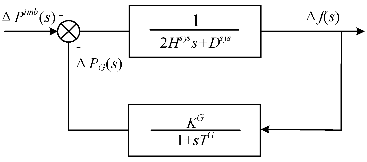
The center-of-inertia frequency response of the power system after a disturbance can be analyzed using the system frequency response model shown in Figure 1. The governor dynamics of diesel generators are modeled as a first-order inertial system [28].
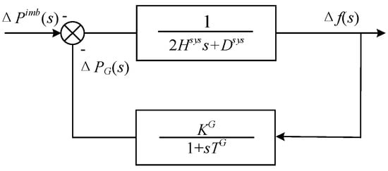
Figure 1.
System frequency response model.
Assuming that a step disturbance occurs, the frequency dynamic process can be expressed as (5).
where:
By performing the inverse Laplace transform on (5), the time-domain expressions for the frequency deviation function in both overdamped and underdamped cases can be obtained. The relevant derivation can be found in [29], where Δfmax is used to represent the expression of MFD. Δf(s), ωn, and ζ represent the frequency deviation, the natural frequency of the system, and the damping ratio, respectively. In (6), Hsys represents the aggregate inertia constant of the microgrid, reflecting the kinetic energy storage capacity; Ksys denotes the system frequency regulation gain, quantifying the primary control response speed; and Dsys models the composite load damping effect, which inherently stabilizes frequency deviations.
2.2. Modeling of Frequency Constraints
2.2.1. RoCoF Constraint
The RoCoF reaches its maximum value immediately after the disturbance and must remain below the permissible threshold:
2.2.2. MFD Constraint
MFD should be constrained to prevent it from exceeding the threshold, which would trigger under-frequency load shedding or over-frequency generator tripping.
The expressions for MFD in both cases are derived (see [29] for the full derivation). The MFD function in the overdamped case is as follows:
where
The MFD function in the underdamped case is as follows:
where
Since the MFD differs between overdamped and underdamped cases, a compact form can be used to represent it:
2.2.3. QSSFD Constraint
The constraint for QSSFD is as follows:
where Δfqss is the calculated quasi-steady-state frequency deviation, and is the maximum allowable quasi-steady-state frequency deviation.
2.3. Modeling of ITAE of Frequency
The calculation of the ITAE of frequency is obtained by integrating |Δf(t)| over time:
Because directly integrating |Δf(t)| is quite challenging, we adopt a more straightforward approach. N points are first uniformly sampled on the frequency response curve within the interval 0–30 s, and then Simpson’s rule is used to compute the integral. Its cubic convergence rate (error ∝ h4) provides superior accuracy compared to the trapezoidal rule for the smooth frequency response curve. Plus, it captures the nonlinear dynamics better than lower-order methods while avoiding Runge–Kutta’s computational overhead.
2.4. Convexification Method for MFD and ITAE of Frequency
ψ1 and ψ2 are denoted as functions of the MFD and ITAE of frequency, respectively. These two functions exhibit highly nonlinear characteristics, making it challenging to embed them into the convex optimization model proposed later. Fortunately, the development of DNNs has made it possible to overcome this difficulty.
DNNs are powerful machine learning models that use multiple layers of neurons to capture complex nonlinear relationships. In DNNs, linear layers can effectively fit highly nonlinear functions, transforming these nonlinear problems into more manageable forms [30].
Training sets are generated within the feasible domain of the features in ψ1 and ψ2, and they are trained separately to predict the MFD and ITAE of frequency. Two linear layers are selected, which already achieve high accuracy. After training, the relationship between the predicted values and the features can be expressed using (15).
The neural network architecture in (15) processes the input through three distinct steps: linear transformation, nonlinear activation, and prediction, where W1 and W2 are the weight matrices for the first and second layers, respectively. b1 and b2 are the bias vectors for the first and second layers, respectively. n is the dimension of the input vector x. In our problem, n = 3, representing the power imbalance, inertia, and damping constants. m is the output dimension of the first linear layer, i.e., the number of neurons in the first linear layer, typically set to 32, 64, or 128. p is the dimension of the final output vector z2. In our problem, p = 1, representing the predicted value of either the MFD or ITAE of frequency. The ReLU activation function is used. The non-convex max(x,y) operator is exactly reformulated as a system of linear inequalities via the big-M method [31].
After training the DNNs, the linearized MFD constraint and ITAE of frequency are reformulated:
3. Formulation of the Proposed Model
3.1. DRFC-ED Scheduling Framework
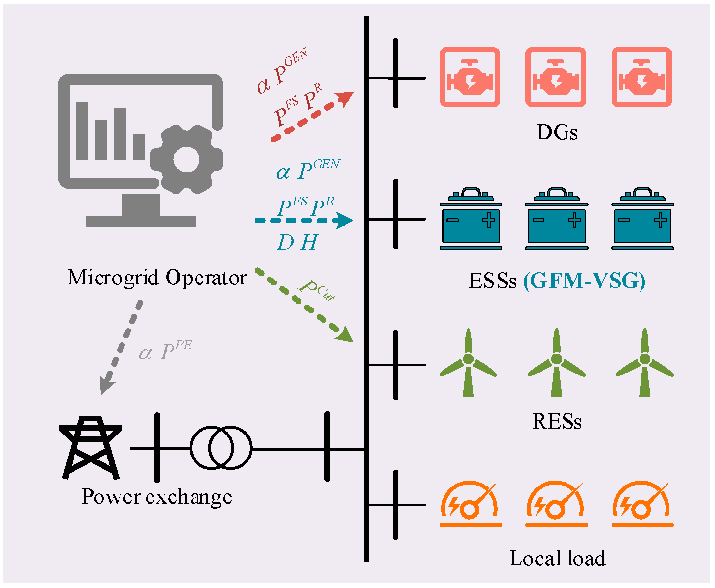
The proposed DRFC-ED scheduling framework is shown in Figure 2. The unit commitment has already been determined in the day-ahead schedule, so the online status of diesel generators is assumed to be already fixed. After each execution of the DRFC-ED, the system operator allocates the optimized inertia and damping constants to each ESS. Additionally, the settings for power and reserves will also be distributed to each device. Considering that excessive reliance on power exchange with the main grid can jeopardize frequency security after unintentional islanding events, certain limits should be placed on the power exchange.
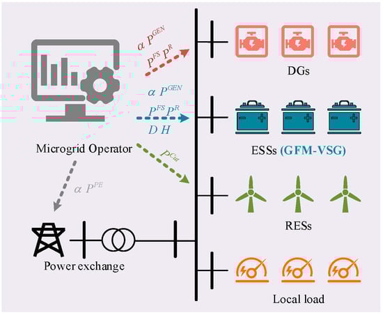
Figure 2.
DRFC-ED scheduling framework.
3.2. Modeling of RESs’ Uncertainty
The actual power of RESs () is composed of the forecasted power () and the forecast error ():
During real-time operation, diesel generators, ESSs, and the power exchange line can adjust their outputs based on an affine strategy [32] to compensate for forecast errors:
3.3. Objective Function
The optimization objectives of DRFC-ED are twofold: minimizing operational costs (F1) and minimizing the ITAE of frequency (F2).
Here, C1–C6 represent the following costs, respectively: fuel cost, regulation reserves cost, PFR reserves cost, power curtailment cost of RESs, power exchange cost, and the expected cost of activating regulation reserves under the worst-case distribution within the ambiguity set of the random variables.
Θ is the set of decision variables:
3.4. Constraints
3.4.1. Power Balance Constraints
The supply and demand balance between generation and consumption should be ensured for each time period:
Expanding (23), we get the following:
It is not difficult to see that when (25) holds, (21) is equivalent to (26). Therefore, (25) and (26) together form the power balance constraint, eliminating the random variables in (24).
3.4.2. Regulation Reserves Constraints
When the participation factor α is not zero, it indicates that certain up/down regulation reserves need to be deployed to cope with the RES fluctuations in real-time operation. Therefore, the following distributionally robust chance constraints apply:
Equation (27) represents that, under the worst-case probability distribution within the ambiguity set of the random variables, the probability that the constraints inside the parentheses are satisfied is at least .
3.4.3. PFR Reserve Constraints
Diesel generators and ESSs need to reserve a certain amount of up and down PFR reserves to handle potential power disturbances:
where γ is the power reserve coefficient, which is set to be 0.5 [10].
3.4.4. Diesel Generator Operation Constraints
The operational constraints for diesel generators include the maximum/minimum power constraints (30) and the ramp-up/ramp-down rate constraints (31).
3.4.5. ESS Operation Constraints
The operational constraints for ESSs are shown in (32)–(36), representing logical constraints between charging/discharging states and positive/negative power, maximum and minimum power constraints, maximum and minimum energy constraints, the energy equality constraint at the beginning and end of the scheduling period, and energy variation constraints.
3.4.6. Power Exchange Line Constraints
The constraints for the power exchange line, as shown in (37), limit its maximum transmission power.
3.4.7. Modeling of Power Disturbances
Power disturbances can be categorized into two types in our model: power fluctuations on the load side and unintentional islanding events. The maximum power imbalance from these two situations is chosen.
where is the load disturbance coefficient.
3.4.8. Frequency Constraints
According to the derivations in Section 2, the constraints for RoCoF, MFD, and QSSFD are shown in (39)–(41), respectively:
where:
The formulation of the DRFC-ED is summarized as follows:
4. Solution Methodology
The proposed DRFC-ED (45) presents several challenging issues that make it unsolvable by off-the-shelf solvers: the expected cost (C6) under the worst-case distribution in the objective function F1, the DR chance constraints in (27), and the two objective functions with different dimensions. Next, the methods to handle each of these issues will be discussed separately.
Before addressing the objective function and DR chance constraints with random variables, the uncertainty of RESs using a Wasserstein distance-based ambiguity set is modeled.
4.1. Modeling of Wasserstein Distance-Based Ambiguity Set
The Wasserstein distance-based ambiguity set is utilized to address uncertainty in the probability distribution of random variables. The modeling process involves the following steps:
4.1.1. Define the Nominal Distribution
Start by specifying the empirical probability distribution , which serves as a reference point. This distribution can be derived from historical data:
where is the Dirac distribution centered on the i-th historical data , and N is the number of historical data.
4.1.2. Define the Wasserstein Distance
The Wasserstein distance quantifies the discrepancy between two probability distributions and . For distributions and , over a metric space (X, d), the Wasserstein distance of order p is defined as follows:
where denotes the set of all couplings of and .
4.1.3. Ambiguity Set Construction
The ambiguity set is constructed using the Wasserstein distance to capture distributions that are close to the empirical distribution . It is defined as follows:
where θ represents the Wasserstein ball radius that quantifies the maximum allowable statistical deviation between the true distribution and the empirical distribution . It is a predefined tolerance level representing the degree of uncertainty, analogous to the radius of a ball around . Therefore, the larger the radius is, the more potential distributions are covered, resulting in greater conservatism.
4.2. Linearization of Objective Function and DR Chance Constraints
Next, the ambiguity set is incorporated into the optimization model. C6 in the objective function F1 and the DR chance constraints (27) in the compact forms can be rewritten as shown in (49) and (50), respectively.
where x is the decision variable, and is a random variable. is the affine objective function (c is the deterministic cost vector, d is the uncertainty penalty weights). is the constraint sensitivity vector (A: linear coefficient matrix, α: intercept term). is the constraint threshold function (B: linear coefficients, β: safety margin).
According to [22], the expected cost under the worst-case distribution based on the Wasserstein distance-based ambiguity set (49) can be transformed into the following linear program:
where χ is a dual multiplier. The non-convex DR chance constraint (51) can be approximated by the conditional value at risk (CVaR) constraint. Finally, the CVaR constraint is transformed into the following linear program:
where and are dual multipliers and is an auxiliary variable [22].
Thus, the non-convex terms of (49) and (50) are transformed into the linear programs of (51) and (52), respectively.
4.3. Solution Method for the DRFC-ED
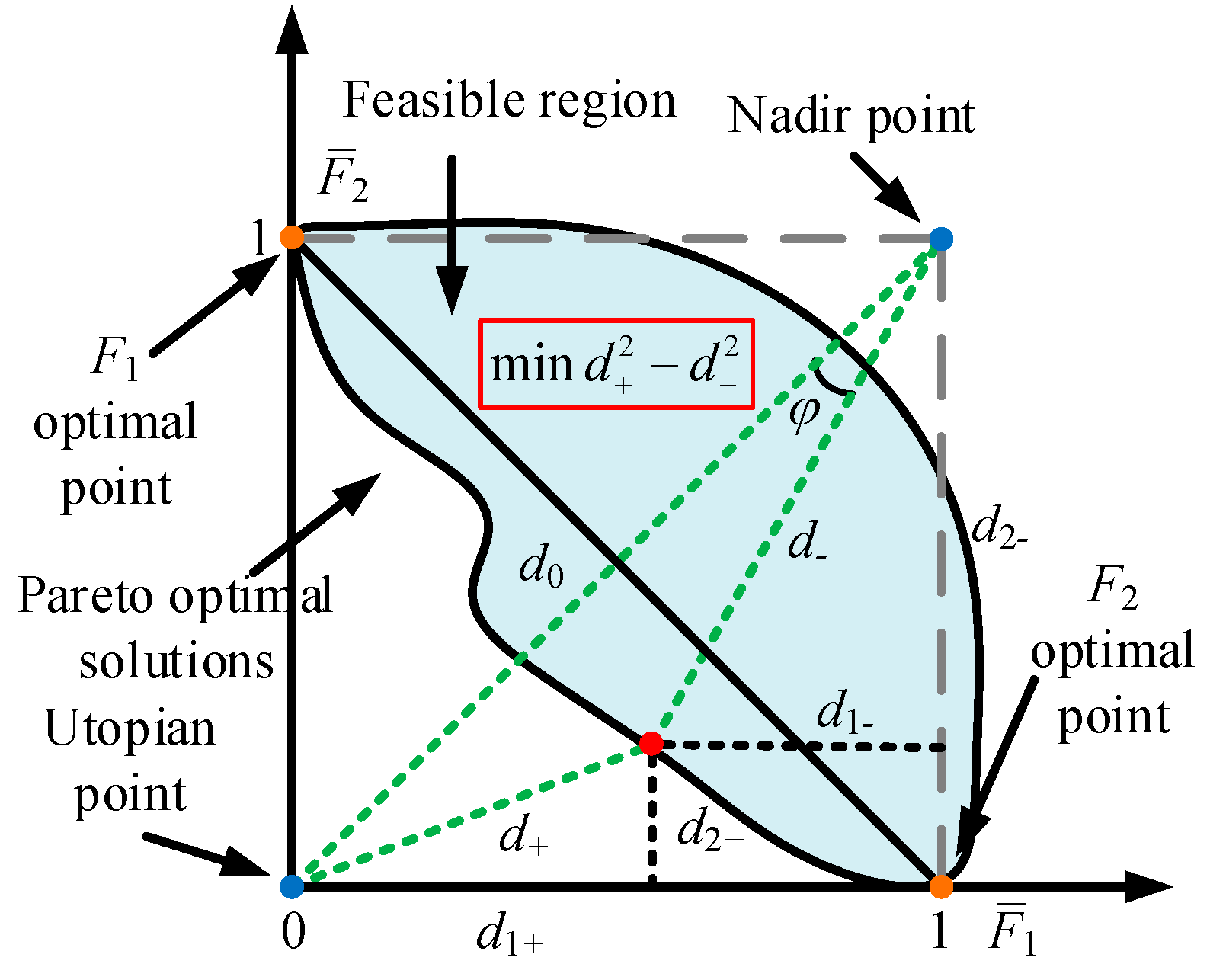
For the DRFC-ED model, increasing the virtual inertia or damping can obviously improve the ITAE of frequency, but it also increases the reserves required from ESSs, limiting their charging and discharging power and thus reducing economic efficiency. Therefore, the two objectives not only have different dimensions but are also counterbalancing each other. Traditionally, solving a multi-objective optimization model involves finding all non-dominated solutions to form the Pareto optimal solutions [33]. Then, a compromise optimal solution is selected from the Pareto optimal solutions as the optimal decision. However, obtaining Pareto optimal solutions requires extensive computation time. To improve computational efficiency, the aim is to minimize the difference between the distance of the compromise solution to the utopian point and to the nadir point [34]. This approach does not require solving for all non-dominated solutions, allowing us to directly search within the feasible region for the compromise solution that is closest to the utopian solution.
Figure 3 illustrates the principle of the directly obtained compromise optimal solution method. First, solve the single-objective optimization model for each objective Fi(x) to obtain the optimal solutions xi* (i = 1, 2). This process also determines the utopian point (F1(x1*), F2(x2*)), the payoff matrix (49), and the maximum values of each objective Fi,max in the matrix, leading to the identification of the nadir point (F1,max, F2,max). Then, by minimizing the difference between the squared distance to the utopian point (d+) and the squared distance to the nadir point (d−), the multi-objective problem can be transformed into a single-objective problem, as shown in (54), where Δd2 is the quadratic difference between d+ and d−. A smaller Δd2 reflects a closer approximation to the utopian point, representing a better trade-off among conflicting objectives.

Figure 3.
The principle of the directly obtained compromise optimal solution.
For the transformation from to , please refer to [29].
5. Case Study
The effectiveness of the proposed DRFC-ED is evaluated using a test microgrid system composed of four diesel generators, four ESSs, one wind turbine, one photovoltaic generator, and one aggregate load. The case study is carried out on a computer with a 3.00 GHz Intel Core i5-8500 CPU and 16 GB of RAM, using Gurobi 11.0.0 as the solver and Python 3.10.6 as the programming language.
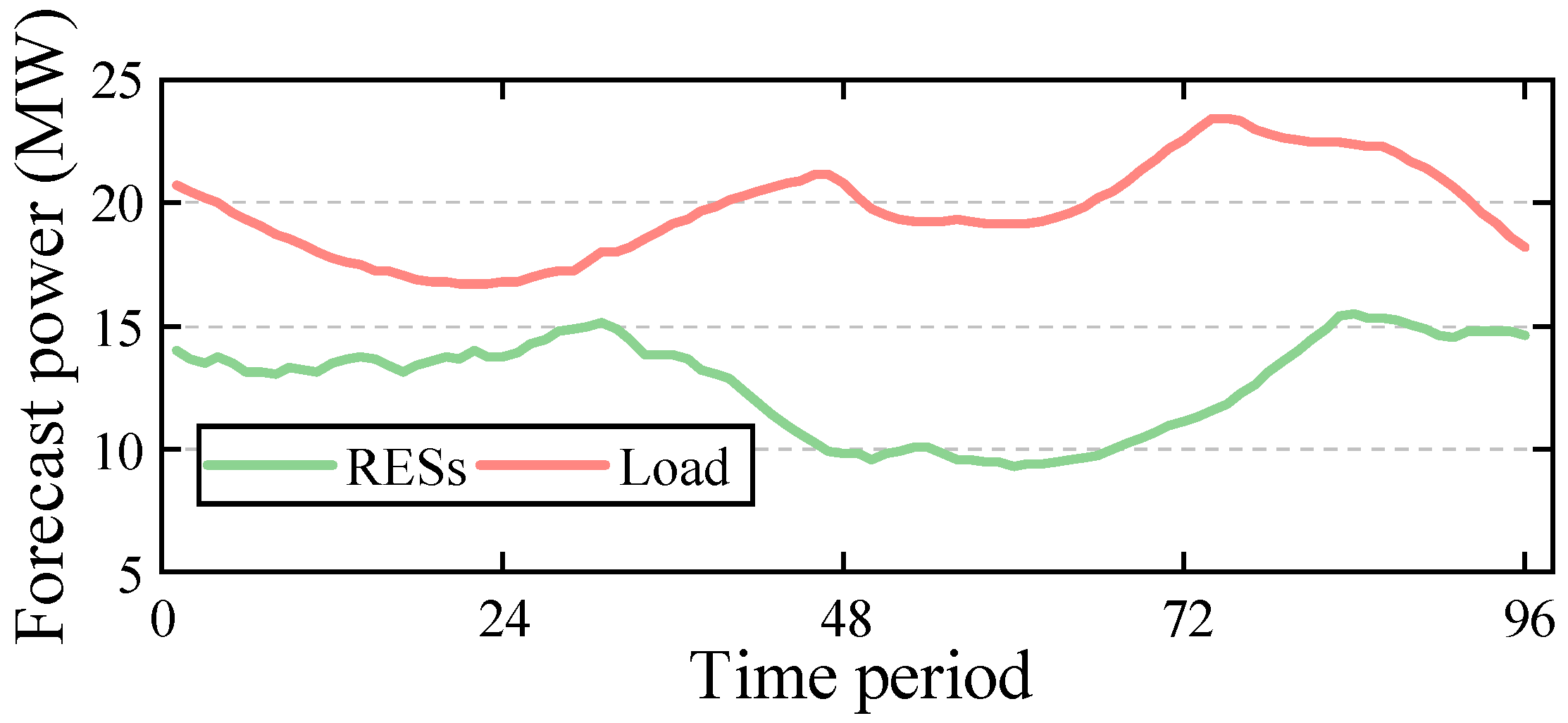
The forecast power for the RESs and load are scaled based on actual data from a region in Guangdong Province, China, as shown in Figure 4. Data for the diesel generators, ESSs, and power prices have been uploaded to [29].
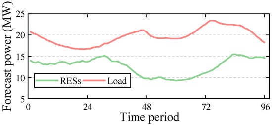
Figure 4.
Forecast power of RESs and load.
Based on the RES forecast value, 5000 samples conforming to a normal distribution with a mean of 0 and a standard deviation of 15% of the forecast value are generated using the Monte Carlo sampling method. From these samples, 20 samples are selected to construct the ambiguity set. The remaining samples are used to verify the empirical violation probability (EVP) of each chance constraint, with a confidence level of = 95%.
The power base value PB is 100 MW, and the nominal frequency is 50 Hz. The frequency constraint limits , , and are set to 1 Hz/s, 0.5 Hz, and 0.25 Hz, respectively. The load damping coefficient DL is 0 [35]. The load disturbance coefficient = 15%. Additionally, before training the DNNs, the number of neurons is set to 32 for each layer, i.e., m = 32. The mean squared error is chosen as the loss function, and the maximum number of epochs is set to 1000. The ITAE of frequency is calculated by integrating the frequency deviation, with an integration step size of 0.01 s and an integration time of 30 s.
To facilitate subsequent explanations, the following three models are defined: M1—a DR-ED model for microgrids without considering frequency constraints and the ITAE of frequency; M2—a single-objective DRFC-ED model considering frequency constraints but not the ITAE of frequency; and M3—the proposed multi-objective DRFC-ED model.
5.1. Selection of Ball Radius θ
Before performing multi-objective optimization, it is necessary to calculate the optimal and worst values for each single-objective problem. Different radii result in varying degrees of conservative estimation of the RESs’ uncertainty, thereby affecting the upper and lower bounds of objective F1. Therefore, the M2 model under different ball radius settings to obtain a trade-off between EVP and economic performance is first solved. Based on this, the M3 model is then solved.
The M2 model under five different ball radius settings is solved, and the results are shown in Table 2. As can be seen, when the ball radius is equal to 0.025 and 0.02, the maximum EVP among all DR chance constraints exceeds 5%, failing to meet the set confidence level. When the ball radius is greater than or equal to 0.03, the maximum EVP meets the requirement, albeit at the cost of increased economic expense. Balancing the maximum EVP and economic efficiency, θ = 0.03 is chosen as a compromise.
Table 2.
Results under different ball radii.
It should be noted that once the ball radius is determined, the maximum EVP in the M1–M3 models will be the same. Therefore, it is a reasonable practice to first determine the ball radius through M2.
5.2. Comparison of Optimization Results
5.2.1. Comparison of Single-Objective and Multi-Objective Optimization Results
After determining the ball radius, the DRFC-ED is solved with F1 from (20) and F2 from (21) as the optimization objectives, respectively, to obtain the optimal and worst values of each objective. Subsequently, M3 is solved. The results of the single-objective and multi-objective optimization models are shown in Table 3.
Table 3.
Results of single-objective and multi-objective models.
It can be seen that when F1 is the objective, the model is economically optimal but overlooks the ITAE of frequency. When F2 is the objective, the model fully deploys the inertia and damping of ESSs, increasing the reserve costs of ESSs and thereby increasing economic costs. However, in the multi-objective optimization model, by directly solving for the compromise optimal solution, the ITAE of frequency improves by 8.03% at the cost of only a 2.1% increase in economic costs. This demonstrates that the proposed multi-objective formulation enables a balance between economic efficiency and frequency performance.
5.2.2. Optimization Results of M1–M3
Table 4 presents the optimization results of M1–M3. From the perspective of economic costs, the costs for M2 and M3 are approximately 37% higher than those for M1. This is because M2 and M3 incur additional PFR reserve costs due to the inclusion of frequency constraints. Additionally, more power is sourced from diesel generators and ESSs rather than the main grid to prevent excessive power imbalance after unintentional islanding events, resulting in higher power exchange costs for M1 compared to M2 and M3.
Table 4.
Optimization results of M1–M3.
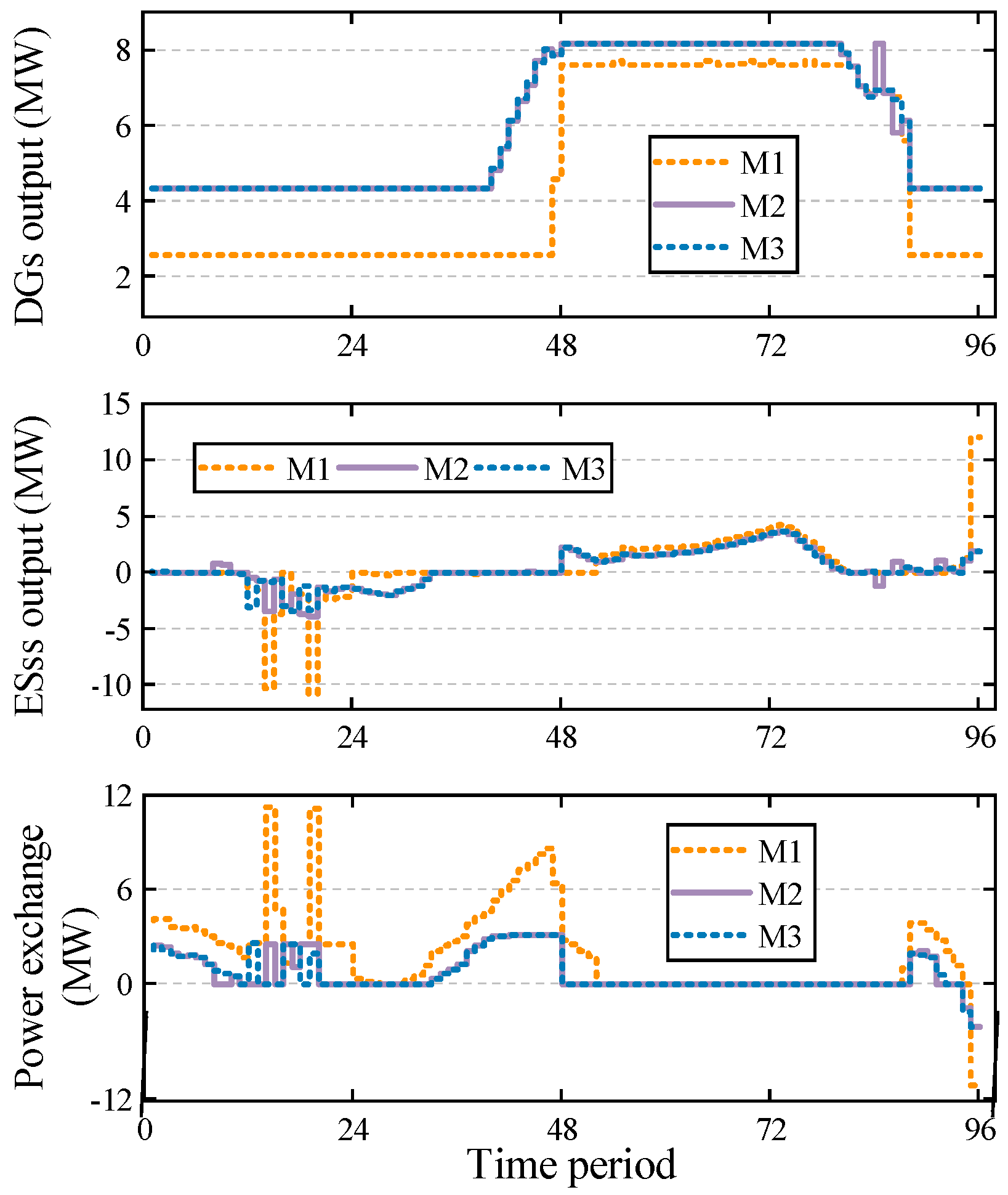
Figure 5 shows the scheduling results of diesel generators, ESSs, and power exchange for the three models. It can be observed that due to the lack of frequency constraints, M1 purchases a large amount of power from the main grid at night and stores it in ESSs, which then supply power during the day when the RES output is low. This results in lower power supply requirements from diesel generators compared to M2 and M3. However, under such a scheduling result, unintentional islanding events would result in a significant power imbalance, posing safety risks. After considering frequency constraints, M2 and M3 both limit power exchange and rely more on power generation from devices within the microgrid to ensure frequency security after unintentional islanding events.
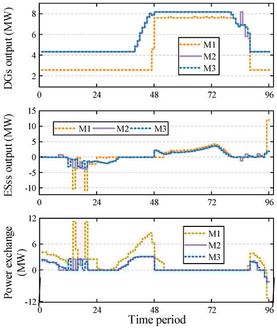
Figure 5.
The scheduling results of diesel generators (DGs) (top), ESSs (middle), and power exchange (bottom) for M1–M3.
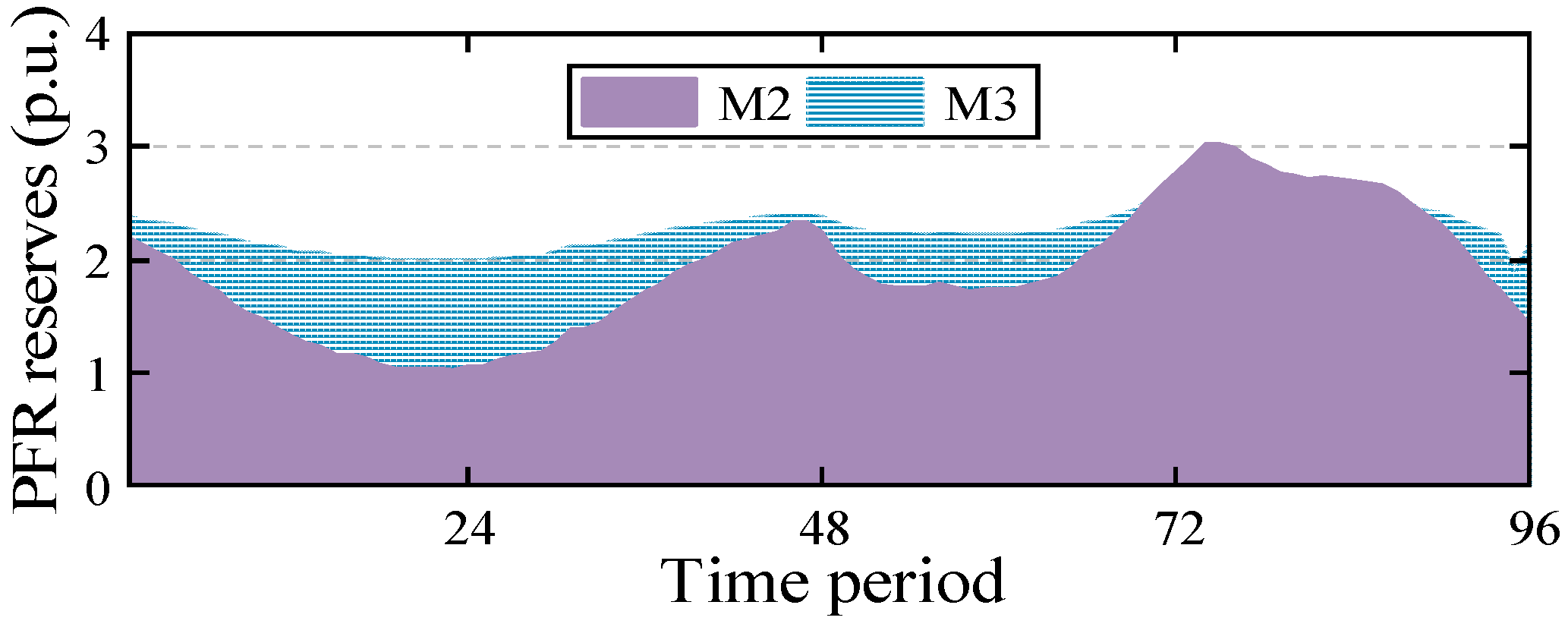
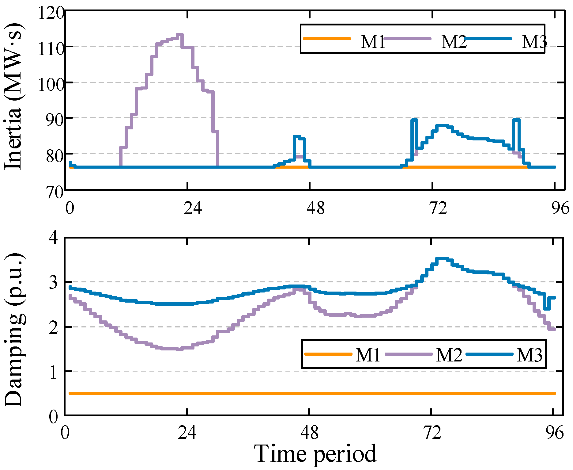
Comparing M2 and M3, the most significant difference lies in the PFR reserve costs (the PFR reserve scheduling results are shown in Figure 6). Since M3 optimizes the ITAE of frequency, it results in more damping being deployed (damping is more effective than inertia in improving the ITAE of frequency [18]). M2, on the other hand, only ensures that the frequency constraints are met without considering the different characteristics of inertia and damping in the frequency response. Figure 7 shows the scheduling results of the ESSs’ virtual inertia and damping in M2 and M3. The orange line serves as a baseline, representing the inherent inertia and damping of diesel generators. It can be observed that M2 prioritizes the deployment of the ESSs’ inertia because this approach maximizes benefits while ensuring frequency security. In contrast, M3 prioritizes the deployment of damping to optimize the ITAE of frequency, which leads to a reduction in inertia deployment to keep the ESSs’ PFR reserve costs from being excessively high. Furthermore, Figure 8 shows the scheduling results for each ESS’s virtual inertia and damping in M3. It can be observed that only the inertia of ESS #1 is deployed, while the inertias of ESSs #2–#4 are not scheduled. In terms of damping scheduling, the damping for ESSs #1 and #2 is fully deployed to the maximum limit, while ESS #3 reaches full deployment in some cases, and ESS #4 is scheduled the least. This is because the PFR reserve cost coefficients increase from ESS #1 to ESS #4, leading to the prioritization of the more cost-effective ESS #1 for inertia and damping scheduling.
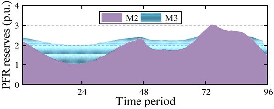
Figure 6.
The scheduling results of PFR reserves for M2–M3.
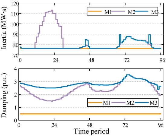
Figure 7.
The scheduling results of ESSs’ virtual inertia (top) and damping (bottom) for M2–M3.
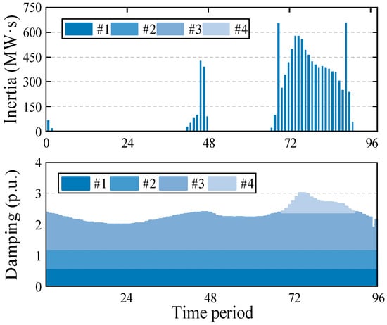
Figure 8.
The scheduling results for each ESS’s virtual inertia (top) and damping (bottom) in M3.
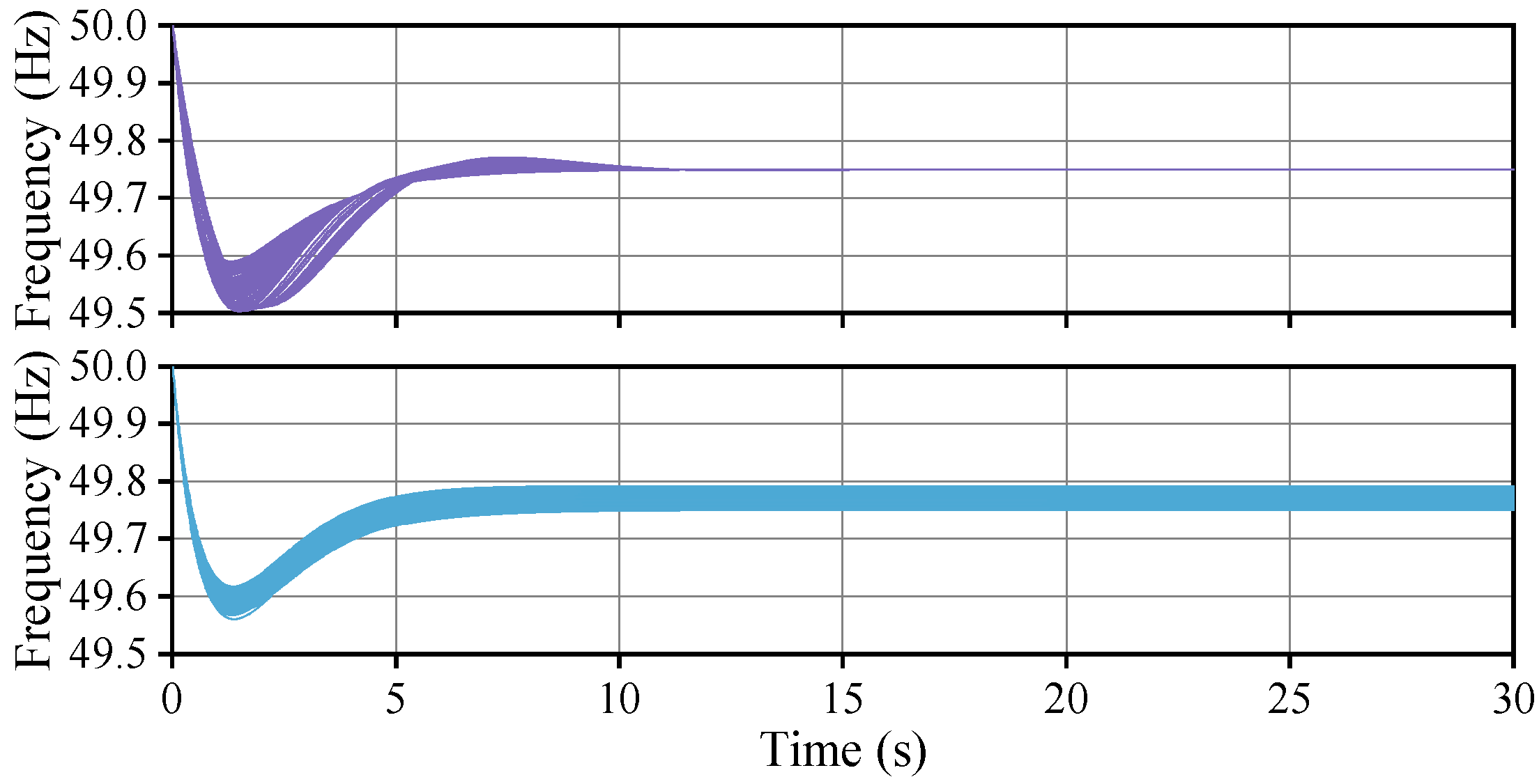
By inputting the scheduling results of each time period for M2 and M3 into the system frequency response model, we obtain the frequency response curves for M2 and M3 (calculated for low-frequency scenarios), as shown in Figure 9. It can be seen that M3, which schedules more virtual damping, has a smaller QSSFD compared to M2. Additionally, the distribution range of QSSFD for M3 is broader, while M2 maintains the QSSFD at 0.25 Hz, which is the set threshold. Furthermore, M3 shows no oscillation process before reaching quasi-steady-state, indicating better stability. In contrast, M2’s frequency curve is not smooth due to lower damping. This phenomenon supports the conclusion of Sajadi et al. that increasing damping can alleviate concerns among power system experts regarding the reduction of inertia [18].
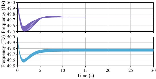
Figure 9.
Frequency response of M2 (purple) and M3 (blue).
5.2.3. Verification of Frequency Constraints’ Effectiveness
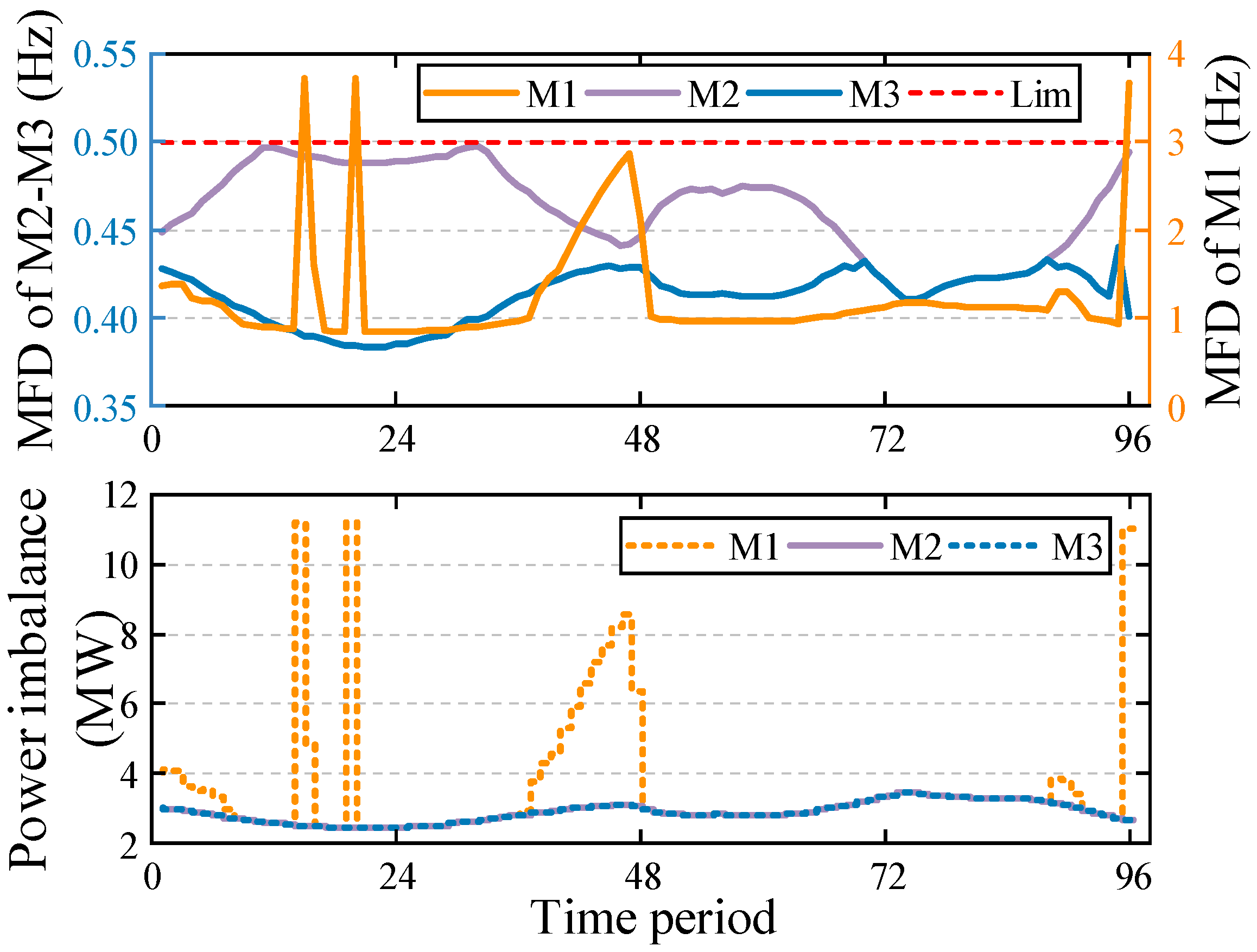
Figure 10 shows the MFD and the maximum power imbalance of M1–M3. Since the RoCoF constraint and the QSSFD constraint are linear constraints and do not involve errors, their results are not displayed here. It can be observed that, due to the lack of constraints on power exchange in M1, the power exchange line transmits a large capacity during nighttime. If unintentional islanding events occur at this time, the MFD can reach 3.5 Hz, severely impacting power supply reliability.

Figure 10.
MFD (top) and power imbalance (bottom) of M1–M3.
In contrast, M2 and M3, after applying frequency constraints, strictly maintain the MFD within 0.5 Hz and also impose limits on power exchange. The maximum power imbalance in all cases is kept below 15% of the current load power. This ensures that seamless islanding can be maintained after unintentional islanding events, and frequency support capability is available during load disturbances.
Additionally, it can be observed that although the MFD of both M2 and M3 remains below 0.5 Hz, M3 is farther away from the threshold. Therefore, the improvement in the ITAE of frequency is closely related to the frequency metrics.
5.2.4. Verification of the Effectiveness of DNN Method
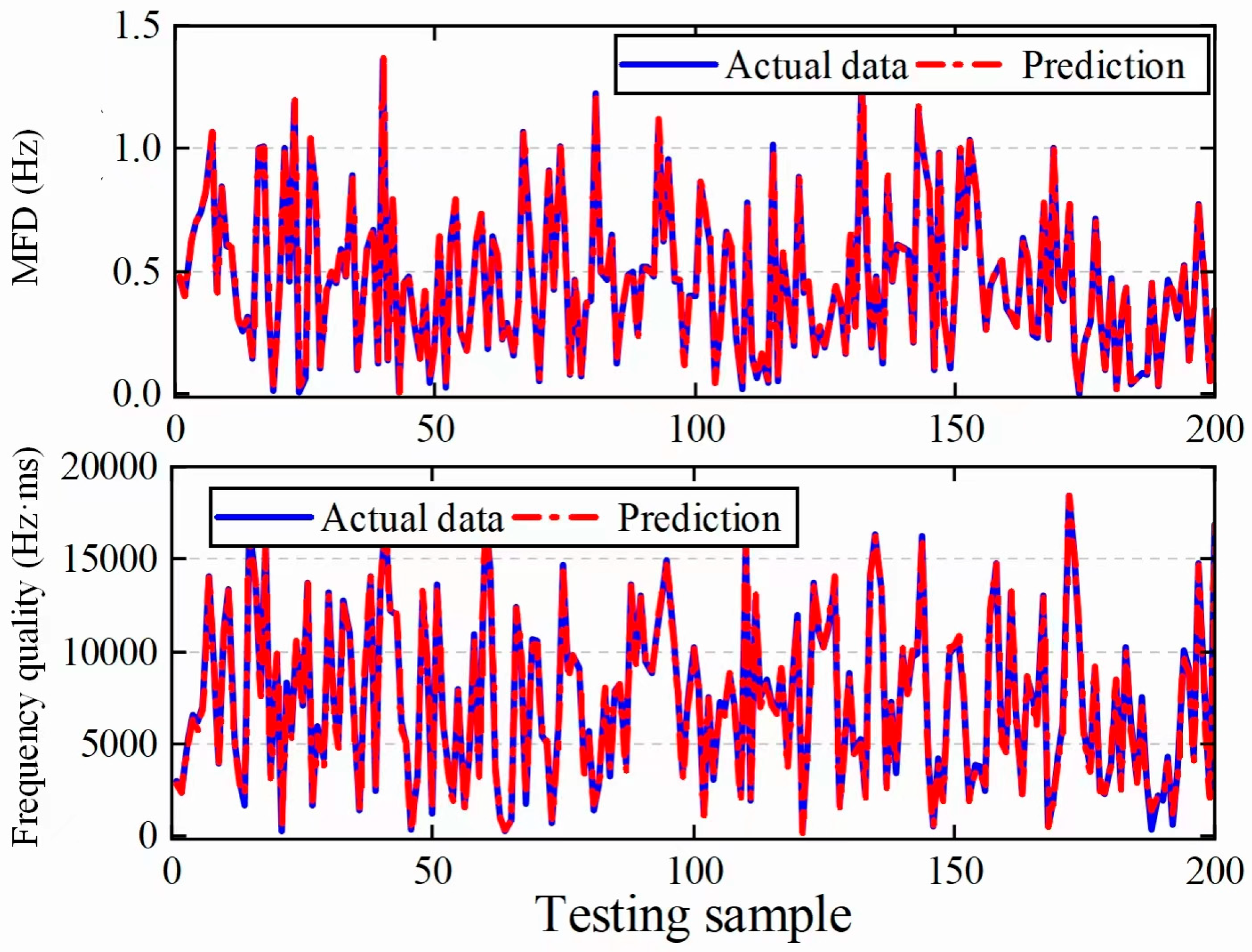
The Latin Hypercube Sampling method is used to sample power imbalance, inertia, and damping constants, generating 20,000 samples. Of these, 90% are used for training the DNNs, while 10% are used for testing. Table 5 presents the evaluation metrics of the DNNs used for convexifying the MFD constraint (DNN1) and frequency quality (DNN2). Figure 11 shows the testing performance of DNN1 and DNN2 based on 200 samples drawn from 2000 testing samples.
Table 5.
Evaluation metrics of DNN1 and DNN2.
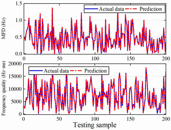
Figure 11.
Testing result of DNN1 (top) and DNN2 (bottom).
It can be observed that the DNN method shows high accuracy in convexifying the MFD constraint and frequency quality. Additionally, the inclusion of DNNs does not introduce excessive computational burden. The average time to solve M3 is only 8 s with a convergence gap of 0.1%.
Additionally, we compared the predicted values at each time period in M3 with the actual values obtained through simulation by substituting the solved results. The relative error statistics are shown in Table 6. It can be observed that the performance of the DNNs is satisfactory when applied to the DRFC-LAED.
Table 6.
Relative error statistics.
5.2.5. Comparison of Different Stochastic Optimization Methods
The optimization results and maximum EVP of M2 under different stochastic optimization methods are compared. The definitions are as follows: C1—Gaussian-approximation chance-constrained method, where the uncertainty of RESs is assumed to follow a Gaussian distribution; C2—moment-based ambiguity set DRCC method; and C3—Wasserstein distance-based ambiguity set DRCC method (θ = 0.03).
Table 7 presents the results under different stochastic optimization methods. It can be observed that the cost of C1 is lower than that of C2 and C3, but the maximum EVP exceeds the set threshold. This approach, which directly assumes a Gaussian distribution for the RESs’ uncertainty, clearly fails to meet the requirements. Both C2 and C3 satisfy the confidence level constraint, but the cost of C2 is higher than C3, despite its maximum EVP being well below 5%. This is because the moment-based ambiguity set can only utilize the mean and variance of historical data. In contrast, the Wasserstein distance-based ambiguity set can more comprehensively utilize the available data. Therefore, its conservativeness is reduced, but it can still balance conservativeness by controlling the ball radius.
Table 7.
Results under different stochastic optimization methods.
6. Conclusions
This paper proposes a microgrid frequency response enhancement-oriented DRFC-ED dispatch model. For the first time, the ITAE of frequency is used as a metric to optimally deploy the combination of system inertia and damping in frequency-constrained optimal dispatch research while also optimizing the coordination of diesel generators, ESSs, RESs, and power exchange. The case study verifies that the DRFC-ED model can effectively ensure frequency security at the system operation level. Furthermore, case studies confirm that the damping coefficients exhibit greater sensitivity in minimizing the ITAE metric compared to inertia constants. Strategic damping enhancement can alleviate concerns about the reduction of inertia. The proposed DNN-based convexification method achieves satisfactory accuracy. Additionally, the proposed method effectively solves the multi-objective optimization problem without incurring extra computational burden. The uncertainty of RESs is effectively managed through the distributionally robust chance-constrained approach, which ensures that the EVP does not exceed the limit. This study contributes to enhancing both the economic efficiency and dynamic security in renewable-dominated microgrids while addressing critical challenges in modern power systems.
While this study focuses on inertia-damping coordination via ITAE optimization, two important extensions are warranted: (1) incorporating RES frequency support mechanisms (e.g., wind turbine virtual inertia and PV droop control) to enhance primary frequency response, and (2) exploring hybrid ambiguity sets (e.g., Wasserstein-moment combined) for uncertainty modeling to balance the robustness and computational efficiency. These directions will be pursued in subsequent research.
Author Contributions
Methodology, D.X. and L.G.; Formal analysis, Z.W.; Data curation, C.C.; Writing—original draft, C.C.; Writing—review & editing, D.X. All authors have read and agreed to the published version of the manuscript.
Funding
This work is supported by the National Natural Science Foundation of China (U22B6007).
Data Availability Statement
The original data presented in the study are openly available at https://www.jianguoyun.com/p/DTJKXycQko_hChj7p-EFIAA, accessed on 9 April 2025.
Conflicts of Interest
The authors declare no conflicts of interest. The funders had no role in the design of the study; in the collection, analyses, or interpretation of data; in the writing of the manuscript; or in the decision to publish the results.
Abbreviations
The following abbreviations are used in this manuscript:
| RESs | Renewable energy sources |
| DRFC-ED | Distributionally robust frequency-constrained economic dispatch |
| MFD | Maximum frequency deviation |
| ITAE | Integral time absolute error |
| ESSs | Energy storage systems |
| PFR | Primary frequency response |
| RoCoF | Rate of change of frequency |
| QSSFD | Quasi-steady-state frequency deviation |
Nomenclature
| Indices and Sets | |
| g/G, r/R, e/E, d/D, t/T | Index and set of diesel generators, renewable energy sources (RESs) generators, energy storage systems (ESSs), local loads, time periods |
| Parameters | |
| Hsys | System inertia constant |
| Dsys | System damping constant |
| KG | Droop coefficient of aggregated diesel generators |
| TG | Governor constant of aggregated diesel generators |
| f0 | Nominal frequency |
| ag/bg/cg | Fuel cost coefficients of diesel generators |
| // | Regulation reserve cost coefficients of diesel generators, ESS and power exchange line |
| / | Primary frequency response (PFR) reserve cost coefficients of diesel generators and ESS |
| Power curtailment cost coefficient of RES | |
| / | Regulation reserve activation cost coefficients of diesel generators, ESS, and power exchange line |
| // | Regulation reserve activation cost coefficients of diesel generators, ESS, and power exchange line |
| // | Output upper limit of diesel generators, ESS, and power exchange line |
| / | Upward and downward ramp limit of diesel generators |
| M | A big positive number |
| / | Energy capacity and state of charge upper limit of ESS |
| ηe | Charge and discharge efficiency coefficient of ESS |
| Δtp | Charge and discharge time of ESS |
| Pd,t | Local load power at time t |
| Variables | |
| αg,t/αe,t/ | Participation factor of diesel generators, ESS, and power exchange line at time t |
| ϑt | Power exchange direction: 1 indicates injection into microgrids at time t |
| // | Output of diesel generators, RES, and ESS at time t |
| / | Inertia and damping constants of ESS at time t |
| Power exchange at time t | |
| / | Auxiliary variable and power imbalance at time t |
| Power curtailment of RES at time t | |
| SOCe,t | State of charge of ESS at time t |
| / | Charge and discharge state of ESS at time t |
| // | Upward regulation reserves of diesel generators, ESS, and power exchange line at time t |
| // | Downward regulation reserves of diesel generators, ESS, and power exchange line at time t |
| / | Upward PFR reserves of diesel generators and ESS at time t |
| / | Downward PFR reserves of diesel generators and ESS at time t |
References
- Hirsch, A.; Parag, Y.; Guerrero, J. Microgrids: A review of technologies, key drivers, and outstanding issues. Renew. Sustain. Energy Rev. 2018, 90, 402–411. [Google Scholar] [CrossRef]
- Zhang, Y.; Chen, C.; Liu, G.; Hong, T.; Qiu, F. Approximating Trajectory Constraints with Machine Learning—Microgrid Islanding with Frequency Constraints. IEEE Trans. Power Syst. 2021, 36, 1239–1249. [Google Scholar] [CrossRef]
- Chan, M.L.; Dunlop, R.D.; Schweppe, F. Dynamic Equivalents for Average System Frequency Behavior Following Major Distribances. IEEE Trans. Power Appar. Syst. 1972, PAS-91, 1637–1642. [Google Scholar] [CrossRef]
- Shi, Q.; Li, F.; Cui, H. Analytical Method to Aggregate Multi-Machine SFR Model with Applications in Power System Dynamic Studies. IEEE Trans. Power Syst. 2018, 33, 6355–6367. [Google Scholar] [CrossRef]
- Badesa, L.; Teng, F.; Strbac, G. Optimal Portfolio of Distinct Frequency Response Services in Low-Inertia Systems. IEEE Trans. Power Syst. 2020, 35, 4459–4469. [Google Scholar] [CrossRef]
- Xu, D.; Wu, Z. Enhanced frequency aware microgrid scheduling towards seamless islanding under frequency support of heterogeneous resources: A distributionally robust chance constrained approach. Int. J. Electr. Power Energy Syst. 2024, 162, 110310. [Google Scholar] [CrossRef]
- Lagos, D.T.; Hatziargyriou, N.D. Data-Driven Frequency Dynamic Unit Commitment for Island Systems with High RES Penetration. IEEE Trans. Power Syst. 2021, 36, 4699–4711. [Google Scholar] [CrossRef]
- Xu, D.; Wu, Z.; Zhu, L.; Guan, L. A novel frequency constrained unit commitment considering VSC-HVDC’s frequency support in asynchronous interconnected system under renewable energy Source’s uncertainty. Electr. Power Syst. Res. 2025, 238, 111098. [Google Scholar] [CrossRef]
- Xu, D.; Wu, Z.; Liu, Y.; Zhu, L. Enhancing frequency security for renewable-dominated power systems via distributionally robust frequency constrained unit commitment. Electr. Power Syst. Res. 2025, 239, 111078. [Google Scholar] [CrossRef]
- Zhang, Z.; Du, E.; Teng, F.; Zhang, N.; Kang, C. Modeling Frequency Dynamics in Unit Commitment with a High Share of Renewable Energy. IEEE Trans. Power Syst. 2020, 35, 4383–4395. [Google Scholar] [CrossRef]
- Shen, Y.; Wu, W.; Wang, B.; Sun, S. Optimal Allocation of Virtual Inertia and Droop Control for Renewable Energy in Stochastic Look-Ahead Power Dispatch. IEEE Trans. Sustain. Energy 2023, 14, 1881–1894. [Google Scholar] [CrossRef]
- Liang, Z.; Chung, C.Y.; Zhang, W.; Wang, Q.; Lin, W.; Wang, C. Enabling high-efficiency economic dispatch of hybrid AC/DC networked microgrids: Steady-state convex bi-directional converter models. IEEE Trans. Smart Grid 2024, 16, 45–61. [Google Scholar] [CrossRef]
- Shen, Z.; Zhu, J.; Ge, L.; Bu, S.; Zhao, J.; Chung, C.Y.; Li, X.; Wang, C. Variable-Inertia Emulation Control Scheme for VSC-HVDC Transmission Systems. IEEE Trans. Power Syst. 2022, 37, 629–639. [Google Scholar] [CrossRef]
- Jiang, B.; Guo, C.; Chen, Z. Modeling the Coupling of Rotor Speed, Primary Frequency Reserve and Virtual Inertia of Wind Turbines in Frequency Constrained Look-Ahead Dispatch. IEEE Trans. Sustain. Energy 2024, 15, 1885–1899. [Google Scholar] [CrossRef]
- International Renewable Energy Agency. Grid Codes for Renewable Powered Systems. 2022. Available online: https://www.irena.org/-/media/Files/IRENA/Agency/Publication/2022/Apr/IRENA_Grid_Codes_Renewable_Systems_2022.pdf (accessed on 9 April 2025).
- Li, J.; Qiao, Y.; Lu, Z.; Ma, W.; Cao, X.; Sun, R. Integrated Frequency-constrained Scheduling Considering Coordination of Frequency Regulation Capabilities from Multi-Source Converters. J. Mod. Power Syst. Clean Energy 2024, 12, 261–274. [Google Scholar] [CrossRef]
- Yang, Y.; Peng, J.C.-H.; Ye, C.; Ye, Z.-S. Optimal Reserve Allocation with Simulation-Driven Frequency Dynamic Constraint: A Distributionally Robust Approach. IEEE Trans. Circuits Syst. II Express Briefs 2022, 69, 4483–4487. [Google Scholar] [CrossRef]
- Sajadi, A.; Kenyon, R.W.; Hodge, B.-M. Synchronization in electric power networks with inherent heterogeneity up to 100% inverter-based renewable generation. Nat. Commun. 2022, 13, 2490. [Google Scholar] [CrossRef]
- Mohamed, M.M.; El Zoghby, H.M.; Sharaf, S.M.; Mosa, M.A. Optimal virtual synchronous generator control of battery/supercapacitor hybrid energy storage system for frequency response enhancement of photovoltaic/diesel microgrid. J. Energy Storage 2022, 51, 104317. [Google Scholar] [CrossRef]
- Delkhosh, H.; Seifi, H. Power System Frequency Security Index Considering All Aspects of Frequency Profile. IEEE Trans. Power Syst. 2021, 36, 1656–1659. [Google Scholar] [CrossRef]
- Bonnett, A.H. The impact that voltage and frequency variations have on AC induction motor performance and life in accordance with NEMA MG-1 standards. In Proceedings of the Conference Record of 1999 Annual Pulp and Paper Industry Technical Conference (Cat. No. 99CH36338), Seattle, WA, USA, 21–25 June 1999; pp. 16–26. [Google Scholar] [CrossRef]
- Mohajerin Esfahani, P.; Kuhn, D. Data-driven distributionally robust optimization using the Wasserstein metric: Performance guarantees and tractable reformulations. Math. Program. 2018, 171, 115–166. [Google Scholar] [CrossRef]
- Yang, L.; Xu, Y.; Zhou, J.; Sun, H. Distributionally Robust Frequency Constrained Scheduling for an Integrated Electricity-Gas System. IEEE Trans. Smart Grid 2022, 13, 2730–2743. [Google Scholar] [CrossRef]
- Chu, Z.; Zhang, N.; Teng, F. Frequency-Constrained Resilient Scheduling of Microgrid: A Distributionally Robust Approach. IEEE Trans. Smart Grid 2021, 12, 4914–4925. [Google Scholar] [CrossRef]
- Zhou, J.; Guo, Y.; Yang, L.; Shi, J.; Zhang, Y.; Li, Y.; Guo, Q.; Sun, H. A review on frequency management for low-inertia power systems: From inertia and fast frequency response perspectives. Electr. Power Syst. Res. 2024, 228, 110095. [Google Scholar] [CrossRef]
- Zhang, J. Droop coefficient placements for grid-side energy storage considering nodal frequency constraints under large disturbances. Appl. Energy 2024, 357, 122444. [Google Scholar] [CrossRef]
- Peng, Q.; Yang, Y.; Liu, T.; Blaabjerg, F. Coordination of Virtual Inertia Control and Frequency Damping in PV Systems for Optimal Frequency Support. CPSS Trans. Power Electron. Appl. 2020, 5, 305–316. [Google Scholar] [CrossRef]
- Zhang, Y.; Wu, S.; Lin, J.; Wu, Q.; Shen, C.; Liu, F. Frequency Reserve Allocation of Large-Scale RES Considering Decision-Dependent Uncertainties. IEEE Trans. Sustain. Energy 2024, 15, 339–354. [Google Scholar] [CrossRef]
- Wu, Z. Supplemental Material of DRFC-ED. 2024. Available online: https://www.jianguoyun.com/p/DTJKXycQko_hChj7p-EFIAA (accessed on 9 April 2025).
- Zhang, Y.; Cui, H.; Liu, J.; Qiu, F.; Hong, T.; Yao, R.; Li, F. Encoding Frequency Constraints in Preventive Unit Commitment Using Deep Learning with Region-of-Interest Active Sampling. IEEE Trans. Power Syst. 2022, 37, 1942–1955. [Google Scholar] [CrossRef]
- She, B.; Li, F.; Cui, H.; Wang, J.; Zhang, Q.; Bo, R. Virtual Inertia Scheduling (VIS) for Real-Time Economic Dispatch of IBR-Penetrated Power Systems. IEEE Trans. Sustain. Energy 2024, 15, 938–951. [Google Scholar] [CrossRef]
- Zhang, Y.; Shen, S.; Mathieu, J.L. Distributionally Robust Chance-Constrained Optimal Power Flow with Uncertain Renewables and Uncertain Reserves Provided by Loads. IEEE Trans. Power Syst. 2017, 32, 1378–1388. [Google Scholar] [CrossRef]
- Liang, W.; Lin, S.; Liu, J.; Dong, P.; Liu, M. Multi-Objective Mixed-Integer Convex Programming Method for the Siting and Sizing of UPFCs in a Large-Scale AC/DC Transmission System. IEEE Trans. Power Syst. 2023, 38, 5671–5686. [Google Scholar] [CrossRef]
- Liang, Y.; Lin, S.; Feng, X.; Lai, X.; Liu, M. Multi-objective Optimal Planning for AC Electrical Collector and VSC-MTDC Transmission. Power Syst. Technol. 2023, 48, 2404–2415. [Google Scholar] [CrossRef]
- Yang, L.; Li, H.; Zhang, H.; Wu, Q.; Cao, X. Stochastic-Distributionally Robust Frequency-Constrained Optimal Planning for an Isolated Microgrid. IEEE Trans. Sustain. Energy. 2024, 15, 2155–2169. [Google Scholar] [CrossRef]

Disclaimer/Publisher’s Note: The statements, opinions and data contained in all publications are solely those of the individual author(s) and contributor(s) and not of MDPI and/or the editor(s). MDPI and/or the editor(s) disclaim responsibility for any injury to people or property resulting from any ideas, methods, instructions or products referred to in the content. |
© 2025 by the authors. Licensee MDPI, Basel, Switzerland. This article is an open access article distributed under the terms and conditions of the Creative Commons Attribution (CC BY) license (https://creativecommons.org/licenses/by/4.0/).