PowerModel-AI: A First On-the-Fly Machine-Learning Predictor for AC Power Flow Solutions

Abstract

The real-time creation of machine-learning models via active or on-the-fly learning has attracted considerable interest across various scientific and engineering disciplines. These algorithms enable machines to build models autonomously while remaining operational. Through a series of query strategies, the machine can evaluate whether newly encountered data fall outside the scope of the existing training set. In this study, we introduce PowerModel-AI, an end-to-end machine learning software designed to accurately predict AC power flow solutions. We present detailed justifications for our model design choices and demonstrate that selecting the right input features effectively captures load flow decoupling inherent in power flow equations. Our approach incorporates on-the-fly learning, where power flow calculations are initiated only when the machine detects a need to improve the dataset in regions where the model’s suboptimal performance is based on specific criteria. Otherwise, the existing model is used for power flow predictions. This study includes analyses of five Texas A&M synthetic power grid cases, encompassing the 14-, 30-, 37-, 200-, and 500-bus systems. The training and test datasets were generated using PowerModels.jl, an open-source power flow solver/optimizer developed at Los Alamos National Laboratory, NM, USA.

1. Introduction

AC power flow (ACPF) analysis is a cornerstone of power system planning and control, critical for maintaining the efficient and reliable operation of the grid. The application of machine learning (ML) to ACPF problems arises from the inherent limitations of traditional iterative solvers like the Gauss-Seidel and Newton-Raphson methods [1,2,3]. While these solvers are known for their accuracy and computational efficiency, they become impractical for real-time applications during complex power system events, such as contingencies or optimal power flow analyses, especially in large-scale systems where fast decision-making is crucial. This has led to growing research interest in utilizing ML techniques to overcome the challenges of ACPF [3,4,5,6,7,8,9]. However, we contend that ML-based approaches to ACPF (hereafter referred to as ML-ACPF) encounter several critical, yet often overlooked, challenges:

• The substantial data volume required to effectively train machine learning models.
• The uncertainties involved in selecting the right model, including decisions around input features, hyperparameters, and the feature engineering process.
• The absence of systematic validation procedures to ensure the accuracy and reliability of ML models post-deployment.
• Even with such validation procedures in place, a robust pipeline for continuous model retraining and updating is essential to maintain optimal model performance over time.

Addressing point 1, ML-ACPF models are typically trained on large datasets generated by deterministic solvers, which often include many factors irrelevant to the end-user, leading to excessive computational and storage demands. This inefficiency can be mitigated by focusing training on the user’s specific regions of interest, with options for model updates as these interests change. This allows for smaller and more efficient datasets, with updates applicable to all previously seen regions.

Focusing on point 2, the design of an ML model is critical and subjective, as it directly impacts prediction performance. Although ML-ACPF models bypass real-time calculations and improve speed, accuracy is still a major concern. Therefore, selecting the appropriate model is essential to achieving a balance between speed and precision. Furthermore, providing a clear rationale for the model design is vital to enabling a critical assessment of its strengths and weaknesses, ensuring that it delivers reliable predictions.

Regarding points 3 and 4, many published works on ML-ACPF overlook the importance of maintaining model fidelity post-deployment, limiting their applicability to the specific systems or networks on which they were trained [3,4,5,6,7,8,9]. Typically, the discussion ends with the model’s performance on a predefined validation and test set, constructed alongside the training dataset. Problems emerge when an end-user encounters scenarios that are not represented in this predefined dataset (model scalability). For example, consider a power engineer interested in predicting how bus voltages would respond to a fivefold ($\times 5$) increase in power demand (i.e., load) on certain bus nodes, using a machine-learning model trained on data with a maximum of only double ($\times 2$) the the power demand. In such cases, it becomes nearly impossible to justify the accuracy of the model’s predictions. Therefore, a robust ML pipeline for any power flow solutions predictor must prioritize not only speed but also incorporate a built-in “awareness” of its performance if they are to be used in real-time. This, we argue, is the core principle behind the effective implementation of artificial intelligence or machine learning in science and technology.

Building on this premise, our study presents PowerModel-AI, a robust and straightforward neural network pipeline with just two layers. This end-to-end model is designed to predict AC power flow solutions for a wide range of synthetic grid cases from the Texas A&M repository [10], including 14-, 30-, 37-, 200-, 500-bus systems. The training and test datasets were generated using PowerModels.jl [11], an open-source power flow solver/optimizer developed at Los Alamos National Laboratory (LANL), NM, USA.

PowerModel-AI is capable of predicting changes in bus voltage magnitudes and angles in response to alterations in power demand on a node or group of nodes. To address the need for sustained model accuracy, post-deployment, our approach incorporates specific criteria that enable the model to maintain an awareness of its performance. Based on these criteria, we employ the concept of on-the-fly learning, also known as online or active learning [12,13,14,15]. In this framework, the machine-learning algorithm autonomously generates a new dataset (via PowerModels.jl) in areas of sub-optimal predictions, retrain itself, and updates its parameters, thereby enhancing overall prediction accuracy.

To achieve balance between speed and accuracy, we demonstrate that careful feature selection and engineering enables the effective use of shallow networks, even with a constrained number of neurons. Additionally, we have developed a computer program based on the PowerModel-AI algorithm, featuring a graphical user interface (GUI) [16]. This program allows users to input desired changes in power demand and receive the corresponding voltage changes, with an option for on-the-fly model update. To ensure clarity and reproducibility, we provide a comprehensive list of the datasets used in this study as Supplementary Material. Furthermore, the Python scripts (in Jupyter notebooks) that were used to obtain the results presented in this study are also provided as Supplementary Material. These Supplementary Data are publicly available in the Zenodo database associated to this work [17].

2. Methods

2.1. Power Flow Equations

The iterative equations for solving AC power flow are well established and detailed in the seminal work of Glover [2]. For completeness, we briefly discuss key aspects of the power flow equations that relates to the ML implementation in this work. The power flow problem, or load flow, determines the network voltages based on nodal power injections—positive values represent generation, while negative values represent consumption. Using Ohm’s law and Kirchhoff’s current law, it can be expressed as:

$$\begin{array}{c}\hfill I_i-\sum _{j=1}^N{Y}_{i,j}{V}_j=0\end{array}$$

(1a)

$$\begin{array}{c}\hfill I_{i,j}=Y_{i,j}(V_i-V_j)\end{array}$$

(1b)

where I, V, and N are the current, voltage, and total number of nodes, respectively. The parameter Y, the inverse of the impedance Z, is called the admittance matrix or Y-bus. Subscripts i and j refer to specific bus nodes, with $I_{i,j}$ representing the current between nodes i and j. The off-diagonal elements of Y are the negative sum of the admittances from node i to all connected node j.

The grid’s total power, S, consist of the active power, P (in MW), and the reactive power, Q (in Mvar). Therefore, the total power demand, $S_{i_d}$, for a given node i becomes:

$$S_{i_d}=P_{i_d}+j{Q}_{i_d}$$

(2)

and the total power generation, $S_{i_g}$, in the node i is:

$$S_{i_g}=P_{i_g}+j{Q}_{i_g}$$

(3)

such that a representation of the current as a function of the total power and voltage becomes:

$$I={\displaystyle \frac{S^{*}}{V^{*}}}={\displaystyle \frac{P-jQ}{V^{*}}}$$

(4)

Based on Equation (1b), consider a specific flow configuration, referred to as the left-side flow. In this configuration, current flowing into a node is considered positive, while current flowing out is negative—meaning generation injects current, and load absorbs it. For the right-side flow, current injections out of the node are positive, and into the node are negative. Therefore, if we interpret the right side of Equation (1b) as representing the current injections into or out of the node, which corresponds to the voltage difference between nodes and the impedance between them, and then rearrange Equation (4), we obtain:

$$\begin{array}{cc}\hfill {\displaystyle \frac{P_{i_g}-j{Q}_{i_g}}{V_i^{*}}}-{\displaystyle \frac{P_{i_d}-j{Q}_{i_d}}{V_i^{*}}}& =\sum _{j=1}^N{Y}_{i,j}{V}_j\hfill \end{array}$$

(5a)

$$\begin{array}{cc}\hfill P_{i_g}-j{Q}_{i_g}-P_{i_d}+j{Q}_{i_d}& =Y_{i,i}{\left|V_i\right|}^2+V_i^{*}\sum _{j=1,j\ne i}^N{Y}_{i,j}{V}_j\hfill \end{array}$$

(5b)

In practice, Equation (5b) can be resolved for the:

• Slack (or swing) node:

$$P_{i_g}-{\mathbf{jQ}}_{{\mathbf{i}}_{\mathbf{g}}}=Y_{i,i}{\left|V_i\right|}^2+V_i^{*}\sum _{j=1,j\ne i}^N{Y}_{i,j}{\mathbf{V}}_{\mathbf{j}}$$

(6)

• Generation node:

$$P_{i_g}-{\mathbf{jQ}}_{{\mathbf{i}}_{\mathbf{g}}}-P_{i_d}+j{Q}_{i_d}=Y_{i,i}{\left|V_i\right|}^2+{\mathbf{V}}_{\mathbf{i}}^{*}\sum _{j=1,j\ne i}^N{Y}_{i,j}{\mathbf{V}}_{\mathbf{j}}$$

(7)

and the Load node:

$$-P_{i_d}+j{Q}_{i_d}=Y_{i,i}{\left|{\mathbf{V}}_{\mathbf{i}}\right|}^2+{\mathbf{V}}_{\mathbf{i}}^{*}\sum _{j=1,j\ne i}^N{Y}_{i,j}{\mathbf{V}}_{\mathbf{j}}$$

(8)

In Equations (6)–(8), the variables in bold font are unknown, which makes solving ACPF problems analytically impossible and numerically challenging. This complexity underscores the necessity of applying machine learning techniques, where the power injection/consumption serves as features to predict the bus voltages.

2.2. The Training Dataset

The information presented in

Table 1. Details of the PowerModel-AI training dataset for all the synthetic power grids ^a.

Parameters	14-Bus	30-Bus	37-Bus	200-Bus	500-Bus
$\tau$	12,000	12,000	12,000	12,000	12,000
${\Delta }_{\min }$	0.01	0.01	0.01	0.01	0.01
${\Delta }_{\max }$	4.7	3.5	5.0	3.0	3.5
${\zeta }_g$	50	102	128	616	1400
${\zeta }_v$	36	72	91	416	900
${\mathcal{L}}^{MW}$	1.67 × ${10}^{-4}$	4.0 × ${10}^{-6}$	4.9 × ${10}^{-5}$	6.0 × ${10}^{-6}$	1.8 × ${10}^{-5}$
${\mathcal{L}}^{Mvar}$	9.4 × ${10}^{-5}$	1.5 × ${10}^{-5}$	3.3 × ${10}^{-5}$	1.5 × ${10}^{-5}$	4.9 × ${10}^{-5}$
${\mathcal{L}}^{vpu}$	5.0 × ${10}^{-6}$	9.2 × ${10}^{-5}$	2.0 × ${10}^{-6}$	1.0× ${10}^{-6}$	4.0 × ${10}^{-6}$
${\mathcal{L}}^{\angle v}$	1.1 × ${10}^{-5}$	3.0 × ${10}^{-6}$	6.0 × ${10}^{-6}$	7.0 × ${10}^{-6}$	1.7 × ${10}^{-5}$
${\sigma }_P^{-}$	1.338	1.808	10.522	19.087	48.907
${\sigma }_P^{+}$	15.092	10.408	48.963	44.176	108.341
${\sigma }_Q^{-}$	0.109	0.474	−0.034	3.465	1.587
${\sigma }_Q^{+}$	20.916	11.154	15.001	41.206	168.881

^a τ is the training set size. it is the number of feasible solutions obtained from 12,000 random events. ${\Delta }_{\min }$ and ${\Delta }_{\max }$ are the lower and upper limits for the uniformly distributed load multipliers, respectively. ${\zeta }_g$ and ${\zeta }_v$ indicate the size of the input features for the generation and voltage models, respectively. ${\mathcal{L}}^{MW}$ and ${\mathcal{L}}^{Mvar}$ are the selected model’s mean squared error test losses for the generation active and reactive power, respectively. ${\mathcal{L}}^{vpu}$ and ${\mathcal{L}}^{\angle v}$ are the selected model’s losses for the voltage magnitude and angles for the bus nodes. ${\sigma }_P^{-}$ and ${\sigma }_P^{+}$ are the upper and lower limits of the active power generation in the training set ($\tau$). ${\sigma }_Q^{-}$ and ${\sigma }_Q^{+}$ are the reactive power counterparts.

are the properties of the training dataset used in this study. These datasets, serving as the ground truth, were generated using PowerModels.jl [11], an open-source iterative solver for power systems that employ both iterative and optimization-based methods and is written in Julia programming language.

Each dataset consists of 12,000 solutions of different AC power flow instances ($\tau$). Each instance is created by first randomly selecting n nodes with loads and adjusting their original (or preset) active and reactive power. The adjustments are made by multiplying the preset power demand in the selected nodes by m random real numbers that were drawn from a uniform distribution and are within a fixed upper and lower bound. For each instance, the shape of the set of n and m are the same, with every nth node is assigned a unique mth random real number.

In Table 1, the lower bound of the load multiplier (factor to change the power demand), ${\Delta }_{\min }$, is fixed at 0.01, while the upper bound (${\Delta }_{\max }$) is chosen to ensure that all 12,000 power flow solutions are feasible (i.e., the power flow solution converges). To validate ${\Delta }_{\max }$ for each grid case, we analyzed 10 independent training datasets, all consistently showing feasible solutions within the specified load multiplier limits.

For the synthetic grids that have multiple generator fuel types on a particular node, we aggregated the generation power contributions and their respective upper and lower set-point limits. For instance, this approach was applied to the 37-bus case, which featured combinations of wind, solar, biomass, coal, and petroleum fuel types at certain nodes.

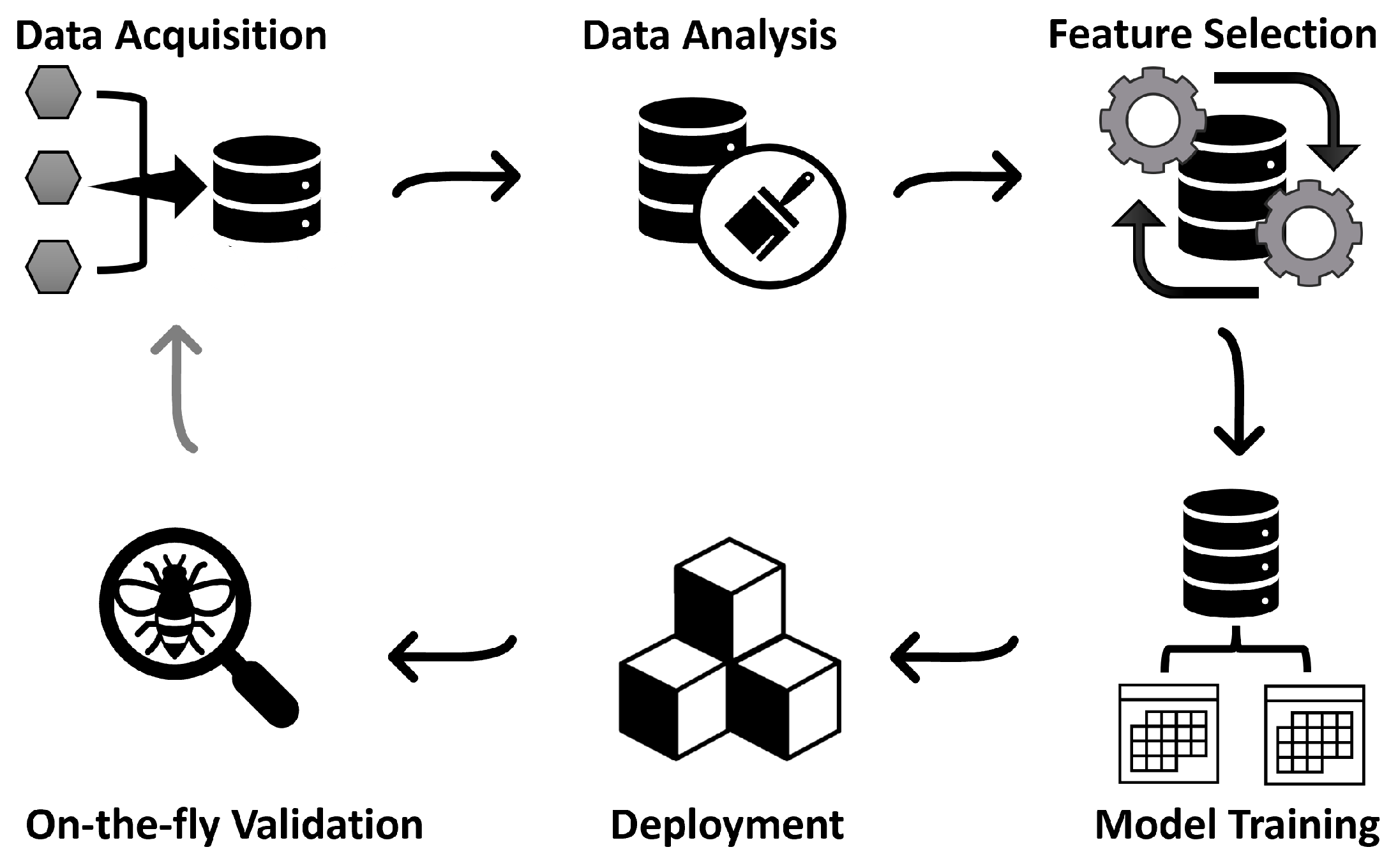
2.3. PowerModel-AI Architecture and Pipeline

The neural network models in this study were implemented in Python (v.3.10.14) using the PyTorch (v.2.2.2) library [18]. All training and test datasets, generated with PowerModels.jl, and the machine learning pipeline, were processed on a Dell Latitude 5430 PC equipped with a 12th Gen Intel^® Core^TM i7-1265U processor (1.8 GHz), 32 GB DDR4 RAM, and 1 TB SSD storage.

Figure 1 illustrates the process from data acquisition to the deployment and on-the-fly criteria assessment of PowerModel-AI. The gray arrow completing the loop from the On-the-fly Validation step back to Data Acquisition indicates that the loop terminates when the on-the-fly criteria are met, meaning the prediction is valid. If the criteria are not met, a new dataset is automatically generated, and the model is updated accordingly.

The step-wise implementation of PowerModel-AI algorithm is showcased as a flowchart in Figure 2, where all symbols follow their conventional meanings [19]. The long rectangular bars denote simultaneous processes. The approach for inferring voltage magnitudes and angles in the AC power flow problem involves constructing four different models to predict the generation active and reactive powers based on load changes (2 models). These predicted values are then used as inputs for two additional models to infer the voltage magnitudes and angles (see model design in Figure 2).

The PowerModel-AI pipeline is divided into three stages: the base, deployment, and on-the-fly stages. In the base stage, the initial model is trained and tested, forming what is referred to as the Base Model. This model is then used to predict voltage responses to new, unseen changes in power demand in the deployment stage.

The on-the-fly stage is triggered when specific criteria are unmet (discussed further in Section 2.5). It operates similarly to the base stage but automatically generates a new dataset using PowerModels.jl in regions where prediction performance is suboptimal. The model built during this stage is called the Updated Model. Unless the user intervenes, the updated model replaces the base model for future runs. Details of each stage are provided below:

• A. Base Stage

• Generate the initial training data using PowerModels.jl (refer to Section 2.2).
• Build the generation active power model. The input features are the new active and reactive power demand in the nodes with load, as well as the preset generation active and reactive power (before any changes in power demand). The target is the new generation active power.
• Repeat Step 2 for the generation reactive power model. The input features remain the same, but the new generation reactive power is set as the target.
• Build the bus voltage magnitude model using the new power demands (active and reactive) and their corresponding generation reactive power as the input feature. The new bus voltage magnitudes are set as the target.
• Repeat Step 4 for bus voltage angles. For the input feature, the generation reactive power replaces its active counterpart. Also, the new bus voltage angles are the target.
• Save all four models for deployment.

• B. Deployment Stage

7.

Import the base models.

8.

User inputs new power demands (active and reactive) for the selected nodes.

9.

Use the generation power models to predict the generation active and reactive power, based on new power demand.

10.

Use the predicted generation power and the new power demand to predict the bus voltage magnitudes and angles.

• C. On-the-Fly Stage

11.

Automate on-the-fly criteria validation using the predicted data from the deployment stage.

12.

If criteria are met, validate results and models. Otherwise,

13.

If criteria fail, compute new power flow data in the failure region using PowerModels.jl, then retrain the base model parameters to obtain the updated model.

14.

If desired, replace the base model with the updated model.

A critical point in the ML architecture is that the generation power models are expected to remain unchanged when there are no variations in power output resulting from fluctuations in power demand. In such cases, the model’s output should ideally replicate the given input. However, the utility of the generation power model becomes particularly evident when changes in power supply occur due to shifts in power demand, either at the slack bus or at nodes equipped with generators.

2.4. PowerModel-AI Hyperparameters

The PyTorch hyperparameters used for model training are detailed in

Table 2. Neural-network hyperparameters implemented in Pytorch.

Hyperparameter	Description	Value
Number of Layers	Total number of hidden layers in the network	2
Batch Size	Number of samples per gradient update	32
Number of Epochs	Total number of passes through the training dataset	300
Learning Rate	Step size for updating weights during training	0.001
Number of Neurons	Number of neurons per hidden layer	Varies a
Loss Function	Evaluates accuracy of the model’s predictions	MSEloss b
Activation Function	Function applied to the output of each neuron	Leaky ReLU
Weight Initialization	Strategy for setting initial weights	Xavier Initializer
Optimization Algorithm	Method for updating weights based on gradients	Adam Optimizer

^a ζ denotes the input feature size. The number of neurons (rounded to the nearest integer) in the first and second layers are ${\displaystyle \frac{\zeta }{3}}$ and ${\displaystyle \frac{\zeta }{6}}$, respectively. The input feature sizes for the generation models (${\zeta }_g$) and voltage models (${\zeta }_v$), are listed in Table 1. ^b The MSEloss criterion in the mean square error loss function in Pytorch.

. The input features were set up by converting the power demand and generation data into PyTorch tensor objects, which were then concatenated. For the power demand, only the active and reactive components for nodes with load were included, while buses without load components were excluded. As a result, the power demand tensor contains only non-zero elements.

For generation power, a one-hot encoding approach was used to represent all nodes in the system. Nodes without generation were assigned zero values in the tensor. Nodes with only reactive generation (i.e., synchronous condensers) had a zero value for active power, while generator nodes (with both active and reactive power) had non-zero elements. This structure ensures the model can distinguish between nodes with no generation, reactive-only generation, and both active and reactive generation power.

While the design for the input features remain consistent for all the ML models, the size of the input feature vector (taken as $\zeta$) varies with the specific synthetic grid. The input feature sizes for the generation (${\zeta }_g$) and voltage (${\zeta }_v$) models are provided in Table 1. For the 500-bus case, which includes 200 nodes with load and 60 nodes with either generators or synchronous condensers, its input feature size is 1400 for the generator models and 900 for the voltage models. In comparison, the sizes are 616 and 416 for the 200-bus, 128 and 91 for the 37-bus, 102 and 72 for the 30-bus, and 50 and 36 for the 14-bus case. All models have two hidden layers, with the first layer having ${\displaystyle \frac{\zeta }{3}}$ neurons and the second layer having ${\displaystyle \frac{\zeta }{6}}$ neurons (both rounded to the nearest integer).

Based on this, the input features used in model training are inherently sparse, with many zero-valued elements. Figure 3a,b illustrate this feature sparsity by showing the layer weights for the generation power and voltage models in the 37-bus grid, respectively.

The Leaky ReLU (Rectified Linear Unit) activation function utilized for training, is given as [20]:

$$g\left(x\right)=\left\{\begin{array}{cc}x\hfill & \mathrm{if}x\ge 0\hfill \\ \alpha x\hfill & \mathrm{if}x<0\hfill \end{array}\right.$$

(9)

where, $\alpha$ (= 0.01) is a small positive constant that defines the slope for negative inputs. This non-zero gradient helps prevent the dying ReLU problem associated with the ReLU activation function, thereby supporting continued learning during backpropagation [20,21]. The loss function, weight initialization, and optimization algorithm were configured using the default settings in Pytorch (see Table 2). The training data was divided into training, validation, and test sets in a 70:15:15 ratio. Additionally, external testsets were generated using the procedure outlined in Section 2.2. These datasets were used to evaluate model performance and form the basis of the results presented in this study.

2.5. The On-the-Fly Learning Implementation

In the current version of PowerModel-AI, three criteria are considered for on-the-fly prediction. Although these criteria may not be universally applicable to all power grid scenarios, they were tested and applied to the grids discussed in this study, offering valuable insights for automating power flow solution predictions. However, the interested reader is encouraged to adapt these criteria to address specific power flow problems. The criteria used are discussed in detail in this section.

2.5.1. Training Domain

The first criterion is based on domain knowledge of the training data. If the changes in power demand fall outside the range of the training domain, there is a reasonably high probability that the predicted voltages will be inaccurate. The load multiplier range, between ${\Delta }_{\min }$ and ${\Delta }_{\max }$, considered for each power grid case in this study is detailed in Table 1. However, since load changes affect individual nodes differently and may not uniformly influence power across all nodes or specific groups of nodes (as discussed in Section 3.1.1), relying solely on this domain-based criterion for on-the-fly predictions is not ideal. Nevertheless, it serves as a useful indicator for potential issues with the model’s prediction performance.

2.5.2. Power Conservation

The second criterion is grounded in the physical principle of energy or power conservation. Specifically, the total power in the grid must equal zero, such that:

$$\sum _{i=1}^D{S}_{i_d}+\sum _{j=1}^G{S}_{j_g}+\sum _{k=1}^K{S}_k^{loss}=0$$

(10)

$S_{i_d}$ and $S_{j_g}$ are defined in Equations (2) and (3), respectively, and $S_k^{loss}$ is the power loss in the kth branch (line or transformer). Following the discussion in Section 2.1, we rewrite Equation (5b) to align with Equation (10), resulting in the power conservation equation:

$$P_{i_g}-j{Q}_{i_g}-P_{i_d}+j{Q}_{i_d}-Y_{i,i}{\left|V_i\right|}^2-V_i^{*}\sum _{j=1,j\ne i}^N{Y}_{i,j}{V}_j\approx 0$$

(11)

It is important to note that the equality in Equation (11) is an approximation due to the inherent errors in any machine learning prediction of the ACPF solutions. Therefore, the power conservation criterion should be assessed relative to the training and test errors obtained during model development. Additionally, other contributing factors, such as the presence of switched shunts that may contribute to reactive power in the system [22], should be considered for specific cases.

2.5.3. Generation Power Saturation

The third criterion is based on the saturation limits of generation power, including that of the swing node. This criterion involves four variables: the maximum and minimum total generations for (1) active power: ${\sigma }_P^{+}$ and ${\sigma }_P^{-}$, and (2) reactive power: ${\sigma }_Q^{+}$ and ${\sigma }_Q^{-}$. The on-the-fly algorithm will be activated only when the following conditions are not met:

$${\sigma }_P^{-}<\sum _{i=1}^G{P}_{i_g}<{\sigma }_P^{+}$$

(12)

and

$${\sigma }_Q^{-}<\sum _{i=1}^G{Q}_{i_g}<{\sigma }_Q^{+}$$

(13)

The values of ${\sigma }_P^{-}$, ${\sigma }_P^{+}$, ${\sigma }_Q^{-}$, and ${\sigma }_Q^{+}$ for the training dataset used in this study are listed in Table 1. Here, $P_{i_g}$ and $Q_{i_g}$ represent the predicted generation active and reactive power outputs from the respective generation models.

3. Result & Discussion

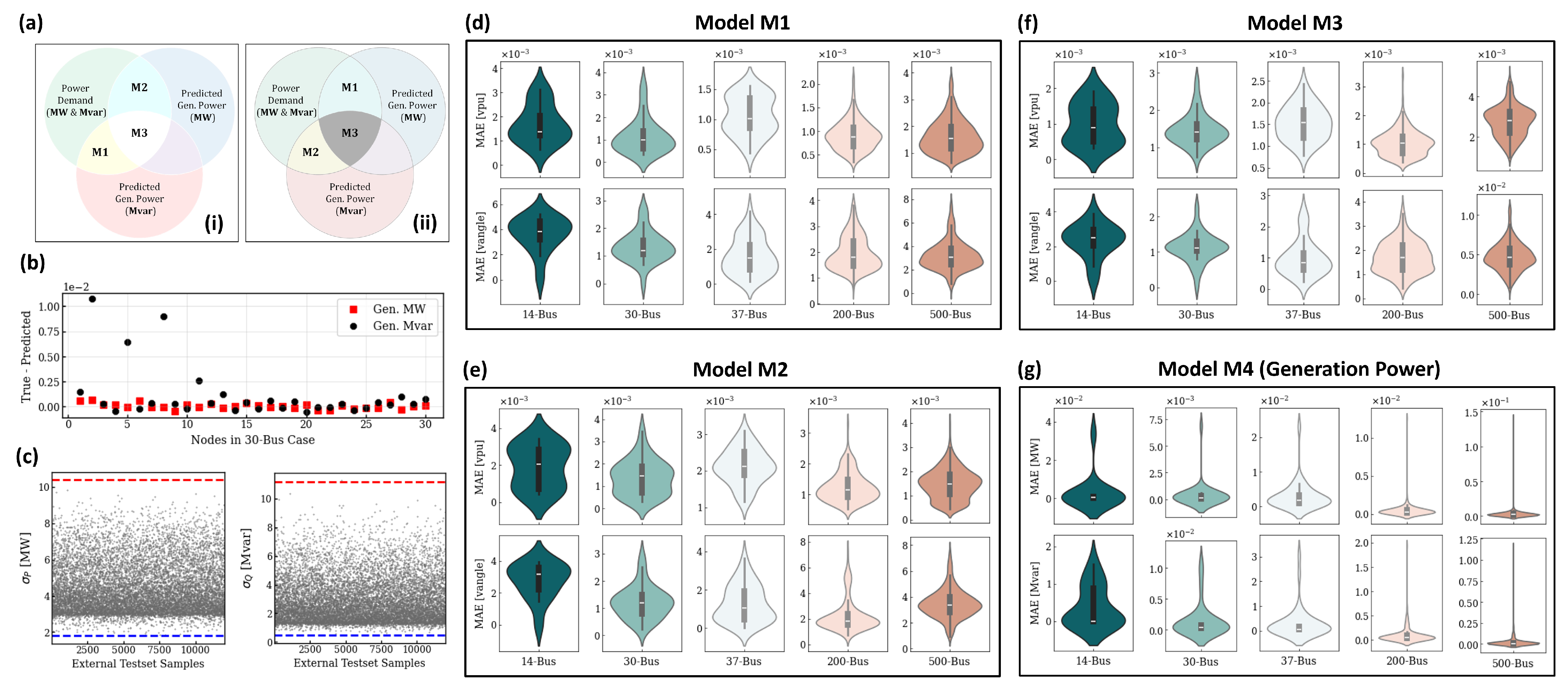
3.1. Model Selection and Assessment

Before selecting the design for PowerModel-AI, we conducted thorough analyses using domain-specific knowledge of synthetic grids and data manipulation techniques to extract meaningful features from the training dataset. This foundational work is crucial for enhancing the model’s predictive capabilities. Details of these analyses and their influence on the model selection process are discussed in this section.

In general, we found that by identifying key input features (such as generation power) and applying one-hot encoding, we achieved satisfactory prediction accuracy with a simple architecture of two hidden layers. This approach suggests that effective feature and model selection can minimize the need for regularization and dropout techniques, which were not incorporated into our design. Furthermore, the training process consistently proved to be effective in 200 to 300 epochs. The supplementary PDF file accompanying this work displays Figures S1–S5, which illustrate the training (red) and validation (blue) loss convergence curves for the PowerModel-AI (M1 model) across the 14-Bus, 30-Bus, 37-Bus, 200-Bus, and 500-Bus synthetic grids. In each case, the model achieves rapid convergence—around the 10th epoch—with the validation loss beginning at a significantly lower value than the training loss.

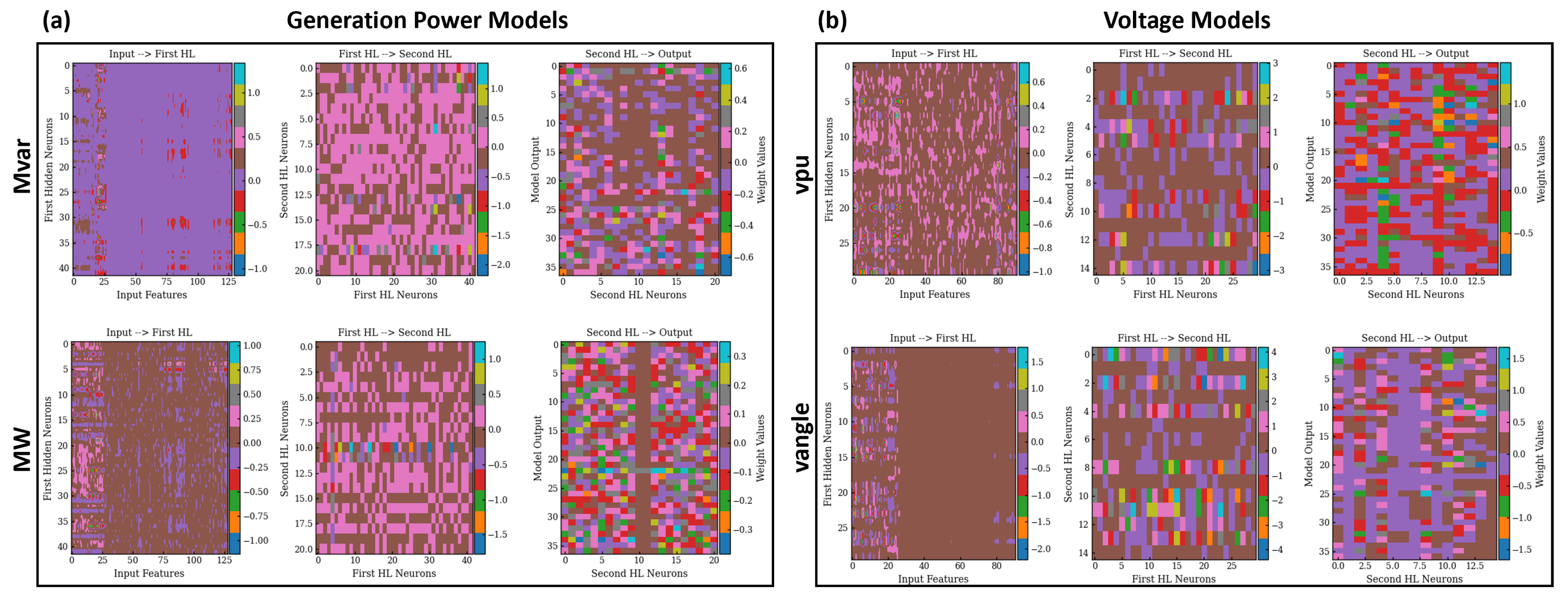
3.1.1. Node Dependencies

The first analysis was to identify correlations between changes in power demand and bus voltages. To investigate this, the sensitivity of bus voltages to changes in power demand was measured as the average deviation of each node’s voltage from its preset value (i.e., before any change in power demand). The data set for the sensitivity analysis was generated as described in Section 2.2, with the key difference being that m (= 2505) random changes to power demand are applied to one single node at a time and repeated for other nodes. Consequently, for each node under consideration, the size of n is always 1. The size of the dataset, $\tau$, is m × the number of nodes with load.

The top panel in Figure 4a–c shows the sensitivity of node voltage magnitudes to load changes in the 14-bus, 30-bus, and 37-bus synthetic grids, respectively. The middle panel illustrates the sensitivity of voltage angles, while the bottom panel provides simplified representations of node connections in the synthetic grids. The color bar indicates the normalized voltage deviation, $V_{n,k}^{\prime }$, for all nodes (k) due to power demands on a specific node (n), calculated as:

$$\begin{array}{cc}\hfill V_{n,k}^{\prime }& ={\displaystyle \frac{{\tilde{V}}_{n,k}}{max\left({\tilde{V}}_{n,k}\forall k\in K\right)}}\hfill \end{array}$$

(14a)

$$\begin{array}{cc}\hfill {\tilde{V}}_{n,k}& ={\displaystyle \frac{1}{V_k^0}}\left|{\displaystyle \frac{1}{M}}\sum _{m=1}^M{V}_{n,k}^m-V_k^0\right|\hfill \end{array}$$

(14b)

Here, M represents the total number of load multipliers within the range from ${\Delta }_{\min }$ to ${\Delta }_{\max }$. $V_k^0$ denotes the initial voltage of the $k\mathrm{th}$ node, while $V_k^m$ represents the voltage at the $k\mathrm{th}$ node after applying the $m\mathrm{th}$ load multiplier to the preset power demand at the $n\mathrm{th}$ node.

From Equations (14a) and (14b), when $V_{n,k}^{\prime }\to 1$ in Figure 4, this indicates a high sensitivity of the $k\mathrm{th}$ node’s voltage (on the x-axis) to changes in power demand at the $n\mathrm{th}$ node (on the y-axis).

The top panel of Figure 4 indicates that the voltage magnitudes of nodes with generators generally remain stable regardless of the changes in power demand, as generators adjust by supplying the additional power. This trend is consistent across all bus cases. However, this was not the case for the voltage angles, where significant variations among the synthetic grids was observed. For example, the swing nodes in the 14-bus (Node 1) and 37-bus (Node 29) systems tend to maintain their original voltage angles at 0° and −2.11°, respectively.

3.1.2. Load Flow Decoupling in Power Systems

A fundamental assumption in power flow equations is that changes in active power are primarily influenced by changes in voltage angles, while changes in reactive power are mainly affected by variations in voltage magnitude. This principle is critical to the Fast Decoupled Load Flow (FDLF) method [23] for solving power flow problems and our models also exhibited this characteristic.

To demonstrate this, we present the voltage prediction performance of three candidate models considered in the standard ML model selection process. Figure 5 and Figure 6 show the prediction accuracy for voltage magnitude and angle, respectively. The plots compare the true or target voltages (x-axis) with predicted or output voltages (y-axis). Data points aligned along the diagonal gray line indicate high prediction accuracy. The color bar represents a non-parametric Gaussian kernel density estimation, normalized to map the density of the true and the predicted values. The red regions (indicating values closer to 1) highlight areas with higher data point concentration, while blue regions (indicating values closer to 0) represent areas with lower concentration. For satisfactory prediction performance, the red regions should closely align with the diagonal gray line.

Figure 4. The Normalized sensitivity of the voltage magnitude (top panel) and angles (center panel) to load changes in the (a) 14-bus, (b) 30-bus cases, and (c) 37-bus cases. The color bar represents the average deviation of the new voltage values from those of the original configuration (before any changes in power demand). A value of 1(0) indicated the most(least) sensitive bus nodes. The bottom panel depicts schematic representations of the grids. Nodes that do not have generators are colored in brown, those having both active and reactive generation power (i.e., generators) are colored green, while nodes with only reactive generation power (i.e., synchronous condenser) are colored yellow. The nodes labeled “1” in the 14-bus and 30-bus systems and “23” in the 37-bus system are the slack (or swing) node.

Figure 4. The Normalized sensitivity of the voltage magnitude (top panel) and angles (center panel) to load changes in the (a) 14-bus, (b) 30-bus cases, and (c) 37-bus cases. The color bar represents the average deviation of the new voltage values from those of the original configuration (before any changes in power demand). A value of 1(0) indicated the most(least) sensitive bus nodes. The bottom panel depicts schematic representations of the grids. Nodes that do not have generators are colored in brown, those having both active and reactive generation power (i.e., generators) are colored green, while nodes with only reactive generation power (i.e., synchronous condenser) are colored yellow. The nodes labeled “1” in the 14-bus and 30-bus systems and “23” in the 37-bus system are the slack (or swing) node.

These predictions were tested on an external dataset of 12,000 data points. For a fair comparison, we focus on the worst-case predictions across the five Texas A&M synthetic grids. The specific bus node is indicated in each plot legend. Similar plots for other nodes across all grids are provided as Supplementary Material, available as PNG files and Jupyter notebooks [17].

Figure 5. Comparison of true (from the external testset) and predicted voltage magnitude (vpu) for control models (C1, C2, C3) and candidate models (M1, M2, and M2), respectively. The bus nodes displayed were selected to show the worst-case predictions and hence the reason for the model selection decision. Similar plots for all buses (and models) are available as Supplementary Datasets [17].

Figure 5. Comparison of true (from the external testset) and predicted voltage magnitude (vpu) for control models (C1, C2, C3) and candidate models (M1, M2, and M2), respectively. The bus nodes displayed were selected to show the worst-case predictions and hence the reason for the model selection decision. Similar plots for all buses (and models) are available as Supplementary Datasets [17].

Figure 6. Corresponding plot for the comparison of the true and predicted voltage angle, with the same intent as discussed for the voltage angles in Figure 5. The brown arrow highlights a deviation in the 76th node for M2. Similar plots for the remaining nodes are also available as Supplementary Datasets [17].

Figure 6. Corresponding plot for the comparison of the true and predicted voltage angle, with the same intent as discussed for the voltage angles in Figure 5. The brown arrow highlights a deviation in the 76th node for M2. Similar plots for the remaining nodes are also available as Supplementary Datasets [17].

In Figure 5 and Figure 6, the left panel plots labeled C1, C2, and C3 represent the control models, while the right panel plots labeled M1, M2, and M3 are the candidate models for PowerModel-AI algorithm. The key difference between these two sets of models lies in their approach to incorporating the generation power data. The control models use generation power directly from the training dataset as input features, bypassing the generation ML model (henceforth referred to as M4) entirely. In contrast, the candidate models first predict generation power using M4 and then use these predicted values as part of their input features for the voltage prediction. This approach requires only changes in power demand as the original input feature (see the algorithm flowchart in Figure 2). As a result, the control models undergo a single training and prediction stage, whereas the candidate models involve a two-stage process. Given this streamlined approach, the control models are expected to provide more accurate predictions, hence their designation as “control”.

The numbers “1”, “2”, and “3” in the model labels indicate that models with the same number share the same type of input features. The Venn diagrams in Figure 7a illustrate the input features used for predicting (i) the voltage magnitude and (ii) the voltage angle in the candidate models. Similar diagrams can be created for the control models by replacing “M” with “C” and substituting the predicted generation power with the true generation power. All models include the updated active and reactive power demands as their input features. In addition to this:

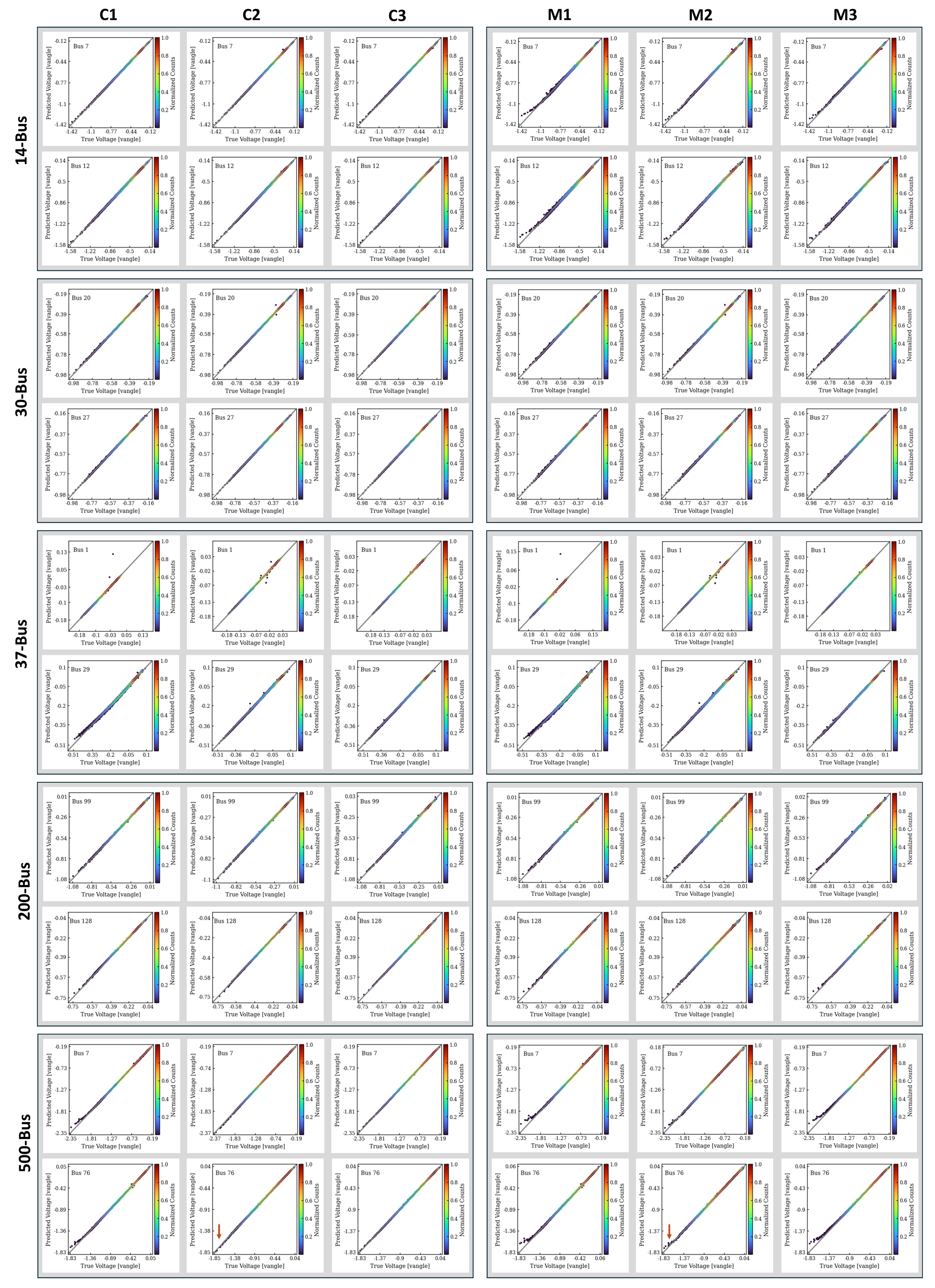
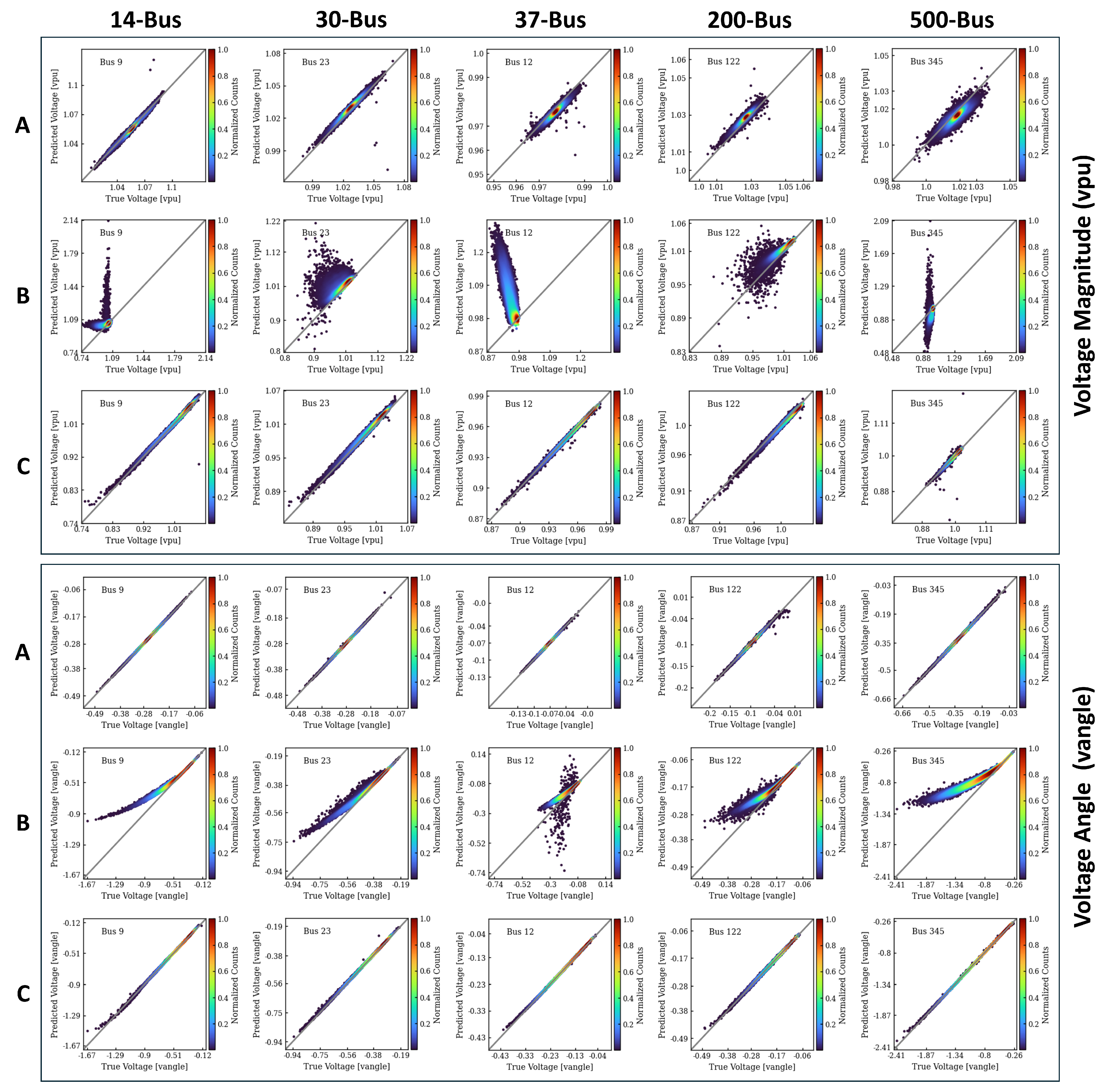
• M1 (C1) includes the predicted (true) generation reactive power for the voltage magnitude prediction and the active generation power for voltage angle prediction.
• M2 (C2) uses the predicted (true) generation reactive power to infer the voltage angles and the active generation power for voltage magnitude.
• M3 (C3) incorporates both the predicted (true) reactive and active generation power to infer the voltage magnitude and angles.

Overall, the voltage plots for the candidate models closely mirror those of their corresponding control models, suggesting that the generator model, M4, accurately predicts the true generation power. This alignment is particularly notable since the use of predicted versus actual generation power is the only difference between the two kinds of models. We illustrate this in Figure 7b, where the mean differences between true and predicted generation active and reactive powers are plotted for all nodes in the 30-bus grid. Additionally, Figure 7c shows that the total power of the external test-set are within the generation power limits for the 30-bus, specified in Table 1 and discussed in Section 2.5.3. The red and blue dashed lines indicated the upper and lower generation power limit, respectively.

As noted earlier, Figure 5 and Figure 6 depict the worst-case prediction scenarios. For the M1 model’s voltage magnitude predictions, while some data points deviate from the diagonal (especially in the 14-bus case), the red density regions remain centered along the diagonal, indicating overall satisfactory prediction performance across all grids.

In contrast, the M2 and M3 model predictions for the 37-, 200-, and 500-bus synthetic grids show that the red density regions are not consistently aligned with the diagonal, although the data points are not significantly scattered. This misalignment points to potential underfitting or overfitting, likely due to an unfavorable bias-variance tradeoff (high bias, low variance) [24]. Notably, this issue does not arise in the M1 model predictions, where the red density regions consistently align with the diagonal, signifying more robust performance.

The voltage angle prediction plots in Figure 6 generally demonstrate better fitting quality across all candidate models. However, some discrepancies between the candidate models and their respective control models are noticeable, particularly in the lower voltage regions of the 14- and 500-bus cases. For instance, the brown arrow highlights a deviation in the 76th node plot for the M2 model. While this difference may seem minor due to its occurrence in areas with the lowest data density (blue region), a comparison across models reveals that M1 maintains better consistency with its control model. Models M2 and M3 exhibit these discrepancies, despite their control models aligning almost perfectly with the diagonal axis, raising concerns about the generalization of their predictions.

These observations further highlight the importance of including generation power as a feature and underscore the critical choice of generation type for accurate voltage magnitude and angle predictions. They also indicate that the M1 model design is optimal for predicting both voltage magnitude and angle, effectively capturing the relationships between active (reactive) power and voltage angle (magnitude).

To further substantiate M1 as the optimal model, we present the mean absolute error (MAE) for all models, depicted as violin plots in Figure 7d–f, and g for M1, M2, M3, and M4, respectively. The MAE for all candidate models is in the ${10}^{-3}$ range, except for the voltage angle MAE in M3, which is in the ${10}^{-2}$ range. Notably, M1 consistently demonstrates a lower MAE compared to M2 and M3, affirming its superior performance. Additionally, the mean squared error (MSE) test losses for M1, detailed in Table 1, further confirm its satisfactory performance during training.

Consequently, previous and subsequent references to PowerModel-AI relate to the design of the M1 model. To further validate M1, we show in

Table 3. Mean absolute error (MAE) and mean square error (MSE) for PowerModel-AI (M1) compared to PowerModel.jl iterative solver over 12,000 independent loading events.

	MAE $\left[\times {10}^{-3}\right]$				MSE $\left[\times {10}^{-6}\right]$
Grid	$\mathit{vpu}$	$\angle \mathit{v}$	MW	MVAR	$\mathit{vpu}$	$\angle \mathit{v}$	lMW	MVAR
14-Bus	1.71	3.66	3.00	3.82	2.92	13.4	8.98	14.6
30-Bus	1.16	1.33	0.43	1.46	1.35	1.76	0.19	2.13
37-Bus	1.07	1.61	2.94	3.08	1.14	2.60	8.62	9.47
200-Bus	0.92	1.96	0.47	1.02	0.84	3.85	0.23	1.03
500-Bus	1.63	3.18	3.00	2.45	2.67	10.1	9.00	6.01

, the MAE and MSE of M1 compared to the output of PowerModel.jl for 12,000 independent loading events. The plot of the training losses for all the models discussed in this work is provided as Supplementary Data in the Jupyter notebooks [17]. All models show good convergence in the training and validation sets.

3.2. On-the-Fly Model Update

A key innovation of PowerModel-AI is its on-the-fly feature, which minimizes the need to generate training data for every possible scenario as the learning protocol is automated based on prediction performance. The query strategy used in PowerModel-AI is based on the three criteria discussed in Section 2.5: (1) the training domain, (2) power conservation, and (3) generation power saturation. For this study, and based on the analysis presented herein, we opted to assign a scoring metric to determine when to initiate on-the-fly learning. The scoring metric, on a scale of 5, is allocated as follows:

• Training Domain Criterion → 1 points
• Power Conservation Criterion → 1 points
• Generation Power Saturation Criterion → 3 points

In the PowerModel-AI implementation, a score is awarded if the predicted result satisfies a criterion, otherwise, no score is given. A minimum score of 4 points is required during any prediction to avoid initiating a model update. Therefore, on-the-fly learning is triggered if a set of load changes fails to meet the 4-point threshold.

The Training Domain Criterion is assigned a score of 1 because not all buses with loads equally contribute to power redistribution or significantly influence voltage outputs. Moreover, deviations from the current training domain can result in infeasible solutions within PowerModels.jl, which fall outside the scope of AC power flow problems considered here–becoming optimal power flow [25,26,27] or contingency analysis [28,29,30] problems.

Similarly, the Power Conservation Criterion also receives a score of 1, as its outcome is influenced by inherent training errors in both M1 and M4, although it generally holds true in most cases. The Generation Power Saturation Criterion, however, is given the highest score of 3, as our findings show that generation power is critical for model selection. Thus, adhering to the default power limits in the training set is essential for ensuring valid results.

To demonstrate the advantages of PowerModel-AI’s on-the-fly learning capability, we compare the voltage magnitude and angle prediction performance of two M1 models, shown in the upper and lower panels of Figure 8, respectively. The first model, which is the base model, was trained on a dataset generated using a load multiplier upper limit of 2.0, denoted as ${\Delta }_{\max }^{*}$. The details of this dataset are provided in

Table 4. Details of the new training dataset used to demonstrate PowerModel-AI’s on-the-fly learning feature. All parameters follow the definitions in Table 1, with the values for $\tau$ and ${\Delta }_{\min }^{*}$ remaining the same. Asterisks indicate that this training dataset differs from the one in Table 1.

Parameters	14-Bus	30-Bus	37-Bus	200-Bus	500-Bus
${\Delta }_{\max }^{*}$	2.0	2.0	2.0	2.0	2.0
${\sigma }_P^{-*}$	0.830	1.261	7.007	16.381	42.273
${\sigma }_P^{+*}$	4.897	5.080	17.144	28.805	60.734
${\sigma }_Q^{-*}$	−0.172	0.091	−0.197	2.338	−2.939
${\sigma }_Q^{+*}$	2.642	3.347	0.830	10.786	12.379

, where the asterisks indicate that the parameters differ from those used in the dataset described in Table 1.

The second model is the base model retrained on the external testset used in Figure 5 and Figure 6, now serving as a new training dataset. This second model, referred to as the updated model (as defined in Section 2.3), was trained using the parameters outlined in Table 1, specifically with ${\Delta }_{\max }$. Notably, both datasets share the same values for $\tau$ and ${\Delta }_{\min }$.

In Figure 8, the “A” rows show the base model’s prediction performance on an external test set generated using ${\Delta }_{\max }^{*}$. Rows “B” and “C” depict the base and updated models’ performance on a new, unseen external test set generated with ${\Delta }_{\max }$. It is evident that while the base model performs well in the ${\Delta }_{\max }^{*}$ domain (row A), it fails to generalize to the ${\Delta }_{\max }$ domain (row B). However, after on-the-fly implementation, the updated model shows improved prediction performance in the ${\Delta }_{\max }$ domain (row C).

We note that the nodes plotted in Figure 8 were selected based on the base model’s best-case predictions for the ${\Delta }_{\max }$ dataset in Row B. Similar plots for other nodes are available as Supplementary Material [17]. Importantly, Table 4 indicates that the on-the-fly criteria were not met for the predictions in Row B. Therefore, in PowerModel-AI’s operational scenario, the on-the-fly model update algorithm would have been triggered.

3.3. The PowerModel-AI Software Application

PowerModel-AI is available as open-source software hosted on Streamlit [16]. The algorithm is also accessible on LANL’s Advanced Network Science Initiative (ANSI) GitHub page (https://github.com/lanl-ansi/PowerModelsAI/tree/main (accessed on 28 March 2025)). In the current version, the training datasets for the base and updated models are automatically generated using the PowerModels.jl package—an open-source power flow solver/optimizer developed at LANL. Users have the option to integrate their preferred iterative solver.

4. Conclusions and Prospects

In power systems, determining power injection from known network voltages is relatively straightforward. However, the inverse problem—calculating voltages from given power injections—presents a significant challenge due to the nonlinearity of power flow equations. This study introduces PowerModel-AI, a new machine learning software that leverages historical AC power flow data to accurately predict solutions for power demands in synthetic grids. The neural network models are constructed with two hidden layers, each having a carefully selected number of neurons to balance model complexity with computational efficiency, ensuring that the network effectively learns meaningful patterns from the data without over- or under-fitting. We provide prediction results and analyses for five Texas A&M synthetic power grid cases: the 14-, 30-, 37-, 200-, and 500-bus systems.

PowerModel-AI features a state-of-the-art online learning routine known as on-the-fly learning. This approach offers two main benefits: (1) it minimizes the need to generate training data for every possible scenario, and (2) it enables instantaneous model updates when the model’s predictions diverge from accuracy. The updates are based on three criteria: (a) the range of the training domain, (b) principles of power/energy conservation, and (c) generation power saturation limits. Our results underscore the importance of careful model selection, particularly in input feature selection. The model design effectively captures the relationship between active/reactive power and voltage angle/magnitude, adhering to the load flow decoupling principle.

To support reproducibility and encourage open research, we have made the datasets and models used in this study publicly available. Additionally, we provide access to the PowerModel-AI online application, hosted on Streamlit, along with all representative plots (both presented and not presented in this study) and the algorithms (Python scripts in Jupyter notebooks) used to generate them.

Looking ahead, future developments for PowerModel-AI will focus on expanding its prediction capabilities to include optimal power flow, contingency analysis, and predicting infeasible solutions based on specified power demands. Currently, PowerModel-AI aggregates generation powers at nodes with multiple generator fuel types, but future versions will address this by explicitly specifying generator fuel types, potentially enhancing the model’s predictive accuracy in complex scenarios.

References

1. Chatterjee, S.; Mandal, S. A novel comparison of gauss-seidel and newton- raphson methods for load flow analysis. In Proceedings of the 2017 International Conference on Power and Embedded Drive Control (ICPEDC), Chennai, India, 16–18 March 2017; pp. 1–7. [Google Scholar] [CrossRef]
2. Glover, J.D.; Overbye, T.J.; Sarma, M.S. Power System Analysis & Design, 6th ed.; Cengage Learning: Boston, MA, USA, 2017; Chapter 6. [Google Scholar]
3. Fikri, M.; Haidi, T.; Cheddadi, B.; Sabri, O.; Majdoub, M.; Aziz, B. Power Flow Calculations by Deterministic Methods and Artificial Intelligence Method. Int. J. Adv. Eng. Res. Sci. 2018, 5, 148–152. [Google Scholar] [CrossRef]
4. Huang, B.; Wang, J. Applications of Physics-Informed Neural Networks in Power Systems - A Review. IEEE Trans. Power Syst. 2023, 38, 572–588. [Google Scholar] [CrossRef]
5. Bolz, V.; Rueß, J.; Zell, A. Power Flow Approximation Based on Graph Convolutional Networks. In Proceedings of the 2019 18th IEEE International Conference On Machine Learning And Applications (ICMLA), Boca Raton, FL, USA, 16–19 December 2019; pp. 1679–1686. [Google Scholar] [CrossRef]
6. Pham, T.; Li, X. Neural Network-based Power Flow Model. In Proceedings of the 2022 IEEE Green Technologies Conference (GreenTech), Houston, TX, USA, 30 March–1 April 2022; pp. 105–109. [Google Scholar] [CrossRef]
7. Fikri, M.; Sabri, O.; Cheddadi, B. Calculating voltage magnitudes and voltage phase angles of real electrical networks using artificial intelligence techniques. Int. J. Electr. Comput. Eng. (2088-8708) 2020, 10, 5749–5757. [Google Scholar] [CrossRef]
8. Lopez-Garcia, T.B.; Domínguez-Navarro, J.A. Graph Neural Network Power Flow Solver for Dynamical Electrical Networks. In Proceedings of the 2022 IEEE 21st Mediterranean Electrotechnical Conference (MELECON), Palermo, Italy, 14–16 June 2022; pp. 825–830. [Google Scholar] [CrossRef]
9. Liao, W.; Bak-Jensen, B.; Pillai, J.R.; Wang, Y.; Wang, Y. A Review of Graph Neural Networks and Their Applications in Power Systems. J. Mod. Power Syst. Clean Energy 2022, 10, 345–360. [Google Scholar] [CrossRef]
10. Birchfield, A.B.; Xu, T.; Gegner, K.M.; Shetye, K.S.; Overbye, T.J. Grid Structural Characteristics as Validation Criteria for Synthetic Networks. IEEE Trans. Power Syst. 2017, 32, 3258–3265. [Google Scholar] [CrossRef]
11. Coffrin, C.; Bent, R.; Sundar, K.; Ng, Y.; Lubin, M. PowerModels.jl: An Open-Source Framework for Exploring Power Flow Formulations. In Proceedings of the 2018 Power Systems Computation Conference (PSCC), Dublin, Ireland, 11–15 June 2018; pp. 1–8. [Google Scholar] [CrossRef]
12. Doerr, S.; De Fabritiis, G. On-the-Fly Learning and Sampling of Ligand Binding by High-Throughput Molecular Simulations. J. Chem. Theory Comput. 2014, 10, 2064–2069. [Google Scholar] [CrossRef] [PubMed]
13. Jinnouchi, R.; Miwa, K.; Karsai, F.; Kresse, G.; Asahi, R. On-the-Fly Active Learning of Interatomic Potentials for Large-Scale Atomistic Simulations. J. Phys. Chem. Lett. 2020, 11, 6946–6955. [Google Scholar] [CrossRef] [PubMed]
14. Li, Z.; Kermode, J.R.; De Vita, A. Molecular dynamics with on-the-fly machine learning of quantum-mechanical forces. Phys. Rev. Lett. 2015, 114, 096405. [Google Scholar] [CrossRef] [PubMed]
15. Stippell, E.; Alzate-Vargas, L.; Subedi, K.N.; Tutchton, R.M.; Cooper, M.W.; Tretiak, S.; Gibson, T.; Messerly, R.A. Building a DFT+U machine learning interatomic potential for uranium dioxide. Artif. Intell. Chem. 2024, 2, 100042. [Google Scholar] [CrossRef]
16. Ugwumadu, C.; Tabarez, J.; Drabold, D.; Pandey, A. PowerModel-AI Software. Available online: https://powermodel-ai.streamlit.app/ (accessed on 28 March 2025).
17. Ugwumadu, C.; Tabarez, J.; Drabold, D.; Pandey, A. [Data set] PowerModel-AI: A First On-the-fly Machine-Learning Predictor for AC Power Flow Solutions. Zenodo, Version 1; 2024. Available online: https://doi.org/10.5281/zenodo.13843934 (accessed on 28 March 2025).
18. Paszke, A.; Gross, S.; Massa, F.; Lerer, A.; Bradbury, J.; Chanan, G.; Killeen, T.; Lin, Z.; Gimelshein, N.; Antiga, L.; et al. PyTorch: An Imperative Style, High-Performance Deep Learning Library. In Advances in Neural Information Processing Systems; Curran Associates, Inc.: Red Hook, NY, USA, 2019; Volume 32, pp. 8024–8035. [Google Scholar]
19. Schultheiss, L.A.; Heiliger, E.M. Techniques of flow-charting. In Proceedings of the 1963 Clinic on Library Applications of Data Processing; Graduate School of Library Science: University of Illinois, Urbana-Champaign, IL, USA, 1963; pp. 62–78. [Google Scholar]
20. Maas, A.L.; Hannun, A.Y.; Ng, A.Y. Rectifier nonlinearities improve neural network acoustic models. In Proceedings of the 30th International Conference on Machine Learning, Atlanta, GA, USA, 17–19 June 2013; Volume 30, p. 3. [Google Scholar]
21. Bai, Y. RELU-Function and Derived Function Review. SHS Web Conf. 2022, 144, 02006. [Google Scholar] [CrossRef]
22. PowerWorld Corporaton. Switched Shunt Display. Available online: https://www.powerworld.com/WebHelp/Content/MainDocumentation_HTML/Switched_Shunt_Display.htm (accessed on 6 April 2025).
23. Stott, B.; Alsac, O. Fast Decoupled Load Flow. IEEE Trans. Power Appar. Syst. 1974, PAS-93, 859–869. [Google Scholar] [CrossRef]
24. Geman, S.; Bienenstock, E.; Doursat, R. Neural networks and the bias/variance dilemma. Neural Comput. 1992, 4, 1–58. [Google Scholar] [CrossRef]
25. Charles, P.; Mehazzem, F.; Soubdhan, T. A Review on Optimal Power Flow Problems: Conventional and Metaheuristic Solutions. In Proceedings of the 2020 2nd International Conference on Smart Power & Internet Energy Systems (SPIES), Bangkok, Thailand, 15–18 September 2020; pp. 577–582. [Google Scholar] [CrossRef]
26. Yang, K.; Gao, W.; Fan, R. Optimal Power Flow Estimation Using One-Dimensional Convolutional Neural Network. In Proceedings of the 2021 North American Power Symposium (NAPS), College Station, TX, USA, 14–16 November 2021; pp. 1–6. [Google Scholar] [CrossRef]
27. Gan, L.; Low, S.H. Optimal power flow in direct current networks. In Proceedings of the 52nd IEEE Conference on Decision and Control, Firenze, Italy, 10–13 December 2013; pp. 5614–5619. [Google Scholar] [CrossRef]
28. Chen, Q.; McCalley, J. Identifying high risk N-k contingencies for online security assessment. IEEE Trans. Power Syst. 2005, 20, 823–834. [Google Scholar] [CrossRef]
29. Huang, Z.; Chen, Y.; Nieplocha, J. Massive contingency analysis with high performance computing. In Proceedings of the 2009 IEEE Power & Energy Society GeneralMeeting, Calgary, AB, Canada, 26–30 July 2009; pp. 1–8. [Google Scholar] [CrossRef]
30. Tabassum, A.; Chinthavali, S.; Lee, S.; Stenvig, N.; Kay, B.; Kuruganti, T.; Aditya Prakash, B. Efficient Contingency Analysis in Power Systems via Network Trigger Nodes. In Proceedings of the 2021 IEEE International Conference on Big Data (Big Data), Orlando, FL, USA, 15–18 December 2021; pp. 1964–1973. [Google Scholar] [CrossRef]
Figure 1. Overview of the PowerModel-AI pipeline. The gray arrow connecting on-the-fly (post-deployment) validation and data acquisition signifies that this step occurs only when the on-the-fly criteria are unmet.
Energies 18 01968 g001
Figure 2. The flowchart for PowerModel-AI implementation. MW and Mvar are the units for the active and reactive power, respectively. Gen MW, Gen Mvar, Bus vpu, and Bus vangle are colored orange to show that they are the targets in that training phase. All the flowchart shapes adhere to their conventional interpretations.
Energies 18 01968 g002
Figure 3. Representation of the weights in the network layers for (a) generation power and (b) voltage models in the 37-Bus synthetic grid.
Energies 18 01968 g003
Figure 7. (a) Venn diagram depicting the input features for candidate models M1, M2, and M3, used for bus voltage (i) magnitude [vpu] and (ii) angles [vangle] predictions. (b) The generation power (active and reactive) for the original configuration (no change in power demand) and the mean (average) of the predicted values from model M1. (c) The total power values for the external dataset (criteria 3 for on-the-fly). The upper and lower limits obtained from the training set for σ P and σ Q are shown in red and blue, respectively. Violin plot of the prediction mean absolute error (MAE) of models (d) M1, (e) M2, (f) M3, and (g) the power generation model, M4. The mean values are calculated for each node in the external test-set for the different bus cases.
Energies 18 01968 g007
Figure 8. Comparison of true vs. predicted voltage magnitudes (upper panel) and angles (lower panel) to highlights the benefits of PowerModel-AI’s on-the-fly learning capability. In each panel, row A shows the base model’s performance on an external test set from the Δ max * domain, while rows B and C present the performance of the base and updated models on a new external test set from the Δ max domain, as outlined in Table 1. The nodes in the plots are selected based on the base model’s best predictions for the Δ max domain (Row B).
Energies 18 01968 g008