Article

A Short-Term Load Forecasting Method Considering Multiple Factors Based on VAR and CEEMDAN-CNN-BILSTM

1
State Grid Anhui Economic and Technical Research Institute, Hefei 230022, China
2
School of Electrical Engineering and Automation, Hefei University of Technology, Hefei 230009, China
*
Author to whom correspondence should be addressed.
Energies 2025, 18(7), 1855; https://doi.org/10.3390/en18071855
Submission received: 22 February 2025 / Revised: 29 March 2025 / Accepted: 31 March 2025 / Published: 7 April 2025
(This article belongs to the Section F: Electrical Engineering)

Abstract

:
Short-term load is influenced by multiple external factors and shows strong nonlinearity and volatility, which increases the forecasting difficulty. However, most of existing short-term load forecasting methods rely solely on the original load data or take into account a single external factor, which results in significant forecasting errors. To improve the forecasting accuracy, this paper proposes a short-term load forecasting method considering multiple contributing factors based on VAR and CEEMDAN-CNN- BILSTM. Firstly, multiple contributing factors strongly correlated with the short-term load are selected based on the Spearman correlation analysis, the vector autoregressive (VAR) model with multivariate input is derived, and the Levenberg–Marquardt algorithm is introduced to estimate the model parameters. Secondly, the complete ensemble empirical mode decomposition with adaptive noise (CEEMDAN) algorithm and permutation entropy (PE) criterion are combined to decompose and reconstruct the original load data into multiple relatively stationary mode components, which are respectively input into the CNN-BILTSM network for forecasting. Finally, the sine–cosine and Cauchy mutation sparrow search algorithm (SCSSA) is used to optimize the parameters of the combinative model to improve the forecasting accuracy. The actual simulation results utilizing the Australian data validate the forecasting accuracy of the proposed model, achieving reduction in the root mean square error by 31.21% and 18.04% compared to the VAR and CEEMDAN-CNN-BILSTM, respectively.

1. Introduction

Accurate load forecasting is the premise to maintain an active power balance and ensuring the safe operation of a power system, which is helpful to rationally arrange the configurations and maintenance plans of thermal power units and enhance the utilization of new energy sources [1,2,3,4]. In comparison with medium- or long-term electrical energy forecasting with the time scale of a month or year, short-term electrical power forecasting with the time scale of an hour is more sensitive to changing factors, e.g., temperature and electrical price, and shows strong nonlinearity [5,6,7,8]. The gradual implementation of demand-side management policies based on time-of-sale prices and incentives has intensified the nonlinear and random features of the load data, increasing the difficulty of short-term load forecasting [9,10,11].
The existing short-term power forecasting methods may be classified into the mathematical statistics methods and machine learning methods [12]. The former includes multiple linear regression [13], the Kalman filter [14,15], the autoregressive integrated moving average model [16,17], etc., which has a concrete theoretical background. The modeling is easy, and the parameters have good interpretability. They take into account the current load, the contributing factors, and the relationship between the current and past loads [18]. However, their nonlinear fitting ability is weak, and the computational complexity will increase significantly when the model order is high.
The load forecasting based on the machine learning method includes support vector machine [19,20], random forest [21,22], the long short-term memory (LSTM) network [23], and so on. Ref. [24], aiming at the high volatility of a large-scale residential load, built a LSTM network to solve the problem of vanishing and exploding gradients in the recurrent neural network, but it only extracted the forward dependence relationship of the load time series, resulting in low utilization. Ref. [25] built a bidirectional long short-term memory (BILSTM) neural network and employed the grey wolf algorithm to optimize the parameters, improving the forecasting accuracy. However, its global search ability is weak, making it prone to the local optimal solution. Compared to the mathematical statistics method, these models have stronger nonlinear fitting ability and higher forecasting accuracy, but they suffer from poor interpretability, struggle with processing correlations among multiple input variables, and focus primarily on short-term load data [26]. Refs. [27,28] analyzed the impact of contributing factors on short-term loads, highlighting that the changes in electricity price, temperature, and other factors of the load that cannot be ignored.
Some scholars have combined the machine learning method and the data decomposition algorithm and applied them in the field of load forecasting. Ref. [29] adopted empirical mode decomposition (EMD) to decompose the load data into multiple intrinsic mode functions (IMFs) with frequencies ranging from high to low without specifying the basis function and the number of decomposition layers, but there was the problem of mode mixing. Refs. [30,31] decomposed the original load data into multiple mode functions by constructing a variational model, but the number of decomposition times and penalty factors were difficult to select, and the parameters given by experience alone could not meet the actual demand. Ref. [32] decomposed the original load data into multiple relatively stationary IMFs based on complete ensemble empirical mode decomposition with adaptive noise (CEEMDAN), reducing the volatility and non-stationarity of the original load. However, this approach can lead to increased data dimension and reduced operating efficiency. The comparison of different references is given in Table 1.
Based on the above discussion, this study integrates the multivariate time series analysis ability of the mathematical statistics method with the nonlinear fitting advantage of the machine learning method and proposes a short-term load forecasting method considering multiple contributing factors based on VAR and CEEMDAN-CNN-BILSTM. The key contributions of this research are as follows:
(1)
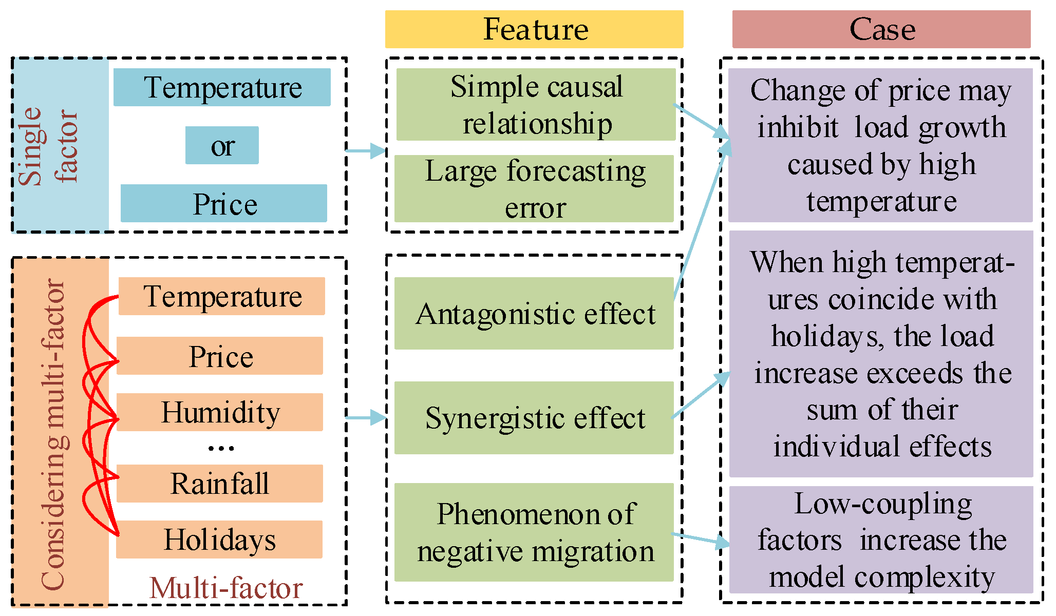
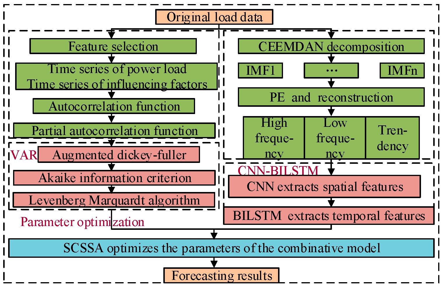
By analyzing the error source of the short-term load forecasting, multiple factors strongly correlated with the short-term load data are selected based on the Spearman correlation coefficient. The vector autoregressive model (VAR) with multivariate input is then derived and improved by using the Levenberg–Marquardt algorithm to estimate the model parameters.
(2)
To reduce the randomness and volatility of the short-term load, CEEMDAN and permutation entropy (PE) are combined to decompose and reconstruct the original load data into multiple relatively stationary mode components, which are respectively input into the CNN-BILTSM model for forecasting.
(3)
The improved VAR with multivariate input is combined with the CEEMDAN-CNN-BILSTM model, and the sine–cosine and Cauchy mutation sparrow search algorithm (SCSSA) is adopted to optimize the parameters of the combinative model to improve the forecasting accuracy.
The structure of this paper is as follows. Section 2 researches the principles of the VAR model with multivariate input. Section 3 describes the CEEMDAN-CNN-BILSTM model. Section 4 proposes a short-term load forecasting method considering multiple contributing factors based on VAR and CEEMDAN-CNN-BILSTM. Section 5 validates this method using actual load data from Australia. The conclusions are given in Section 6.

2. Load Forecast Considering Multi-Factors Using the VAR Model

The short-term load data are sensitive to the changes of several contributing factors, and the relationships among them show strong nonlinearity, as illustrated in Figure 1. For example, the high price may suppress the load growth caused by high temperature. However, most of the existing short-term load forecasting methods rely solely on the original load or consider a single external factor, which results in significant error. The introduction of low-coupling factors may yield the phenomenon of negative migration, increase the model complexity, and reduce the forecasting accuracy. Therefore, it is practical to select the contributing factors strongly correlated to the load as the input variables.
To consider the impact of multiple contributing factors on the load forecasting and reduce the volatility and randomness of the load data, this study proposes a short-term load forecasting method based on VAR and CEEMDAN-CNN-BILSTM to enhance the forecasting accuracy, and its structure is illustrated in Figure 2.

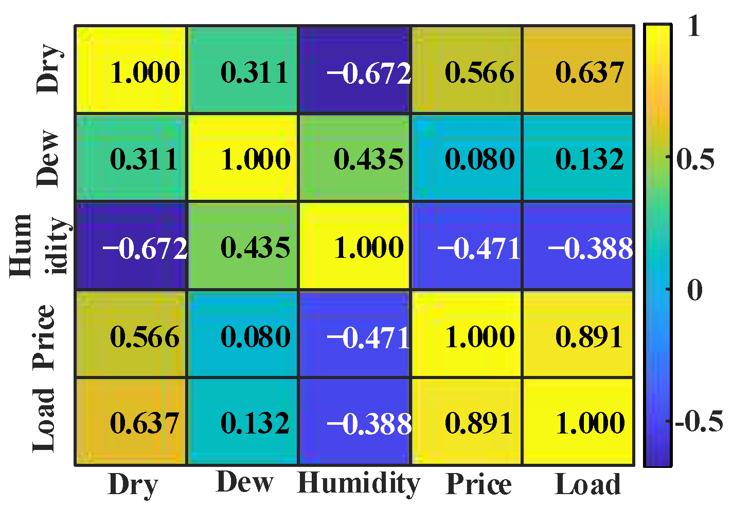
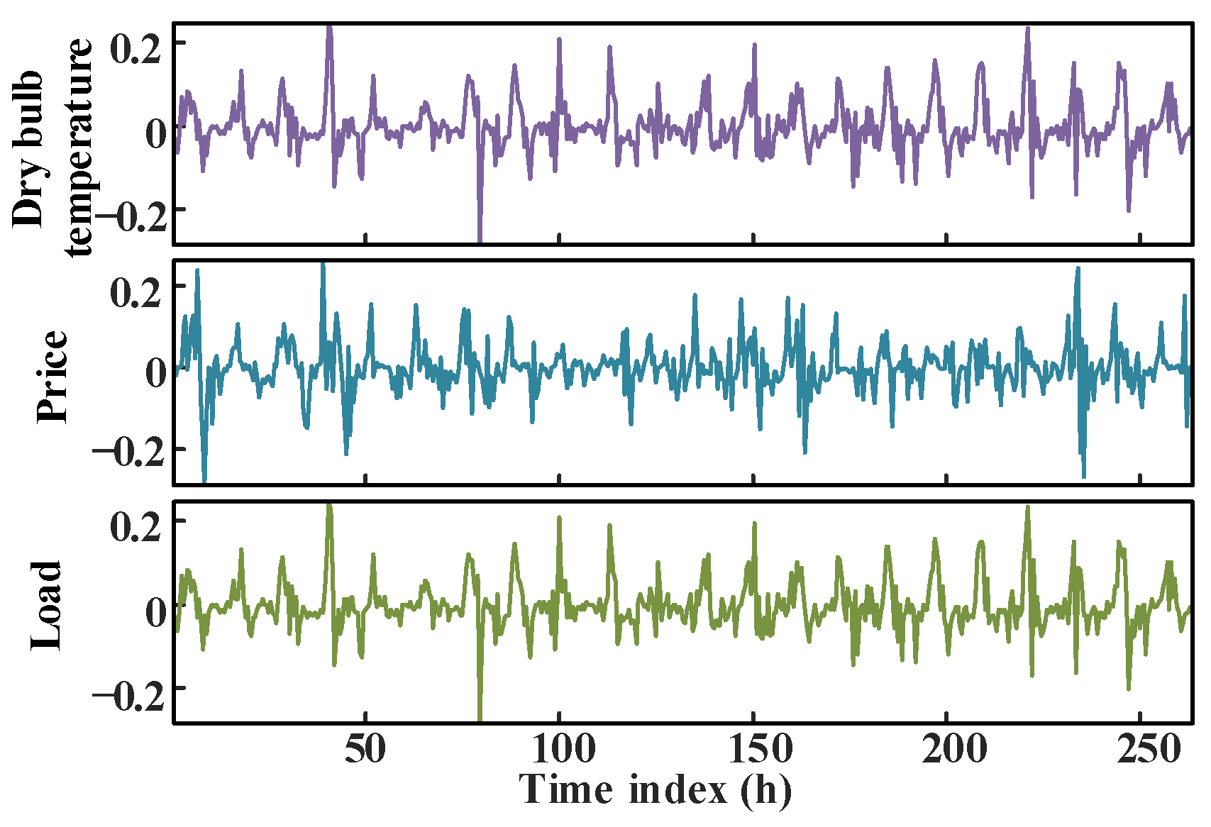
2.1. Feature Selection Based on the Spearman Correlation Coefficient

Considering the nonlinear relationship between the short-term load and contributing factors, the Spearman correlation coefficient is adopted to conduct feature selection on the collected data [18], as shown in Equation (1). To effectively identify key factors affecting the load changes and mitigate the overfitting risks, the contributing factors in which the absolute value of the Spearman correlation coefficient with the short-term load is greater than 0.5 (based on the effect size criterion proposed by Cohen) are selected as the input variables in modeling to improve the forecasting accuracy.
ρ a , b = 1 6 s = 1 N ( a s b s ) 2 N ( N 2 1 )
where ρ is the Spearman correlation coefficient; N is the number of data; as and bs are the positions of the two sample data.

2.2. Improved VAR Model Using the Levenberg–Marquardt Algorithm

Considering the impact of multiple contributing factors on load forecasting, both the load time series and the time series of the screened factors are used as the input variables in modeling. A VAR model with multivariate input is built, and the Levenberg–Marquardt algorithm with superior performance is adopted to conduct regression forecasting.
The VAR model represents each endogenous variable as a regression equation with the lag values of all endogenous variables, which is effective in capturing and analyzing the complex dynamic relationship among multiple interrelated variables [33,34]. The VAR model with multivariate input is as follows:
y t = Φ 0 + Φ 1 y t 1 + + Φ p y t p    + M i 1 u i t 1 + + M i p u i t p + ε t
where t = 1,2,…,T; p is the lag order; Φ0 is the intercept term; εt is the disturbance term; Φ and M are the variable coefficients; ui is the time series of contributing factors; y is the load time series.
The Levenberg–Marquardt algorithm combines the global optimization characteristic of the gradient descent algorithm and the local fast convergence characteristic of the Gauss–Newton algorithm [35,36]. It is inducted to estimate the parameters of the VAR model with multivariate input. The basic theory is to take the first-order Taylor expansion of the nonlinear function f(x,θ) and transform it into a linear least square problem:
L = min 1 2 | | f ( x k , θ ) + J k T ( x k ) Δ θ | | 2 2
where k is the number of iterations; θ is the parameter matrix to be identified; x is the matrix of state variables; J is the Jacobian matrix, which represents the derivative of f(x,θ) with respect to x.
A damping coefficient μ is added to the Gauss–Newton algorithm to address the problem that the Jacobian matrix cannot be inverted when it is singular or nearly singular. I is the identity matrix.
Δ θ = ( J k J k T + μ I ) 1 J k f ( x k , θ )
To meet the requirement that the damping factor changes with the iterative process, the adaptive damping factor is adopted in this paper.
μ k = ξ k | | f ( x k , θ ) | | 2 2
where μk is the adaptive damping factor; ξk is an adaptive factor.
To verify the effectiveness of the adaptive factor selection, the evaluation indicator vk of the descent effect is given in Equation (6). The μk is appropriate when vk is close to 1.
v k = | | f ( x k , θ ) | | 2 2 | | f ( x k , θ + Δ θ ) | | 2 2 | | f ( x k , θ ) | | 2 2 | | f ( x k , θ ) + J k T Δ θ | | 2 2

3. Load Forecasting Using CNN-BILSTM Based on Data Decomposition and Reconstruction

To reduce the randomness and volatility of the short-term load, this paper combines the CEEMDAN and PE to decompose and reconstruct the original load to obtain multiple relatively stationary mode components. These components are then respectively input into the CNN-BILTSM network for forecasting.

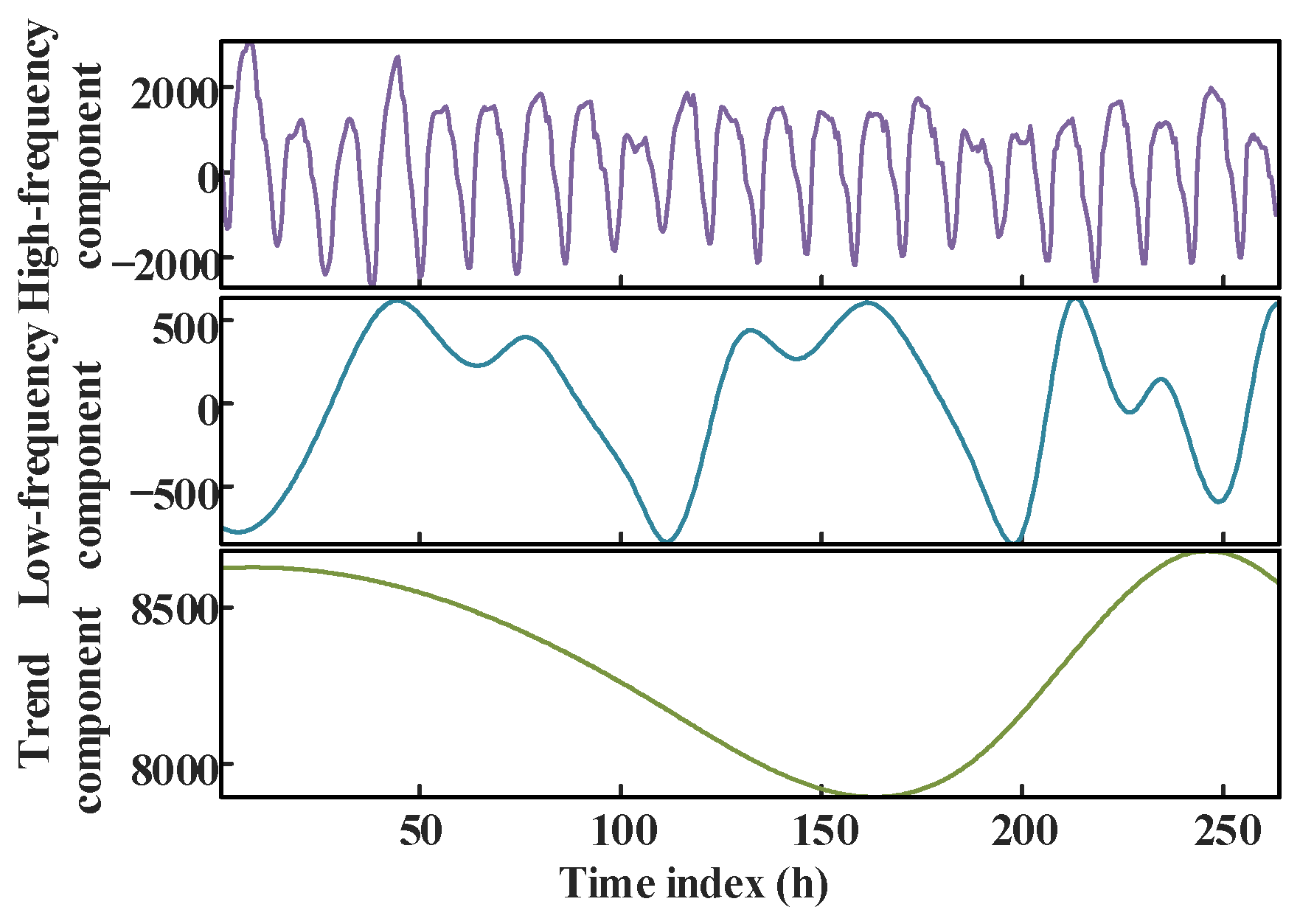
3.1. Load Sequence Decomposition Using CEEMDAN

The short-term load has strong randomness and poor regularity, so it needs to be smoothed to reduce the volatility. To improve the forecasting accuracy, the CEEMDAN is adopted to adaptively decompose the original load into multiple mode components with different frequency characteristics. By replacing the white noise with the IMF components and averaging the IMF components of each order as a whole, the CEEMDAN avoids mode mixing and solves the problem that the white noise is easy to transfer and difficult to eliminate [37]. The calculation steps of the CEEMDAN are as follows:
The white Gaussian noise is added to the original load time series.
y i ( t ) = y ( t ) + α ω i ( t ) , i = 1 , n
where yi(t) represents the sequence after adding the white Gaussian noise for the i-th time; α is the signal–noise ratio; ωi is the white Gaussian noise added for the i-th time; n is the number of noise additions.
The sequence yi(t) is decomposed by the EMD, and the first intrinsic model function IMF1(t) and residual R1(t) are obtained:
IMF 1 ( t ) = 1 n i = 1 n IMF 1 , i ( t ) R 1 ( t ) = y ( t ) IMF 1 ( t )
After adding the white Gaussian noise to the decomposed residual component, the EMD is continued.
IMF j ( t ) = 1 n i = 1 n E j ( R j 1 ( t ) + α j 1 E j 1 ( ω i ( t ) ) ) R j ( t ) = R j 1 IMF j ( t )
where IMFj represents the j-th mode component; E(.) represents the IMF component by the EMD; Rj is the j-th residual component; αj is the signal–noise ratio added to Rj.
The above step is repeated until R(t) becomes a monotone function and cannot be decomposed. Finally, the original load is expressed as the sum of H intrinsic model functions and a residual.
y ( t ) = i = 1 H IMF i ( t ) + R ( t )

3.2. Load Sequence Reconstruction Using PE

After decomposing the original load using the CEEMDAN, there are some problems, such as increased data dimension, reduced operating efficiency, and limited improvement in the accuracy [38,39]. To enhance the decomposition effect and reduce the complexity of the forecasting model, the PE criterion with a simple structure, fast calculation, and good anti-interference is used to evaluate the complexity of each sub-time series and reconstruct them into the high-frequency component, the low-frequency component, and the trend component. The calculation steps of the PE criterion are as follows:
The decomposed component sequence w(i) is spatially reconstructed.
W = w ( 1 ) w ( 1 + λ ) w ( 1 + ( m 1 ) λ ) w ( 2 ) w ( 2 + λ ) w ( 2 + ( m 1 ) λ )                  w ( l ) w ( l + λ ) w ( i + ( m 1 ) λ )
where λ is the delay time; l is the number of the reconstruction vectors; W is a matrix after space reconstruction; m is the embedding dimension.
The row vectors of the matrix W are arranged in ascending order.
w ( i + ( j 1 1 ) λ ) w ( i + ( j 2 1 ) λ ) w ( i + ( j m 1 ) λ )
where j is the index of the column of the m element in the new sequence.
Based on the formula of Shannon entropy, the normalized PE value HPE is shown as in Equation (13). The smaller the value, the more regular the corresponding time series.
H PE = ln ( m ! ) 1 j = 1 m ! D ( S j ) ln ( D ( S j ) )
where D is the occurrence probability of individual symbol sequences; Sj is the j-th symbol sequence.

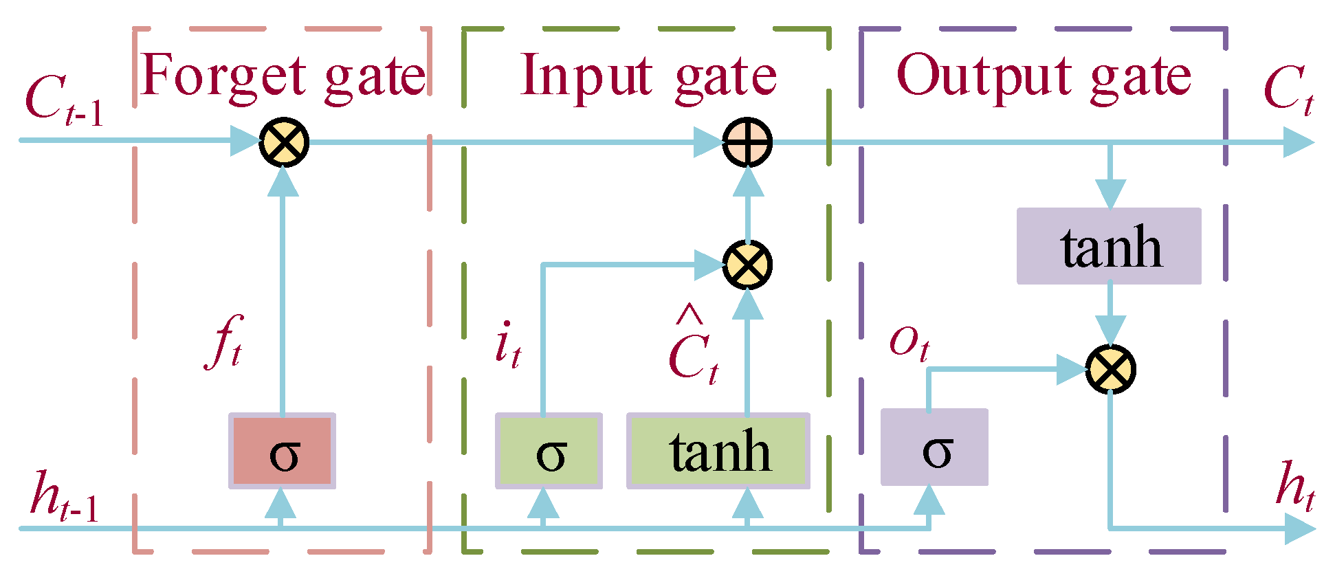
3.3. Load Forecast Using the Combined CNN-BILSTM Model

To fully tap the multi-dimensional feature of the original load data, a CNN-BILSTM model with strong nonlinear fitting ability is constructed by combining the advantages that the CNN network can capture the spatial features of the load time series and the BILSTM network can extract the bidirectional dependence of the load time series [40]. The structure of the CNN-BILSTM model is shown in Figure 3.
The CNN can capture the local dependence relationship of the load time series by adjusting the size and movement direction of the convolutional kernel and deeply explore the spatial features [26]. The CNN primarily consists of a convolutional layer, pooling layer, and other layers. The convolutional layer can perform the convolution operation on the load data.
T j L = f ( T j L 1 K j L + b j L )
where T j L is the j-th feature mapping of the L layer; f(·) is the activation function; b j L is the bias term; K j L is the convolutional kernel.
The pooling layer can reduce the feature dimension and prevent overfitting, and its computational formula is as follows:
T j L = f ( down ( T j L 1 + b j L ) )
where down(·) represents the down sampling function.
By adding the memory unit and gate mechanism, the LSTM addresses the problems of the vanishing and exploding gradient in traditional recurrent neural networks [28]. However, the LSTM only extracts the forward dependence relationship of the load time series, resulting in low data utilization. The structure of the LSTM network is shown in Figure 4.
The BILSTM adds back propagation on the basis of the forward propagation of the LSTM. Therefore, the BILSTM can perform bidirectional recursive feedback on both past and future states in the hidden layer; deeply explore the internal relationships among the current load, past, and future load data; and further improve the time series analysis ability and data utilization rate of the forecasting model [40]. The combination process of each hidden layer state in the BILSTM network is as follows:
h t = LSTM ( r t , h t 1 ) h i = LSTM ( r t , h i 1 ) h t = a t h t + b t h i + c t
where LSTM represents the operation process of the long short-term memory network; rt is the input at the current moment; ht and hi are the forward and backward hidden layer states, respectively; at and bt are the output weights of the forward and backward hidden layers, respectively; ct is the bias parameters of the hidden layer at the current moment.
Given that the load data extend solely along the time axis direction, this paper adopts a CNN consisting of two convolutional layers and one max pooling layer and uses a fixed-size sliding window to capture the data features. The data after pooling are input into the BILSTM network. To deeply mine the features of the load time series and prevent overfitting, this paper employs two BILST layers, two Dropout layers, and one fully connected layer that integrates the extracted features.

4. Combinative Forecasting Model Based on VAR and CEEMDAN-CNN-BILSTM

Based on the VAR model with multivariate input, the CEEMDAN-CNN-BILSTM model and SCSSA, this study proposes a short-term load forecasting method to enhance the forecasting accuracy. Compared to the traditional load forecasting methods, the proposed method takes into account the impact of multiple contributing factors on the load forecasting, introduces the CEEMDAN to decompose the original load data, and integrates the multivariate time series analysis ability of the mathematical statistics method with the nonlinear fitting advantage of the machine learning method. The specific steps are given below.
Step 1. Based on the Spearman correlation coefficient, contributing factors strongly correlated with the short-term load are extracted from many factors. The autocorrelation function (ACF) analysis, the partial autocorrelation function (PACF) analysis, and the augmented Dickey–Fully (ADF) test are performed to determine the stationarity of each time series.
Step 2. A VAR model with multivariate input is built, and the Levenberg–Marquardt algorithm is introduced to estimate the parameters, realizing the regression forecasting analysis of the load time series.
Step 3. Based on the CEEMDAN with PE, the original load time series is adaptively decomposed and reconstructed into multiple relatively stationary mode components to reduce its randomness and volatility.
Step 4. A CNN-BILSTM model with strong nonlinear fitting ability is structured, and each mode component is input into the model for forecasting.
Step 5. The SCSSA is adopted to optimize the parameters of the combinative model to further improve the forecasting accuracy of the short-term load.

4.1. Optimiztion of the Combinative Forecasting Model Using SCSSA

The hyperparameters are important factors that determine the performance of the forecasting model, including the number of neurons in the hidden layer, the learning rate, and the regularization parameter. The main factors that affect the performance of the forecasting model are the learning rate and the number of neurons in the hidden layer. If the number of neurons in the hidden layer is too large or too small, the error of the prediction result will increase. The learning rate determines the parameter update speed of the BILSTM model, thus determining whether the optimal value can be achieved. To give full attention to the combined advantages of the mathematical statistics method and machine learning method, the SCSSA is adopted to constantly update those parameters in the proposed model until the optimal solution is found. The SCSSA introduces the sine–cosine strategy and the Cauchy mutation strategy into the updated formulas of the discoverer and follower, respectively, which solves the problem that the conventional sparrow search algorithm easily falls into the local optimum and lacks the global search ability [41,42].
The new updated formula for the discoverer location is as follows:
Z i , j t + 1 = σ Z i , j t + β 1 sin β 2 | β 3 Z b e s t Z i , j t | , δ < S T σ Z i , j t + β 1 cos β 2 | β 3 Z b e s t Z i , j t | , δ S T
where Zi,j represents the position of the i-th sparrow in the j-th dimension; t is the current number of iterations; Zbest represents the optimal position; σ is the nonlinear weighting factor; β1 is the step search factor; β2 and β3 are random numbers between 0 and 2π.
The new updated formula for the follower location is as follows:
Z i , j t + 1 = Z b e s t ( t ) + cauchy ( 0 , 1 ) Z b e s t ( t )
where ⊗ stands for an element-wise multiplication; cauchy(0,1) is the standard Cauchy distribution function.
The step search factor of the sine–cosine algorithm exhibits a linearly decreasing trend, which will affect the balance between the global search and local development of the SSA. Consequently, this factor is modified to a nonlinear weight factor to reduce the dependence of the individual position update on the current solution.
β 1 = e t t max 1 e 1
where e is a natural constant; tmax is the maximum number of iterations.
The refracted opposition-based learning mechanism is adopted to initialize the population position.
Z i , j = ( χ j + ψ j ) 2 + ( χ j + ψ j ) 2 g + Z i , j g
where χj and ψj are the minimum and maximum values of the j-th position, respectively; Z i , j is the reverse refraction position of Zi,j; g is a scaling factor.

4.2. Evaluation Indicators

To verify the effectiveness and accuracy of the proposed combinative model, the root mean square error (ERMSE), the mean absolute percentage error (EMAPE), the mean absolute error (EMAE), and the R-squared (R2) are used as the evaluation indicators of the forecasting model. The calculation formulas are as follows:
E R M S E = 1 Q q = 1 Q P q pred P q real 2
E M A P E = 1 Q q = 1 Q | P q pred P q pred P q real | × 100 %
E MAE = 1 Q q = 1 Q | P q pred P q real |
R 2 = 1 q = 1 Q P q pred P q real 2 q = 1 Q P q pred P q aver 2
where P q p r e d and P q real represent the predicted and true values of the q-th sample point in the text set, respectively; Q is the sample size; P q aver is the simple mean.

5. Numerical Analysis

The actual load data (including the dry bulb temperature, dew point temperature, humidity, real-time electricity price, and power load) from 6 March 2006 to 31 March 2006 in Australia are collected [43], and the sampling interval is 1 h. The data from 6 March to 31 March are used as the training set, while the data from 30 March to 31 March are used as the test set.

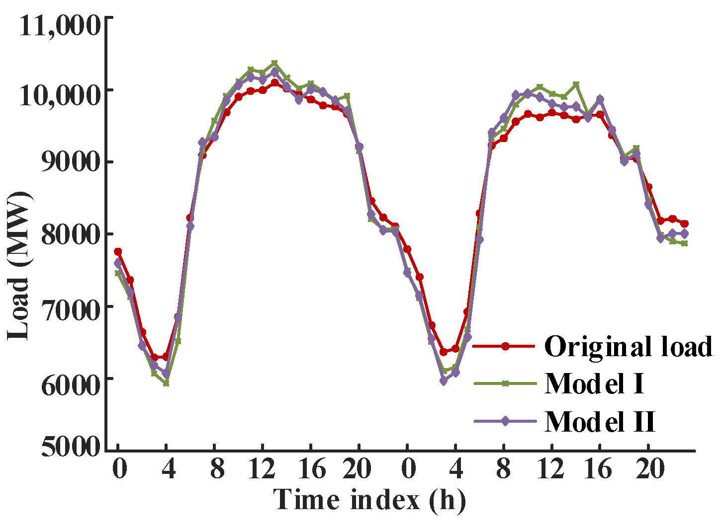
5.1. Forecasting Analysis of the AVR Model with Multivariate Input

The Spearman correlation coefficient is adopted to evaluate the correlation between the short-term load and contributing multiple factors, as illustrated in Figure 5. It can be observed from Figure 5 that the real-time electricity price and dry bulb temperature have a strong correlation with the load data, as the correlation coefficients are greater than 0.5. In contrast, the Spearman correlation coefficients for the dew point temperature and humidity are smaller than 0.4 and show weak correlations with the load data. Consequently, the forecasting model should incorporate the real-time electricity price and dry bulb temperature as key input variables while excluding the dew point temperature and humidity due to the insufficient correlation with the load data.
These time series of the load, real-time electricity price, and dry bulb temperature are analyzed by the ACF and PACF. It is observed that the ACFs of the above time series have the tailing characteristic, and the PACFs have the truncating characteristic, which meet the conditions for constructing a VAR model. To avoid spurious regression, the VAR model requires that all time series involved in modeling must be stationary. Consequently, the ADF test is adopted to assess the stationarity of these time series of load, price, and dry bulb temperature, and the results are summarized in Table 2, where 0 indicates non-stationarity and 1 indicates stationarity.
It is observed that these time series of the load, real-time electricity price, and dry bulb temperature are non-stationary under the original order, but they tend to be stationary after taking the first-order difference, as illustrated in Figure 6. Therefore, a first-order differential VAR model with multivariate variables will be established. Based on the Akaike information criterion, the optimal model order is determined to be 7.
To investigate the impact of multiple contributing factors on load forecasting, the proposed VAR model is compared with the VAR model with only a single factor, and the forecasting results are illustrated in Figure 7, and the evaluation indicators are given in Table 3. Model I represents the VAR model that takes the time series of the load and temperature as the input variables, while model II represents the VAR model that takes the time series of the load, real-time electricity price, and dry bulb temperature as the input variables of the forecasting model.
As illustrated in Figure 7 and Table 3, model I inadequately accounts for the impact of multiple factors on load forecasting, and its forecasting accuracy is poor, especially when the load trend changes. In contrast, the proposed algorithm in this paper selects multiple contributing factors strongly correlated with the short-term load based on the Spearman correlation coefficient and establishes a VAR model with multiple variables. This method results in a reduction in the ERMSE, EMAPE, and EMAE by 15.17%, 18.01%, and 19.12%, respectively, and obtains a higher forecasting accuracy.

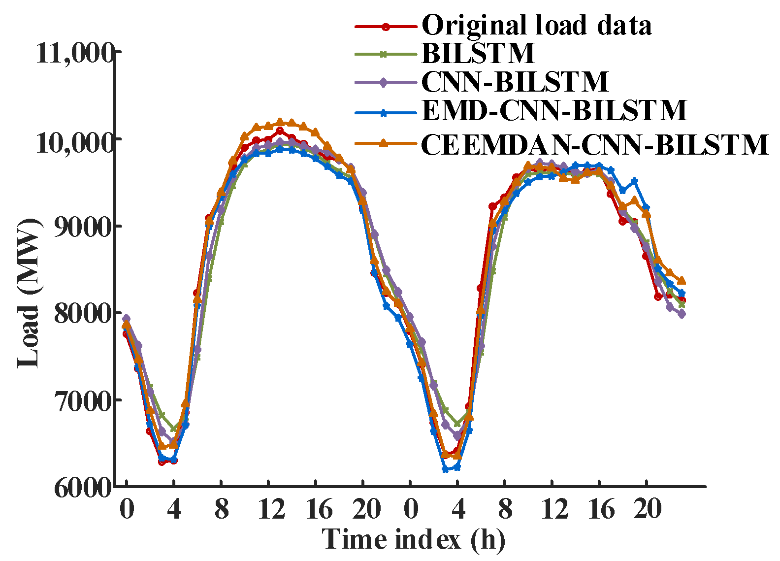
5.2. Forecasting Analysis of the CEEMDAN-CNN-BILSTM Model

The noise standard deviation is set to 0.2, the number of noise additions is set to 50, and the maximum number of iterations is set to 200. The load time series is adaptively decomposed into the ten IMF components, with frequencies ranging from high to low. Each component represents distinct frequency features of the load data, as illustrated in Figure 8. This decomposition has effectively reduced the volatility and noise in the original load data.
Directly forecasting these decomposed components will lead to a significant increase in the computational scale. To reduce the complexity of the forecasting model and improve the training efficiency, the PE criterion is used to assess the complexity of each component, followed by data reconstruction, as summarized in Table 4. The entropy values of IMF1~IMF4 are more than 0.9, indicating strong randomness and volatility, and these components are thus reconstructed as high-frequency components. IMF5 and IMF7 have similar entropy values, reflecting the local fluctuation features of the load time series, and these components are thus reconstructed as low-frequency components. IMF8~IMF10 are relatively smooth, roughly reflecting the overall trend of the load time series, and these components are thus reconstructed as the trend components. The reconstructed component waveform is shown in Figure 9. The number of computations required for the forecasting model is reduced from 10 to 3, and the majority of the detailed features of the original components are retained.
The forecasting results of the proposed CEEMDAN-CNN-BILSTM model are compared to those of the BILSTM, CNN-BILSTM, and EMD-CNN-BILSTM models to prove their superiority. The forecasting results are shown in Figure 10, and the evaluation indicators are given in Table 5. The presentation and comparison of the experimental results focus on the overall output performance, and the forecasting accuracy of each component is no longer analyzed.
As illustrated in Figure 10 and Table 5, compared to the BILSTM model, the CNN-BILSTM model enhances the ability to capture the local features of the load time series, and its ERMSE and EMAE have decreased by 18.90% and 15.01%, respectively. Given that the short-term load is impacted by many external factors and has randomness and volatility, the direct forecasting method is difficult to forecast accurately. By using a “decomposition–reconstruction–forecasting” strategy and constructing the CNN-BILSTM model for each component after decomposition and reconstruction, the non-stationarity and complexity of the load data can be effectively reduced. Compared to the EMD, the CEEMDAN addresses the problem of mode mixing. This leads to reductions in the ERMSE, EMAPE, and EMAE by 17.48%, 19.98%, and 21.38%, respectively, while the R2 increases by 0.80%.

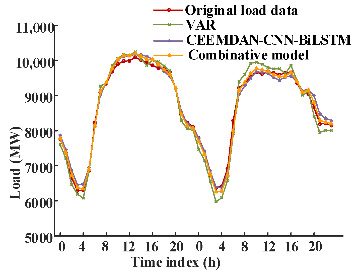
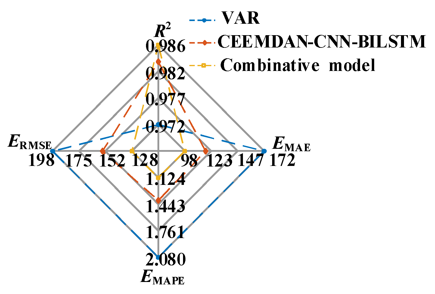
5.3. Forecasting Analysis of the Combinative Model

Taking ERMSE as the optimization goal, the SCSSA is used to optimize the parameters of the combinative forecasting model. The population number is set as 20, the discoverer ratio is set as 0.2, the maximum number of iterations is set as 50, the safety threshold is set as 0.7, the initial learning rate is set as 0.002, the initial regularization parameter is set as 0.01, and the initial numbers of neurons in the hidden layer are set as 3 and 5, respectively. To enhance the population diversity, the refracted opposition-based learning mechanism is used to initialize the population position.
To verify the performance of the combinative forecasting model established in this paper, it is compared to the VAR model and the CEEMDAN-CNN-BILSTM model. The forecasting results are illustrated in Figure 11, and the evaluation indicators are shown in Figure 12. Compared to the CEEMDAN-CNN-BILSTM model, the proposed algorithm not only reduces the volatility and randomness of the load data but also takes into account the impact of multiple contributing factors on the load forecasting. This leads to reductions in the ERMSE, EMAPE, and EMAE by 16.81%, 19.44%, and 16.48%, respectively, while the R2 increases by 0.30%. The combinative model optimized by the SCSSA integrates the multivariate time series analysis ability of the mathematical statistics method and the nonlinear fitting advantage of the machine learning method, thereby effectively improving the forecasting accuracy.

6. Conclusions

Aiming at the problem that the short-term load is affected by many factors and has strong nonlinearity and volatility, which increases the forecasting difficulty, this paper proposes a short-term load forecasting method considering multiple contributing factors based on VAR and CEEMDAN-CNN-BILSTM. This approach not only takes account of the impact of multiple contributing factors on load forecasting but also reduces the volatility and randomness of the load data. Based on the actual load data, the following conclusions are drawn:
(1)
Based on the Spearman correlation coefficient, the multiple contributing factors strongly correlated with the short-term load are selected, and the improved VAR model with multi-variable input is derived, which can improve the forecasting accuracy.
(2)
In comparison with the single machine learning model, the original load data are decomposed and reconstructed into multiple relatively stationary mode components by combining the CEEMDAN and PE criteria, which can effectively reduce its volatility and randomness and facilitate the CNN-BILSTM model to extract its features. Compared to the EMD, the ERMSE, EMAPE, and EMAE are decreased by 16.81%, 19.44%, and 16.48%, respectively, while the R2 is increased by 0.30%.
(3)
The combinative forecasting model based on improved VAR and CEEMDAN- CNN-BILSTM integrates the multivariate time series analysis ability of the mathematical statistics method with the nonlinear fitting advantage of the machine learning method. The proposed method not only considers the impact of multiple contributing factors on the load forecasting but also reduces the volatility and randomness of the short-term load data, effectively improving the accuracy of the short-term load forecasting model.
(4)
The error correction is not considered in this paper. A support vector regression model can be introduced in a follow-up study to construct the corrected error sequence and compensate for the initial forecasting sequence so as to further improve the forecasting accuracy.

Author Contributions

Conceptualization and funding acquisition: B.W., L.W., Y.M., D.H. and S.L. Validation, writing—original draft, writing—review and editing, resources and software, and data curation: B.W., Y.M., W.S. and S.L. All authors have read and agreed to the published version of the manuscript.

Funding

This research was funded by the State Grid Anhui Economic and Technical Research Institute under grant B61209240017.

Data Availability Statement

The original contributions presented in this study are included in this article. Further inquiries can be directed at the corresponding author.

Conflicts of Interest

All the authors declare that the research was conducted in the absence of any commercial or financial relationships that could be construed as a potential conflict of interests.

References

  1. Rubasinghe, O.; Zhang, X.; Chau, T.K.; Chow, Y.H.; Fernando, T.; Iu, H.H.-C. A novel sequence to sequence data modelling based CNN-LSTM algorithm for three years ahead monthly peak load forecasting. IEEE Trans. Power Syst. 2024, 39, 1932–1947. [Google Scholar] [CrossRef]
  2. Voumik, L.C.; Islam, M.A.; Ray, S.; Mohamed Yusop, N.Y.; Ridzuan, A.R. CO2 emissions from renewable and non-renewable electricity generation sources in the G7 countries: Static and dynamic panel assessment. Energies 2023, 16, 1044. [Google Scholar] [CrossRef]
  3. Li, S.; Ye, J. EEOP-based interaction path differentiation and control parameter optimization to mitigate oscillation in multi-DFIG wind farm. IEEE Trans. Power Syst. 2024, 39, 7403–7416. [Google Scholar] [CrossRef]
  4. Sun, J.; Peng, Y.; Ni, Y.; Wei, w.; Cai, T.; Xi, W. Power load forecasting method based on improved federated learning algorithm. High Volt. Eng. 2024, 50, 3039–3049. [Google Scholar]
  5. Hua, Q.; Fan, Z.; Mu, W.; Cui, J.; Xing, R.; Liu, H.; Gao, J. A short-term power load forecasting method using CNN-GRU with an attention mechanism. Energies 2025, 18, 106. [Google Scholar]
  6. Zhou, B.; Zhang, Z.; Li, G.; Yang, D.; Santos, M. Review of key technologies for offshore floating wind power generation. Energies 2023, 16, 710. [Google Scholar] [CrossRef]
  7. Feng, P.; Xu, J.; Wang, Z.; Li, S.; Shen, Y.; Gui, X. Impact of phase angle jump on a doubly fed induction generator under low-voltage ride-through based on transfer function decomposition. Energies 2024, 17, 4778. [Google Scholar] [CrossRef]
  8. Wei, N.; Yin, C.; Yin, L.; Tan, J.; Liu, J.; Wang, S.; Qiao, W.; Zeng, F. Short-term load forecasting based on WM algorithm and transfer learning model. Appl. Energy 2024, 353, 122087. [Google Scholar] [CrossRef]
  9. Hu, W.; Zhang, X.; Li, Z.; Li, Q.; Wang, H. Short-term load forecasting based on an optimized VMD-mRMR-LSTM model. Power Syst. Prot. Control 2022, 50, 88–97. [Google Scholar]
  10. Xu, J.; Feng, P.; Gong, J.; Jiang, G.; Li, S.; Gui, X. LVRT control strategy of GSC passive sliding mode control for doubly-fed wind turbine. In Proceedings of the 2024 6th International Conference on Energy Systems and Electrical Power (ICESEP), Wuhan, China, 21–23 June 2024; pp. 573–576. [Google Scholar]
  11. Masood, Z.; Gantassi, R.; Choi, Y. Enhancing short-term electric load forecasting for households using quantile LSTM and clustering-based probabilistic approach. IEEE Access 2024, 12, 77257–77268. [Google Scholar]
  12. Liu, J.; Cong, L.; Xia, Y.; Pan, G.; Zhao, H.; Han, Z. Short-term power load prediction based on DBO-VMD and an IWOA-BILSTM neural network combination model. Power Syst. Prot. Control 2024, 52, 123–133. [Google Scholar]
  13. Sias, Q.A.; Gantassi, R.; Choi, Y.; Bae, J.H. Recurrence multilinear regression technique for improving accuracy of energy prediction in power systems. Energies 2024, 17, 5186. [Google Scholar] [CrossRef]
  14. ElMenshawy, M.S.; Massoud, A.M. Short-term load forecasting in active distribution networks using forgetting factor adaptive extended kalman filter. IEEE Access 2023, 11, 103916–103924. [Google Scholar] [CrossRef]
  15. Guo, M.; Hao, Y.; Lee, K.Y.; Sun, L. Extended-state Kalman filter-based model predictive control and energy-saving performance analysis of a coal-fired power plant. Energy 2025, 314, 134169. [Google Scholar]
  16. Xie, Y.; Jin, M.; Zou, Z.; Xu, G.; Feng, D.; Liu, W. Real-time prediction of Docker container resource load based on a hybrid model of ARIMA and triple exponential smoothing. IEEE Trans. Cloud Comput. 2022, 10, 1386–1401. [Google Scholar] [CrossRef]
  17. Hora, C.; Dan, F.C.; Bendea, G.; Secui, C. Residential short-term load forecasting during atypical consumption behavior. Energies 2022, 15, 291. [Google Scholar] [CrossRef]
  18. Jeong, D.; Park, C.; Ko, Y.M. Short-term electric load forecasting for buildings using logistic mixture vector autoregressive model with curve registration. Appl. Energy 2021, 282, 116249. [Google Scholar]
  19. Wang, Z.; Ku, Y.; Liu, J. The power load forecasting model of combined SaDE-ELM and FA-CAWOA-SVM based on CSSA. IEEE Access 2024, 12, 41870–41882. [Google Scholar]
  20. Wu, J.; Wang, Y.; Tian, Y.; Burrage, K.; Cao, T. Support vector regression with asymmetric loss for optimal electric load forecasting. Energy 2021, 223, 119969. [Google Scholar]
  21. Shern, S.J.; Sarker, M.T.; Haram, M.H.S.M.; Ramasamy, G.; Thiagarajah, S.P.; Al Farid, F. Artificial intelligence optimization for user prediction and efficient energy distribution in electric vehicle smart charging systems. Energies 2024, 17, 5772. [Google Scholar] [CrossRef]
  22. Aprillia, H.; Yang, H.-T.; Huang, C.-M. Statistical load forecasting using optimal quantile regression random forest and risk assessment index. IEEE Trans. Smart Grid 2021, 12, 1467–1480. [Google Scholar]
  23. Zulfiqar, M.; Gamage, K.A.A.; Rasheed, M.B.; Gould, C. Optimised deep learning for time-critical load forecasting using LSTM and modified particle swarm optimisation. Energies 2024, 17, 5524. [Google Scholar] [CrossRef]
  24. Kong, W.; Dong, Z.; Jia, Y.; Hill, D.J.; Xu, Y.; Zhang, Y. Short-term residential load forecasting based on LSTM recurrent neural network. IEEE Trans. Smart Grid 2019, 10, 841–851. [Google Scholar]
  25. Wang, F.; Liu, Z. Power load prediction based on IGWO-BILSTM network. Math. Prob. Eng. 2023, 2023, 8996138. [Google Scholar]
  26. Ouyang, F.; Wang, J.; Zhou, H. Short-term power load forecasting method based on improved hierarchical transfer learning and multi-scale CNN-BILSTM-Attention. Power Syst. Prot. Control 2023, 51, 132–140. [Google Scholar]
  27. Chen, K.; Chen, K.; Wang, Q.; He, Z.; Hu, J.; He, J. Short-term load forecasting with deep residual networks. IEEE Trans. Smart Grid 2019, 10, 3943–3952. [Google Scholar]
  28. Shi, Z.; Ran, Q.; Xu, F. Short-term load forecasting based on aggregated secondary decomposition and informer. Power Syst. Technol. 2024, 48, 2574–2583. [Google Scholar]
  29. Mounir, N.; Ouadi, H.; Jrhilifa, I. Short-term electric load forecasting using an EMD-BI-LSTM approach for smart grid energy management system. Energy Build. 2023, 288, 113022. [Google Scholar]
  30. Wen, Y.; Pan, S.; Li, X.; Li, Z. Highly fluctuating short-term load forecasting based on improved secondary decomposition and optimized VMD. Sustain. Energy Grids Netw. 2024, 37, 101270. [Google Scholar]
  31. Hou, R.; Liu, J.; Zhao, J.; Liu, J.; Chen, W. State of charge balancing control strategy for wind power hybrid energy storage based on successive variational mode decomposition and multi-fuzzy control. Energies 2024, 17, 5650. [Google Scholar] [CrossRef]
  32. Ran, P.; Dong, K.; Liu, X.; Wang, J. Short-term load forecasting based on CEEMDAN and Transformer. Electr. Power Syst. Res. 2023, 214, 108885. [Google Scholar]
  33. Gopali, S.; Siami-Namini, S.; Abri, F.; Namin, A.S. A comparative multivariate analysis of VAR and deep learning-based models for forecasting volatile time series data. IEEE Access 2024, 12, 155423–155436. [Google Scholar]
  34. Shang, N.; Lu, Z.; Chen, Z.; Wang, Y.; Wen, F. Empirical analysis of electricity and carbon price correlation based on VARM and copula. Power Syst. Technol. 2023, 47, 2305–2317. [Google Scholar]
  35. Liu, R.; Li, L. Parameter extraction for energetic hysteresis model based on the hybrid algorithm of simulated annealing and Levenberg-Marquardt. Proc. CSEE 2019, 39, 875–884+966. [Google Scholar]
  36. Long, Q.; Yu, H.; Xie, F.; Lu, N.; Lubkeman, D. Diesel generator model parameterization for microgrid simulation using hybrid box-constrained Levenberg-Marquardt algorithm. IEEE Trans. Smart Grid 2021, 12, 943–952. [Google Scholar]
  37. Liu, H.; Li, Z.; Li, C.; Shao, L.; Li, J. Research and application of short-term load forecasting based on CEEMDAN-LSTM modeling. Energy Rep. 2024, 12, 2144–2155. [Google Scholar]
  38. Hua, H.; Zhu, Y. Short-term Load forecasting based on CEEMDAN PE-GWO-LSTM. In Proceedings of the 2023 3rd International Conference on Energy Engineering and Power Systems (EEPS), Dali, China, 28–30 July 2023; pp. 1096–1101. [Google Scholar]
  39. Chang, Y.; Yang, Z.; Pan, F.; Tang, Y.; Huang, W. Ultra-short-term wind power prediction based on CEEMDAN-PE-WPD and multi-objective optimization. Power Syst. Technol. 2023, 47, 5015–5026. [Google Scholar]
  40. Hu, X.; Li, H.; Si, C. Improved composite model using metaheuristic optimization algorithm for short-term power load forecasting. Electr. Power Syst. Res. 2025, 241, 111330. [Google Scholar]
  41. Li, S.; Tao, D. Optimization to controllability measure of the POD in DFIG-integrated power systems to improve small-signal stability margin considering the impact of pre-fault slip. Electr. Eng. 2024, 106, 5937–5952. [Google Scholar]
  42. Lv, Q.; Zhang, K.; Wu, X.; Li, Q. Fault diagnosis method of bearings based on SCSSA-VMD-MCKD. Processes 2024, 12, 1484. [Google Scholar] [CrossRef]
  43. Fan, X.; Li, Y. Short-term power load forecasting based on improved Autoformer model. Electr. Power Autom. Equip. 2024, 44, 171–177. [Google Scholar]
Figure 1. Multiple contributing factors to load forecasting.
Energies 18 01855 g001
Figure 2. Structure of the combination forecasting model.
Energies 18 01855 g002
Figure 3. Structure of the CNN-BILSTM.
Energies 18 01855 g003
Figure 4. Structure of the LSTM.
Energies 18 01855 g004
Figure 5. Heat map of the Spearman correlation coefficient.
Energies 18 01855 g005
Figure 6. Time series after the first-order difference.
Energies 18 01855 g006
Figure 7. Comparison of the forecasting results of two VAR models.
Energies 18 01855 g007
Figure 8. Results of the CEEMDAN decomposition.
Energies 18 01855 g008
Figure 9. Results of the component reconstruction.
Energies 18 01855 g009
Figure 10. Comparison of forecasting results of each model.
Energies 18 01855 g010
Figure 11. Forecasting results of the combinative model.
Energies 18 01855 g011
Figure 12. Evaluation indicators of the combinative model.
Energies 18 01855 g012
Table 1. Comparison of different references.
ReferenceModelTime ScaleAdvantageLimitation
[24]LSTM30 minsolve the gradient explosion problemlow data utilization
[25]IGWO-BILSTM1 hbidirectional recursive feedbackweak global search ability
[29]EMD-BILSTM1 hreduce the volatility and randomness of load datamode mixing
[30]VMD-LSTM1 hsolve mode mixingdifficultly parameter selection
[32]CEEMDAN-SE-TR1 hstrong adaptabilityincreased data dimension and calculating work
Table 2. Stationarity test results of the time series.
Time SeriesADF Test
[Load, Price, Dry bulb temperature][0, 0, 0]
[Load, Price, Dry bulb temperature][1, 1, 1]
Table 3. Evaluation indicators of two VAR models.
Forecasting ModelERMSE (MW)EMAPE (%)EMAE (MW)R2
Model I233.9792.537212.2080.96163
Model II198.49482.0801171.62350.97239
Table 4. Entropy calculation and reconstruction of each component.
ComponentIMF1IMF2IMF3IMF4IMF5
Entropy value0.99630.96690.95970.96470.7441
reconstructionHigh frequency componentLow
ComponentIMF6IMF7IMF8IMF9IMF10
Entropy value0.71480.70500.49610.49110.3139
reconstructionfrequency componentTrend component
Table 5. Evaluation indicators of each model.
Forecasting ModelERMSE (MW)EMAPE (%)EMAE (MW)R2
BILSTM295.30012.5976208.32230.93888
CNN-BILSTM239.49212.2267177.05200.95982
EMD-CNN
-BILSTM
186.86671.7440149.42680.97553
CEEMDAN-CNN
-BILSTM
154.21011.3956117.47440.98333
Disclaimer/Publisher’s Note: The statements, opinions and data contained in all publications are solely those of the individual author(s) and contributor(s) and not of MDPI and/or the editor(s). MDPI and/or the editor(s) disclaim responsibility for any injury to people or property resulting from any ideas, methods, instructions or products referred to in the content.

