
Multi-Energy Static Modeling Approaches: A Critical Overview


Abstract
1. Introduction
2. Energy Carriers Static Modeling Approaches
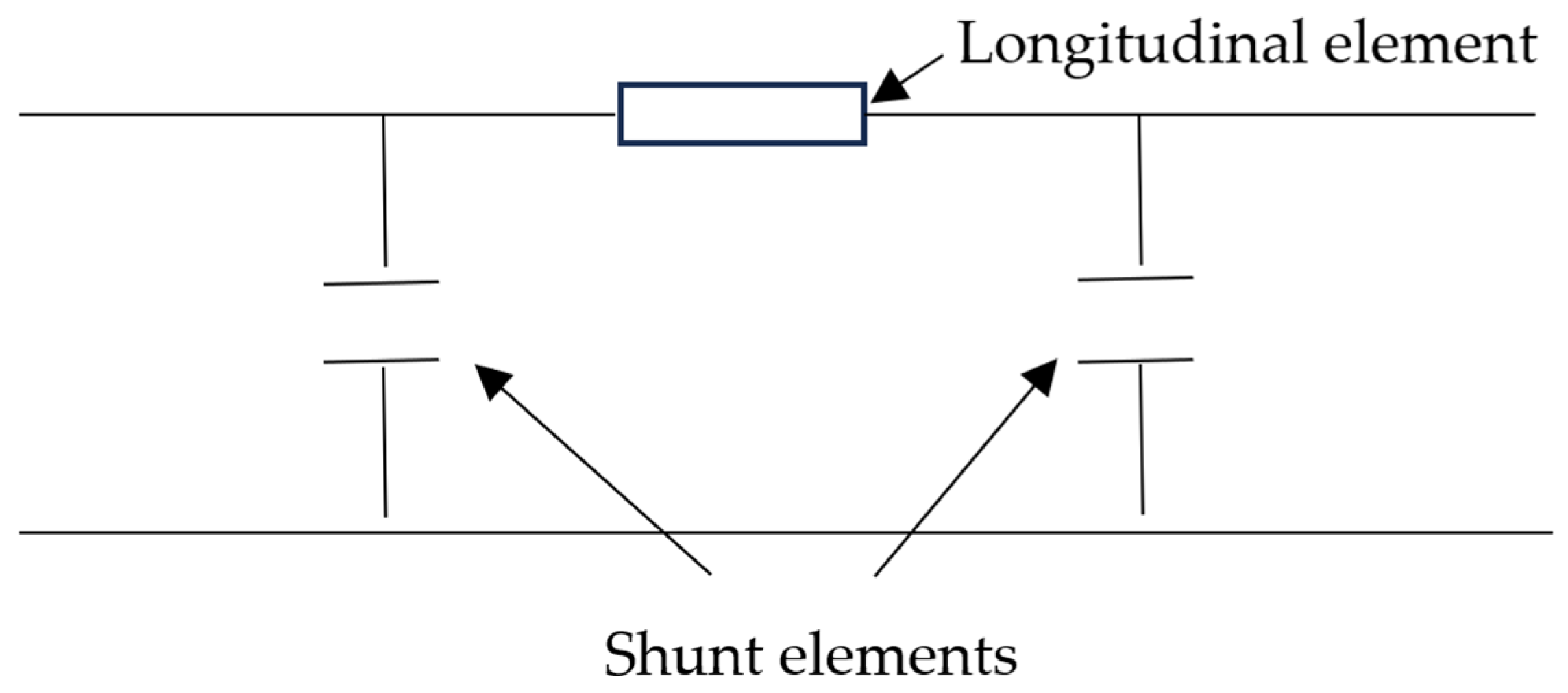
2.1. Electricity Networks Modeling
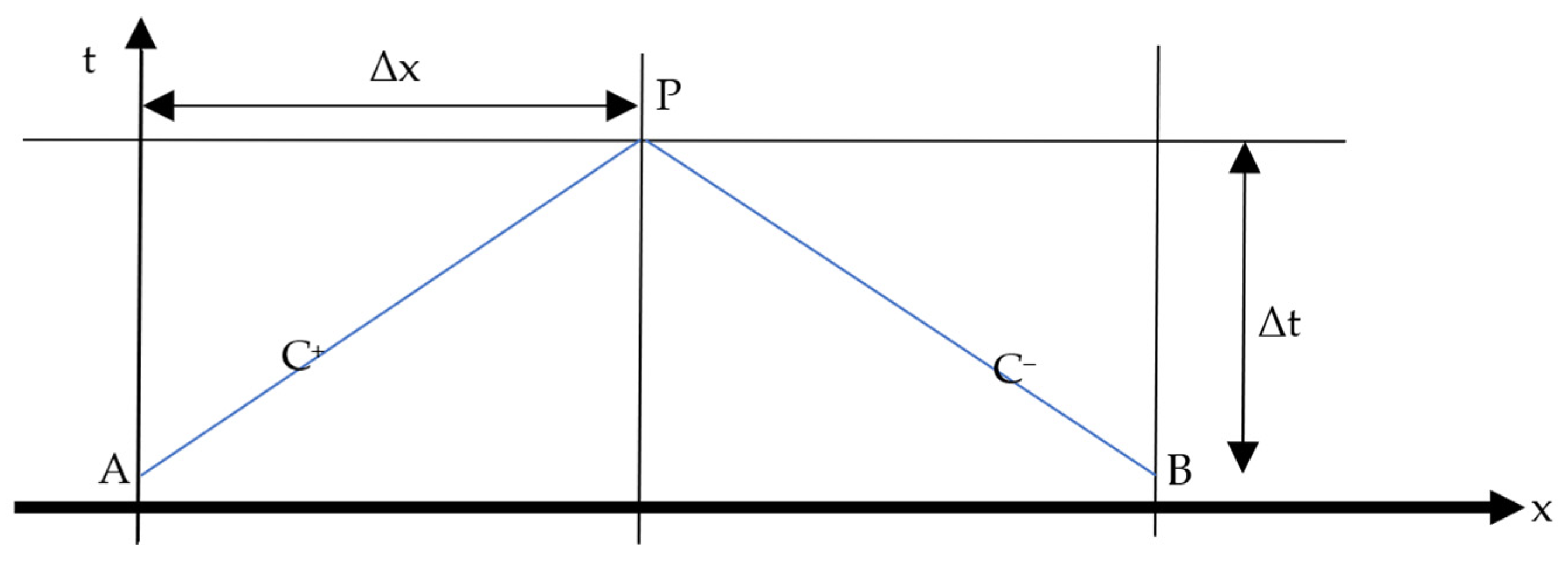
2.2. Compressible Fluids Modelling
- Turbulent motion in the pipeline (this is always verified for gas transport pipelines at a distance equal to some multiples of the diameter from the beginning and from the end of the duct). This allows us to adopt a mono-dimensional description for the fluid motion equations (otherwise, the Navier–Stokes [33] fluid dynamics laws should be used);
- The pipeline is regular—there are neither changes of section along x nor sharp changes of direction (curves). Such cases are usually modeled through concentrated losses (i.e., a pressure reduction proportional to the square of the fluid speed through a coefficient depending on the type of irregularity);
- The perfect gas law holds, stating that
- W(x) = constant, i.e., mass flow rate constant throughout the pipeline;
- The expression for pressure drops calculation:
2.3. Heat Networks Modeling
- The Weymouth Equation (12), describing pressure drops in the pipeline. It has the same formulation as for compressible fluids (additionally, as for gas pipelines, mass flow rate is constant under steady-state conditions);
- An equation describing heat propagation along the pipeline—this equation can be written, by considering an infinitesimal volume along the pipeline (see Figure 5), as
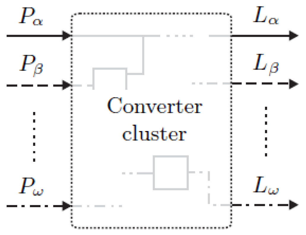
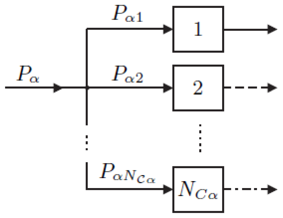
3. Typical ME Approaches
- c—energy carrier
- s—probabilistic scenario of RES production and load, and is the probability associated to each single scenario
- y—time horizon considered for the planning problem (typically a few years or decades, see e.g., [45] where three decades are considered—2030, 2040 and 2050)
- t—time horizon considered to calculate the system dispatch (e.g., one year)
- i—index enumerating each equipment in the system (e.g., electric lines). is the generic equipment item, and the integer variable associated with its investment.
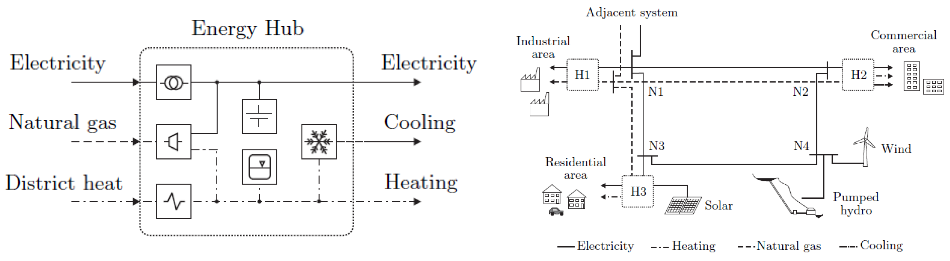
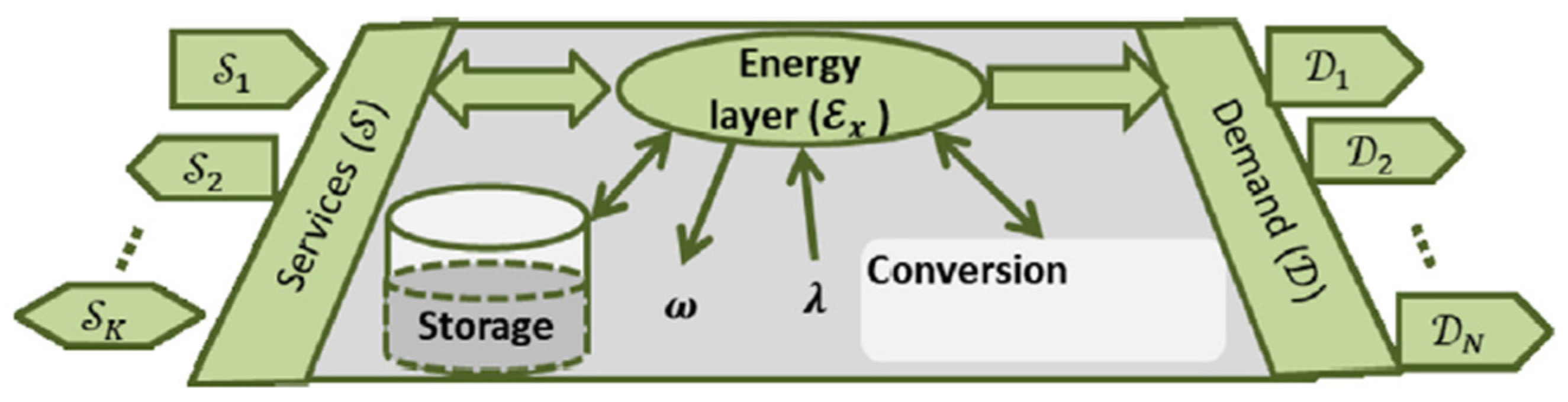
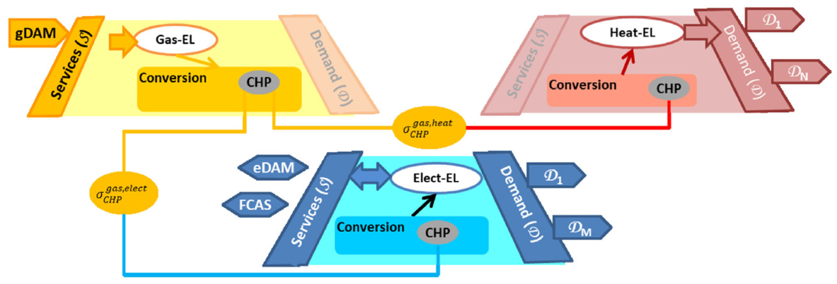
3.1. Energy Hub Representation
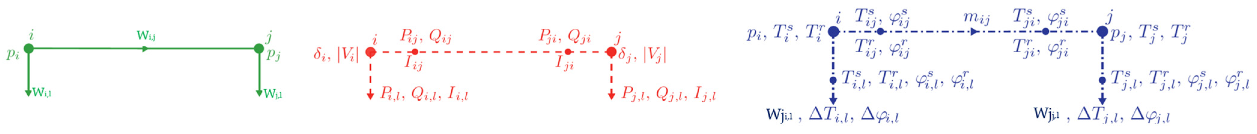
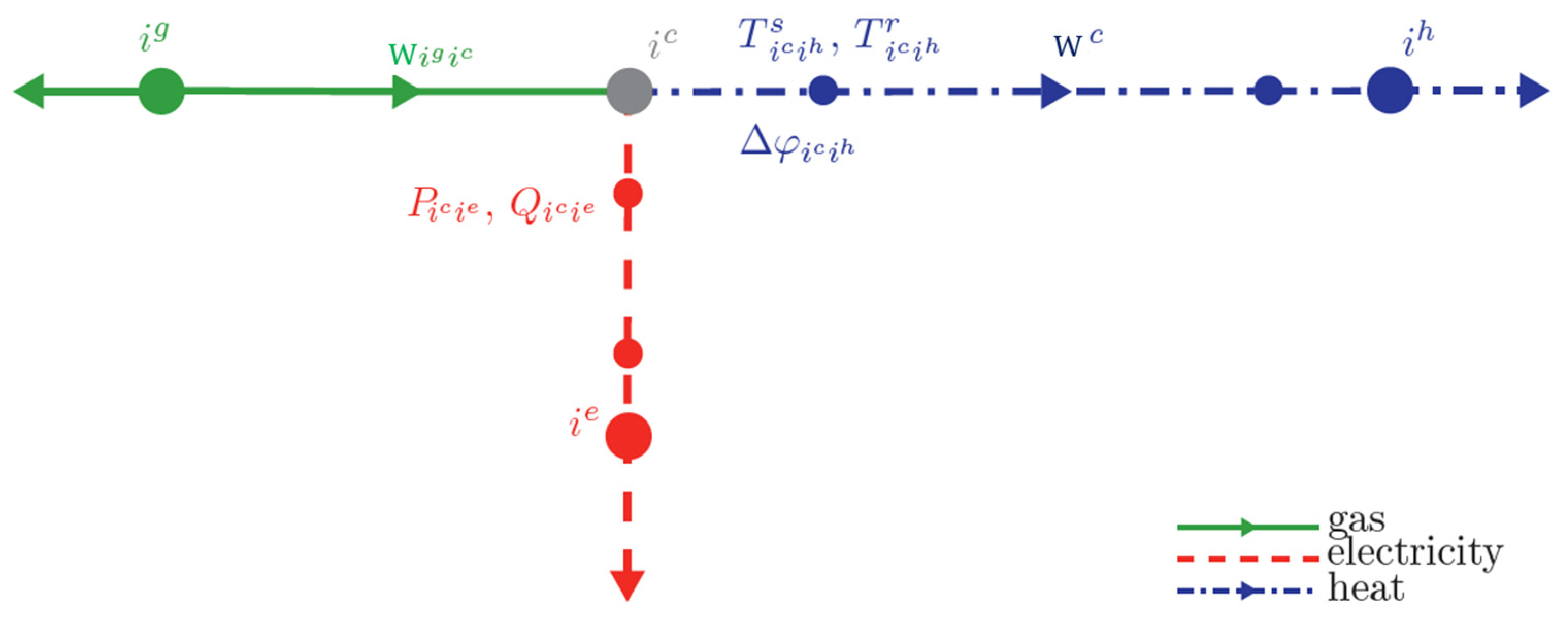
3.2. Graph Representation
- First law—conservation of mass or energy for each node;
- Second law—the sum of potential differences over each loop is zero.
- Green color for gas networks. Variables: pressures (p) and mass flow rates (W);
- Red color for electricity networks. Variables: active powers (P), reactive powers (Q), voltages (V), angles (δ), currents (I);
- Blue color for heat networks (the return line is not explicitly represented). Variables: pressures (p), thermal flows (φ), supply temperature (Ts) return temperature (Tr), water flows (W).
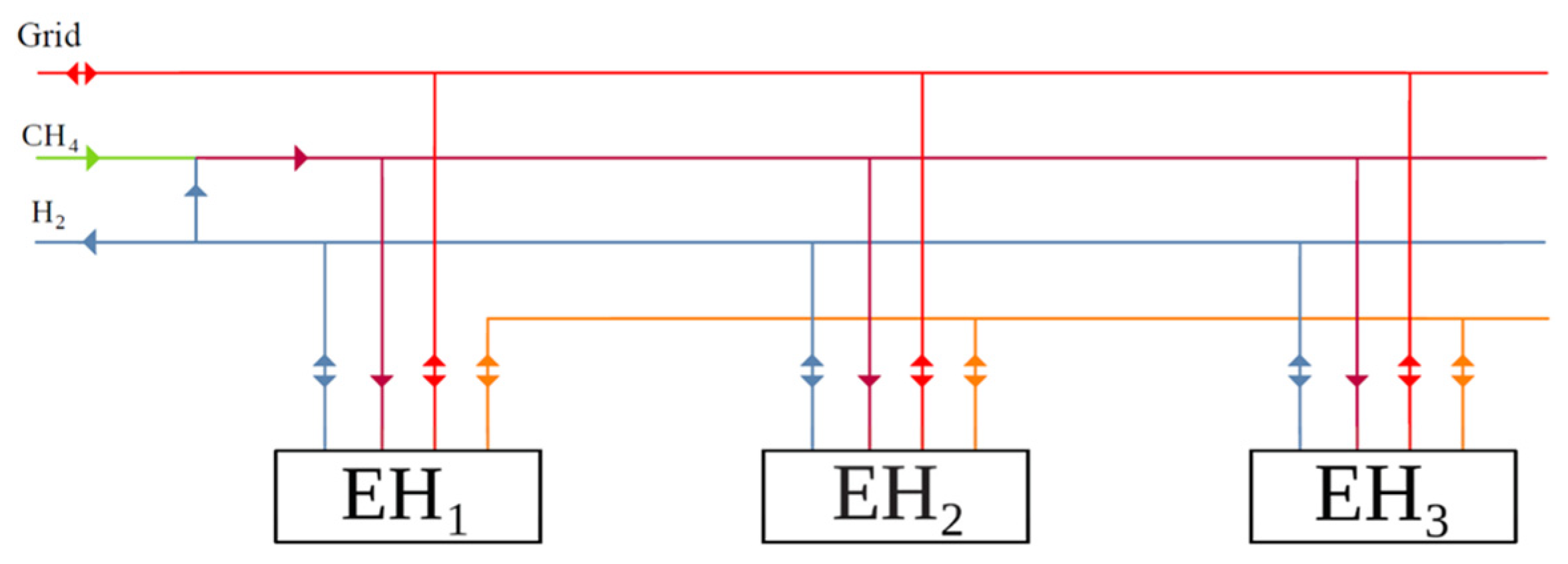
3.3. Self-Consumption-Based Representation
- To the electric vector (in red), which can both buy and sell electricity;
- To the thermal vector (in orange) with which the EHs can exchange heat;
- To the hydrogen vector (in blue), which can be exchanged between the EHs;
- To the gas network (in green), where natural gas is purchased—natural gas can be used in its pure form or mixed with hydrogen (mixture, in magenta) potentially up to 20% to serve the EHs.
- The first model focuses on the single EH;
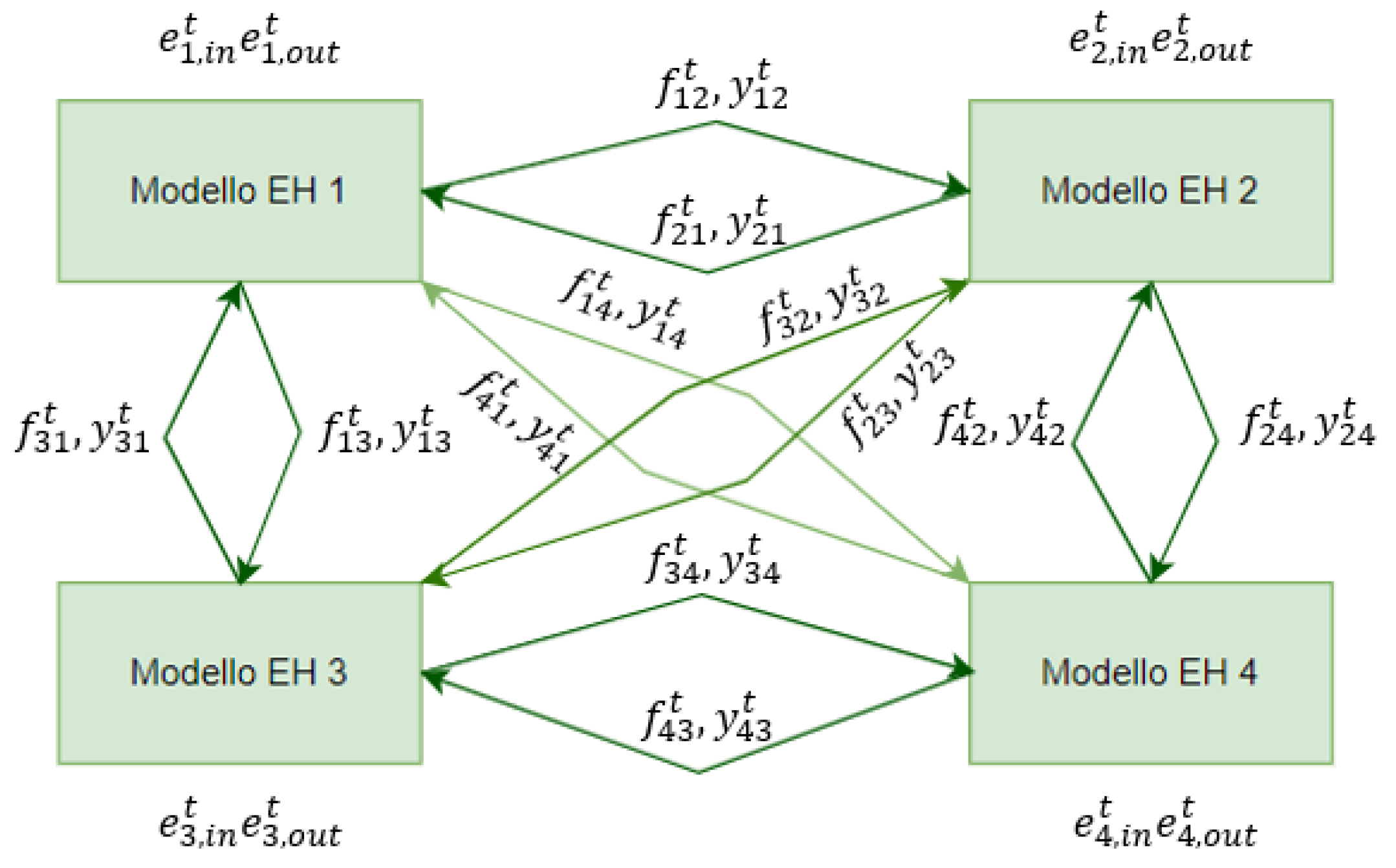
- The second model describes the multi-vector system, which is represented as a set of EHs, connected to each other through the three energy vectors.
- Limiting the values of the variables relating to generation and storage to a range between a minimum and a maximum value;
- Satisfying the balances of electricity, heat and gas in the network for each time period;
- Calculating the amount of energy stored in the storage systems for each instant (minimum storage at time t = 0);
- Determining the amounts of energy produced by each type of technology at any given moment;
- Limiting the operating region for the cogeneration plant;
- Making it so that the gas storage system cannot both supply and store gas at the same time (a few binary variables are introduced);
- Imposing (as binary variables):
- ○
- That the battery cannot supply and store electricity at the same time;
- ○
- That the heat storage system cannot supply and store heat at the same time;
- ○
- That the EH cannot sell and buy heat at the same time;
- ○
- That the EH cannot sell and buy gas at the same time.
- Flow balances of the electric vector;
- Flow balances of the heat vector;
- Flow balances of the gas vector;
- Limitation between 0 and max of energy flows between EHs of the three vectors;
- Weymouth Equation (12) to describe gas flows, linearized according to [34].
3.4. Joint Planning of Electricity and Hydrogen Transportation
- For hydrogen:
- ○
- Zonal hydrogen quantity balance constraints;
- ○
- Hydrogen production limits for the electrolyzers.
- For the electric system:
- ○
- Electric power balance for each bus;
- ○
- Limits for renewable power output;
- ○
- Power output and ramp rate for conventional generators;
- ○
- Branch flow for existing transmission lines (direct current approach);
- ○
- Flow-angle relations and flow limits for candidate lines.
3.5. Other Approaches
- DESA (Decentral Energy System Aggregation) derives costs for each decentral network area by performing distribution grid expansion planning for various supply tasks depending on the integration of technologies in the respective areas. The result of this model can then be used in central planning;
- In a fully linearized approach, CES regards the Central Energy System, taking data from DESA and the transmission grid into account;
- The result of the CES will then be given to the TEP (Transmission Expansion Planning) module, which focuses on a detailed expansion planning approach analyzing different expansion technologies and congestion management interventions;
- DESD (Decentral Energy System Disaggregation) undertakes the placing of renewable energy sources and other assets that have been centrally planned in CES for a Decentral Energy System (DES);
- The operation of a DES can be performed by the DESOP (Decentral Energy System Operational Planning) module and can be enriched by information from the CES;
- The DNEP (Distribution Network Expansion Planning) module implements an optimization approach to develop the distribution network expansion plan.
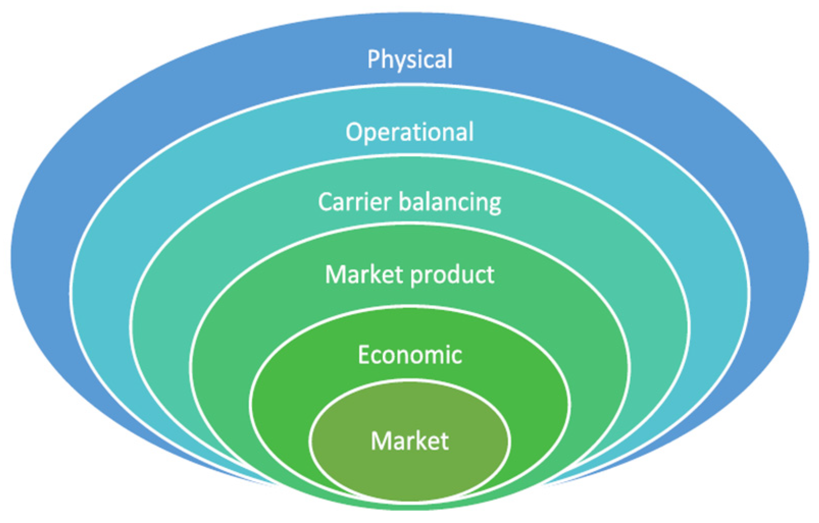
- Physical. Maximum flexibility within the energy vector, quantified by its operational range;
- Operational. Modulation capability for an energy carrier that an MES can provide with respect to (starting from) a given operating point. The operational flexibility of a device is divided into two components—upward and downward;
- Carrier-balancing. Operational flexibility for an energy carrier, reduced by the constraints imposed by the other energy carriers through conversion nodes. The energy vectors of MES are coupled and cannot be viewed independently. The operational flexibility available to an energy vector is also impacted by the constraints of other energy vectors;
- Market product. Carrier-balancing flexibility is subject to market product constraints, e.g., maximum allowed activation time and minimum service duration, which further limit the flexibility that can be provided by a cluster of resources;
- Economic. Flexibility that the MES operator can offer at a given cost for a specific service and accounting for MES economic objectives (to be optimized). A device will only participate in a given service if the revenues are greater than the cost of delivering that service;
- Market. Economic flexibility cleared and accepted by the market given the market requirements and other offers.
3.6. Computational Complexity, Convergence, Scalability and Robustness
- The computational complexity of an algorithm can be defined as the amount of resources required to run it. A particular focus should be placed on computation time (generally measured by the number of elementary operations required) and memory storage requirements;
- Convergence of an iterative algorithm occurs when, as the iterations proceed, the output gets closer and closer to some specific value. More precisely, no matter how small an error range you choose, if you continue long enough, the target function will eventually stay within that error range around the final value;
- The scalability of an algorithm regards its ability to handle increasing amounts of data or complexity without compromising its performance or efficiency;
- The robustness of an algorithm can be broadly defined as the change in the performance of a computational system in the face of changes in the nature of the environment in which that system operates, or in the task that the system is meant to perform. In other terms, it defines sensitivity to a change in the parameters defining the system to be simulated—if small changes in one parameter can create great changes in the calculated solution, this can be a symptom of the limited reliability of the results obtained in this way.
4. Conclusions
- Hybrid energy storage systems [66], which are diverse storage technologies coupled together in order to improve both transient speed and total amount of storable energy, so as to provide better services to the electric system;
- Digital twins [67], which are virtual modeling clones of entire network grids or parts of them, often coupled with Artificial Intelligence methodologies;
- The implementation of demand-side management [68] programs, which aim at providing flexibility to the electric system and parallel the effect that coupling with other carriers can provide;
- Industrial complexes, which are hard-to-abate industries [2] like steel mills where both electricity and other carriers (like hydrogen) can play a key role;
Funding
Conflicts of Interest
References
- European Commission. 2050 Long-Term Strategy. Striving to Become the World’s First Climate-Neutral Continent by 2050. Available online: https://climate.ec.europa.eu/eu-action/climate-strategies-targets/2050-long-term-strategy_en (accessed on 29 January 2025).
- Migliavacca, G.; Carlini, C.; Domenighini, P.; Zagano, C. Hydrogen: Prospects and Criticalities for Future Development and Analysis of Present EU and National Regulation. Energies 2024, 17, 4827. [Google Scholar] [CrossRef]
- Results of Pilot B. Report D5.2 of the SmartNet Project. 2019. Available online: https://smartnet-project.eu/wp-content/uploads/2019/05/D5.2.pdf (accessed on 29 January 2025).
- Project MAGNITUDE Web Site. Available online: https://www.magnitude-project.eu (accessed on 29 January 2025).
- Markensteijn, A.S. Mathematical Models for Simulation and Optimization of Multi-Carrier Energy Systems. Ph.D. Thesis, Delft University of Technology, Delft, The Netherlands, 2021. Available online: https://research.tudelft.nl/en/publications/mathematical-models-for-simulation-and-optimization-of-multi-carr (accessed on 6 February 2025).
- Mancarella, P. MES (multi-energy systems): An overview of concepts and evaluation models. Energy 2014, 65, 1–17. Available online: https://www.sciencedirect.com/science/article/abs/pii/S0360544213008931 (accessed on 27 February 2025).
- Shahidehpour, M.; Fu, Y. Tutorial: Benders Decomposition in Restructured Power Systems. Available online: http://motor.ece.iit.edu/ms/benders.pdf (accessed on 29 January 2025).
- European Commission Official Web Site. Available online: https://commission.europa.eu/index_en (accessed on 29 January 2025).
- Communication from the Commission to the European Parliament, the Council, the European Economic and Social Committee and the Committee of the Regions: Powering a Climate-Neutral Economy: An EU Strategy for Energy System Integration, 2020 COM (2020) 299 Final. Available online: https://eur-lex.europa.eu/legal-content/EN/TXT/PDF/?uri=CELEX:52020DC0299 (accessed on 29 January 2025).
- ACER. Electricity Infrastructure Development to Support a Competitive and Sustainable Energy System—2024 Monitoring Report. 2024. Available online: https://www.acer.europa.eu/monitoring/MMR/electricity_infrastructure_2024#:~:text=2024%20Monitoring%20Report,and%20competitive%20EU%20energy%20system (accessed on 29 January 2025).
- ACER. Official Web Site. Available online: https://www.acer.europa.eu/the-agency/about-acer (accessed on 29 January 2025).
- ENTSO-E. Official Web Site. Available online: https://www.entsoe.eu/ (accessed on 29 January 2025).
- ENTSO-G. Official Web Site. Available online: https://www.entsog.eu/ (accessed on 29 January 2025).
- ENTSO-E ENTSOG TYNDP Scenarios. Pathways to Carbon Neutrality in 2050. 2024. Available online: https://www.entsos-tyndp-scenarios.eu/ (accessed on 29 January 2025).
- Eiselt, H.A.; Sandblom, C.L. Operations Research; Springer Nature: Berlin/Heidelberg, Germany, 2022; Available online: https://link.springer.com/book/10.1007/978-3-030-97162-5?source=shoppingads&locale=en-it&gad_source=1&gclid=CjwKCAiA5pq-BhBuEiwAvkzVZWgiCUQdSosPFPw_u-Qq0ERV4PpFL1Rm35q6tlEcw6u7zet-g9NkxBoCG7EQAvD_BwE (accessed on 4 March 2025).
- Terlaky, T. Interior Point Methods of Mathematical Programming; Springer Nature: Berlin/Heidelberg, Germany, 1996; Available online: https://link.springer.com/book/10.1007/978-1-4613-3449-1 (accessed on 4 March 2025).
- Deliverable 1.2 of the FlexPlan Project. Probabilistic Optimization of T&D Systems Planning with High Grid Flexibility and Its Scalability. Available online: https://flexplan-project.eu/wp-content/uploads/2022/08/D1.2_20220801_V2.0.pdf (accessed on 29 January 2025).
- Wolsey, L.A. Integer Programming; Wiley: Hoboken, NJ, USA, 2020; Available online: https://www.wiley.com/en-us/Integer+Programming%2C+2nd+Edition-p-9781119606536 (accessed on 4 March 2025).
- Mancò, G.; Tesio, U.; Guelpa, E.; Verda, V. A review on MES modelling and optimization. Appl. Therm. Eng. 2024, 236, 121871. Available online: https://www.sciencedirect.com/science/article/pii/S1359431123019002 (accessed on 30 January 2025).
- Ntaimo, L. Computational Stochastic Programming; Springer Nature: Berlin/Heidelberg, Germany, 2024; Available online: https://link.springer.com/book/10.1007/978-3-031-52464-6?source=shoppingads&locale=en-it&gad_source=1&gclid=CjwKCAiA5pq-BhBuEiwAvkzVZZWzpqfKgMylS50_gPl--H9x_b0zaww_6zyoqLsj5EImbURbtoa2KRoCI0cQAvD_BwE (accessed on 4 March 2025).
- Ben-Tal, A.; El Ghaoui, L.; Nemirovski, A. Robust Optimization; Princeton Series in Applied Mathematics; Princeton University Press: Princeton, NJ, USA, 2009; Available online: https://www.amazon.it/Robust-Optimization-Aharon-Ben-Tal/dp/0691143684 (accessed on 4 March 2025).
- Official Site of the MATPOWER Library. Available online: https://matpower.org/ (accessed on 3 February 2025).
- Official Site of the MATLAB Programming Language. Available online: https://mathworks.com/products/matlab.html (accessed on 3 February 2025).
- PowerModels Library on the GitHub Repository. Available online: https://lanl-ansi.github.io/PowerModels.jl/stable/ (accessed on 3 February 2025).
- Official Site of the Julia Programming Language. Available online: https://julialang.org/ (accessed on 3 February 2025).
- Milano, F. Power flow analysis. In Chapter Part of the Book: Power System Modelling and Scripting of the Same Author; Springer Nature: Berlin/Heidelberg, Germany, 2010; Available online: https://link.springer.com/chapter/10.1007/978-3-642-13669-6_4 (accessed on 4 March 2025).
- Gan, L.; Low, S.H. Convex relaxations and linear approximation for optimal power flow in multiphase radial networks. In Proceedings of the 2014 Power Systems Computation Conference, Wroclaw, Poland, 18–22 August 2014; pp. 1–9. Available online: https://authors.library.caltech.edu/records/1fcqw-beg37 (accessed on 3 February 2025).
- Glover, J.D.; Sarma, M.S.; Overbye, T.J. Power System Analysis and Design, 5th ed.; Cengage Learning: Boston, MA, USA, 2012. [Google Scholar]
- Jacobian Matrix Definition in Microfluidics: Modelling, Mechanics and Mathematics. 2017. Available online: https://www.sciencedirect.com/topics/engineering/jacobian-matrix#definition (accessed on 4 March 2025).
- Johnen, M.; Pitzen, S.; Kamps, U.; Kateri, M.; Dechent, P.; Sauer, D.U. Modeling long-term capacity degradation of lithium-ion batteries. J. Energy Storage 2021, 34, 102011. Available online: https://www.sciencedirect.com/science/article/abs/pii/S2352152X20318466 (accessed on 3 February 2025).
- Wylie, E.B.; Streeter, V. Fluid Transients (Chapter 15); Mc. Graw Hill: New York, NY, USA, 1978. [Google Scholar]
- Migliavacca, G. Simulazione di Reti per il Trasporto di Fluido Comprimibile. Master’s Thesis, Politecnico di Milano, Milan, Italy, 1991. (In Italian; Available upon Request). [Google Scholar]
- Kollmann, W. Navier-Stokes Turbulence. In Theory and Analysis; Springer Nature: Berlin/Heidelberg, Germany, 2024; Available online: https://link.springer.com/book/10.1007/978-3-031-59578-3?source=shoppingads&locale=en-it&gad_source=1&gclid=CjwKCAiA5pq-BhBuEiwAvkzVZdKf5txHlQM7fvmvoRBzwt79DixQDehMuwJBnt0ZcN6DKgjOHpGekhoC9XcQAvD_BwE (accessed on 4 March 2025).
- Asghari, M.; Fathollahi-Fard, A.M.; Mirzapour Al-e-hashem, S.M.J.; Dulebenets, M.A. Transformation and Linearization Techniques in Optimization: A State-of-the-Art Survey. Mathematics 2022, 10, 283. [Google Scholar] [CrossRef]
- Yang, J.; Zhang, N.; Botterud, A.; Kang, C. Situation awareness of electricity-gas coupled systems with a multi-port equivalent gas network model. Appl. Energy 2020, 258, 114029. Available online: https://www.sciencedirect.com/science/article/abs/pii/S0306261919317167 (accessed on 18 March 2025).
- Dancker, J.; Wolter, M. A joined quasi-linear-state power flow calculation for integrated energy systems. IEEE Access 2022, 10, 33586–33601. [Google Scholar] [CrossRef]
- Courant, R.; Fredrichs, K.O.; Lewy, H. Uber die Differenzengleichungen der Mathematischen Physik. Math. Ann. 1928, 100, 32. Available online: https://gdz.sub.uni-goettingen.de/id/PPN235181684_0100 (accessed on 5 February 2025).
- Courant, R.; Friedrichs, K.; Lewy, H. Über die partiellen Differenzengleichungen der mathematischen Physik. Math. Ann. 1928, 100, 32–74. Available online: https://link.springer.com/article/10.1007/BF01448839 (accessed on 4 March 2025).
- Hafsi, Z.; Ekhtiari, A.; Ayed, L.; Elaoud, S. The linearization method for transient gas flows in pipeline systems revisited: Capabilities and limitations of the modelling approach. J. Nat. Gas Sci. Eng. 2022, 101, 104494. Available online: https://www.sciencedirect.com/science/article/abs/pii/S1875510022000853 (accessed on 6 February 2025).
- Demissie, A.; Zhu, W.; Taye Belachew, C. A multi-objective optimization model for gas pipeline operations. Comput. Chem. Eng. 2017, 100, 94–103. Available online: https://www.sciencedirect.com/science/article/abs/pii/S009813541730073X (accessed on 6 February 2025). [CrossRef]
- Gallagher, J.E. Isentropic Exponent Definition in Natural Gas Measurement Handbook; Elsevier: Amsterdam, The Netherlands, 2006; Available online: https://www.sciencedirect.com/topics/engineering/isentropic-exponent#:~:text=The%20isentropic%20exponent%20(%CE%BA)%20is,V%2Dcone%2C%20pitot) (accessed on 4 March 2025).
- Wolberg, J. Data Analysis Using the Method of Least Squares. In Extracting the Most Information from Experiments; Springer: Berlin/Heidelberg, Germany, 2006; Available online: https://link.springer.com/book/10.1007/3-540-31720-1 (accessed on 4 March 2025).
- Brown, A.; Foley, A.; Laverty, D.; McLoone, S.; Keatley, P. Heating and cooling networks: A comprehensive review of modelling approaches to map future directions. Energy 2022, 261, 125060. Available online: https://www.sciencedirect.com/science/article/pii/S0360544222019557 (accessed on 6 February 2025).
- Kuntuarova, S.; Licklederer, T.; Huynh, T.; Zinsmeister, D.; Hamacher, T.; Peri’c, V. Design and simulation of district heating networks: A review of modeling approaches and tools. Energy 2024, 305, 132189. Available online: https://www.sciencedirect.com/science/article/pii/S0360544224019637 (accessed on 6 February 2025).
- Migliavacca, G.; Rossi, M.; Siface, D.; Marzoli, M.; Ergun, H.; Rodriguez-Sanchez, R.; Hanot, M.; Leclercq, G.; Amaro, N.; Egorov, A.; et al. The Innovative FlexPlan Grid-Planning Methodology: How Storage and Flexible Resources Could Help in De-Bottlenecking the European System. Energies 2021, 14, 1194. Available online: https://www.mdpi.com/1996-1073/14/4/1194 (accessed on 7 February 2025). [CrossRef]
- Geidl, M. Integrated Modeling and Optimization of Multi-Carrier Energy Systems. Ph.D. Thesis, ETH Zurich, Zurich, Switzerland, 2007. No. 17141. Available online: https://www.research-collection.ethz.ch/handle/20.500.11850/123494 (accessed on 7 February 2025).
- Markensteijn, A.S.; Romate, J.E.; Vuik, C. A graph-based model framework for steady-state load flow problems of general multi-carrier energy systems. Appl. Energy 2020, 280, 115286. Available online: https://www.sciencedirect.com/science/article/pii/S0306261920307984 (accessed on 27 February 2025).
- Diestel, R. Graph Theory; Springer Nature: Berlin/Heidelberg, Germany, 2025; Available online: https://link.springer.com/book/10.1007/978-3-662-70107-2?source=shoppingads&locale=en-it&gad_source=1&gclid=CjwKCAiA5pq-BhBuEiwAvkzVZQi3LQ9C0B63G5KCCUtSWiBUJD5QM92GDIHP-G6pOwURxMjtagxHuhoCJtsQAvD_BwE (accessed on 4 March 2025).
- Simmini, F.; Cordieri, S.A. Modello Integrato del Sistema Energetico Locale; Report PORH2 D4.1.4.2. Milano, Italy 2024 (manuscript in preparation) (In Italian, available upon request).
- Wang, S.; Bo, R. Joint planning of electricity transmission and hydrogen transportation networks. IEEE Trans. Ind. 2022, 58, 2887–2897. Available online: https://ieeexplore.ieee.org/ielaam/28/9733857/9573477-aam.pdf (accessed on 11 February 2025).
- PlaMES. Project Web Site. Available online: https://plames.eu/ (accessed on 12 February 2025).
- PlaMES. Project Deliverable 2.2. Mathematical Formulation of the Model. 2020. Available online: https://plames.eu/wp-content/uploads/2020/11/20200630_Plames_D2.2_final.pdf (accessed on 12 February 2025).
- Corsetti, E.; Riaz, S.; Riello, M.; Mancarella, P. Modelling and deploying ME flexibility: The energy lattice framework. Adv. Appl. Energy 2021, 2, 100030. Available online: https://www.sciencedirect.com/science/article/pii/S2666792421000238 (accessed on 12 February 2025).
- Breeze, P. Combined Heat and Power; Elsevier: Amsterdam, The Netherlands, 2017; Available online: https://shop.elsevier.com/books/combined-heat-and-power/breeze/978-0-12-812908-1 (accessed on 4 March 2025).
- iDesignRES. Project Web Site. Available online: https://idesignres.eu/ (accessed on 13 February 2025).
- MOPO. Project Web Site. Available online: https://www.tools-for-energy-system-modelling.org/ (accessed on 13 February 2023).
- Sundar, K.; Misray, S.; Zlotniky, A.; Bent, R. Robust Gas Pipeline Network Expansion Planning to Support Power System Reliability. In Proceedings of the 2021 American Control Conference (ACC), New Orleans, LA, USA, 25–28 May 2021; Available online: https://ieeexplore.ieee.org/document/9483249 (accessed on 27 February 2025).
- Zhang, X.; Shahidehpour, M.; Alabdulwahab, A.S.; Abusorrah, A. Security-Constrained Co-Optimization Planning of Electricity and Natural Gas Transportation Infrastructures. IEEE Trans. Power Syst. 2015, 30, 2984–2993. Available online: https://ieeexplore.ieee.org/document/6987368 (accessed on 27 February 2025).
- Wald, G.; Sundar, K.; Sherwin, E.; Zlotnik, A.; Brandt, B. Optimal gas-electric energy system decarbonization planning. Adv. Appl. Energy 2022, 6, 100086. Available online: https://www.sciencedirect.com/science/article/pii/S266679242200004X (accessed on 27 February 2025).
- Birati, F.; Seifi, H.; Sepasian, M.S.; Nateghi, A.; Shafie-khah, M.; Catalao, J.P.S. Multi-Period Integrated Framework of Generation, Transmission, and Natural Gas Grid Expansion Planning for Large-Scale Systems. IEEE Trans. Power Syst. 2015, 30, 2527–2537. Available online: https://ieeexplore.ieee.org/document/6942215 (accessed on 27 February 2025).
- Thie, N.; Franken, M.; Schwaeppe, H.; Böttcher, L.; Müller, C.; Moser, A. Requirements for Integrated Planning of Multi-Energy Systems. In Proceedings of the 2020 6th IEEE International Energy Conference (ENERGYCON), Gammarth, Tunisia, 28 September–1 October 2020; Available online: https://ieeexplore.ieee.org/document/9236466 (accessed on 27 February 2025).
- Tangi, M.; Amaranto, A. Designing integrated and resilient multi-energy systems via multi-objective optimization and scenario analysis. Appl. Energy 2025, 382, 125281. Available online: https://www.sciencedirect.com/science/article/pii/S030626192500011X (accessed on 27 February 2025).
- Mostafa, M.; Vorwerk, D.; Heise, J.; Povel, A.; Sanina, N.; Babazadeh, D. Integrated Planning of Multi-energy Grids: Concepts and Challenges. In Proceedings of the NEIS 2022; Conference on Sustainable Energy Supply and Energy Storage Systems, Hamburg, Germany, 26–27 September 2022; Available online: https://ieeexplore.ieee.org/document/10048077 (accessed on 27 February 2025).
- Los Alamos National Laboratory’s Advanced Network Science Initiative. Available online: https://lanl-ansi.github.io/ (accessed on 13 February 2025).
- ANSI. Open Access Infrastructure Networks Simulation Libraries. Available online: https://lanl-ansi.github.io/software/ (accessed on 13 February 2025).
- Bocklisch, T. Hybrid energy storage systems for renewable energy applications. Energy Procedia 2015, 73, 103–111. Available online: https://www.sciencedirect.com/science/article/pii/S1876610215013508 (accessed on 25 February 2025). [CrossRef]
- Sifat, M.; Choudhury, S.M.; Das, S.K.; Ahamed, H.; Muyeen, S.M.; Hasan, M.; Ali, F.; Tasneem, Z.; Islam, M.; Islam, R.; et al. Towards electric digital twin grid: Technology and framework review. Energy AI 2023, 11, 100213. Available online: https://www.sciencedirect.com/science/article/pii/S2666546822000593 (accessed on 25 February 2025). [CrossRef]
- Gupta, P. Demand side management. In An Approach to Peak Load Smoothing; Scholar’s Press: London, UK, 2013; Available online: https://www.amazon.com/Demand-Side-Management-Approach-Smoothing/dp/3639511298 (accessed on 4 March 2025).
- Mishra, P.; Singh, G. Sustainable Smart Cities. In Enabling Technologies, Energy Trends and Potential Applications; Springer: Berlin/Heidelberg, Germany, 2023; Available online: https://link.springer.com/book/10.1007/978-3-031-33354-5 (accessed on 4 March 2025).
- Chowdhury, S.; Chowdhury, S.P.; Crossley, P.P. Microgrids and Active Distribution Networks; IET: London, UK, 2009; Available online: https://digital-library.theiet.org/doi/book/10.1049/pbrn006e (accessed on 4 March 2025).
- Rossini, M.; Rossi, M.; Siface, D. A surrogate model of distribution networks to support transmission network planning. In Proceedings of the 27th International Conference on Electricity Distribution, Rome, Italy, 12–15 June 2023; Available online: https://ieeexplore.ieee.org/document/10267731 (accessed on 18 March 2025).
- Mahmood, Z.; Puttini, R.; Erl, T. Cloud Computing: Concepts, Technology & Architecture; Pearson: London, UK, 2013. [Google Scholar]


| Unit | Gas | Electricity | Heat |
|---|---|---|---|
| Turbo compressor | control | consumed | |
| Heat pump | consumed | produced | |
| Gas boiler | consumed | produced | |
| Electric boiler | consumed | produced | |
| Circulation pump | consumed | control | |
| Gas turbine | consumed | produced | produced |
| Gas-fired generator | consumed | produced | |
| Power-to-gas | produced | consumed |
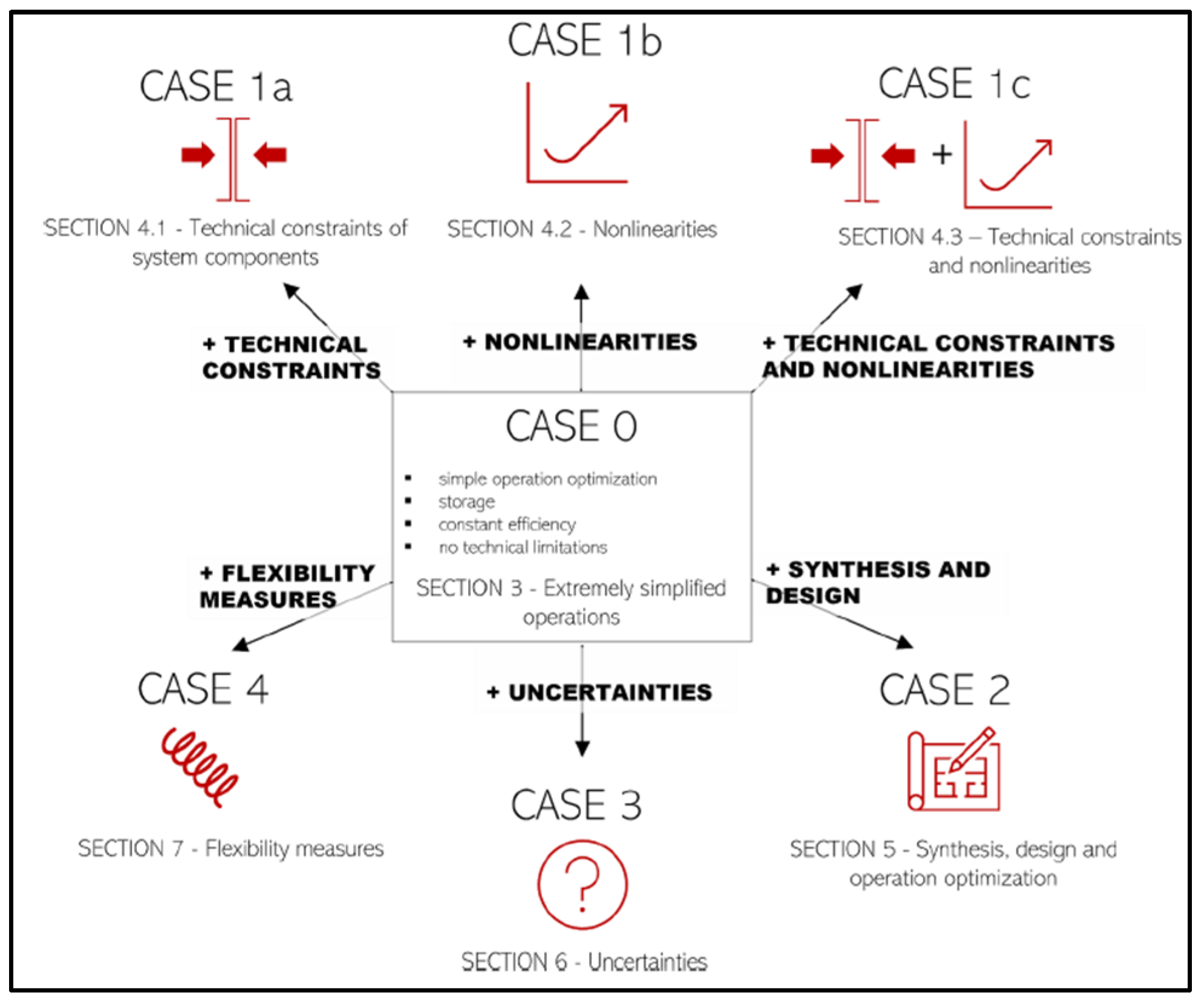
| Case | Description | Constraints | Mathematical Model |
|---|---|---|---|
| Case 0 | Optimal scheduling of MES (short term/daily operation horizon) |
| Linear optimization problem (LP)—no integer variables. The optimization can be carried out time step by time step (unless storage is included). |
| Case 1a | Same as case 0 with technical constraints of components |
| Binary decision variables must be included (e.g., to model technical minima or up and down time). Ramp rates couple different time steps. The problem is MILP optimization over the entire day. |
| Case 1b | Same as case 0 plus components non-linearities |
| Non-linear optimization. A possible alternative is the (piecewise) linearization of non-linear terms. |
| Case 1c | Case 0 plus both technical constraints and nonlinear terms | As case 1a + 1b | MILNP optimization. It becomes MILP if linearized. |
| Case 2 | Synthesis, design (e.g., system planning) and operation | As the previous ones | The correct timeframe is long-term (typically equal to the lifetime of the system). The model is MILNP or MILP. Decomposition techniques (e.g., Benders) are important. Sometimes, the operation optimization is decoupled from the synthesis problem (master–slave coupled problems). |
| Case 3 | Including uncertainty | As the previous ones | Two possible approaches: sensitivity analysis or optimization under uncertainty (by using either stochastic programming [20] or robust optimization [21]). |
| Case 4 | Including flexibility measures (i.e., the ability to guarantee the power balance through efficient operation changes: use of energy storage, energy substitution, inertia of thermal networks and buildings, demand response, etc.). | As the previous ones, plus extra equations modeling flexibility measures | Possible required modeling actions:
|
| Network | Node Type | Specified | Unknown |
|---|---|---|---|
| Gas | reference | p | W |
| load | W | p | |
| Electricity | slack | , δ | P, Q |
| generator (PV) | P | Q, δ | |
| load (PQ) | P, Q | , δ | |
| Heat | source reference slack | , p | , Δφ, W |
| load (source) | and Δφ < 0 | , p, W | |
| load (sink) | and Δφ > 0 | , p, W | |
| junction | W = 0 | , p |
| Computation Complexity | Scalability | Suitability of Different Models | |
|---|---|---|---|
| Load flow of MES | Solution of a separated system of equations for each simulation hour | This is the easiest model and the most scalable one (even more so if the resulting system is linear or at least convex). Variable normalization can help to treat “stiff” systems with numbers of very different orders of magnitude. | More complex models are possible, with compatibly with the size of the solving system, to allow for a more detailed representation of the system. |
| Dispatch optimization (e.g., market solutions) | Solution of an optimization problem. The hours are separately solved only if there is no integral constraint (e.g., storage systems). | If the solution of the subsequent time steps is decoupled, the problem, yet more complex than the load flow one, is still quite scalable and is fit for simulating real-size systems. | Static models are typically used. A linearization is also often required, especially when there is a maximum amount of time within which the solution must be calculated (e.g., one market solution to be obtained every 15 min or every hour). |
| Planning of MES | Solution of one very large optimization problem, including both dispatch and investment variables. Investment variables are typically integer ones, resulting in a MILP model. | This is the most complex problem; the one with biggest dimensionality, which is additionally typically formulated as a MILP. Decoupling techniques (e.g., Benders’) as well as parallel computing can help to manage this while preserving reasonable scalability. The timestep dimension should compromise between preserving scalability and correctly representing intertemporal constraints of the storage systems. | Linear (or linearized) models are needed, and every type of complexity must be evaluated against numerical complexity. |
Disclaimer/Publisher’s Note: The statements, opinions and data contained in all publications are solely those of the individual author(s) and contributor(s) and not of MDPI and/or the editor(s). MDPI and/or the editor(s) disclaim responsibility for any injury to people or property resulting from any ideas, methods, instructions or products referred to in the content. |
© 2025 by the author. Licensee MDPI, Basel, Switzerland. This article is an open access article distributed under the terms and conditions of the Creative Commons Attribution (CC BY) license (https://creativecommons.org/licenses/by/4.0/).
Share and Cite
Migliavacca, G. Multi-Energy Static Modeling Approaches: A Critical Overview. Energies 2025, 18, 1826. https://doi.org/10.3390/en18071826
Migliavacca G. Multi-Energy Static Modeling Approaches: A Critical Overview. Energies. 2025; 18(7):1826. https://doi.org/10.3390/en18071826
Chicago/Turabian StyleMigliavacca, Gianluigi. 2025. "Multi-Energy Static Modeling Approaches: A Critical Overview" Energies 18, no. 7: 1826. https://doi.org/10.3390/en18071826
APA StyleMigliavacca, G. (2025). Multi-Energy Static Modeling Approaches: A Critical Overview. Energies, 18(7), 1826. https://doi.org/10.3390/en18071826